University of Pretoria Department of Economics Working Paper Series

Bank-Lending Channel in South Africa: Bank-Level Dynamic Panel Date Analysis Moses M. Sichei University of Pretoria Working Paper: 2005-10 November 2005 __________________________________________________________ Department of Economics University of Pretoria 0002, Pretoria South Africa Tel: +27 12 420 2413 Fax: +27 12 362 5207 http://www.up.ac.za/up/web/en/academic/economics/index.html

Bank-Lending Channel in South Africa: Bank-Level Dynamic

Panel Data Analysis

Moses Muse Sichei

Department of Economics, University of Pretoria, 0002 Pretoria, South Africa

Email: sichei@yahoo.co.uk or moses.sichei@up.ac.za

November 21, 2005

__________________________________________________________

Abstract

The paper investigates the bank-lending channel (BLC) of monetary policy in South Africa

using quarterly bank-level data for the period 2000Q1-2004Q4. Capital adequacy and bank size

are used as indicators for information problems faced by banks when they look for external

finance. Utilising dynamic panel estimation methods the study shows that BLC operates in South

Africa. The finding has some policy implications. First, there is need to coordinate monetary

policy with financial innovations and prudential banking regulations. Second, the overall effects

of monetary policy pursued by the South African Reserve Bank cannot be completely

characterised by interest rates only.

JEL classification : E5 ;E52 ; G21 Keywords : Monetary policy transmission ; Bank-lending channel ; Dynamic panel ; GMM

estimator

2

1.Introduction

Monetary policy transmission mechanisms are the channels through which changes in

monetary policy instruments generate the desired policy goals such as economic growth

and price stability1. Schmidt-Hebbel (2003) highlight some difficulties faced in

attempting to identify the transmission channels for monetary policy in emerging

economies like South Africa. First, emerging economies are subject to greater volatility

and monetary policy regime changes. Second, there is a dearth of empirical studies on

emerging countries due to lack of data. Finally, much of economic theory is conceived

for industrial countries.

The Journal of Economic Perspectives fall 1995 edition contains papers presented in a

symposium on monetary transmission mechanisms (Mishkin 1995, Bernanke and Gertler,

1995, and Taylor, 1995). Mishkin (1995) identifies four channels of monetary policy

transmission; interest rate channel, credit channel (balance-sheet and bank-lending

channel), the exchange rate channel and other asset prices channel. The study focuses on

the bank-lending channel (BLC).

Kashyap and Stein (1993) argues that under the lending view of monetary

transmission, there are three assets; money, publicly issued bonds and intermediated

loans. Under this view, the banks play two roles. They create money and make loans

(maturity transformation), which unlike buying bonds the household sector cannot

1 The other objectives are full-employment, international competitiveness and financial stability.

3

perform. Specifically, banks are suited to handle certain types of borrowers with high

asymmetric information problems e.g. small firms.

In the three-asset world, monetary policy can affect investment not only through its

effect on interest rates but also via its impact on the supply of bank loans. Some banks

may, however, insulate their loan portfolio from the tight monetary policy by resorting to

non-traditional sources of finance. Thus the decrease in bank loans is likely to differ

among banks.

There is abundant evidence on the empirical relationship between monetary policy,

bank loans and economic activity (Kashyap and Stein, 2000, Kishan and Opiela, 2000,

Huang, 2003, Sevestre, Savignac and Loupias, 2002). The general conclusion in most of

the studies is that tight monetary policy leads to a drop in bank credit, which has large

negative impact on economic activity.

The study employs dynamic panel data approach to test how bank characteristics

(capital adequacy and bank assets) in South Africa affect the response of loan supply

after a change in monetary policy. The principal finding is that the BLC operates in

South Africa.

The rest of the paper is organised as follows. Section 2 briefly reviews monetary

policy in South Africa. Section 3 specifies the model. Section 4 deals with estimation

4

issues while Section 5 reports the results. The main insights and policy recommendations

are presented in Section 6.

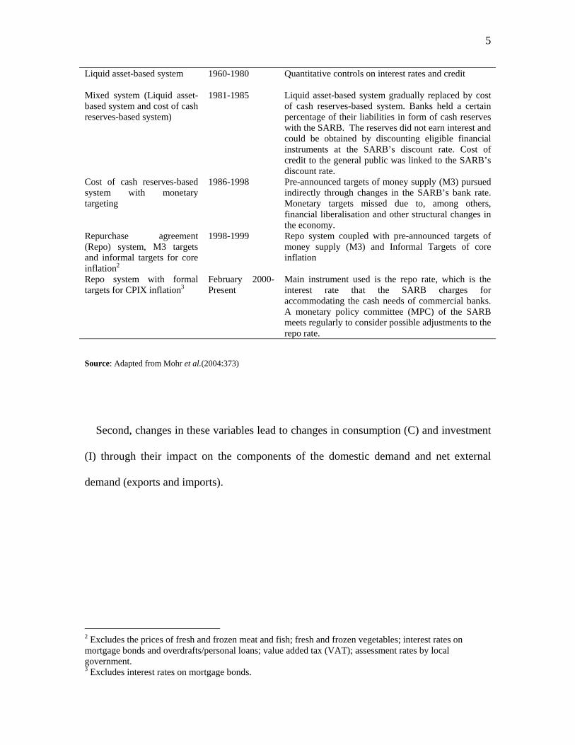
2. Monetary policy in South Africa

According to Mohr et al. (2004:373), monetary policy in South Africa can be divided

into five regimes; Liquid-asset based system, mixed system, cost of cash reserves based

system with monetary targeting, repurchase agreement (repo) system with monetary

targeting and informal inflation targeting, and repo system with formal inflation

targeting. These regimes are presented in Table 1. The focus of the study is on the last

regime, which uses the repo rate and formal inflation targets.

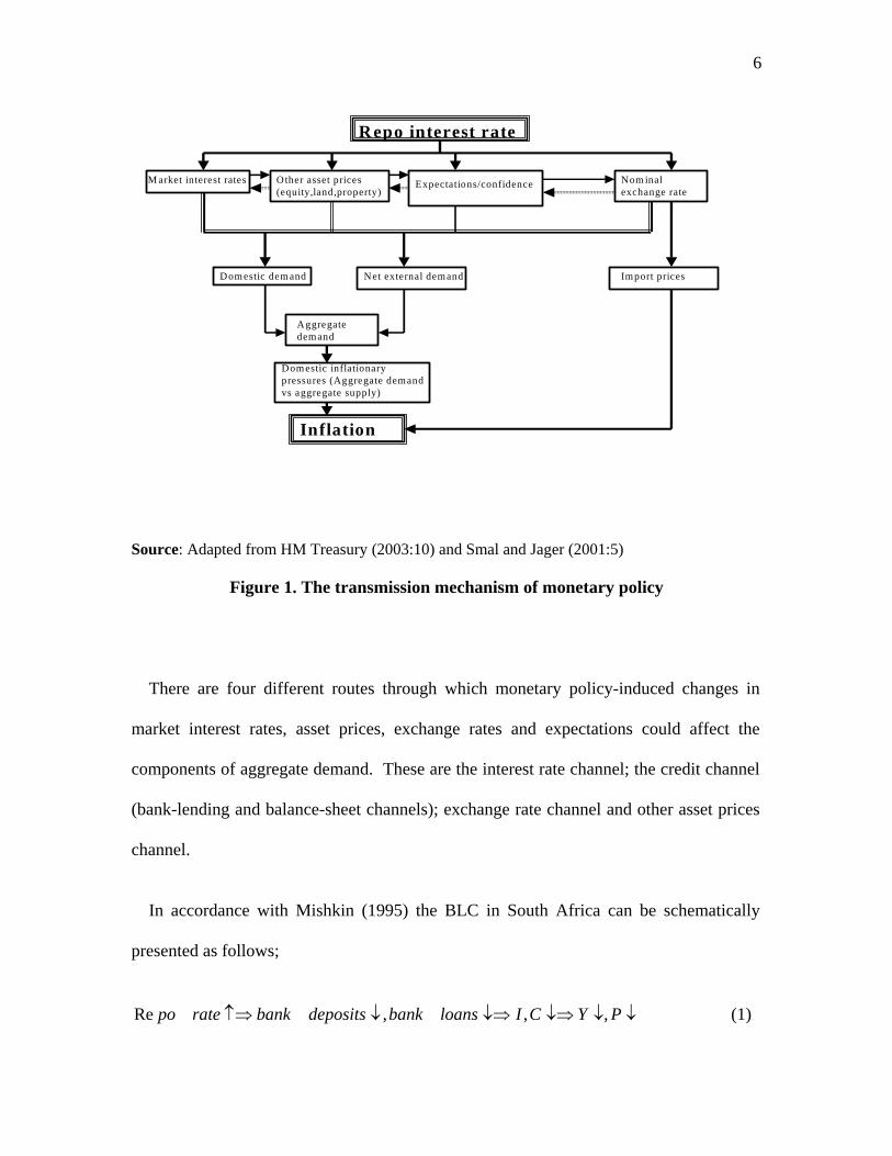
Figure 1 is a diagrammatic representation of the channels that are likely to be involved

in the monetary transmission mechanism in South Africa. Using the current monetary

policy regime (last row in Table 1), there are a number of steps in the monetary policy

transmission process.

First, a change in the repurchase agreement rate (repo) by the South African Reserve

Bank (SARB) affects the market interest rates (rates for deposits and lending), asset

prices, expectations and nominal exchange rates.

Table 1 Monetary policy regimes in South Africa Policy regime Period Features

5

Liquid asset-based system 1960-1980 Quantitative controls on interest rates and credit

Mixed system (Liquid asset-based system and cost of cash reserves-based system)

1981-1985 Liquid asset-based system gradually replaced by cost of cash reserves-based system. Banks held a certain percentage of their liabilities in form of cash reserves with the SARB. The reserves did not earn interest and could be obtained by discounting eligible financial instruments at the SARB’s discount rate. Cost of credit to the general public was linked to the SARB’s discount rate.

Cost of cash reserves-based system with monetary targeting

1986-1998 Pre-announced targets of money supply (M3) pursued indirectly through changes in the SARB’s bank rate. Monetary targets missed due to, among others, financial liberalisation and other structural changes in the economy.

Repurchase agreement (Repo) system, M3 targets and informal targets for core inflation2

1998-1999 Repo system coupled with pre-announced targets of money supply (M3) and Informal Targets of core inflation

Repo system with formal targets for CPIX inflation3

February 2000-Present

Main instrument used is the repo rate, which is the interest rate that the SARB charges for accommodating the cash needs of commercial banks. A monetary policy committee (MPC) of the SARB meets regularly to consider possible adjustments to the repo rate.

Source: Adapted from Mohr et al.(2004:373)

Second, changes in these variables lead to changes in consumption (C) and investment

(I) through their impact on the components of the domestic demand and net external

demand (exports and imports).

2 Excludes the prices of fresh and frozen meat and fish; fresh and frozen vegetables; interest rates on mortgage bonds and overdrafts/personal loans; value added tax (VAT); assessment rates by local government. 3 Excludes interest rates on mortgage bonds.

6

Repo interest rate

M arket interest rates Nom inal exchange rate

Expectations/confidenceOther asset prices (equity,land,property)

Dom estic dem and Net external demand

Aggregate demand

Dom estic inflationary pressures (Aggregate demand vs aggregate supply)

Inflation

Import prices

Source: Adapted from HM Treasury (2003:10) and Smal and Jager (2001:5)

Figure 1. The transmission mechanism of monetary policy

There are four different routes through which monetary policy-induced changes in

market interest rates, asset prices, exchange rates and expectations could affect the

components of aggregate demand. These are the interest rate channel; the credit channel

(bank-lending and balance-sheet channels); exchange rate channel and other asset prices

channel.

In accordance with Mishkin (1995) the BLC in South Africa can be schematically

presented as follows;

↓↓↓⇒↓⇒↓↑⇒ PYCIloansbankdepositsbankratepo ,,,Re (1)

7

Equation 1 states that an increase in the repo rate by the SARB curbs bank deposits

and demand for loans to finance investment and consumption. Depending on the

elasticity of aggregate supply and demand, national income or prices may fall.

One implication of the BLC is that monetary policy has greater effects on small banks,

which cannot cushion themselves against tight monetary policy. It also underscores the

fact that if prudential regulations allow banks greater ability to raise non-reservable funds

(e.g.CD), the potency of monetary policy is impaired.

The focus of this paper is on the BLC. However, there are some points that should be

emphasized. First, as pointed out by Mohr et al. (2004: 523), the link between the

interest rate and investment spending is quite crucial for the BLC. Second, the

transmission mechanisms works through various channels and it is not easy to isolate one

of them. Third, the outcome of the process is quite uncertain in most cases. Finally,

there is always a time lag between the policy action and its eventual impact on the real

output (Y) and price level (P).

3. Model specification

The study uses an empirical specification based on Kashyap and Stein (1993);

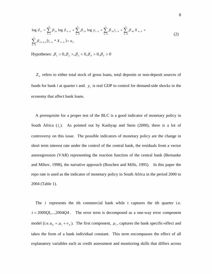
8

( ) itkitktk

ik

kkitk

kktk

kktk

kkitkit

uXi

XiyZZ

+

++++=

−−=

+

=−

=−

=−

=−

∑

∑∑∑∑

*

logloglog

1

0)5(

1

04

1

03

1

02

2

11

β

ββββ (2)

Hypotheses: 0,0,0,,0 54321 >><>> βββββ

refers to either total stock of gross loans, total deposits or non-deposit sources of

funds for bank i at quarter t and. is real GDP to control for demand-side shocks in the

economy that affect bank loans.

itZ

ty

A prerequisite for a proper test of the BLC is a good indicator of monetary policy in

South Africa ( ). As pointed out by Kashyap and Stein (2000), there is a lot of

controversy on this issue. The possible indicators of monetary policy are the change in

short term interest rate under the control of the central bank, the residuals from a vector

autoregression (VAR) representing the reaction function of the central bank (Bernanke

and Mihov, 1998), the narrative approach (Boschen and Mills, 1995). In this paper the

repo rate is used as the indicator of monetary policy in South Africa in the period 2000 to

2004 (Table 1).

ti

The represents the ith commercial bank while t captures the tth quarter i.e.

. The error term is decomposed as a one-way error component

model (i.e.

i

42004,...,12000 QQt =

itiitu νµ += ). The first component, iµ , captures the bank specific-effect and

takes the form of a bank individual constant. This term encompasses the effect of all

explanatory variables such as credit assessment and monitoring skills that differs across

9

banks but remains constant over time. itν is an idiosyncratic remainder error term

assumed to be white noise. Centred quarterly dummy variables for quarters 1 to 3 are

also included. These dummy variables take values of 0.75 and –0.25 otherwise.

A bank’s loan supply reaction to monetary policy is assumed to depend linearly on the

bank’s balance sheet strength (bank characteristics i.e. ), which can be proxied by

bank size ( ) and capitalisation ( ). Bank size and capitalisation are measures of

bank’s health that affect the external finance premium. These measures are defined as

follows;

itX

itS itK

∑=

−=24

1log1log

iititit A

NAS (3)

∑ ∑= =

⎟⎟⎠

⎞⎜⎜⎝

⎛−=

20

1

24

1

11t i it

it

it

itit A

CNTA

CK (4)

Where and are total assets and capital, respectively. Equations 3 and 4 show

the normalisation of the bank characteristics with respect to their average across all the

banks with a view to computing indicators that sum to zero over all observations. The

average of the interaction term is therefore zero and hence the parameters

itA itC

itt Xi * )5( k+β

in Equation 2 are interpretable as the overall monetary policy effect on the variable being

explained (loans, deposits or non-deposit funding related liabilities).

A dynamic panel data model is used for two reasons. First, there is a close banker-

customer relationship that develops and may create lock-in effects thus making it costly

10

for the borrower to change a bank (Rajan, 1992). Thus lagged loans affect current loans.

Second, monetary policy only impacts lending behaviour with a lag due to contractual

commitments (e.g. floating and fixed charges on movable and immovable assets,

respectively). Hence, lagged values of the explanatory variables also affect current loans

with a lag.

4. Estimation framework

The dynamic nature of the model in Equation 2 facilitates a better understanding of the

dynamics of loan adjustment. However, as pointed out by Baltagi (2001), the dynamic

panel data regression in Equation 2 is characterised by two sources of persistence over

time; autocorrelation due to the presence of a lagged dependent variable among the

regressors and bank-specific effects characterising the heterogeneity among the

commercial banks.

The inclusion of the lagged dependent variable renders the OLS estimator biased and

inconsistent even if the remainder error term ( itν ) is not serially correlated. Nickell

(1981) shows that the within estimator will be biased of order ( )1−TO and its consistency

depends on T being large. One prominent way to address the problem faced in dynamic

panel data has been through the first-differenced generalised method of moments (GMM)

estimator as suggested by Arrellano and Bond (1991).

Blundell and Bond (1998) and Kruiniger (2000) highlight some pitfalls of first

differenced GMM (Arrellano and Bond, 1991) estimator when using persistent data or

11

close to random walk. The main problem is that the instruments used in the standard

first-differenced GMM estimator become less informative in two cases. First, as 1β in

Equation 2 increases to unity, and second as the relative variance of the fixed effects

increases i.e. ∞→⎟⎟⎠

⎞⎜⎜⎝

⎛2

2

ν

µ

σσ

. Where and . )(2iVar µσ µ = )(2

itVar νσν =

Arrellano and Bover (1995) and Blundell and Bond (1998) demonstrate that when

11 =β the instruments used in first differenced GMM estimators are no longer correlated

with the first differences of the regressors. Additionally, some moment conditions

become discontinuous at 11 =β (Kruiniger, 2000).

The alternative approach is the Arrellano and Bover (1995) systems estimator, which

exploits an assumption about the initial conditions processes to obtain additional linear

moment conditions that remain informative even for persistent series4. This method

transforms the data using orthogonal forward deviation (Equation 25 in Arrellano and

Bover, 1995). This transformation subtracts the mean of the remaining future

observations available in the sample from each of the forward (T-1) observations.

This transformation has a number of important characteristics. First, it eliminates

bank-specific effects and keeps the orthogonality among the transformed errors. Second,

since the rows of the transformation matrix add up to zero, the permanent effects are

eliminated. Finally, the transformation matrix is upper triangular so that lags of

4 Most variables in this study are persistent (Table 6 in the appendix).

12

predetermined variables are valid instruments in the transformed equations. Blundell and

Bond (1998) demonstrate that the systems estimator results in substantial efficiency gains

and reduced bias, particularly with persistent data.

5. Estimation results

The study uses a sample of 24 banks out of 38 in existences as at December 2004.

The selection of the estimation period (2000Q1 to 2004Q4) is predicated on the need to

test BLC within one single monetary policy regime in South Africa (repo system and

inflation targeting in Table 1). Capitalisation adequacy and bank size are used to

discriminate banks according to their external finance costs.

There are two conditions for the BLC to work in South Africa. First, there should be

bank-dependent customers in South Africa. Second, monetary policy by the SARB

should be able to affect the supply of loans so that the decrease in loan supply depresses

real aggregate spending in South Africa. The first condition generally holds in South

Africa in the formal economy. Therefore the focus is on testing the second condition.

The study begins by first testing the prerequisite conditions for the SARB to be able to

affect loan supply.

5.1 The effect of monetary policy on deposit mobilisation

The first question that needs to be answered is do banks in South Africa experience a

fall in deposits following a monetary contraction? Columns 3 and 6 of Table 2 present

13

the results for the effect of monetary policy on bank deposits using capital adequacy and

bank size to discriminate banks. The Sargan over-identifying restriction confirms the

validity of lagged levels dated t-3 to t-5 as instruments.

First, the results show that an increase in the repo rate significantly reduces bank

deposits in South Africa (Equation 1). Thus tight monetary policy is inimical to the

deposit mobilisation function of commercial banks in South Africa.

Second, bank deposits increase by 1.8 per cent following 1 per cent increase in real

GDP. This is consistent with expectation since a booming economy would tend to have

many economic agents with excess savings, which commercial banks can mobilise.

Third, the effect of bank characteristics on deposits differs. On one hand an increase in

bank capital-asset ratio beyond the banking industry-wide average (Equation 4) leads to a

reduction in deposits. This finding is expected given the fact that banks with high capital

asset-ratio have less deposits (Tables 4 and 5 in the appendix). On the other hand an

increase in bank size (Equation 3) leads to an increase in deposits. This is a confirmation

of the fact that large banks have large deposits (Tables 4 and 5).

Finally, the joint effects of the repo rate and bank characteristics (capital-asset ratio

and bank size) are insignificant implying that the level of deposits falls uniformly

regardless of differences in balance sheet strength (information asymmetry). Thus, in

14

general deposits tend to fall following tight monetary policy, which satisfies one of the

conditions of BLC.

5.2 The effect of monetary policy on non-deposit sources of finance

The second question is can banks in South Africa replace the tight monetary policy-

induced lose in deposits by other sources of funds? To answer this question the non-

deposit funding related liabilities from the private sector is used to proxy other sources of

funds. Columns 4 and 7 of Table 2 present the results that attempt to answer this

question. The Sargan over-identifying restriction confirms the validity of lagged levels

dated t-3 to t-5 as instruments.

First, using capitalisation, an increase in the repo rate has a significant negative effect

on non-deposit funding related liabilities. However, using bank size the repo rate has no

effect on non-deposit funding related liabilities.

Second, an increase in real GDP leads to a reduction in non-deposit funding related

liabilities. This can be rationalised by the fact that robust economic activity is associated

with high deposits implying reduced need to seek other sources of finance.

Third, banks, which are highly capitalised, seek less non-deposit funding related

liabilities from the private sector. However, large banks tend to seek more non-deposit

funding related liabilities.

Table 2 Orthogonal forward deviation transformation GMM estimation results

Capital adequacy Bank size

Loans Deposits Other funding liabilities

Loans Deposits Other funding liabilities

Loans (-1) 0.934*** (27.699)

0.811***(23.350)

Deposits(-1)

0.398***(16.273)

0.449***(98.162)

Other funding liabilities (-1)

0.245*** (8.951)

0.245***(11.091)

Repo rate -0.018*** (-2.653)

-0.020*** (-3.749)

-0.285*** (-2.807)

-0.027*** (-3.739)

-0.015*** (-6.247)

0.101 (1.104)

Real GDP -0.512*** (-7.062)

1.833*** (9.193)

-31.163*** (-14.714)

-0.393** (-2.313)

1.803*** (16.302)

-30.006 *** (-21.746) Real capital -6.086***

(-3.380) -4.668*** (-3.902)

-43.039*** (-4.029)

Real capital*repo rate 0.682*** (3.531)

-0.007 (-0.088)

0.243 (0.207)

Bank size 0.389*** (4.448)

0.509*** (10.164)

3.725** (3.842)

Bank size*repo rate 0.021** (2.591)

-0.003 (-0.549)

-0.159*** (-3.293)

Quarter 1 dummy 0.158*** (10.580)

-2.349*** (-11.823)

0.139***(18.202)

-2.634*** (-18.606)

Quarter 2 dummy 0.073*** (5.706)

0.142 (0.586)

0.071***(8.918)

-0.010 (-0.119)

Quarter 3 dummy 0.024** (2.366)

-1.000*** (-16.235)

0.015***(2.902)

-1.006*** (-13.187) Diagnostic statistics

Adjusted R-squared 0.549 0.415 0.048 0.58 0.615 0.118Instrument rank 25.000 24.000 24.000 24.000 24.000 24.000Sargan J statistic 23.472(0.217) 19.886(0.225) 16.821(0.397) 21.789(0.295) 20.920(0.182) 18.621(0.289)

Notes: (i) *, ** and *** are 10%, 5% and 1% significance levels, respectively. (ii) Instrumentation: Lagged dependent variable dated 3−t to 5−t

Finally, the joint effects of contractionary monetary policy and bank characteristics

differ. On one hand capital-asset ratio is insignificant implying that the level of non-

deposits funding related liabilities falls uniformly regardless of differences in capital

(information asymmetry). On the other hand contractionary monetary policy leads to

increased levels of non-deposit funding related liabilities. Thus the reserve bank is

unable to effectively control the non-deposit funding related liabilities from the public.

5.3 The effect of monetary policy on bank loans

Having confirmed the conditions for BLC, the actual test is performed in the columns

2 and 5 of Table 2. BLC exists if the coefficients associated with the joint effects of the

repo rate and bank characteristics are positive. A non-significant coefficient may indicate

either absence of BLC or that the chosen bank characteristic does not appropriately

discriminate banks in South Africa according to their external finance cost.

First, the coefficient for the repo is significantly negative, which is consistent with the

interest rate channel and shows that bank loan supply falls as monetary policy tightens

and vice versa.

Second, there is a negative relationship between real GDP and bank loans. This is

inconsistent with expectation implying that banks tend to lean against the tide. Thus

recessions are characterised by banks trying to lend so as to prop up businesses and vice

versa.

17

Third, the partial effect of bank characteristics is ambiguous. Capital-asset ratio has a

significant negative effect on bank loans while bank size has a significant positive effect.

This is not surprising given the descriptive statistics in Tables 4 and 5 in the appendix

where it is apparent that small banks tend to have high capital-asset ratio.

Fourth, the joint effect of monetary policy and bank characteristics is significantly

positive implying that banks with strong balance sheets in terms of capital-asset ratio and

total assets can cushion the effects of tight monetary policy on their loan portfolio. This

effectively confirms the presence of BLC in South Africa. This finding is consistent

results from the US (e.g. Kashyap and Stein, 2000, Kishan and Opiela, 2000), who find

that size and capitalisation have significant impact on bank lending.

6. Conclusions

The aim of the paper was to check the existence of BLC in South Africa over the

period 2000Q1 to 2004Q4. This period was selected on account of same monetary

policy regime (i.e. inflation targeting and repo system). The study employs capital

adequacy and bank size to discriminate banks. The Arrellano and Bover (1995)

estimation framework is used since it is robust to persistent data.

Using both bank size and capital-asset ratio the study finds that BLC operates in South

Africa. The finding of BLC has a number of implications (Kashyap and Stein (1993).

18

First, monetary policy has distributional consequences in the banking sector.

Specifically, the cost of tight monetary policy might fall more on small banks and their

customers. These distributional considerations may be important when formulating

monetary policy in South Africa.

Second, the fact that large banks in South Africa can cushion the effects of tight

monetary policy on their loan portfolio implies that financial innovations and prudential

bank regulations can affect the potency of monetary policy. Thus there is need to co-

ordinate of prudential bank regulation, financial innovations and monetary policy.

Increase in the size of banks in South Africa may drive a wedge between monetary

policy conducted by SARB and the banking system. This policy recommendation has

implication for the deal between ABSA Bank and Barclays bank (Table A.1)5. The

resultant banking conglomerate may use its huge capital base to cushion the effects of

tight monetary policy.

Finally, using the repo rate as a measure of cost of financing may give a misleading

picture of the extent to which investment in different sectors is influenced by monetary

policy.

5 Barclays bank Plc is to invest 33 billion rands in Absa bank.

19

References

Arrellano, M. & Bond, S. (1991). Some tests of specification for panel data: Monte Carlo

evidence and an application to employment equations. Review of Economic Studies,

58, 277-297.

Arrellano, M. & Bover, O. (1995). Another look at the instrumental variable estimation

of error-components models. Journal of Econometrics, 68, 29-51.

Baltgagi, B.H. (2001), Econometric analysis of panel data. Second edition. New York:

John Wiley.

Bernanke, B.S. & Blinder, A. (1988). Credit, money and aggregate demand. American

Economic Review, 82, 901-21.

Bernanke, B.S. & Gertler, M. (1995). Inside the black box: The credit channel of

monetary policy. Journal of Economic Perspectives, 9(4), 27-48.

Bernanke, B.S. & Mihov, I. (1998). Measuring monetary policy. Quarterly Journal of

Economics, 113(3), 869-902.

Blundell, R. & Bond, S. (1998). Initial conditions and moment restrictions in dynamic

panel data models. Journal of Econometrics, 87, 115-143.

Boschen, J. & Mills, J. (1995). The effects of counter-cyclical policy on money and

interest rates: An evaluation of evidence from FOMC. Working Paper No. 91-20,

Federal Reserve Bank of Philadelphia.

Hadri, K. (2000). Testing for stationarity in heterogeneous panel data. Econometric

Journal, 3(2), 148-161.

Huang, Z. (2003). Evidence of a bank lending channel in the UK. Journal of Banking &

20

Finance, 27, 491-510.

Im, K.S., Pesaran, M.H. & Shin, Y. (2003). Testing for unit roots in heterogeneous

panels.

Journal of Econometrics, 115, 53-74.

Kashyap, A.K. & Stein, J.C. (1993). Monetary policy and bank lending. NBER Working

Paper series number 4317.

Kashyap, A.K. & Stein, J.C. (2000). What do a million observations on banks say about

the transmission of monetary policy? American Economic Review, 90, 407-428.

HM Treasury. (2003). The EMU and the monetary transmission mechanism. Retrieved

June 4, 2005, from http://news.bbc.co.uk/1/shared/spl/hi/europe/03/euro/pdf/5.pdf

Kishan, R. P. & Opiela, R. P. (2000). Bank size, bank capital, and the bank lending

channel. Journal of Money, Credit and Banking, 32, 121-141.

Kruiniger, H. (2000). GMM estimation of dynamic panel data models with persistent

data. Working Paper No.428, Department of Economics, University of London.

Levin, A., Lin.C.F. & Chu,C. (2002). Unit root tests in panel data: Asymptotic and finite

sample properties. Journal of Econometrics, 108, 1-24.

Meltzer, A.H. (1995). Monetary, Credit and (Other) Transmission Processes: A

monetarist Perspective. Journal of Economic Perspectives, 9(4), 49-72.

Mishkin, F.S. (1995). Symposium on the monetary Transmission Mechanism. Journal of

Economic Perspectives, 9(4), 3-10.

Mohr, P., Fourie, L., & Associates. (2004). Economics for South African students. Third

edition. Pretoria: Van Schaik Publishers.

Nickell, S. (1981). Biases in dynamic models with fixed effects. Econometrica, 49,

21

1417-1426.

Rajan, R. (1992). Insiders and outsiders: The choice between relationship and arm’s

length debt. Journal of finance, 47, 1367-1400.

Schmidt-Hebbel, K. (2003). The financial system and the monetary process of monetary

policy. World Bank / FIPE course on macroeconomic management: Fiscal and

financial sector issues, São Paulo (Brazil), January 2003. Retrieved June 28, 2003,

from

http://www.worldbank.org/wbi/macroeconomics/management/recentcourses/Brazil/Schm

idt-Hebbel2.pdf

Sevestre, P., Savignac, F. & Loupias,C. (2002). Is there bank lending channel in France?

Evidence from bank panel data. Banque de France working paper series no.92.

Smal, M. M. & Jager, S. (2001). The monetary transmission mechanisms in South

Africa. Occassional Paper No.16 of the South African Reserve Bank. Retrieved June

12, 2005, from

http://www.reservebank.co.za/internet/Publication.nsf/LADV/2A0A15CBF07F673B4225

6B6C003BA86B/$File/Occ16.pdf

Taylor, J.B. (1995). The monetary transmission mechanism: An Empirical Framework.

Journal of Economic Perspectives, 9(4), 11-26.

22

Appendix

A.1 Description of variables

Capital and reserves: Net qualifying capital and reserve funds and Non-qualifying capital

and reserve funds including impairments.

Total assets: Central bank money and gold; investments including trading portfolio

assets; non-financial assets and other assets.

Loans: Other private sector loans and advances; foreign currency loans and advances.

Specific and general provisions for bad and doubtful debts are included.

Deposits: Deposits denominated in rands and deposits denominated in foreign currency.

Total funding related liabilities: loans and advances given to the bank including repo

payments; other liabilities to the public.

The individual bank variables are collected from Banks’ D1900 Returns at the SARB

(http://www.reservebank.co.za ).

Real GDP (2000=100), CPI (2000=100) and repo rate are collected from historical data

download facility at the the SARB (http://www.reservebank.co.za )

23

A2. Descriptive analysis

Table 4 Basic bank characteristics (Average during 2000Q1-2004Q4)

ource: Data from the South African Reserve bank

BankCapital & Reserves

Total assets

Total deposits

Non-deposit funding related liabilities

% Capital-asset ratio

Total loans

ABN Amro Bank 293.3 5220.2 4420.1 403.0 5.8 4054.9ABSA Bank 15018.0 192857.4 146018.6 17084.5 7.7 46271.4African Bank 1755.4 5638.0 1070.7 2556.8 31.2 4664.5Albaraka Bank 47.1 567.0 490.3 16.0 8.3 86.4Barclays Bank 149.3 5138.1 3623.3 895.4 2.9 2795.2Bank of Baroda 58.7 145.7 13.9 74.2 41.2 103.5Bank of Taiwan 78.7 866.2 667.5 110.9 10.0 819.9Calyon Bank 256.8 10755.8 9521.9 375.1 2.6 5975.8Citi Bank 834.5 20641.1 16658.2 280.8 4.3 11250.6Commerzbank Aktiengesellschaft 353.8 4288.1 2753.3 906.0 8.3 3575.8First Rand Bank 11578.4 171053.3 114341.3 22617.3 6.7 45223.1GBS Mutual Bank 29.1 275.6 238.2 0.0 10.4 7.2Habib Overseas Bank 13.7 195.8 169.0 7.5 7.1 82.0HBZ Bank 52.0 375.6 306.1 4.3 15.2 145.7Imperial Bank 912.4 7449.0 6055.8 27.5 13.4 374.3Investec Bank 8373.3 56663.3 7650.3 34625.6 14.7 23046.9Marriot Merchant Bank 103.8 548.8 427.6 0.0 19.0 141.9MEEG Bank 65.6 575.6 492.5 5.7 11.8 145.9Mercantile Bank 295.2 2648.6 2086.1 140.6 10.5 1305.3NEDCOR Bank 14581.1 162926.6 119689.9 10087.8 8.9 49038.6SA Bank of Athens 51.8 411.7 338.0 12.7 12.6 230.0Societe Generale Johannesburg 86.7 1569.2 1306.4 88.1 7.2 653.5Standard Bank 14686.5 202347.5 135730.7 19238.3 7.6 56970.0VBS Mutual Bank 23.1 158.2 132.2 3.0 14.8 9.4 S

Notes: All the variables are in real million rands

24

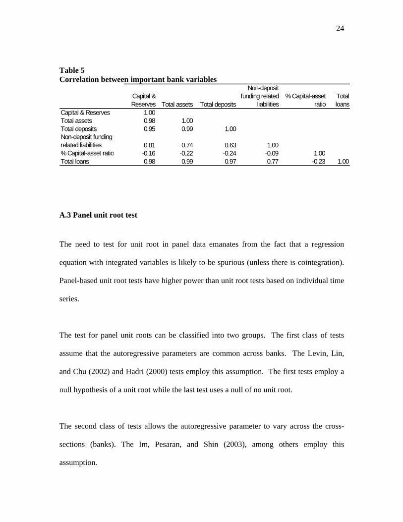
Table 5 Correlation between important bank variables

.3 Panel unit root test

root in panel data emanates from the fact that a regression

equation with integrated variables is likely to be spurious (unless there is cointegration).

Panel-based unit root tests have higher power than unit root tests based on individual time

series.

The test for panel unit roots can be classified into two groups. The first class of tests

assume that the autoregressive parameters are common across banks. The Levin, Lin,

and Chu (2002) and Hadri (2000) tests employ this assumption. The first tests employ a

null hypothesis of a unit root while the last test uses a null of no unit root.

The second class of tests allows the autoregressive parameter to vary across the cross-

sections (banks). The Im, Pesaran, and Shin (2003), among others employ this

assumption.

Capital & Reserves Total assets Total deposits

Non-deposit funding related

liabilities% Capital-asset

ratioTotal loans

Capital & Reserves 1.00Total assets 0.98 1.00Total deposits 0.95 0.99 1.00Non-deposit funding related liabilities 0.81 0.74 0.63 1.00% Capital-asset ratio -0.16 -0.22 -0.24 -0.09 1.00Total loans 0.98 0.99 0.97 0.77 -0.23 1.00

A

The need to test for unit

25

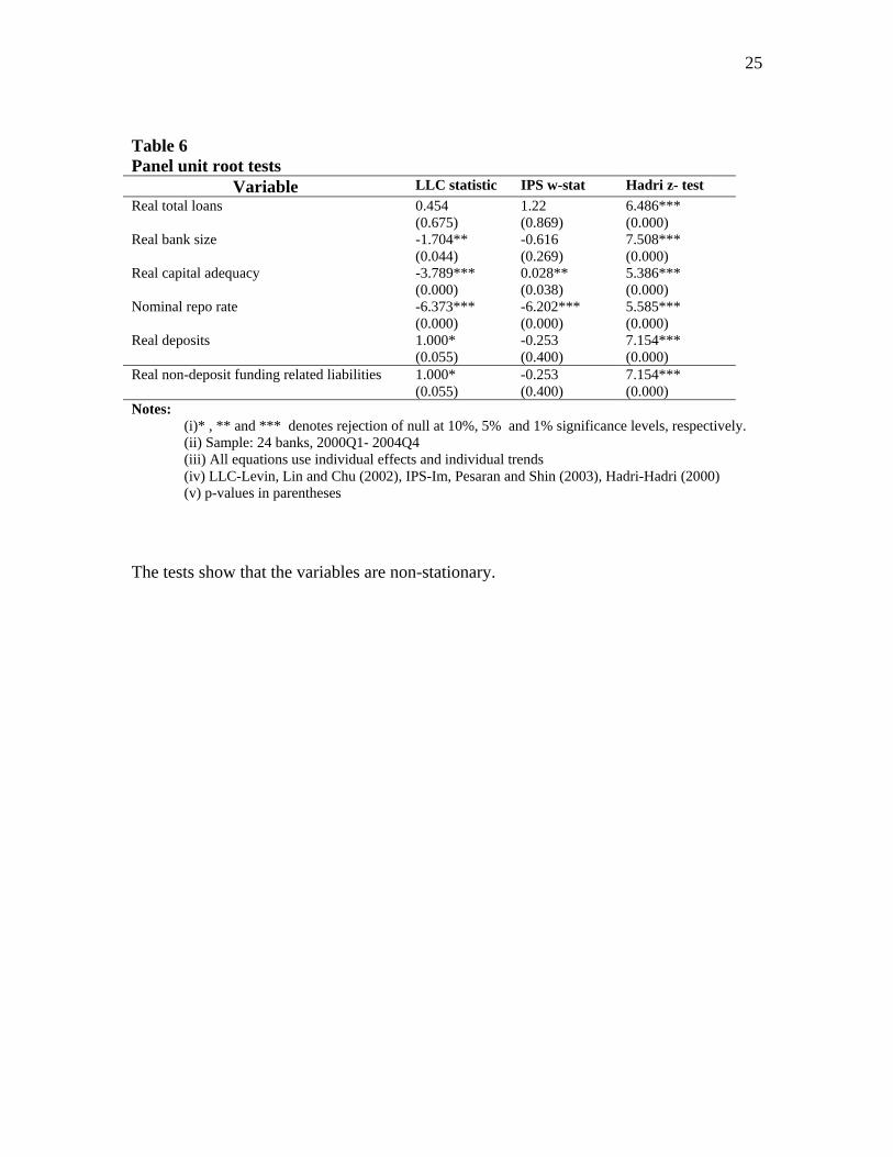
Table 6 Panel unit root tests

Variable LLC statistic IPS w-stat Hadri z- test Real total loans 0.454

(0.675) 1.22 (0.869)

6.486*** (0.000)

Real bank size -1.704** (0.044)

-0.616 (0.269)

7.508*** (0.000)

-3.789*** (0.000)

0.028** (0.038)

5.386*** (0.000)

Nominal repo rat)

Real non-deposit funding related liabilities

Real capital adequacy

e -6.373*** (0.000)

-6.202*** (0.000

5.585*** (0.000)

Real deposits 1.000* (0.055)

-0.253 (0.400)

7.154***(0.000)

1.000* (0.055)

-0.253 (0.400)

7.154***(0.000)

Notes: d *** denotes rejection of n 5% an cance pectively.

(ii) Sample: 24 banks, 2000Q1- 2004Qll equations use individual effect ividual tr

(iv) LLC-Levin, Lin and Chu (2002), I saran an 003), Ha 00)

The tes

(i)* , ** an ull at 10%, d 1% signifi levels, res4

(iii) A s and ind ends PS-Im, Pe d Shin (2 dri-Hadri (20

(v) p-values in parentheses

ts show that the variables are non-stationary.