Bank Structure and Entrepreneurial Finance:

Experimental Evidence from Small-Business Loans in India

Martin Kanz∗

Harvard University

This version: November 25, 2010

Abstract

This paper analyzes the effect of organizational structure on bank lending, using a framed fieldexperiment in the Indian market for small enterprise loans. The experiment varies the struc-ture of decision-making among participating loan officers by assigning authority over lendingdecisions to senior risk-managers or the bank’s front-line loan officers. Within this setting, Ishow that supervision adds substantial value, reducing defaults by 15 percent and increasingloan-level profit by 12 percent of the median loan size. This, however, comes at a cost: greaterhierarchical distance between the initial screener and the originator of a loan discourages boththe collection and use of qualitative information. Incentive contracts using performance pay toimprove the alignment of interests at different tiers of the bank’s decision-making process canmoderate these adverse effects. When loan officers and managers face identical performancepay, screening effort is unaffected, information communicated to supervisors is a more infor-mative predictor of default and loan-level profit increases by 24 percent of the median loansize. These findings shed new light on the nature and importance of agency conflict within thebank, and suggest that performance pay can play an important role in mitigating informationand agency problems in the provision of entrepreneurial finance in an emerging market.

Keywords: Banking, Entrepreneurship, Organizations, Development, Experiments

∗Contact: Department of Economics, Littauer Center, 1805 Cambridge Street, Cambridge, MA, 02138 USA. Phone:+1 (617) 230 8974. E-mail kanz@fas.harvard.edu. l thank Alberto Alesina, Shawn Cole, Andrei Shleifer and Jeremy Steinfor their guidance and support. I would also like to thank Ruchir Agarwal, Philippe Aghion, Oliver Hart, RajkamalIyer, Leora Klapper, Michael Kremer, Sendhil Mullainathan, Rohini Pande, Benjamin Schoefer, Raphael Schoenle,Antoinette Schoar, Vikrant Vig and seminar participants at Harvard and NEUDC 2010 for helpful comments andsuggestions. Financial support from the Paul Warburg Funds is gratefully acknowledged. Atul Agrawal and SamanthaBastian provided excellent research assistance. All remaining errors are my own.

1 Introduction

Theories of credit rationing have traditionally focused on information asymmetries between borrowers

and lenders (Stiglitz and Weiss 1981).1 More recent evidence suggests that agency conflict within the

bank can play an important additional role in limiting the provision of credit to informationally opaque

borrowers, such as small entrepreneurial firms (Liberti and Mian 2009, Hertzberg et al. 2010). Such

internal diseconomies may have far-reaching implications through their impact on the supply of credit.

However, empirical evidence remains scarce, due to the challenge of observing the internal dynamics

of a bank’s decision-making processes, and measuring their impact on risk-assessment and lending.

This paper uses a framed field experiment in the Indian market for small enterprise loans to

evaluate the effect of organizational design on incentives and decisions within the bank. Using a

novel experimental approach, I look directly into the black box of the underwriting process of small

enterprise loans in an emerging market and demonstrate that the structure of decision-making within

the bank has substantial effects on the collection, transmission and use of qualitative information.2

This affects credit decisions and constrains the profitability of lending. However, results from the

experiment also suggest that simple incentive contracts using performance pay to align the interests of

the initial screener and the originator of a loan are effective in attenuating moral hazard, facilitating

the flow of information, and improving the profitability of the bank’s lending.

In the experiment, loan officers from the staff of five Indian commercial banks evaluated credit

applications from a database of actual loans. The experiment randomized loan officers into three

treatments, which varied two features of the decision-making process: the assignment of formal au-

thority over the lending decision, and the alignment of monetary incentives between risk-managers and

subordinate loan officers.3 Lending decisions in the experiment were based on a sample of unsecured

small ticket loans, a leading example of a “character loan” for which the bank’s ability to incorporate

qualitative information into its decisions is especially important (Stein 2002, Berger et al. 2005). Since

the loans evaluated in the experiment had been previously made, their performance was observed and

1See also Jaffee and Russell (1976) and Leland and Pyle (1977). The literature on credit rationing in developingcountries is reviewed in Ghosh et al. (2000) and Karlan and Morduch (2009). Banerjee and Duflo (2008) show evidenceof credit constraints among Indian SMEs, suggesting high returns to capital in SME lending even in a comparativelydeveloped emerging financial market. See Djankov et al. (2007) and Beck et al. (2009) for evidence on private creditand financial access, Black and Strahan (2002), Cetorelli and Strahan (2006) and Kerr and Nanda (2009) on finance andentrepreneurship and King and Levine (1993) and Levine (2005) on finance and aggregate growth.

2The definition of qualitative or soft information follows (Petersen 2004) and defines qualitative information asinformation that has no direct quantitative equivalent and is either prohibitively costly or impossible to verify.

3The definition of formal authority used throughout the paper follows Aghion and Tirole (1997), who define formalauthority as the right, arising from a formal or informal contract, to decide over pre-specified matters. This idea alsorelates to the work of Grossman and Hart (1986) and Hart and Moore (1990), who focus on authority conferred bycontrol rights over an asset. The classification of the experiment follows Harrison and List (2004).

1

loan officers could be incentivized based on their decisions and the outcome of loans they approved.4

The idea that a bank’s organizational structure is integral to the nature and efficiency of its lending

finds indirect support in a large body of research on bank form and function. Using evidence from

the United States (Petersen and Rajan 1995, Berger and Udell 2002) and emerging markets as diverse

as Argentina (Berger et al. 2001) and Pakistan (Mian 2006), this literature shows that decentralized

banks tend to be more successful providers of financing to small, informationally opaque firms.5

The experimental approach used in this paper has three important features that allow me to shed

new light on the mechanisms underlying this general finding. First, by providing an unusually close look

into the underwriting process of small enterprise loans in an emerging market, the experiment makes

both effort and the flow of information inside the bank observable. Second, the experiment induces

exogenous variation in the structure of decision-making and the strength of managerial incentives.

This provides an ideal counterfactual for assessing the extent to which the structure of performance

pay can mitigate agency problems inside the bank (see Cole, Kanz, and Klapper 2010 for evidence

on performance incentives and lending). Finally, I observe the outcome of each evaluated loan, which

allows for the measurement and comparison of profitability under alternative organizational regimes.

The results of the experiment demonstrate that the organizational design of a bank’s lending affects

performance through two channels. On one hand, the shift towards a more hierarchical lending model

increases the probability that bad news about a borrower’s creditworthiness will be detected.6 Within

the context of the lending environment studied here, I demonstrate that this effect adds substantial

value from the bank’s perspective, increasing profit per loan by 12% of the median loan size. On

the other hand, as argued by Aghion and Tirole (1997) and Stein (2002), an increase in hierarchical

distance between the screener and the originator of a loan introduces a scope for agency conflict inside

the bank. This can affect performance by blunting incentives for the collection, transmission, and use

of relevant borrower information. I find compelling evidence for this incentive view of delegation, but

also show that these effects are mitigated by performance pay designed to more closely align incentives

within the bank; when loan officers and managers in the experiment faced identical performance pay,

effort remained unchanged, information transmitted to managers was a more informative predictor of

default and profit per loan was 24% higher than under delegated decision-making.

4In order to replicate the actual lending environment faced by loan officers in a commercial bank, the data underlyingthe experiment also included a subsample of loans that had been declined by the lender. Participating loan officers hadno previous indication about the quality of loans. As in the real lending environment, loan officers could be incentivizedonly on outcomes observable to the bank. On average, participants earned Rs 15,000 over the course of their participationin the experiment, which corresponds to approximately 60% of the median participant’s monthly wage.

5Mian (2006), shows, that recovery rates for delinquent loans in Pakistan are 28% higher among more decentralizeddomestic banks compared to their foreign competitors. Using data from banking mergers in the United States, Sapienza(2002) shows that when banks merge, the small-business lending of the combined organization declines.

6This is argument abstracts from the effect of organizational structure of incentives inside the firm and is akin tothe tradeoff between errors of commission and errors of omission illustrated in the work of Sah and Stiglitz (1986).

2

To guide the empirical analysis, I model the source of agency conflict inside the bank as an incomplete

contracting problem between the bank’s information-collecting loan officers and its senior managers. In

the model, as in the experiment, formal authority over the lending decision is exogenously assigned to a

senior manager or delegated to a subordinate loan officer, who may disagree about the optimal use of the

bank’s capital. The model illustrates how the structure of decision-making affects incentives inside the

bank and generates three testable predictions. First, supervision limits a reporting loan officer’s ability

to affect the bank’s final lending decision, thereby reducing incentives for the collection of information.

Second, the potential for disagreement between managers and loan officers also introduces frictions

in the transmission of relevant borrower information. Third, both of these effects are mitigated by

incentive contracts that improve the alignment of interests at the different levels of the bank’s corporate

hierarchy. The model thus highlights the tradeoff between the benefit of additional screening (a higher

probability that bad news about a borrower’s creditworthiness are detected) and the disincentive effects

of supervision, which arise from an increase in hierarchical distance between the initial screener and

the originator of a loan.

In the experiment, I test these predictions by means of three treatment conditions. These treat-

ments reflect salient features of lending models used in the Indian market for small enterprise loans, and

induce exogenous variation in the structure of the decision-making process. In the Baseline Treatment,

lending decisions were delegated to the bank’s front-line employees so that loan officers had full auton-

omy over the lending decision and could not be overruled by the intervention of a senior manager. In

the second treatment, the basic Supervisor Treatment, loan officers faced a senior manager who could

review and decline any loan suggested for approval. Managers in this treatment were more strictly

incentivized on the quality of their lending portfolio than their subordinates, and faced a penalty for

approving loans that subsequently became delinquent. The third treatment, the Aligned Supervisor

Treatment, is designed to distinguish the effect of supervision from the effect of divergent incentives

between employees at different levels of the bank’s corporate hierarchy, and matched the information-

collecting loan officer with a supervisor who faced identical performance incentives. By analyzing loan

officers’ effort, subjective assessment of credit risk and lending decisions under each treatment, I iden-

tify the nature of agency conflict inside the bank and quantify its effect on real outcomes, such as the

quality of lending decisions and loan-level profit.

Within this setting I establish three main findings on the importance, the nature, and the impact

of agency problems inside the bank. First, in line with incentive theories of delegation (Cremer 1995,

Aghion and Tirole 1997, Stein 2002) I show that the shift towards a more hierarchical lending model

blunts incentives for the collection of information. Loan officers who were matched with a supervisor

3

spent 7% less time reviewing each proposed loan. This effect disappears when monetary incentives at

the two levels of the bank’s corporate hierarchy are more closely aligned. When information-collecting

loan officers and loan-approving managers face identical monetary incentives, screening effort increases

by up to 9%, relative to the Supervisor Treatment and is statistically indistinguishable from effort under

the Baseline Treatment, which delegated lending decisions to the bank’s loan officers.7

Second, I use internal credit ratings to measure how the structure of decision making affects incen-

tives for the transmission and use of qualitative information. I find that the misalignment of monetary

incentives between reporting loan officers and loan approving managers leads to substantial frictions in

the transmission of qualitative information. While reported credit ratings are an informative predictor

of default even when final lending decisions are not made by the information producing loan officer (a

one standard deviation improvement in a loan’s overall risk rating is associated with a 10% decrease in

the probability of default), risk ratings become a significantly more informative predictor of default as

monetary incentives between the two tiers of the bank’s corporate hierarchy are more closely aligned.

Third, the effect of hierarchical distance on the bank’s ability to incorporate qualitative information

into final lending decisions is more nuanced: While managers’ decisions do not respond to risk ratings

passed on by reporting loan officers under basic supervision, several sub-components of the qualitative

risk rating –including business and management risk– retain their ability to affect final lending decisions

when the gap in performance pay between loan officers and risk managers is reduced.

What is the effect of these observed distortions on outcomes and performance? Having established

that the structure of decision making inside the bank affects incentives to acquire, share and use

information, I demonstrate that these distortions affect the quality of lending decisions and loan-level

profit. The results show that in the setting of the experiment, the benefit of supervision outweighs

the costs of agency conflict induced by greater hierarchical distance. Profits per loan increase by $266

(12% of the median loan size) relative to the Baseline Treatment when lending decisions are made

in a hierarchy. However, the results also demonstrate that disincentives for the collection and use of

qualitative information constrain the profitability of the bank’s lending. I show that when incentives

at the two levels of the bank’s corporate hierarchy are aligned, subordinate loan officers are 12% less

likely to recommend non-performing loans and loan level profit is $516 (24% of the median loan size)

higher than when decisions are delegated to the bank’s front-line loan officers.

These results have important implications for the design of lending models in emerging markets,

7It is worth noting that the observed relationship between incentive alignment and effort also speaks against anexplanation based on moral hazard in teams (Alchian and Demsetz (1972), Holmstrom (1982), see also Bandiera,Barankay, and Rasul (2010) for related empirical evidence from a field experiment). If loan officers were tempted tofree-ride, we would expect effort to decrease, when supervisors are incentivized to exert greater screening effort.

4

where the provision of entrepreneurial finance promises high returns to capital, but small businesses

often lack collateralizable wealth and a documented history of formal sector borrowing. In 2009, less

than 10% of small businesses in India were covered by a credit bureau report (World Bank, 2010). This

implies high information costs, which are often cited to explain why commercial lending in emerging

markets tends to be heavily skewed in favor of large corporate loans for which standard hard information

is more reliable. My results demonstrate that in this environment, the organizational design of a bank’s

lending plays a crucial role in shaping incentives for the collection and use of qualitative information

and determining the bank’s ability to screen borrowers and provide credit.

The results presented in this paper complement the existing empirical literature on agency prob-

lems in banks (Liberti 2003, Liberti and Mian 2009, Agarwal and Wang 2009, Hertzberg et al. 2010)

and incentives within firm more broadly (Lazear 2000, Bandiera, Barankay, and Rasul 2007, 2009,

Paarsch and Shearer 2009, Bandiera, Barankay, and Rasul 2010). By suggesting a causal mechanism

that can rationalize the observation that decentralized banks are better providers of finance to small

entrepreneurial firms (Petersen and Rajan 1994, Boot 2000, Berger and Udell 2002, Mian 2006), this

paper also relates to the literature on bank function and organizational design (Berger et al. 2001,

Berger and Udell 2002, Petersen and Rajan 2002, Berger et al. 2005, Mian 2006).8

On the theoretical side, this paper relates most directly to the literature on incentive theories of

delegation (Aghion and Tirole 1997, Stein 2002). In contrast to traditional theories of monitoring, the

models in this literature argue that supervision reduces the agent’s ability to affect the decisions of

the firm (the lending decision in the context studied here) and therefore blunts incentives at the lower

levels of the corporate hierarchy. Thus, within this framework, an important rationale for delegating

authority in a bank is to strengthen incentives for the acquisition and use of qualitative information.

The experiment allows for a direct test of these propositions.

The remainder of the paper proceeds as follows. Section two provides context about the Indian

market for small enterprise loans in which the experiment is set, and describes the financial product

on which lending decision in the experiment were based. In section three, I develop a stylized model of

the screening process to motivate the subsequent empirical analysis. Section four provides an outline

of the experimental design and method of randomization. Section five provides descriptive statistics

on the participant pool and sample of loans used in the experiment. Section six presents the empirical

results and section seven concludes.

8In terms of methodology, this paper also relates to recent work by Gine, Jakiela, Karlan, and Morduch (2010) andFischer (2010) who use framed field experiments to study risk-taking and credit decisions in a microfinance context.

5

2 Environment: Small Enterprise Lending in India

The experiment is set in the market for unsecured small enterprise loans in India. With an estimated

30 million micro-enterprises and SMEs, accounting for 22% of GDP and 12% of net bank credit,

India’s market for entrepreneurial finance ranks among the largest in the world.9 However, financing

constraints remain pervasive and represent an important limiting factor to the growth and entry of

small businesses (Banerjee et al. 2003, Banerjee and Duflo 2008). Despite a long history of directed

lending programs requiring commercial banks to extend up to 40% of total credit to agriculture and

small-scale industry, fewer than 15% of registered small enterprises in India currently have access to

institutional credit (Government of India, 2010).

The analysis in this paper studies lending decisions based on a database of previously evaluated

loans, compiled in collaboration with a leading commercial lender (hereafter “the Lender”). The loans

are described in greater detail in section 5.2 below. The Lender is one of India’s largest providers of

mass-market finance and competes in the market for small enterprise loans through a network of more

than 700 local branches across the country. The Lender’s small enterprise product range caters to firms

with limited access to the formal credit market due to collateral constraints, or with turnover below

the amount required to qualify for a working capital loan or a revolving line of credit. These loans are

given in the name of an individual rather than the corporate entity, making them a more accessible

source of financing for start-ups and small businesses with limited access to institutional credit.10

To ensure consistency in the type of loans used in the experiment, I focus on unsecured small

enterprise loans to self-employed individuals with a ticket size between Rs 100,000 (approximately

$2,000) and Rs 500,000 (approximately $11,000). The median loan size in my sample is Rs 150,000

($3,325), and corresponds to 31% of the average client’s annual net income. Loans in this market are

generally fixed-installment term loans with a maturity of 12 to 48 months and interest rates between

20 and 35% annual percentage rate (APR). Typical uses of this type of loan include the financing of

overhead, small investments and the repayment of higher-interest-rate loans from the informal sector.

Prospective borrowers are sourced and screened by the Lender’s local branches, which collect all

9The classification follows the Reserve Bank of India which defines medium enterprises as firms with less than Rs 10(approximately $200,000) million investment in plants and machinery and small industries as firms with fixed investmentin plant and machinery of below Rs 5 million (approximately $100,000).

10The larger ticket size and limited observability of cash-flows of the loans considered here generally rules out the use ofjoint-liability contracts that have facilitated the extension of microfinance to marginal borrowers, see also de Aghion andMorduch 2005. Broadly comparable products are offered by several commercial lenders in the Indian market. BecauseIndia strictly regulates branch banking (see also Burgess and Pande 2005), many private lenders operate as Non-BankingFinancial Companies (NBFCs). NBFCs are not allowed to take demand deposits and face limitations in the type ofloans they can provide. NBFC can, for instance, give small business term loans to self-employed individuals but are notallowed to provide commercial loans to corporate entities.

6

required documentation, including a client’s bank statements and tax returns and check whether the

client has a credit bureau report (available for 60% of clients in my sample). Additionally, the Lender

solicits three independent trade references and verifies some of the provided information through a

site visit to the client’s business. Lending decisions for uncollateralized loans are largely based on

estimated cash flows, and approximately 30% of prospective clients are screened out at this stage.

While none of the loans in the experiment carried any collateral security, borrowers faced strong

incentives for repayment. First, the Lender routinely offers follow-up loans at reduced interest rates to

clients with a good repayment history. Second, borrowers who default on their loans are reported to

India’s main credit bureau, implying a credible threat of future exclusion from formal sector borrowing.

This is especially salient given that for most firms interest rates on these loans –while high by formal

sector standards– are significantly below the cost of alternative sources of financing. As a result, default

rates are below 5%, which is above the figure for regular commercial loans, but much lower than default

rates observed for other uncollateralized products targeting clients with limited financial access.11 The

Lender classifies loans as delinquent if a client misses more than two monthly payments and remains

60+ days overdue. Loans that remain unsettled for 90+ days are classified as non-performing assets

(NPA), reported to the credit bureau, and referred to the Lender’s collections department. A small

fraction of loans in the overdue category are restructured in direct negotiation between clients and the

Lender. To rule out selection bias, the sample excludes repeat borrowers and restructured loans.

The choice of product was guided by several considerations. First, an unsecured small business

loan is a prime example of a “relationship loan” with a comparatively low level of documentation. The

cash flow of small businesses is generally difficult to verify, and audited financials often reflect only

part of the applicant’s true financial position. In this environment, the lending decision relies heavily

on the lender’s ability to incorporate “soft information” into the lending decision. Second, covenants

for this class of loan have no provisions for review or ex-post adjustments in the terms of lending. This

means that risk management occurs primarily through screening at the time the loan is sanctioned

(passive monitoring), rather than follow-up once a loan has been originated (active monitoring).12

This ensures that the performance of a loan reflects a borrower’s actual credit risk, rather than ex-post

modifications to the terms of lending. Third, the Reserve Bank of India, which regulates lenders in this

market, closely prescribes the type of borrower information a lender is required to collect for this class

of loan. Thus, while products in this market are somewhat differentiated across banks, loan officers

11Karlan and Zinman (2009) and Bertrand et al. (2010) carry out experiments in the South African market for cashloans and report default rates between 15% and 30%. The loans used as a basis for the experiment reported in thispaper have a much larger ticket size, are longer maturity and cater to a segment of with significantly lower default risk.

12The distinction between active and passive monitoring is common among practitioners and in the literature, see forexample Hertzberg, Liberti, and Paravisini (2010)

7

in the experiment were able to base lending decisions on information that was largely standardized,

as mandated by the regulator. As a further motivation for the experimental treatments, it is worth

noting that, while the market segment I study is served by a range of private and public sector lenders,

there are important differences in the lending models. At public sector banks, the lending decision for

personal and small enterprise loans up to a given ticket size tends to be delegated to local branches,

such that sales and credit assessment roles may coincide. Among private sector lenders, in contrast,

sales and credit assessment roles are generally distinct and the lending decision tends to be centralized.

3 Theoretical Framework

To guide the empirical analysis, this section develops a stylized model of the underwriting process.

I describe a sequential version of the Aghion and Tirole (1997) model of incentives inside the firm,

which provides a number of testable implications. The model takes the benefit of additional screening

–a greater probability that bad news about a borrower’s creditworthiness are detected– as given and

focuses on sources of agency conflict within the bank that can be identified in the empirical analysis.

In the model, a loan officer (agent) and a risk manager (principal) are employed by the bank to

screen loans. All loans look ex-ante identical and the problem facing loan officers and risk managers

is to choose costly screening effort to differentiate between borrowers. Because the bank does not

observe borrower type, incentive contracts can be based only on the observable outcome of loans that

have been approved. The bank has limited capital and principal and agent may disagree over what

type of loans to make. Specifically, due to limited liability, the agent may have a lower threshold for

approving loans than a senior manager.13 The principal, on the other hand, is more concerned about

overall portfolio quality and may prefer to decline marginal loans so that the bank’s capital may be

deployed elsewhere at a higher return. The model illustrates how such scope for disagreement shapes

incentives for the collection, transmission and use of qualitative information.

The model abstracts from the experimental set-up by assuming that the principal, rather than

merely deciding whether to approve or decline a loan, has discretion over allocating the bank’s capital

to a recommended loan or an alternative project. The model additionally simplifies the setting of

Aghion and Tirole (1997), by assuming that when lending decisions are delegated the principal is not

involved in the lending decision, such that the agent is entirely autonomous in her decision-making.

13In an actual lending environment, such a divergence of interests is rather common and may arise from varioussources, such as limited liability, career concerns (Gibbons and Murphy 1992), differences in time horizons, discountrates and monetary incentives between loan officers and risk-managers. The model is agnostic about the source ofdivergent interests. The experiment exogenously induces an incongruence a divergence in interests by varying the powerof monetary incentives faced by principal and agent and hence their quality threshold for loan approval.

8

3.1 A Simple Model of Credit Screening

Two agents, a risk manager (principal) and a loan officer (agent), indexed by i ∈ {P,A} are employed

by the bank to screen N loans. The problem facing principal and agent is to choose screening effort,

infer the quality of a loan and make a profitable lending decision. At the beginning of the game, and

before any screening takes place, the bank exogenously assigns formal authority, defined as the right

to make a final lending decision, to either the principal or the agent.

3.1.1 Sequence of Play

1. The bank exogenously assigns authority over lending decisions to the principal or the agent.

2. Principal and agent privately and sequentially gather information about loan quality.

3. If formal authority is assigned to the agent, the agent screens loans without the principal’s

interference. If formal authority is assigned to the principal, the agent may recommend a loan for

approval and additionally disclose non-verifiable information about loan quality to the principal.

4. The party holding formal authority makes a final and irreversible lending decision. Loan perfor-

mance is observed and payoffs are realized.

3.1.2 Loans

Each loan is associated with an ex-ante unknown but ex-post verifiable benefit B for the principal and

b for the agent. A loan made by the principal yields benefit θB to the agent and a loan suggested by

the agent yields benefit θb to the principal. For simplicity, suppose that N loans are screened, but only

two of these loans are relevant so that one loan yields benefit B > 0 to the principal and the other

yields zero. Similarly, one loan yields benefit b > 0 to the agent and the other yields zero. The ex-ante

probability that principal and agent agree in their assessment and prefer to approve the same loan is

denoted by θ ∈ (0, 1], the parameter of congruence. The experimental treatments, which I describe in

the next section, allow me to induce exogenous variation in this parameter.

3.1.3 Information and Screening

At the beginning of the game, all loans look identical and principal and agent must collect information

to differentiate between them. If the agent exerts screening effort e ∈ [0, 1) at private cost c(e), he

learns his expected benefit with probability e and remains uninformed with probability 1−e. Similarly,

if the principal exerts screening effort E ∈ [0, 1) at private cost c(E), she becomes informed about her

9

benefit from approving the loan with probability E and remains uninformed with probability 1 − E.

For both principal and agent, the payoff from approving a bad loan is sufficiently negative that an

uninformed party will always prefer to decline a loan. This corresponds to the prior that the average

loan in the population yields a negative payoff, so that it is never optimal to approve a loan when

the screening process does not reveal any information about borrower type. When no loan is made,

principal and agent earn the outside payments B = b = 0. As an extension, which allows me to

investigate the effect of incentive alignment on communication, I also consider the case in which an

informed agent can disclose information he may hold about the quality of the loan to the principal.

3.1.4 Preferences

For simplicity, I assume that principal and agent are risk-neutral, so that for a given level of effort

and implemented lending decision, the agent’s expected utility is uA = b − c(e) and the principal’s

expected utility is uP = B − c(E). To further simplify the exposition, and without loss of generality,

I assume that effort entails disutility c(E) = 1/2 E2 for the principal, and c(e) = 1/2 e2 for the agent,

respectively.

3.2 Screening Effort and Lending Decisions

3.2.1 Lending decisions under delegation

To motivate the Baseline Treatment in the experiment, consider first the case in which formal authority

over the lending decision is delegated to the agent, who screens loans without the interference of

a supervisor.14 The agent exerts screening effort, which comes at private cost 12e

2 and learns his

expected benefit from approving the loan with probability e. With probability 1−e, the agent remains

uninformed, declines the loan and earns outside wage b = 0. Thus, the agent’s expected utility is

uA = eb− 12 e

2 (1)

and the agent’s choice of effort is e∗d = b. Hence, when lending decisions are delegated, the agent

chooses his privately optimal effort level e∗d and makes a decision without the principal’s interference.

14Note that this implies that, as in the empirical lending environment I study, a supervisor can overrule a subordinateonly on a positive, but not a negative recommendation. This is a departure from Aghion and Tirole (1997), who assumethat an agent who remains uninformed solicits and follows the principal’s assessment.

10

3.2.2 Lending decisions under supervision

How are incentives to collect information affected when lending decisions are made in a hierarchy? To

match the experimental design and empirical lending environment, I next consider the case in which

loans are screened sequentially by the principal and the agent. All loans are first screened by the

agent. With probability e, the agent is informed and can make a recommendation. With probability

E, he faces a principal who is informed and makes a decision, yielding benefit θB to the agent. With

probability 1 − E, however, the agent faces a principal who is uninformed and therefore optimally

follows (rubber-stamps) the agent’s suggestion, yielding benefit b to the agent. With probability 1− e

the agent remains uninformed and earns b = 0. Thus, the agent’s expected utility under supervision is

uA = e(EθB + (1− E)b

)− 1

2e2 (2)

When a loan is recommended by the agent for approval it is reviewed by the principal. As in the

experiment and the empirical lending environment, the principal reviews only loans not previously

screened out by the agent (that is, the mass of loans e).15 With probability E the principal learns his

benefit from making the loan, makes a lending decision and earns payoff B. With probability 1 − E,

the principal learns nothing, optimally follows the agent’s suggested decision and earns θB. Thus, the

principal’s expected utility is

uP = e(EB + (1− E)θb− 1

2E2)

(3)

As is intuitive, in this setting, principal and agent choose effort strategically. I consider a Perfect

Bayesian Equilibrium of this game, which rules out the possibility that an agent exerts no screening

effort and recommends all loans for approval. In this case, the first order conditions that follow from

(2) and (3) define the principal’s and the agent’s reaction curves for information gathering and have a

unique intersection.

E∗s = B − θb (4)

e∗s = E(θB − b) + b (5)

These conditions make a number of intuitive predictions. First, the principal supervises more when

her stake is high and the congruence parameter θ is low, so that she is likely disagree with the agent’s

decision. Second, the agent’s initiative is decreasing in the principal’s monitoring effort E. This

15This structure of decision making is rather common in retail lending and corresponds to the case where sales andapproval channels are separate and loans declined at the branch level are not sent to the bank’s credit department forreview.

11

property of the model illustrates the disincentive effect of supervision. The intuition for this result is

straightforward. Whenever there is scope for disagreement between the principal and the agent, an

increase in the principal’s monitoring effort makes it more likely that the agent’s decision is overturned.

This, in turn, reduces the agent’s expected return from exerting effort and collecting relevant borrower

information. Third, when θ = 1, so that there is no scope for disagreement between principal and

agent, the agent exerts optimal screening effort and the principal’s screening effort goes to zero such

that she always trusts and rubber-stamps the agent’s decision.

The model thus generates the following testable predictions, describing the effect of organizational

structure on loan officers’ incentives to acquire information.

Proposition 1 (The Disincentive Effect of Supervision) The agent exerts less effort under supervision.

This follows directly from a comparison of (2) and (6), which shows that[E(θB−b)+b

]≤ b and hence

e∗s ≤ e∗d for all E > 0 and θ < 1. Proof: see Appendix A.

Proposition 2 The agent invests greater effort in gathering information when her preferences are

more closely aligned with those of the principal: ∂e∗s/∂θ > 0. Proof: see Appendix A.

Note that this basic framework also makes reduced-form predictions about the use of qualitative

information communicated by reporting loan officers. As the interests of principal and agent become

more closely aligned, and θ approaches one, the principal reduces her monitoring effort (∂E/∂θ < 0).

This implies that an agent’s positive recommendations are less likely to be overturned and information

collected by a reporting loan officer is more likely to affect the bank’s ultimate lending decision. Finally,

this also implies that an increase in the potential for conflict between the different layers of the bank’s

corporate hierarchy induces frictions that reduce the volume of lending –as any loan recommended

for approval is more likely to be turned down. As we shall see, results from the experiment provide

evidence consistent with these two additional empirical predictions.

3.2.3 Communication

The model can also shed light on the effect of organizational structure on incentives to communicate

information about a potential borrower’s credit risk. To see this, I introduce the possibility that

agents can disclose private (non-verifiable) information to the principal, which reduces the principal’s

marginal cost of investigation to ∂cc(E)/∂E < ∂c(E)/∂E for any level of monitoring effort E > 0.

This leads to a shift in the principal’s reaction curve and increases the principal’s monitoring effort.

In the experiment, I operationalize this idea by allowing loan officers to send an internal, non-verifiable,

12

risk rating to their manager. The availability of this additional information might be thought of as

allowing the manager to target any additional screening effort towards a salient subset of information

contained in a client’s loan file. In this way, the experiment makes communication observable and

allows me to test the following prediction.

Proposition 3 (Communication) The agent discloses more information when incentives with the

principal are more closely aligned. Proof: see Appendix A.

The intuition for this result is straightforward. When the interests of principal and agent are mis-

aligned, denoted by a low congruence parameter θ, an agent who shares private information increases

the risk of being overruled by an informed principal. By contrast, when the interests of principal and

agent are aligned, the agent benefits from sharing information with the principal, as a principal with

aligned interests (high θ) is likely to implement the agent’s preferred decision.

3.2.4 Testable implications

The model gives rise to the following testable predictions. First, relative to the baseline case of

decentralized decision-making, the observable effort of reporting loan officers should decline under

supervision. Second, in a hierarchy, the screening effort of loan officers is increasing in the degree

of incentive alignment with their senior managers. Third, loan officers will disclose more private

information about proposed loans when their incentives are more closely aligned with those of the

loan approving managers. Finally, when congruence between loan officers and risk managers is high,

managers monitor less and are therefore more likely to follow the agent’s recommended decision.

To test these predictions, the experimental treatments vary (i) the allocation of formal authority

over the lending decision and (ii) the structure of performance pay inside the bank. In order to identify

the sources of agency conflict highlighted in the model, I vary the congruence parameter θ by altering

the alignment of performance pay between loan officers and senior managers.

In the experiment, loan officers and risk managers were awarded the conditional payments ai for

loans that were approved and performed, bi for loans that were approved and subsequently became

delinquent and a payment ci for loans that were declined. Hence, upon observing an informative signal

about a borrower’s creditworthiness, the decision rule for approving a loan is given by piai+(1−pi)bi ≥

ci,16 where pi denotes the expected probability of performance. This simply states that a loan officer

will approve a loan if her expected benefit from making the loan is greater than the outside payment

16Throughout the paper, I assume that loan officer’s prior about the average loan in the population is such thatloan officers and managers will always prefer inaction to approving a loan when no information about a borrower’screditworthiness is obtained from the screening process.

13

ci, which is made if the loan is declined. This decision rule defines a threshold probability for loan

approval as a function of the incentive parameters for loan officers pa(aa, ba, ca) and senior managers

pp(ap, bp, cp), respectively. In the experiment, I alter the incentive payments faced by loan officers

and supervising risk-managers, such that interests between reporting loan officers and loan approving

managers are either aligned (θ = 1) and pa = pp or divergent (θ < 1) and pa < pp.

Finding evidence consistent with the predictions of the model would, first, provide support for the

hypothesis that a bank’s ability to screen borrowers is constrained by the presence of agency conflict

inside the firm and, second, shed light on the interaction between performance pay and organizational

structure in shaping firm performance. While any incentive contract observed in an empirical lending

environment is likely to be endogenous to the firm’s performance (Bandiera et al. 2007, Prendergast

1999, Chiappori and Salanie 2003), the experimental design used here allows me to induce exogenous

variation in the structure of decision-making, thus allowing for an identification of causal effects.

4 The Experiment

4.1 Basic Setup of the Intervention

In the experiment, 125 loan officers, drawn from the staff of five commercial banks evaluated loan ap-

plications from a database of 325 loans, assembled in cooperation with a large commercial lender. The

exercise was carried out at two dedicated experimental labs in the western Indian city of Ahmedabad

between May and August 2010, and participants completed a total of 3, 042 lending decisions over the

course of the experiment.

Loan officers invited to participate in the experiment were recruited in cooperation with the regional

offices of five commercial banks. Individuals identified by these partner institutions were contacted

by a member of the local lab staff and invited to attend an introductory presentation to familiarize

themselves with the exercise and experimental protocol. Loan officers who agreed to participate were

then contacted on a weekly basis to arrive at the lab at a pre-arranged time to complete an experimental

session. Summary statistics for the pool of participants appear in Table 1.

When participating loan officers arrived at the lab, they were randomly assigned to one of three

experimental treatments, under which they evaluated a set of six loan applications per session. Ran-

domization was carried out at the loan officer and session level to ensure a sequence of treatments

orthogonal to loan officer characteristics, treatment type and composition of the participant pool. The

loan files assigned to each loan officer were randomly and independently drawn from the database of

14

historical loans, subject to the constraint that no officer would be assigned the same file more than

once. To add to the realism of the lending environment, loans shown to participants included loans

that had performed, loans that had defaulted and loans that had been declined by the Lender.17 Par-

ticipants knew that they were evaluating actual loans, but had no information on whether a loan had

been previously made by the Lender.

Each session of the experiment began with a standardized one-on-one presentation by the lab

administrator, introducing the loan officer to the assigned treatment. Each treatment varied two

features of the decision-making process: the assignment of decision rights to either principal or agent

and the performance pay faced by the two parties. The participants were briefed on these features

according to a standardized protocol and completed a short quiz to verify their understanding of the

treatment prior to beginning the exercise.

Participants were then logged into a customized software interface (see Figure 6 for a screenshot),

which displayed the randomly assigned sequence of loan files. The information for each loan consisted

of the complete pre-sanction documentation, as available to the Lender at the time the original lending

decision was taken. Participants were able to go back and forth between the different sections of the

credit file and faced no time constraint in completing the exercise. After reviewing this information,

loan officers were then asked to assess the credit risk of each applicant along eighteen rating criteria,

grouped into the categories personal risk, management risk, business risk and financial risk. In the

last step, participants then decided to approve or decline the loan.18 Throughout the experiment, a lab

administrator was available to answer questions and ensure that there was no communication among

the participants during the exercise.19

In a subset of experimental treatments, participants were randomly assigned to play the role of a

supervisor. In this setting, a subordinate loan officer (agent) was able screen out loans, which were

then not reconsidered by the risk manager (principal), but did not have the authority to approve a

loan. Thus, a supervisor was able overrule a subordinate on positive, but not on negative lending

decisions. This corresponds to the common practice in the real lending environment I study where,

for instance, loans declined at the branch level are not passed on to the bank’s credit department for

a second assessment.

17The ratio of performing, non-performing and declined loans was kept constant throughout the exercise at 4 per-forming, 1 non-performing and 1 declined loan per session. This ratio corresponds to the ratio for comparable loans atcommercial banks in India and was not disclosed to the participants. In separate robustness checks, I test for learningduring the exercise and check whether lending decisions approached the population ratio of good and bad files but findno evidence that participants learned to infer the ratio of good to bad files over the course of the exercise.

18The internal risk ratings assigned during the exercise were not binding, such that participants were free to approveor reject a loan irrespective of the assigned rating.This corresponds to the standard practice in the market I study, whereloans to firms with a turnover of less than Rs 1,000,000 receive an internal credit rating, but the lending decision is notbased on a formal credit scoring model.

19All lab administrators were employees of Ahmedabad Office of the Center for Microfinance.

15

Throughout the experiment, participants faced meaningful monetary incentives based on their lending

decisions and the outcome of the loans they approved. To ensure that monetary stakes were perceived

as meaningful by the participants, the average payment was calibrated to approximately twice the

hourly wage of the median loan officer. Participants received a show-up fee of Rs 100 (approximately

$2.15) and a performance bonus of up to Rs 300 (approximately $6.45) awarded at the end of each

experimental session.20

4.2 Experimental Treatments

I implement three experimental treatments, summarized in Table A below. The treatments vary, first,

the assignment of formal authority over the lending decision to either a risk manager (principal) or

loan officer (agent) and, second, the alignment of monetary incentives between the two parties.

To induce exogenous variation in the probability threshold for accepting a loan pi, the experimental

treatments alter the structure of performance pay faced by loan officers and risk-managers. I vary the

pa. Each treatment specified three contingent payoffs for loan officer and manager, conditional on

the final lending decision and the outcome of loans that were approved. These payoffs distinguished

between a payment a for a loan that was approved and performed, a payment b, for a loan that was

approved and became delinquent and a payment c, for a loan that was declined. To facilitate notation,

I denote these payments by the triple (ai, bi, ci). Throughout the experiment, loan officers faced the

incentive scheme (20, 0, 10), while risk managers faced either identical monetary incentives (20, 0, 10)

or more high-powered performance pay, which carried a penalty for approving loans that subsequently

became delinquent (50,−100, 10).21 The first combination of incentive payments corresponds to the

case of congruent interests and identical thresholds for approving a loan pa = pp, the second combina-

tion of incentive payments corresponds to the case of misaligned incentives and pa < pp. In this latter

case, a loan-approving manager is more stongly incentivized on the quality of loans she originates than

the reporting loan officer, which implies a higher quality threshold for approving a loan.

As in the empirical setting, loan officers could be incentivized only based on outcomes that were

observable to the bank. All incentive payments, as well as the show-up fee, were awarded by the lab

administrator after the de-briefing which concluded each session of the experiment.22

20Whenever lending decisions were made by a hierarchy, consisting of a loan officer and a risk-manager, all performancepay was conditional on the lending decision of the manager, who held formal authority over the lending decision. Thiscaptures the fact that, as in the empirical setting, the bank only observes the outcome of loans that are approved.

21As in the empirical setting, loan officers could be incentivized only based on outcomes that were observable to thebank. Therefore, whenever a loan was declined at any level of the screening process, both parties received payoff c. Thismeant that a loan officer who suggested a loan for approval which was subsequently turned down by the manager wasnot rewarded for a correct recommendation, since the outcome of the loan was not observed by the bank. Similarly, if aloan was screened out by the agent, both parties received the payment c.

22In the de-briefing participants also received feedback on the accuracy of their lending decisions and were shown a

16

4.2.1 The Baseline Treatment

This treatment was assigned to 107 loan officers, covered a total of 1,629 lending decisions and serves

as the benchmark for all comparisons throughout the experiment. Under the Baseline Treatment, loan

officers were given complete autonomy over the lending decision. Participants were able to review

all information contained in a prospective client’s credit file, provided a qualitative assessment of the

applicant’s credit risk and made a decision to approve or decline the loan.

4.2.2 The Supervisor Treatment

With this treatment, which was assigned to 102 participants and covered a total of 786 lending de-

cisions, I test Proposition 1 of the model. The model predicts that, as a loan officer loses influence

over the final lending decision, incentives for the acquisition of information are blunted. Hence, for

any value of the congruence parameter θ < 1, the agent’s effort under supervision will be lower than

the agent’s effort in the Baseline case of decentralized decision making.

In the Supervisor Treatment, formal authority was exogenously assigned to a senior manager.

Participants assigned to this treatment were aware that their recommended lending decisions would

be reviewed by a manager with the authority to overrule their recommendation. The decision making

process under the Supervisor Treatment proceeded as follows. Loan officers were presented with a

sequence of randomly assigned loan files. They provided a qualitative risk assessment and were able

to either decline a loan or forward it to the manager for approval. For any loan that arrived at the

risk-manager’s desk with a loan officer’s recommendation to approve, the risk manager had access to

all hard information contained in the loan file, and was additionally able to review soft information

in the form of the subordinate loan officer’s qualitative assessment of the client’s credit risk. As in

the real lending environment I study, loans screened out by the bank’s front-line loan officers were not

reconsidered at higher levels of approval.

4.2.3 The Aligned Supervisor Treatment

This treatment is designed to test Proposition 2 of the model. The model shows that, the alignment

of incentives between principal and agent increases the probability that a reporting loan officer’s

recommendation will be followed, thus mitigating the disincentive effect of supervision (∂e/∂θ > 0).

The Aligned Supervisor Treatment was assigned to 96 loan officers and covered a total of 627

lending decisions. The protocol for this treatment was identical to the Supervisor Treatment, with the

scorecard comparing their decisions against the observed ex-post performance of each loan.

17

exception that the introductory briefing emphasized that loan officers now faced a supervisor whose

monetary incentives were aligned with their own. In practical terms, this meant that, in contrast to

the previous treatment, the risk manager was not penalized for approving a loan that subsequently

became delinquent.

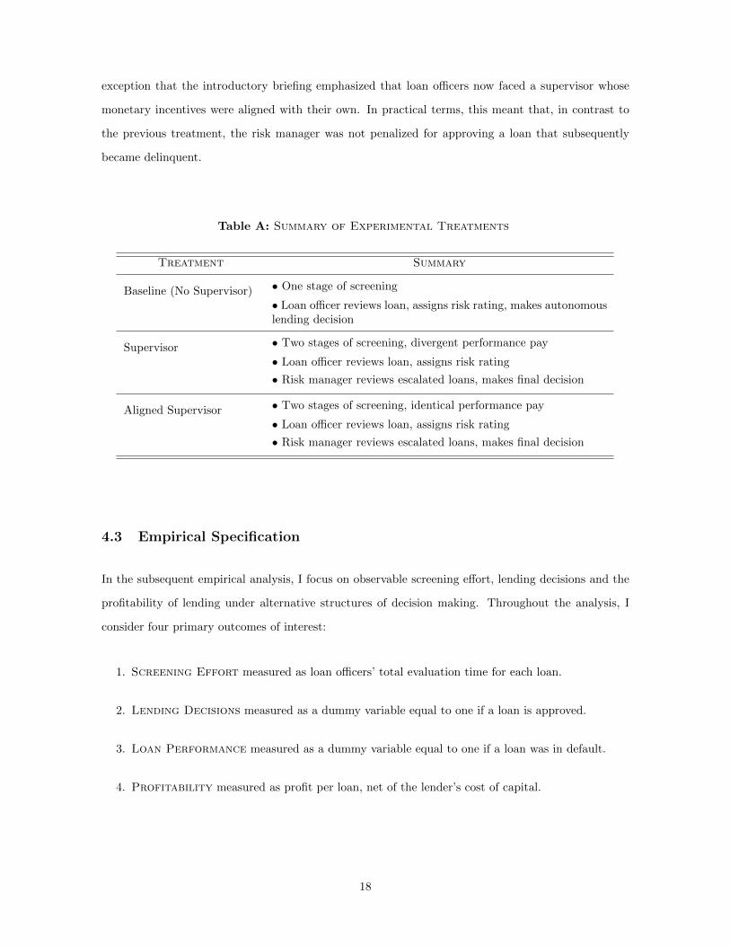
Table A: Summary of Experimental Treatments

Treatment Summary

Baseline (No Supervisor) • One stage of screening

• Loan officer reviews loan, assigns risk rating, makes autonomouslending decision

Supervisor • Two stages of screening, divergent performance pay

• Loan officer reviews loan, assigns risk rating

• Risk manager reviews escalated loans, makes final decision

Aligned Supervisor • Two stages of screening, identical performance pay

• Loan officer reviews loan, assigns risk rating

• Risk manager reviews escalated loans, makes final decision

4.3 Empirical Specification

In the subsequent empirical analysis, I focus on observable screening effort, lending decisions and the

profitability of lending under alternative structures of decision making. Throughout the analysis, I

consider four primary outcomes of interest:

1. Screening Effort measured as loan officers’ total evaluation time for each loan.

2. Lending Decisions measured as a dummy variable equal to one if a loan is approved.

3. Loan Performance measured as a dummy variable equal to one if a loan was in default.

4. Profitability measured as profit per loan, net of the lender’s cost of capital.

18

Unless otherwise indicated, I estimate the following treatment effects specification for lending decisions

made by loan officer i on loan l

Yil = α+ β1 · Supervisor + β2 ·Aligned+ γl + ζi + ζs + ξ′ilXil + εil (4.1)

where Yil is one of the four outcomes of interest, Supervisor is an indicator variable taking on a

value of one if a loan was evaluated under supervision and Aligned is a dummy variable taking on

a value of one if, conditional on a loan being evaluated in a hierarchy, performance pay between the

information collecting loan officer and the loan approving manager was aligned. I additionally control

for loan officer and supervisor fixed effects, denoted by ζi and ζs, loan fixed effects γl and a vector of

randomization conditions and additional controls Xil.23 The disturbance term εil is clustered at the

credit officer and session level to capture common shocks and serial correlation in decisions taken by

the same credit officer within the same session of the experiment.

In this specification, the treatment effect of supervision is estimated by the Supervisor Treatment

and ts = β1, while the treatment effect of supervision with identical performance pay is estimated

by the Aligned Supervisor Treatment and tas = β1 + β2. Two statistical test are of interest. First,

testing the hypothesis ts = 0 provides evidence whether an increase in hierarchical distance leads to

measurable difference in outcomes. Second, testing ts = tas provides evidence on whether, conditional

on loans being evaluated in a hierarchy, these effects are modified when monetary incentives between

information-collecting loan officers and loan-approving managers are more closely aligned.

The basic identification assumption underlying these tests is the random assignment of loan officers

across treatments. To verify that this assumption is met, Table A1 reports tests of random assignment,

comparing the means of pre-treatment characteristics across treatment groups. None of the means are

significantly different from the Baseline, indicating that the randomization was successful.

An additional concern in the present experimental setting is the possibility that the estimation of

causal effects may be confounded by the occurrence of learning during the exercise. To address this

potential concern, Figure 2 plots the percentage of correct recommendations by the total number of

experimental sessions completed by each credit officer. The graph shows a that there is an upward

trend in correct decisions over the first few sessions, suggesting the presence of a moderate learning

effect. To account for this pattern, I control for the number of sessions completed by each participant

in additional robustness checks but find that adding these controls does not alter the main results.

23The treatments described in this paper were part of a series of experiments carried out at the same location. Thevector of randomization conditions therefore controls non-parametrically for the five randomization strata from whichassigned treatments were drawn and an indicator variable for the experimental lab.

19

5 Data and Descriptive Evidence

My empirical analysis draws on data from two main sources. The primary dataset consists of the

experimental data and contains detailed information on each participant’s lending decisions, risk ratings

and personal characteristics. Each observed lending decision is then matched with firm and loan-level

data, extracted from the proprietary database of the Lender. The resulting dataset covers 3,042 lending

decisions made by 125 loan officers on a sample of 325 loans (drawn from a database of approximately

1,000 borrower profiles). The dataset includes 1,629 observations where the lending decision was

delegated to a loan officer and 1,413 observations where the final lending decision was centralized at

the level of a senior risk manager.

5.1 Participants and Experimental Data

Table 1 presents summary statistics for the pool of participants and lending decisions made over the

course of the experiment. As the figures indicate, this was a sample of highly experienced loan officers.

On average, participants had more than 20 years of work experience in banking, with at least one

year in retail or small enterprise lending. Loan officers were drawn from all levels of their respective

banks’ corporate hierarchy and ranged from trainees to senior managers with substantial experience

in entrepreneurial finance. Nearly half of the participants (49%) had previously served as a branch

manager or in a comparable management role at the bank’s regional office. The level of education in the

sample was high, with nearly all participants having completed at least a post-secondary qualification

and 23% holding the equivalent of a master’s degree in accounting, business or finance.24 Table

A.3 explores the representativeness of the participant pool and shows that the demographics of loan

officers who participated in the present study are, in fact, remarkably similar to those of the employee

population of a large commercial bank.

The remainder of Table 1 (Panel B) reports descriptive evidence on the participants’ lending de-

cisions during the experiment. Lending decisions are recorded as a dummy variable equal to one if a

loan is approved and zero otherwise. The accuracy of lending decisions is measured by comparing each

decision to the ex-post performance of the loan as recorded in the proprietary database of the Lender

(described in greater detail the next section). Participating loan officers completed an average of 14

experimental sessions in which they evaluated 74 loans. Overall, loan officers were conservative in their

lending decisions. In a sample that included 30% of loans classified as delinquent, only 66% of all loans

24Since one of the experimental labs was linked to the corporate training center of a large commercial bank, therewas also variation in the regional origin of the participants. The majority of participants were bank employees from thestate of Gujarat (76%), overall participants in the sample came from 14 different Indian states and Union Territories.

20

evaluated during the experiment were approved.25 The data further highlight that even for a group

of highly experienced loan officers, distinguishing between good and bad borrowers was a challenging

task in this observably high-risk market segment. While loan officers correctly identified and approved

72.81% of all ex-post performing loans, only 52.33% of all non-performing loans were screened out.

This suggests that a non-trivial share of defaults in the sample may be due to non-idiosyncratic reasons

or factors outside the scope of the data available to the Lender at the time the loan was approved.

The experimental data further recorded the loan officers’ qualitative assessment of credit risk for

each loan. Whenever a loan was evaluated in the exercise, loan officers were asked to provide a

subjective assessment of the applicant’s credit risk along by completing a standardized credit rating

form consisting of 18 standard questions which allowed the loan officer to assign a credit score from

1 (low risk) to 5(high risk). These credit scoring questions were adapted from the internal format

used by a leading commercial bank and grouped into the sub-categories personal risk, business risk,

management risk and financial risk. All risk ratings are qualitative in the sense that they do not

correspond to a verifiable number (such as audited financials), and cannot be easily quantified, but

may differ in their degree of ‘verifiability’.26 For the purpose of the subsequent statistical analysis, I

define the overall rating as the sum of all individual ratings for l evaluated by loan officer i. Each of the

four sub-category ratings is defined as the arithmetic mean of all individual ratings belonging to the

respective sub-category for each loan. To simplify the interpretation of the empirical results presented

in the next section, all risk rating variables used in the regression analysis are standardized to have

mean zero and standard deviation one. Table 1, Panel C presents descriptive evidence on risk ratings.

Two patterns stand out. first, the ratings are consistently higher for the sample of ex-post performing

than for the sample of ex-post defaulting loans, which provides suggestive evidence that the qualitative

risk ratings do have informative content. Second, the variance of qualitative risk ratings is higher for

comparatively less verifiable risk-rating categories, perhaps indicating that less verifiable information

is inherently noisier and therefore more difficult to communicate.

Whenever lending decisions in the experiment were made in the context of a hierarchy, all risk

ratings assigned by the reporting loan officer were reported to the supervising risk manager. Thus, the

loan officers’ qualitative risk ratings provide with a precise measure of qualitative or soft information

communicated inside the hypothetical bank under alternative experimental treatments. It should

25See also Banerjee, Cole, and Duflo (2009) for evidence on incentives and lending behavior in Indian banks.26In other words, there are differences in the degree to which a given category of risk ratings can be backed up by

hard information. For instance, while both a loan officer’s subjective assessment of a client’s personal risk and financialrisk have no direct hard information equivalent, the loan officer’s impression of a client’s personal risk is likely to involvea greater degree of subjectivity than an assessment of financial risk which can be backed up by the client’s auditedfinancials. See (Liberti and Mian 2009) and (Hertzberg et al. 2010) for related definitions of qualitative information.

21

be noted that there is a nuanced difference between the definitions of qualitative information in the

related literature (Liberti and Mian 2009, Hertzberg, Liberti, and Paravisini 2010) and the idea as it

is operationalized here. Related work on the use of soft information in lending generally assumes that

the agent has privileged access to information that is inaccessible to the principal, such as a personal

interview with the client. The experimental design departs from this assumption in that both parties

have access to the same hard information. Therefore, in the context of my experiment, the signal

transmitted to the principal constitutes qualitative information in the sense that it cannot be readily

verified, but is more accurately interpreted as an additional non-verifiable signal akin to a ‘second

opinion’ on a loan.27

5.2 Loan Database

Throughout the experiment, lending decisions were based on a dataset of 325 historical loans, assembled

from the proprietary database of a large commercial lender.

Each credit file contains the complete personal and financial information available to the Lender at

the time the loan was approved and is matched with one year of monthly repayment history from the

collections database of the Lender.28 The information in each loan file was grouped into the following

primary categories, corresponding to the sections of the Bank’s standard application: (1) basic client

information including a detailed description of the client’s business, (2) documents and verification

(3) balance sheet and (4) income statement. In addition, participants in the experiment had access to

three types of background checks for each applicant: (5) a site visit report on the applicant’s business,

a (6) site visit report on the applicant’s residence and (7) a credit bureau report, which was available

for a subsample of 40% of all applicants and summarizes the client’s total outstanding balance as well

as the number of current and overdue accounts.

To ensure consistency in the class of loans included in the sample, I focus on unsecured retail

loans to self-employed individuals with a ticket size between Rs 100,000 (approximately $2,000) and

Rs 500,000 (approximately $11,000),29 and a tenure of 12 to 36 months, drawn randomly from the

universe of loans processed by the bank’s branches in six regions. To rule out potential bias arising

from vintage effects, I consider only loans originated in 2008 Q1 or 2008 Q2. In addition, I restrict the

sample to new borrowers on whose repayment capacity the lender has no prior information.

27Sequential screening processes of this type are, for example, commonly used in mortgage underwriting.28Data were collected and de-identified at the lender’s headquarters. Each file underwent an additional round of

screening prior to its inclusion in the exercise to ensure that no confidential information could be inferred from thecontent of the file.

29Loans of this ticket size account for less than 15% of the Lender’s total unsecured retail lending. I focus on thesecomparatively larger ticket size loans because these loans play a more important role in financing entrepreneurship andare better documented than smaller ticket personal loans.

22

Using standard definitions of credit delinquency, I distinguish between performing and non-performing

loans. I classify delinquent loans as loans on which monthly installments remain outstanding for 60+

days. After this period, the client receives a written notice and visit from a branch level collections

officer. If a loan remains outstanding for more than 90 days, it is classified as NPA. Among loans that

are in default, defined as 60+ days overdue, delinquency typically occurred early in the contract, with

the median defaulting loan remaining current for only four months. Using a conservative estimate of

the Bank’s cost of capital, the median profit for a performing loan in the sample is approximately Rs

25,576 ($ 550). Figure 1 plots the distribution of loan-level profit for the sample of loans. The figure

illustrates that, from the lender’s perspective, the loss from approving a bad loan, generally implying

a loss in excess of the principal, is much greater than the opportunity cost of foregoing a profitable

lending opportunity.

In addition to non-performing loans, the database contains a subsample of loans that were originally

rejected by the lender. Reasons for rejection included incomplete or inconsistent documentation,

excessive debt burden or a known history of default. While the sample includes data on loans that

were declined by the lender and classifies them as loans that a loan officer should reject based on

available information, I do not observe the counterfactual performance of these loans had they been

made by the Bank. Decisions on rejected loans are therefore not taken into account in any of the

subsequent estimations pertaining to loan or session level profit.

Before turning to the main analysis, I explore to what extent loan officers could infer a borrower’s

credit risk based on hard information alone, Table 2 reports mean comparisons of audited financials

for performing and non-performing loans. As is evident from these figures, there are several hard

information characteristics that distinguish performing from non-performing loans. Borrowers who

defaulted on their loans had substantially lower total annual income, earnings before interest and

taxes EBIT and investment expenses as well as substantially lower ratios of monthly debt service

to income and sales compared to businesses who remained current on their obligations. Somewhat

counterintuitively, borrowers who repaid their loans also had a significantly higher overall level of

debt. This is explained by the fact that in the market I study, the observably highest risk borrowers

are factually excluded from institutional credit and therefore have low average levels of pre-existing

debt. Finally, a simple mean comparison suggests that the age of a firm is a useful predictor of default,

with younger businesses being significantly more likely to default. Taken together, these two pieces of

evidence suggests that, while there are a number of hard information criteria that reliably distinguish

between borrower types, qualitative information plays an important additional role in differentiating

between credit risks.

23

6 Empirical Results

The empirical analysis proceeds in two steps. I first show how the structure of decision-making inside

the bank affects incentives for the acquisition, communication and use of qualitative information.

Second, I explore how the structure of decision making affects lending decisions and profitability.

6.1 Incentives Inside the Bank

6.1.1 Incentives to acquire information

In this section, I first examine how the structure of the decision-making process within the bank affects

incentives for the acquisition of borrower information. Proposition 1 in the model leads us to expect

that greater hierarchical distance between the initial screener and the originator of a loan discourages

screening effort among the bank’s downstream loan officers. To test this hypothesis, I estimate the

baseline specification using total evaluation time per loan as a proxy of screening effort as the dependent

variable. Unless otherwise indicated, the omitted category in all regressions is the Baseline Treatment,

in which lending decisions are delegated to the bank’s loan officers.

Table 4 presents the results. I first present estimates from a specification without fixed effects and

then, in columns (2) to (4), successively add individual, time and loan fixed effects. The treatment effect

estimates show that screening effort declines relative to the Baseline Treatment whenever loan officers

do not have final authority over the lending decision; the treatment effect of supervision is negative

throughout and statistically significant in three of the four reported specifications. The magnitude of

the disincentive effect of supervision is substantial. Taking the estimates at face value, the presence

of a supervisor reduces screening effort by 6% to 7%, relative to the case in which loan officers make

autonomous lending decisions. These results are consistent with incentive theories of delegation, as

developed in Aghion and Tirole (1997) and Stein (2002) and existing empirical studies that have taken

these theories to the data in a banking context, such as Liberti (2003).

Building on these findings, I next explore whether and to what extent incentives for the collection

of information are affected by the structure of performance pay inside the bank. Proposition 2 in

the model suggests that an that an increase in the alignment of incentives between reporting loan

officers and loan approving managers can mitigate disincentives in the acquisition of information that

arise from the shift towards a more hierarchical lending model. The intuition behind this prediction is

straightforward. When a loan officer faces a manager with more closely aligned monetary incentives,

recommendations passed on by the loan officer are more likely to be followed at higher levels of approval.

24

This, in turn, restores the loan officer’s control over lending decisions, thus strengthening incentives

for the collection of information about the credit risk of prospective borrowers.

In the second row of Table 4, I report estimates of the effect of incentive alignment on the screening

effort of the bank’s downstream loan officers. The coefficient estimates are positive and statistically sig-

nificant throughout and show that, when monetary incentives inside the bank are aligned, the screening

effort of reporting loan officers increases by up to 9% relative to the basic Supervisor Treatment. At

the foot of Table 4, I additionally report joint F -Tests of the two supervision coefficients. The results

show that when the initial screener and the originator of the loan face identical performance pay effort

is in fact not statistically different from effort under the Baseline Treatment (p-values > .10).

Taken together, these results provide evidence of a strong and economically significant disincentive

effect of supervision, but also suggest that the careful design of monetary incentives can be a powerful

tool to mitigate agency problems in credit markets that necessitate a more hierarchical lending model.30

6.1.2 Incentives to communicate: how reliable is qualitative information?

Does organizational design affect the quality of information that is transmitted inside the firm? The-

ory suggests moral hazard in communication as an important mechanism through which hierarchical

distance may impede a bank’s ability to screen borrowers and provide credit in an informationally

opaque market. In this section, I test this proposition directly, using qualitative risk ratings assigned

to each loan that was evaluated in the experiment as an observable measure of communication.

In the model, Proposition 3 illustrates under which circumstances a reporting loan officer would

want to restrict information disclosed to a supervisor. Whenever monetary incentives –and therefore

perceived payoffs from approving a marginal loan– are misaligned, a loan officer who discloses private

information about a loan increases the risk of being overruled by an informed manager. Consequently,

we would expect the degree of information disclosed by a reporting loan officer to be increasing in the

alignment of performance incentives with the loan-approving manager.

Figures 4 and 5 provide prima facie evidence in favor of the hypothesis that the alignment of

monetary incentives within the bank improves the reliability of communicated risk-assessments. The

two figures plot the kernel densities of internal risk ratings for performing and non-performing loans,

respectively, and show that when the screener and the originator of a loan face identical performance

pay, the distribution of these distributions differs significantly from the Baseline; Internal risk rat-

ings for non-performing loans have significantly lower mean under aligned incentives. Similarly, the

30It is, moreover, worth noting that these results speak against an explanation based on moral hazard in teams. Ifloan officers were tempted to free-ride on the effort of a supervisor, one would not expect this effect to be diminishedwhen incentives between loan officers and managers are more closely aligned.

25

kernel density plots show that under aligned monetary incentives, loans which ultimately performed

received significantly higher risk ratings. A Kolmogorov-Smirnov test rules out the equality of these

distributions at the 5% level, which suggests that the alignment of incentives at different levels of the

decision-making process improves the bank’s ability to distinguish between credit risks.

To test this proposition more formally, I estimate the informative content of internal risk ratings as

a predictor of default. The outcome of interest in the regressions I estimate is a dummy variable taking

on a value of one if a loan became delinquent (defined as being 60+ days overdue) and zero otherwise.

On the right hand side, I add interactions between each treatment and the risk ratings. To facilitate

the interpretation, all risk ratings are normalized to have mean zero and standard deviation one so

that coefficient estimates may be interpreted as the effect of a one standard deviation improvement in

the reported risk rating on the probability of default. The results differentiate between the overall risk

rating and its four components, personal risk, management risk, business risk and financial risk.

Table 5 reports the results. In column (1), I first estimate the effect of the reported overall risk

ratings on the probability of default. In columns (2) to (5), I then consider each of the sub-categories of

the qualitative risk rating in ascending order of ‘verifiability’, beginning with personal risk, and ending

with financial risk. Interestingly, the estimates show that, overall, qualitative risk ratings are a strong

predictor of default. In the Baseline Treatment (column 1), a one standard deviation improvement of

the overall risk rating is associated with a 10% decline in the probability of default. In columns (2) to

(5), I repeat the exercise for each sub-component of the qualitative risk rating. Because the correlation

between the sub-components of the qualitative risk-rating is high, I do not control for the remaining

components of the risk-index in these regressions. The point estimates range from 6% to 10% decrease

in the probability of default for a one standard deviation improvement in the respective risk rating

and are significant at the 1% level throughout.

In Table 5, rows four and five, I next turn to the interaction effects between the internal risk-rating

and the the two supervision treatments. The coefficient estimates indicate that internal risk ratings are

in fact not significantly less informative when loans are evaluated in a hierarchy. While the coefficients

on three of the four sub-category interactions are positive, suggesting that signals become somewhat

more noisy when transmitted across the tiers of a corporate hierarchy, the interaction terms with the

Supervisor Treatment do not attain statistical significance. This suggests that the mere presence of a

supervisor does not reduce the informative content of internal risk-ratings. It is worth noting that this

finding is not necessarily inconsistent with related findings in the literature (Liberti and Mian 2009),

which suggest that the use of soft information declines with hierarchical distance. In fact, additional

results presented below provide evidence consistent with this prediction.

26

Interestingly, the treatment interactions reported in Table 5 further demonstrate that there are nonethe-

less substantial inefficiencies in the communication of non-verifiable information, which are effectively

mitigated by the alignment of performance based incentives within the bank. The estimates show that,

when information-collecting loan officers and loan-approving managers face identical performance pay,

internal risk-ratings become significantly more informative as a predictor of default. Under aligned

monetary incentives, a one standard deviation increase in the risk rating transmitted by a loan officer

is associated with an additional 6% decline in the probability that a loan will become delinquent. Note

that there are two possible sources of this effect: First, the greater accuracy of risk ratings under

aligned incentives may reflect an improvement in the availability of relevant information as a result

of higher screening effort (documented in the previous section). Second, in line with the predictions

of the model, the alignment of incentives inside the bank reduces the probability that a loan officer

will be overruled, so that the alignment of monetary incentives reduces the scope for moral hazard in

communication.

Finally, the results suggest that there is some variation in the ease with which different types of

qualitative information are communicated. While the results in Table 5, column 2, illustrate that

incentive alignment generally improves the reliability of risk ratings, this is not true for personal risk,

arguably the least verifiable component of the overall risk rating. The improvement in the predictive

power of qualitative risk ratings, when measured as the probability of default conditional on internal

risk ratings, is greatest in the case of financial risk, the most verifiable of the qualitative risk ratings.

6.1.3 Does qualitative information affect lending?

The results so far demonstrate that an increase in hierarchical distance between the initial screener

and the originator of a loan leads to significant disincentives for the acquisition and communication of

qualitative information. This has potentially important implications for the bank’s ability to screen

borrowers (given that qualitative assessments of credit risk –measured here by internal risk ratings

assigned to each loan– are an informative predictor of default) and raises the natural question to

what extent the the structure of decision making affects the bank’s ability to incorporate qualitative

information into the lending decision.

To explore this question, I estimate the effect of qualitative risk ratings on the probability that a

loan is approved. The dependent variable in the regression I estimate is a dummy equal to one if a loan

was approved and zero otherwise. In addition to the treatment indicators, the specification includes

interactions between the treatment indicators and the risk ratings. Recall that in the experiment, loans

screened out by a reporting loan officer were not reconsidered at higher levels of approval. I therefore

27

restrict the sample of loans considered here to loans forwarded to a supervisor with a recommendation

to approve and estimate the correlation of the qualitative risk ratings with the final lending decision.

Table 6 reports the results. The estimates in column 1 show that qualitative information collected

by subordinate loan officers does not affect lending decisions in a hierarchy. As the coefficient estimates

in the first line of columns (2) to (5) show, this is also true for each of the sub-components of the

qualitative risk rating. However, once again this picture is changed when incentives inside the bank’s

corporate hierarchy are aligned. Under aligned incentives, a one standard deviation improvement in the

management risk and management risk ratings reported by the loan officer improves the probability

that a loan will be made by 5% and 6%, respectively. Interestingly, lending decisions are unaffected

by the least verifiable category of qualitative information personal risk and financial risk, the most

verifiable of the qualitative information ratings. In the case of personal risk, this may be because

even under aligned incentives, this type of qualitative information is too noisy to be translated into an

accurate lending decision. In the case of financial risk, on the other hand, loan approving managers

may prefer to rely on a client’s actual financials, rather than a subordinate loan officer’s assessment.

Taken together, the findings presented in this section provide compelling evidence that the shift to

a hierarchical lending model has a significant negative impact on loan officers’ incentives to acquire

information as well as the bank’s ability to incorporate qualitative information into the final lending

decision. However, the results also highlight the importance of interactions between the structure of

decision making and the alignment of monetary incentives inside the firm: when incentives between

information collecting loan officers and loan approving managers are aligned, screening effort relative

to the Baseline Treatment is unaffected, qualitative information retains its informative content and

managers make lending decisions based on information communicated by their subordinate loan officers.

6.2 The Profitability of Lending

What is the impact of these observed distortions on outcomes and performance, such as the bank’s

ability to provide credit and the profitability of lending? To explore this question I look first at the

change of lending volume under alternative structures of decision making and then provide direct

evidence on the quality of lending decisions and profitability under alternative organizational regimes.

6.2.1 The supply of credit

In this subsection, I first examine how the structure of decision making affects the supply of credit.

Results appear in Table 7. The estimates show that the shift to a hierarchical lending model leads to

28

an unambiguous decline in the volume of lending. Relative to the Baseline Treatment, a given loan is

7% less likely to be originated when decisions are made by a hierarchy (column 3).

In columns (1) and (2), I decompose this effect into the decisions of risk-managers and their

subordinate loan officers. It is evident from these estimates that the reduction in lending volume is

driven by the decisions of the risk manager. Managers are 15% more likely to screen out a loan than

loan officers who are given autonomy over the lending decision. Notably, the estimates also show that

loan officers are significantly more likely to approve a loan when they are facing a risk manager. There

are two possible sources of this effect. First, knowing that a loan will undergo a second screening may

lead a reporting loan officer to (optimally) reduce screening effort. Second, as shown in the previous

section, the presence of a supervisor reduces loan officers’ incentives to acquire information. Hence, a

reporting loan officer may be less likely to detect bad news about a potential borrower’s credit history

and recommend more loans of lower average quality. Column (5) further shows that the shift towards

more conservative lending decisions also carries over to the ticket size of approved loans. On average,

the ticket size of loans originated by a hierarchy is $516 or 18% lower than the mean loan size in the

Baseline comparison group.

6.2.2 The quality of lending decisions

To examine whether this shift towards more conservative lending is associated with an improvement

in the quality of lending decisions, Table 8, adds interaction terms between each treatment and an

indicator for loans that subsequently became delinquent to the basic specification. As in the earlier

analysis, delinquency is defined as a dummy variable taking on a value of one for loans that remained

60+ days overdue. To differentiate between the quality of decisions at the two levels of the decision

process, column (1) examines the lending decisions of the subordinate loan officer, column (2) looks

at the lending decisions of the approving manager and column (3) considers the final lending decision.

The results indicate that subordinate loan officers are more likely to approve loans, irrespective of

loan quality, when they face supervision. However, the quality of a subordinate loan officer’s decisions

improves significantly when monetary incentives between loan officers and risk managers are aligned.

The interaction coefficient in column (1) shows that a subordinate loan officer facing a supervisor

whose monetary incentives are aligned with his own is 13% less likely to recommend a loan that

subsequently becomes delinquent. This highlights that the alignment of incentives affects the behavior

of a reporting agent –holding the monetary incentives of the reporting loan officer constant. The

presence of a supervisor (column 2, row four). improves the quality of project selection, irrespective

of the alignment of monetary incentives. When loans are evaluated by a hierarchy, screening at the

29

supervisor level reduces the probability that a non-performing loan is approved by 16%. Notably this

result is unaffected by the alignment of incentives between loan officer and risk-manager.

6.2.3 Loan-level profit

Table 9, provides direct estimates of the effect of decision structure on profitability from the viewpoint

of the lender. In column (1), I initially focus on profits per loan as the outcome of interest and

thus restrict the sample to the 1,475 loans that were approved over the course of the experiment.

As one might expect, the addition of a supervisor adds value in the context of the informationally

opaque market that forms the backdrop for the experiment. The coefficient estimates show that

profits per loan increase by $266 or 8% when loans are screened sequentially by a loan officer and a

risk manager, compared to the Baseline Treatment. Thus, in this setting, the benefit of additional

screening outweighs the disincentive effects introduced by the transfer of formal authority from the

bank’s front line employees to a risk manager.

However, profits per loan in a increase by an additional $250 or 12% of the median loan size,

relative to the Baseline Treatment, when monetary incentives between the information collecting loan

officer and the loan approving manager are aligned. This finding is consistent with the notion that the

profitability of the bank’s lending is constrained by agency conflict inside the firm, such as moral hazard

in the acquisition and transmission of qualitative information. However, it should be noted that the

finding that incentive alignment increases profit does not allow me to rule out alternative channels of

causation, such as differences in project selection under alternative treatments that arise from factors

unrelated to the availability and transmission of qualitative information. However, together with the

findings on the incentive effects of supervision in the previous section, the results support a strong

presumption in favor of the hypothesis that the alignment of monetary incentives affects profit through

improvements in the availability and use of qualitative information.

In Table 9, column (2), I use Return on Assets, defined here as the bank’s loan level net profit

divided by the ticket size of the loan, as an alternative measure of profit. The point estimate suggests

that profitability per loan increases by approximately 8% in a hierarchy, relative to the Baseline

Treatment. The coefficient estimate for the case of aligned incentives is positive (β2 = 0.059) and

qualitatively similar to the estimate in column (1), but does not attain statistical significance.

Since the bank’s fixed cost of underwriting is a function of the number of evaluated loans, profit per

evaluated loan arguably provides a more meaningful measure of the bank’s net profit. Therefore, in

column (3), I repeat the exercise using the full sample of screened loans –including loans that were

rejected– so that the coefficient estimates can be interpreted as the bank’s net profit per evaluated loan.

30

The results are qualitatively similar to those in the previous regressions but highlight the fact that

the alignment of incentives inside the bank has a significant effect on the quality of project selection

and net profits from the perspective of the bank. Here, the coefficient estimates suggests that while

the introduction of a hierarchy has a weakly positive effect on the profitability of the bank’s lending,

profits per screened loan increase by more than $200 or 28% relative to the median.

Finally, columns (4) and (5) carry out a robustness check and provide upper and lower bounds

for the profitability estimates. Recall that the sample of loans includes loans that were previously

made by the Lender, such that their performance is observed, as well as loans that were originally

declined by the lender. In column (4) I include loans whose outcome is not observed and assume that

they performed at the 5th percentile of the profitability distribution, implying default. In column

(5), I repeat this exercise and assume that these loans performed at the 95th percentile of the profit

distribution. The results show that, the upper and lower bound estimates for the effect of hierarchical

screening on profitability are lower, and not statistically significant when these loans are included.

By contrast, the effect of incentive alignment on the profitability of lending is virtually unaffected

and remains statistically significant, suggesting that incentive alignment inside the firm leads to a

significant improvement of the bank’s ability to detect and screen out these loans.

7 Conclusion

This paper presents evidence from a framed field experiment in the Indian market for small enterprise

loans to investigate the effect of organizational design on incentives inside the bank. The results offer

new insights on the nature and importance of agency problems arising from the organizational design

of a bank’s lending. I provide compelling evidence that information and agency problems constrain a

lender’s ability to screen borrowers in an informationally challenging environment, such as the emerging

credit market studied here. However, I also show that simple incentive contracts using performance

pay to align the interests of the initial screener and the originator of a loan are effective in attenuating

moral hazard, facilitating the flow of information and improving the profitability of lending.

While the experiment is tailored to the context of the Indian market for entrepreneurial finance,

the present paper makes three contributions that can shed light on the link between organizational

structure and bank lending more broadly. The first contribution of this paper is to provide a better

understanding of factors inherent in a bank’s organizational structure that may limit its ability to

screen borrowers and provide credit. Using a direct measure of loan officers’ screening effort, I show

that monitoring creates significant disincentives for the collection and transmission of relevant borrower

31

information among the bank’s front-line loan officers. Similarly, qualitative information loses the ability

to affect lending decisions as it is passed across the tiers of the bank’s corporate hierarchy.

The second substantive contribution of this paper is to measure the effect of organizational design

on outcomes, including the quality of lending decisions and loan-level profit. The analysis highlights

that organizational design can affect performance through two channels: the shift towards a more

hierarchical lending model improves the probability that bad news about a borrower’s creditworthiness

are discovered, but may induce disincentives for the collection and transmission of relevant borrower

information. I show that, in the salient context of the emerging credit market studied here, the benefit

of additional screening significantly outweighs the agency costs of supervision. Loans evaluated by a

hierarchy are substantially less likely to default and are 12-24% more profitable than loans originated

under delegation. While lending decisions become more conservative, the bank’s overall profit increases.

The third contribution of this paper is to explore potential mechanisms that can mitigate infor-

mation and incentive problems in the supply of credit. My results provide prima facie evidence that

relatively simple incentive contracts using performance pay to align the interests of employees with

different levels of authority can mitigate information and agency problems within the bank.

These findings have important implications for the design of lending models in emerging markets,

where the provision of entrepreneurial finance promises high returns to capital, but commercial lenders

often shy away from “difficult credits” that rely heavily on the use of qualitative information. The

results presented in this paper suggest that the centralization of formal authority over the lending de-

cision –a common feature of lending models among commercial banks in emerging markets– entails a

significant disincentive effect on the collection and use of qualitative information, and a significant con-

traction in the provision of credit. Understanding which features of a bank’s organizational structure

can mitigate these incentive and information problems holds the promise of improving the provision

of credit to small enterprises and has important implications for aggregate welfare and growth.

In conclusion, I note some promising avenues for future research. First, the findings presented in

this paper shed new light on the sources and the potential welfare costs of agency conflict arising from

the organizational design of a bank’s lending. Addressing these questions experimentally allows for a

causal interpretation of effects but entails some natural limitations to generalization. Therefore, an im-

portant direction of future empirical work is to provide additional evidence on the role of organizational

design in shaping incentives inside the firm in a wider range of lending environments and institutional

settings. Second, this paper has considered a relatively simple combination of monetary incentives

and organizational forms. Further work is needed to address how more complex lending models and

structures of performance pay affect the provision of entrepreneurial finance in an emerging market.

32

References

Agarwal, S. and F. H. Wang (2009): “Perverse incentives at the banks? Evidence from a natural

experiment,” .

Aghion, P. and J. Tirole (1997): “Formal and Real Authority in Organizations,” The Journal of

Political Economy, 105, 1–29.

Alchian, A. A. and H. Demsetz (1972): “Production , Information Costs, and Economic Organi-

zation,” American Economic Review, 62, 777–95.

Bandiera, O., I. Barankay, and I. Rasul (2007): “Incentives for Managers and Inequality Among

Workers: Evidence From a Firm-Level Experiment,” Quarterly Journal of Economics, 122, 729–773.

——— (2009): “Social Connections and Incentives in the Workplace: Evidence From Personnel Data,”

Econometrica, 77, 1047–1094.

——— (2010): “Team Incentives: Evidence from a Field Experiment,” Working Paper.

Banerjee, A., S. Cole, and E. Duflo (2009): “Default and Punishment: Incentives and Lending

Behavior in Indian Banks,” Harvard Business School Working Paper.

Banerjee, A. V. and E. Duflo (2008): “Do Firms Want to Borrow More? Evidence from a

Directed Lending Program,” MIT Working Paper.

Banerjee, A. V., E. Duflo, and K. Munshi (2003): “The (Mis)Allocation of Capital,” Journal

of the European Economic Association, 1, 484–494.

Beck, T., A. Demiguc-Kunt, and P. Honohan (2009): “Access to Financial Services: Measure-

ment, Impact, and Policies,” The World Bank Research Observer, 24, 119–145.

Berger, A. N., L. F. Klapper, and G. F. Udell (2001): “The ability of banks to lend to

informationally opaque small businesses,” Journal of Banking & Finance, 25, 2127–2167.

Berger, A. N., N. H. Miller, M. A. Petersen, R. G. Rajan, and J. C. Stein (2005): “Does

function follow organizational form? Evidence from the lending practices of large and small banks,”

Journal of Financial Economics, 16, 237 – 269.

Berger, A. N. and G. F. Udell (2002): “Small Business Credit Availability and Relationship

Lending: The Importance of Bank Organisational Structure,” Economic Journal, 112, F32–F53.

33

Bertrand, M., D. Karlan, S. Mullainathan, E. Shafir, and J. Zinman (2010): “What’s

Advertising Content Worth? Evidence from a Consumer Credit Marketing Field Experiment*,”

Quarterly Journal of Economics, 125, 263–305.

Black, S. E. and P. Strahan (2002): “Entrepreneurship and Bank Credit Availability,” The

Journal of Finance, 57, 1540–6261.

Boot, A. (2000): “Relationship Banking: What do we know?” Journal of Financial Intermediation,

7–25.

Burgess, R. and R. Pande (2005): “Do Rural Banks Matter? Evidence from the Indian Social

Banking Experiment,” The American Economic Review, 95, 780–795.

Cetorelli, N. and P. Strahan (2006): “Finance as a Barrier to Entry: Bank Competition and

Industry Structure in Local U.S. Markets,” The Journal of Finance, 61, 437–461.

Chiappori, P. A. and B. Salanie (2003): “Testing Contract Theory: A Survey of Some Recent

Work,” Tech. rep.

Cole, S., M. Kanz, and L. Klapper (2010): “Rewarding Calculated Risk-Taking: Evidence from

Experiments with Commercial Bank Loan Officers,” Mimeo, Harvard Business School.

Cremer, J. (1995): “Arm’s Length Relationships,” The Quarterly Journal of Economics, 110, 275–95.

de Aghion, B. A. and J. Morduch (2005): The economics of microfinance, Cambridge, MA: MIT

Press.

Djankov, S., C. McLiesh, and A. Shleifer (2007): “Private Credit in 129 Countries,” Journal

of Financial Economics, 84, 299–329.

Fischer, G. (2010): “Contract Structure, Risk-Sharing, and Investment Choice,” Manuscript. London

School of Economics.

Ghosh, P., D. Mookherjee, and D. Ray (2000): “Credit Rationing in Developing Countries,” A

Reader in Development Economics.

Gibbons, R. and K. J. Murphy (1992): “Optimal Incentive Contracts in the Presence of Career

Concerns: Theory and Evidence,” The Journal of Political Economy, 100, 468–505.

Gine, X., P. Jakiela, D. Karlan, and J. Morduch (2010): “Microfinance Experiments,” Amer-

ican Economic Journal: Applied Economics.

34

Grossman, S. J. and O. D. Hart (1986): “The Costs and Benefits of Ownership: A Theory of

Vertical and Lateral Integration,” The Journal of Political Economy, 94, 691–719.

Harrison, G. W. and J. List (2004): “Field Experiments,” Journal of Economic Literature, 42,

1013–1059.

Hart, O. and J. Moore (1990): “Property Rights and the Nature of the Firm,” The Journal of

Political Economy, 98, 1119–1158.

Hertzberg, A., J. Liberti, and D. Paravisini (2010): “Information and Incentives Inside the

Firm: Evidence from Loan Officer Rotation,” The Journal of Finance.

Holmstrom, B. (1982): “Moral Hazard in Teams,” Bell Journal of Economics, 13, 324–340.

Jaffee, D. and T. Russell (1976): “Imperfect Information, Uncertainty, and Credit Rationing,”

The Quarterly Journal of Economics, 90, 651–666.

Karlan, D. and J. Morduch (2009): “Access to Finance,” Handbook of Development Economics,

Volume 5. Dani Rodrik and Mark Rosenzweig (Eds.), Chapter 2.

Karlan, D. and J. Zinman (2009): “Observing Unobservables: Identifying Information Asymme-

tries With a Consumer Credit Field Experiment,” Econometrica, 77, 1993–2008.

Kerr, W. R. and R. Nanda (2009): “Democratizing entry: Banking deregulations, financing con-

straints, and entrepreneurship,” Journal of Financial Economics, 94, 124 – 149.

King, R. G. and R. Levine (1993): “Finance and Growth: Schumpeter Might be Right,” The

Quarterly Journal of Economics, 108, 717–737.

Lazear, E. P. (2000): “Performance Pay and Productivity,” American Economic Review, 90, 1346–

1361.

Leland, H. E. and D. H. Pyle (1977): “Informational Asymmetries, Financial Structure, and

Financial Intermediation,” The Journal of Finance, 32, pp. 371–387.

Levine, R. (2005): “Finance and Growth: Theory and Evidence,” in Handbook of Economic Growth,

ed. by P. Aghion and S. Durlauf, Elsevier, vol. 1 of Handbook of Economic Growth, chap. 12, 865–934.

Liberti, J. and A. Mian (2009): “The Effect of Hierarchies on Information Use,” Review of Financial

Studies, 22, 4057–4090.

35

Liberti, J. M. (2003): “Initiative, Incentives and Soft Information: How does Delegation Impact the

Role of Bank Relationship Managers?” London Business School, Working Paper.

Mian, A. (2006): “Distance Constraints: The Limits of Foreign Lending in Poor Economies,” The

Journal of Finance, 61, 1465–1505.

Paarsch, H. J. and B. S. Shearer (2009): “The response to incentives and contractual efficiency:

Evidence from a field experiment,” European Economic Review, 53, 481–494.

Petersen, M. A. (2004): “Objective and Subjective Information: Implications for Finance and

Financial Research,” Mimeo, Northwestern University.

Petersen, M. A. and R. G. Rajan (1994): “The Benefits of Lending Relationships: Evidence from

Small Business Data,” The Journal of Finance, 49, 3–37.

——— (1995): “The Effect of Credit Market Competition on Lending Relationships,” The Quarterly

Journal of Economics, 110.

——— (2002): “Does Distance Still Matter? The Information Revolution in Small Business Lending,”

The Journal of Finance, 57, 2533–2570.

Prendergast, C. (1999): “The Provision of Incentives in Firms,” Journal of Economic Literature,

37, pp. 7–63.

Sah, R. K. and J. E. Stiglitz (1986): “The Architecture of Economic Systems: Hierarchies and

Polyarchies,” The American Economic Review, 76, pp. 716–727.

Sapienza, P. (2002): “The Effects of Banking Mergers on Loan Contracts,” The Journal of Finance,

57, 329–367.

Stein, J. C. (2002): “Information Production and Capital Allocation: Decentralized versus Hierar-

chical Firms,” The Journal of Finance, 57, 1891–1921.

Stiglitz, J. E. and A. Weiss (1981): “Credit Rationing in Markets with Imperfect Information,”

The American Economic Review, 71, 393–410.

36

Appendix

A Theory Appendix

A.1 Proof of Proposition 1

Proof. The agent’s effort under supervision is Eb(θ − 1) + b. Noting that θ ≤ 1 and substituting E∗,e∗s = (θ − 1)2Bb+ b. Hence, under aligned incentives, θ = 1 and e∗ = b. Under misaligned incentives,θ < 1 and e∗s − e∗ = −(1− θ)2Bb < 0.

A.2 Proof of Proposition 2

Proof. The agent’s optimal effort under supervision is e∗s = −(1− θ)2Bb+ b. Hence, ∂e∗/∂θ ≥ 0 forall θ ≤ 1.

A.3 Proof of Proposition 3

Proof. The availability of an informative signal reduces the principal’s marginal cost of investigationfrom ∂c(E)/∂E to ∂cc(E)/∂E with ∂cc(E)/∂E < ∂c(E)/∂E for all E > 0. This implies an increase inthe principal’s equilibrium effort E∗ = c′−1((1− θ)B) and a decrease in the agent’s equilibrium efforte∗ = E∗b(θ− 1) + b. Noting that uA(e∗) = 1

2 (e∗)2, it follows that the agent’s utility from transmittingan informative signal is decreasing in the misalignment of incentives. Hence greater misalignment ofincentives between principal and agent makes the agent less likely to disclose private information.

B Experimental Instructions

B.1 Instructions to Loan Officer

Welcome to the lab and thank you for your participation in this exercise. Please listen carefully to thefollowing instructions. Instructions change from session to session and therefore it is very importantthat you give us your full attention even if you have participated before. The integrity of the studyrequires that you do not talk to each other during the session, please do not use cell phones, and donot look at other person’s screen. If you have any questions, please raise hand and it will be answered.Individuals who do not follow these will be asked to leave the lab. In this session you will be asked toview and review the pre-sanction information, give us your opinion on the quality of the applicationbut you cannot make the final decision. You can only make recommendation regarding the file andrate the file between 1 to 10, where 1 is for a very poor file and 10 is for a very good file. The finaldecision will be made by the supervisor. We will compensate you with Rs 20 for every approved filethat performs. We will compensate you Rs 10 for every rejected file. We will compensate you withRs. 0 for every sanctioned file that defaults.

There are a few questions on the slip of paper being distributed right now. Please answer thequestions regarding today’s incentive scheme as explained in this presentation. Before we start I willonce again recap the incentive scheme for today’s session: 1) You will get Rs 10 for each rejected file.2) You will get Rs 20 for each sanctioned file that performs. 3) You will get Rs 0 for each sanctionedfile that defaults. You will be charged Rs. 3 from your starting credit of Rs. 18 to view additionalinformation. You may now start this session, when you have finished all six files in the session pleasecome to me individually to receive your payout for today.

37

B.2 Instructions to Supervisor

Welcome to the lab and thank you for your participation in this exercise. Please listen carefully to thefollowing instructions. Instructions change from session to session and therefore it is very importantthat you give us your full attention even if you have participated before.

The integrity of the study requires that you do not talk to each other during the session, please donot use cell phones, and do not look at other person’s screen. If you have any questions, please raisehand and it will be answered. Individuals who do not follow these will be asked to leave the lab.

In this session you will be asked to view and review the pre-sanction information, give us youropinion on the quality of the application and make a decision on whether in your opinion this applicationshould be approved or rejected. These files have been recommended by an officer from your bank. Hehas given his rating, recommendation and decision regarding the files. You can either go with therecommendation of the loan officer or make your own decision. You will be making the final decisionand the loan officer’s payout will be made after your decision. We will compensate you with Rs 20 forevery application that you accept that performs. We will compensate you Rs 10 for every rejected file.There will be no compensation or deduction for accepting a loan that defaults.

There are a few questions on the slip of paper being distributed right now. Please answer thequestions regarding todays incentive scheme as explained in this presentation. Before we start I willonce again recap the incentive scheme for today’s session: 1) You will get Rs 10 for each rejected file.2) You will get Rs 20 for each sanctioned file that performs. 3) You will get Rs 0 for each sanctionedfile that defaults. You will be charged Rs. 3 from your starting credit of Rs. 18 to view additionalinformation. You may now start this session, when you have finished all six files in the session pleasecome to me individually to receive your payout for today.

C Representativeness of Loan Officers

To present evidence on the representativeness of loan officers participating in the experiment, TableA3 compares the participant pool to the employee population of a leading commercial bank. The bankdataset was obtained from one of the largest five Indian commercial banks and covers all employees ofthe bank in the Indian state of Gujarat, where the experiment was set. In order to obtain a relevantcomparison group, I report summary statistics on all bank employees serving in a role related to thesale or appraisal of retail and commercial loans. The comparison of key demographics for those twogroups show that the participant pool and the statewide employee population of the bank are, infact, remarkably similar in terms of gender composition, age and experience. Table A2 additionallyreports recruitment and participation rates for the experiment. Overall 50% of invited loan officersparticipated in the experiment. While there was some variation in the average age of participants,reflecting in part the demographic structure of the participating banks, the mean and median rankof the participating loan officers was very similar and close to that of the population of loan officerscovered by the bank dataset and summarized in Table A3.

38

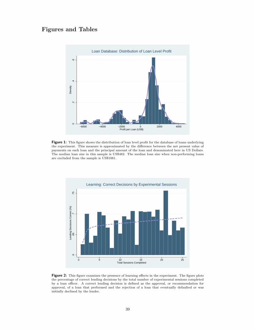
Figures and Tables

0.2

.4.6

Den

sity

0−6000 −2000 2000 4000−4000Profit per Loan (US$)

Loan Database: Distribution of Loan Level Profit

Figure 1: This figure shows the distribution of loan level profit for the database of loans underlyingthe experiment. This measure is approximated by the difference between the net present value ofpayments on each loan and the principal amount of the loan and denominated here in US Dollars.The median loan size in this sample is US$482. The median loan size when non-performing loansare excluded from the sample is US$1081.

.6.6

5.7

.75

Lend

ing

Dec

isio

ns C

orre

ct (

%)

0 5 10 15 20 25Total Sessions Completed

Learning: Correct Decisions by Experimental Sessions

Figure 2: This figure examines the presence of learning effects in the experiment. The figure plotsthe percentage of correct lending decisions by the total number of experimental sessions completedby a loan officer. A correct lending decision is defined as the approval, or recommendation forapproval, of a loan that performed and the rejection of a loan that eventually defaulted or wasinitially declined by the lender.

39

0.2

.4.6

.8K

erne

l Den

sity

4.5 5 5.5 6 6.5 7Log[Evaluation Time]

Baseline Supervisor Aligned Supervisor

Kernel Density: Evaluation Time

Figure 3: This figure plots the kernel density of log evaluation time by treatment. A Kolmogorov-Smirnov test for equality of distributions does not reject the equality of risk ratings under AlignedSupervisor Treatment and the Baseline, but rejects the equality of the Aligned Supervisor Treatmentand the Baseline Treatment at the 10% level.

0.0

1.0

2.0

3.0

4K

erne

l Den

sity

20 40 60 80 100Risk Rating, Performing Loans

Baseline Supervisor Aligned Supervisor

Risk Ratings: Performing Loans

Figure 4: This figure plots the kernel density of internal risk ratings for performing loans undereach experimental treatment. Kolmogorov-Smirnov tests for the equality of distributions rejects theequality of risk ratings under Supervisor Treatment and the Aligned Supervisor Treatment fromthe Baseline Treatment at the 5% level.

40

0.0

1.0

2.0

3.0

4K

erne

l Den

sity

20 40 60 80 100Risk Rating, Non−Performing Loans

Baseline Supervisor Aligned Supervisor

Risk Ratings: Non−Performing Loans

Figure 5: This figure plots the kernel density of internal risk ratings for non-performing loans undereach experimental treatment. Kolmogorov-Smirnov tests for the equality of distributions reject theequality of risk ratings under Supervisor Treatment and the Aligned Supervisor Treatment fromthe Baseline Treatment at the 1% level.

41

Figure 6: Loan Rating Exercise, Login

Figure 7: Loan Rating Exercise, Evaluation

42

Figure 8: Credit File, Sample

43

Table 1: Summary Statistics, Loan Officers

This table reports summary statistics for the pool of participants. Panel A summarizes the demographic characteristicsof the participants. Age is the loan officer’s age in years, Male is a dummy variable taking a value of 1 if the participantis male. Rank is the loan officer’s level seniority level in the bank. Experience is the total number of years the participanthas been employed with the bank. Branch Manager is a dummy indicating whether the participant has ever served asa branch manager. Panel B Evaluations reports on the participation and performance of the experimental subjects.Loans Evaluated is the number of unique loans evaluated by each participant over the course of his or her participationin the experiment. Loans approved is the share of affirmative lending decisions, Correct Decisions is the sum of LoansCorrectly approved and Loans Correctly Rejected, divided by the total number of lending decisions made by the loanofficer. Profit per session is the bank’s net profit of all loans made by the loan officer in an experimental session.

Panel A: Demographics

N Min Max Mean Median StdDev 10% 25% 75% 90%

Age 125 24 64 44.06 47.00 11.05 30.00 35.00 52.00 56.00

Male 125 0 1 0.95 1.00 0.21 1.00 1.00 1.00 1.00

Education [Master’s] 125 0 1 0.23 0.00 0.42 0.00 0.00 0.00 1.00

Experience [Years] 125 0 40 20.03 23.00 10.83 3.00 11.00 29.00 32.00

Rank [1 Low 5 High] 125 1 5 2.05 2.00 0.90 1.00 1.00 3.00 3.00

Branch Manager Experience [Yes/No] 125 0 1 0.49 0.00 0.50 0.00 0.00 1.00 1.00

Panel B: Evaluations

N Min Max Mean Median StdDev 10% 25% 75% 90%

Loans Evaluated 3,042 3 97 42 36 25.09 11 24 60 78

Loans Approved 3,042 0 1 0.72 1 0.45 0 0 1 1

Correct Decisions 3,042 0 1 0.66 1 0.47 0 0 1 1

Loans Correctly Approved 3,042 0 1 0.63 1 0.48 0 0 1 1

Loans Correctly Rejected 3,042 0 1 0.52 1 0.50 0 0 1 1

Profit per Loan Screened in US$ 3,042 -2429 1762 259 320 553 -478 -55 671 885

44

Table 2: Summary Statistics, Loans

This table reports summary statistics for the database of loans used in the experiment. Columns (1) to (3) showsummary statistics for the sub-sample of performing loans and columns (4) to (6) show summary statistics for thesub-sample of non-performing loans. Columns (7) and (8) show differences in means between the two groups andcorresponding standard errors. Principal Amount is the total principal amount of the loan, Monthly Installment is thegross monthly installment on the loan including the client’s payment towards principal and interest. Loan Tenure is theterm of the loan in months. Total Income is the client’s annual income from business and other sources before taxes andinterest expenses. Business Expenses measures the client’s annual business expenditure and includes current expensesand investments. EBIT are a client’s monthly earnings from business activities before taxes and interest. Total Debt isthe principal outstanding of all loans held by the client. Total Monthly Debt Service is the sum of the client’s EMIs onall outstanding loans. Liabilities/Net Income is the ratio of total liabilities, including interest expenses, to net annualincome. Liabilities/Sales is the ratio of total liabilities, including interest expenses, to net annual sales. EBIT/MonthlyDebt Service is the ratio of EBIT to the monthly loan installment, including payments towards principal and interest.

Panel A Panel B Panel CPerforming Loans Non-Performing Loans Difference in Means

Mean Median StdDev Mean Median StdDev Difference SEPrincipal Amount in US$ 5750.62 5364.81 2620.69 6456.59 6437.77 2718.48 705.97* [377.81]

Monthly Installment in US$ 194.09 168.28 89.73 163.29 149.27 83.39 -30.80** [13.78]

Loan Tenure [Months] 33.63 36.00 7.56 37.07 36.00 8.40 3.44** [1.643]

Years in Business 10.93 8.00 8.52 8.20 7.50 5.41 -2.73*** [0.994]

Total Income 11501.43 6437.77 15892.27 7160.23 4868.50 9812.86 -4341.43** [1781.04]

Total Debt in US$ 15730.58 1152.77 49349.21 7739.71 3387.64 12473.67 -7990.86** [3434.88]

Monthly Debt Service 374.95 62.27 1097.05 273.37 120.17 407.34 -101.58 [85.03]

EBIT 1899.98 1019.31 3872.11 1430.58 1105.15 1050.06 -469.40* [281.21]

Business Expenditure 9676.99 5386.27 14206.70 5704.47 3862.66 9004.86 -3972.51*** [1621.59]

Liabilities/Net Income 0.04 0.02 0.10 0.06 0.03 0.07 0.02* [0.013]

Liabilities/Sales 0.034 0.016 0.051 0.060 0.032 0.070 0.024** [0.011]

EBIT/Monthly Debt Service 7.19 3.811 26.70 4.69 2.24 3.98 -2.54** [4.122]

45

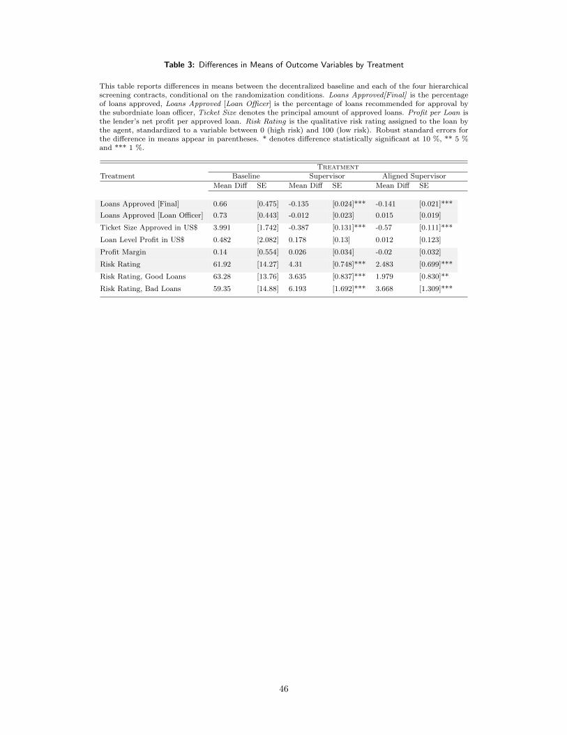
Table 3: Differences in Means of Outcome Variables by Treatment

This table reports differences in means between the decentralized baseline and each of the four hierarchicalscreening contracts, conditional on the randomization conditions. Loans Approved[Final] is the percentageof loans approved, Loans Approved [Loan Officer] is the percentage of loans recommended for approval bythe subordniate loan officer, Ticket Size denotes the principal amount of approved loans. Profit per Loan isthe lender’s net profit per approved loan. Risk Rating is the qualitative risk rating assigned to the loan bythe agent, standardized to a variable between 0 (high risk) and 100 (low risk). Robust standard errors forthe difference in means appear in parentheses. * denotes difference statistically significant at 10 %, ** 5 %and *** 1 %.

TreatmentTreatment Baseline Supervisor Aligned Supervisor

Mean Diff SE Mean Diff SE Mean Diff SE

Loans Approved [Final] 0.66 [0.475] -0.135 [0.024]*** -0.141 [0.021]***

Loans Approved [Loan Officer] 0.73 [0.443] -0.012 [0.023] 0.015 [0.019]

Ticket Size Approved in US$ 3.991 [1.742] -0.387 [0.131]*** -0.57 [0.111]***

Loan Level Profit in US$ 0.482 [2.082] 0.178 [0.13] 0.012 [0.123]

Profit Margin 0.14 [0.554] 0.026 [0.034] -0.02 [0.032]

Risk Rating 61.92 [14.27] 4.31 [0.748]*** 2.483 [0.699]***

Risk Rating, Good Loans 63.28 [13.76] 3.635 [0.837]*** 1.979 [0.830]**

Risk Rating, Bad Loans 59.35 [14.88] 6.193 [1.692]*** 3.668 [1.309]***

46

Table 4: Treatment Effects: Effort

This table shows treatment effects on the screening effort measured as the total time spent reviewing a loan file andthe number of information credits spent to review individual sections of the loan file. The omitted category in eachregression is the non-supervised baseline treatment. The dependent variable in all equations is the log of the loanofficer’s total evaluation time per credit file. In addition to the variables listed, I control for the five randomizationstrata from which assigned treatments were drawn, an indicator for the experimental lab, and the ticket size of the loanin all specifications that do not include loan fixed effects. Standard errors are clustered at the individual and sessionlevel. * denotes statistical significance at 10 %, ** 5 % and *** 1 %.

Dependent Variable Log[Time] Log[Time] Log[Time] Log[Time]OLS OLS OLS OLS

(1) (2) (3) (4)

Baseline [Non-Supervised]

Supervisor -0.023 -0.060 -0.081 -0.068[0.043] [0.035]* [0.038]** [0.040]*

Aligned Supervisor 0.094 0.093 0.092 0.060[0.051]* [0.036]*** [0.036]** [0.034]*

F-Test, Supervisor+Aligned=0 1.97 0.70 0.07 0.03P-Value [0.167] [0.403] [0.798] [0.852]Loan Officer Fixed Effects No Yes Yes YesSupervisor Fixed Effects No Yes Yes YesWeek Fixed Effects No No Yes YesLoan Fixed Effects No No No Yes

Number of Observations 2,097 2,097 2,097 2,158R-Squared 0.099 0.480 0.581 0.652

47

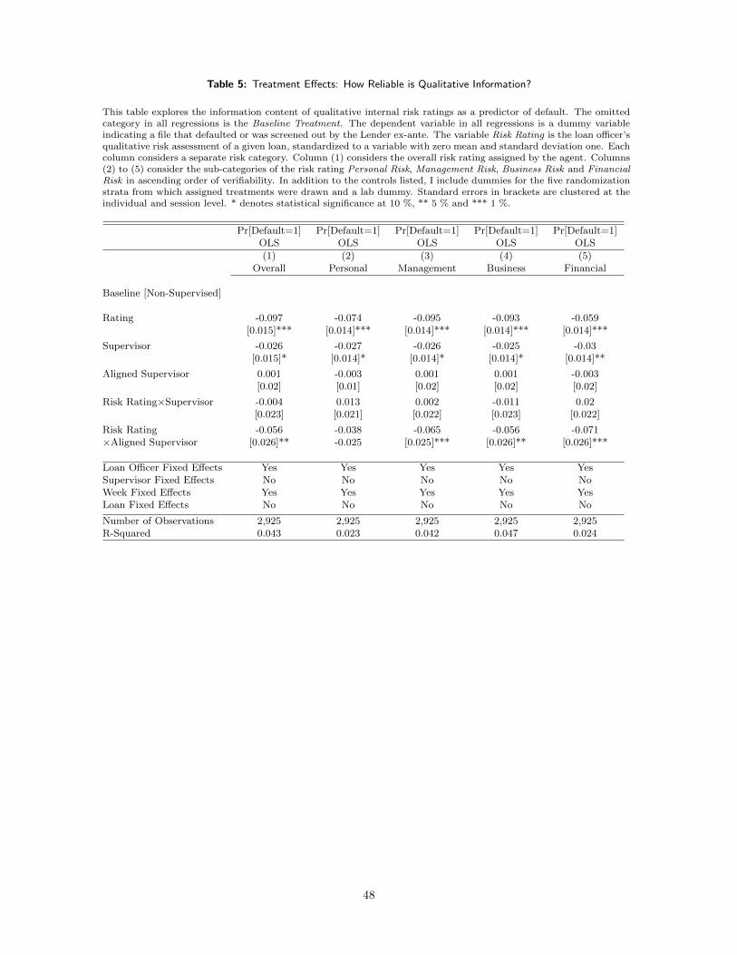
Table 5: Treatment Effects: How Reliable is Qualitative Information?

This table explores the information content of qualitative internal risk ratings as a predictor of default. The omittedcategory in all regressions is the Baseline Treatment. The dependent variable in all regressions is a dummy variableindicating a file that defaulted or was screened out by the Lender ex-ante. The variable Risk Rating is the loan officer’squalitative risk assessment of a given loan, standardized to a variable with zero mean and standard deviation one. Eachcolumn considers a separate risk category. Column (1) considers the overall risk rating assigned by the agent. Columns(2) to (5) consider the sub-categories of the risk rating Personal Risk, Management Risk, Business Risk and FinancialRisk in ascending order of verifiability. In addition to the controls listed, I include dummies for the five randomizationstrata from which assigned treatments were drawn and a lab dummy. Standard errors in brackets are clustered at theindividual and session level. * denotes statistical significance at 10 %, ** 5 % and *** 1 %.

Pr[Default=1] Pr[Default=1] Pr[Default=1] Pr[Default=1] Pr[Default=1]OLS OLS OLS OLS OLS

(1) (2) (3) (4) (5)Overall Personal Management Business Financial

Baseline [Non-Supervised]

Rating -0.097 -0.074 -0.095 -0.093 -0.059[0.015]*** [0.014]*** [0.014]*** [0.014]*** [0.014]***

Supervisor -0.026 -0.027 -0.026 -0.025 -0.03[0.015]* [0.014]* [0.014]* [0.014]* [0.014]**

Aligned Supervisor 0.001 -0.003 0.001 0.001 -0.003[0.02] [0.01] [0.02] [0.02] [0.02]

Risk Rating×Supervisor -0.004 0.013 0.002 -0.011 0.02[0.023] [0.021] [0.022] [0.023] [0.022]

Risk Rating -0.056 -0.038 -0.065 -0.056 -0.071×Aligned Supervisor [0.026]** -0.025 [0.025]*** [0.026]** [0.026]***

Loan Officer Fixed Effects Yes Yes Yes Yes YesSupervisor Fixed Effects No No No No NoWeek Fixed Effects Yes Yes Yes Yes YesLoan Fixed Effects No No No No No

Number of Observations 2,925 2,925 2,925 2,925 2,925R-Squared 0.043 0.023 0.042 0.047 0.024

48

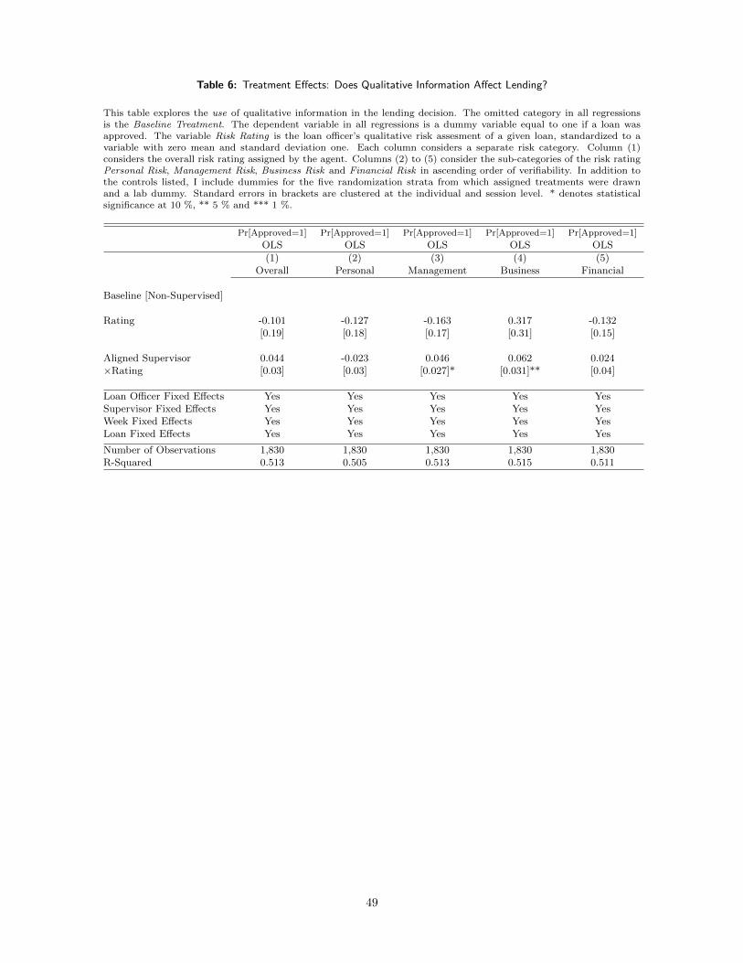
Table 6: Treatment Effects: Does Qualitative Information Affect Lending?

This table explores the use of qualitative information in the lending decision. The omitted category in all regressionsis the Baseline Treatment. The dependent variable in all regressions is a dummy variable equal to one if a loan wasapproved. The variable Risk Rating is the loan officer’s qualitative risk assesment of a given loan, standardized to avariable with zero mean and standard deviation one. Each column considers a separate risk category. Column (1)considers the overall risk rating assigned by the agent. Columns (2) to (5) consider the sub-categories of the risk ratingPersonal Risk, Management Risk, Business Risk and Financial Risk in ascending order of verifiability. In addition tothe controls listed, I include dummies for the five randomization strata from which assigned treatments were drawnand a lab dummy. Standard errors in brackets are clustered at the individual and session level. * denotes statisticalsignificance at 10 %, ** 5 % and *** 1 %.

Pr[Approved=1] Pr[Approved=1] Pr[Approved=1] Pr[Approved=1] Pr[Approved=1]

OLS OLS OLS OLS OLS

(1) (2) (3) (4) (5)Overall Personal Management Business Financial

Baseline [Non-Supervised]

Rating -0.101 -0.127 -0.163 0.317 -0.132[0.19] [0.18] [0.17] [0.31] [0.15]

Aligned Supervisor 0.044 -0.023 0.046 0.062 0.024×Rating [0.03] [0.03] [0.027]* [0.031]** [0.04]

Loan Officer Fixed Effects Yes Yes Yes Yes YesSupervisor Fixed Effects Yes Yes Yes Yes YesWeek Fixed Effects Yes Yes Yes Yes YesLoan Fixed Effects Yes Yes Yes Yes Yes

Number of Observations 1,830 1,830 1,830 1,830 1,830R-Squared 0.513 0.505 0.513 0.515 0.511

49

Table 7: Treatment Effects: Lending Decisions

This table shows treatment effects on lending decisions. The omitted category in each regression is the non-supervisedbaseline treatment. In column (1), the dependent variable is a dummy indicating whether a loan was approved (es-calated) by the agent. In column (2) the dependent variable is a dummy indicating whether a loan was approved bythe principal. In column (3) the dependent variable is a dummy indicating the final lending decision. The dependentvariable in column (4) is the principal amount approved, denominated in US$ 1000 and equal to zero if a loan wasdeclined. In column (5) the dependent variable is the loan amount approved, denominated in units of US$ 1000 andthe sample is restricted to approved loans. In addition to the variables listed, I control for the five randomization stratafrom which assigned treatments were drawn and an indicator for the experimental lab. Standard errors are clusteredat the individual and session level. * denotes statistical significance at 10 %, ** 5 % and *** 1 %.

Dependent Variable Agent Principal Final Decision Lending Volume Ticket SizePr[Approve=1] Pr[Approve=1] Pr[Approve=1] USD[’000] USD[’000]

OLS OLS OLS OLS OLS

(1) (2) (3) (4) (5)

Baseline [Non-Supervised]

Supervisor 0.071 -0.158 -0.067 -0.235 -0.516[0.036]** [0.028]*** [0.036]* [0.181] [0.120]***

Aligned Supervisor 0.014 0.020 0.031 0.271 0.193[0.031] [0.029] [0.030] [0.152]* [0.134]

Loan Officer Fixed Effects Yes Yes Yes Yes YesSupervisor Fixed Effects No Yes Yes Yes YesWeek Fixed Effects Yes Yes Yes Yes YesLoan Fixed Effects Yes Yes Yes Yes Yes

Number of Observations 2,517 1,830 2,517 2,108 1,644R-Squared 0.368 0.480 0.409 0.543 0.771

50

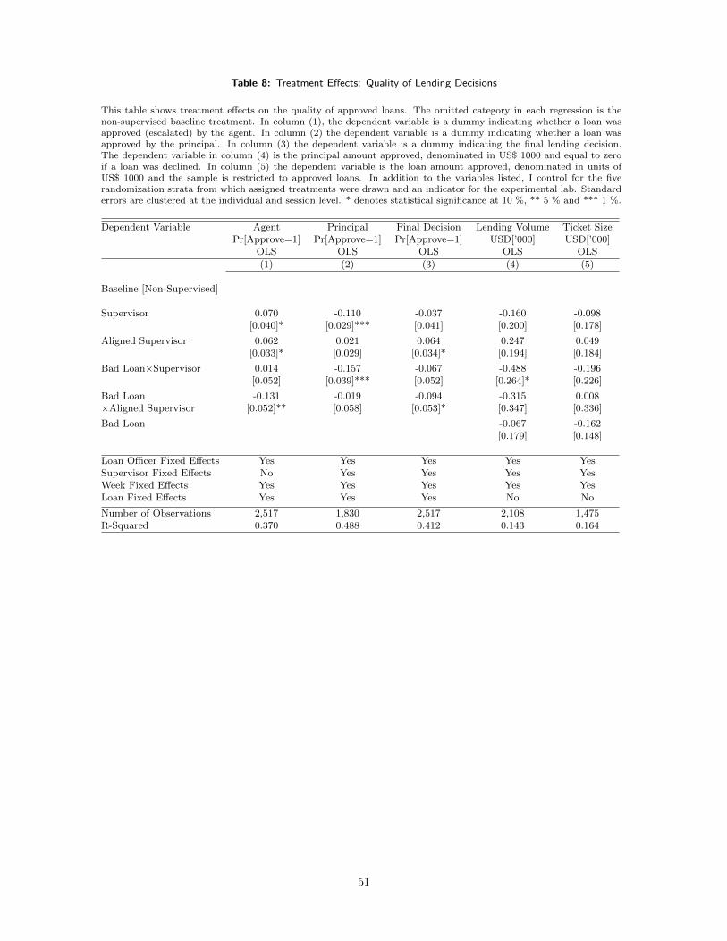
Table 8: Treatment Effects: Quality of Lending Decisions

This table shows treatment effects on the quality of approved loans. The omitted category in each regression is thenon-supervised baseline treatment. In column (1), the dependent variable is a dummy indicating whether a loan wasapproved (escalated) by the agent. In column (2) the dependent variable is a dummy indicating whether a loan wasapproved by the principal. In column (3) the dependent variable is a dummy indicating the final lending decision.The dependent variable in column (4) is the principal amount approved, denominated in US$ 1000 and equal to zeroif a loan was declined. In column (5) the dependent variable is the loan amount approved, denominated in units ofUS$ 1000 and the sample is restricted to approved loans. In addition to the variables listed, I control for the fiverandomization strata from which assigned treatments were drawn and an indicator for the experimental lab. Standarderrors are clustered at the individual and session level. * denotes statistical significance at 10 %, ** 5 % and *** 1 %.

Dependent Variable Agent Principal Final Decision Lending Volume Ticket SizePr[Approve=1] Pr[Approve=1] Pr[Approve=1] USD[’000] USD[’000]

OLS OLS OLS OLS OLS

(1) (2) (3) (4) (5)

Baseline [Non-Supervised]

Supervisor 0.070 -0.110 -0.037 -0.160 -0.098[0.040]* [0.029]*** [0.041] [0.200] [0.178]

Aligned Supervisor 0.062 0.021 0.064 0.247 0.049[0.033]* [0.029] [0.034]* [0.194] [0.184]

Bad Loan×Supervisor 0.014 -0.157 -0.067 -0.488 -0.196[0.052] [0.039]*** [0.052] [0.264]* [0.226]

Bad Loan -0.131 -0.019 -0.094 -0.315 0.008×Aligned Supervisor [0.052]** [0.058] [0.053]* [0.347] [0.336]

Bad Loan -0.067 -0.162[0.179] [0.148]

Loan Officer Fixed Effects Yes Yes Yes Yes YesSupervisor Fixed Effects No Yes Yes Yes YesWeek Fixed Effects Yes Yes Yes Yes YesLoan Fixed Effects Yes Yes Yes No No

Number of Observations 2,517 1,830 2,517 2,108 1,475R-Squared 0.370 0.488 0.412 0.143 0.164

51

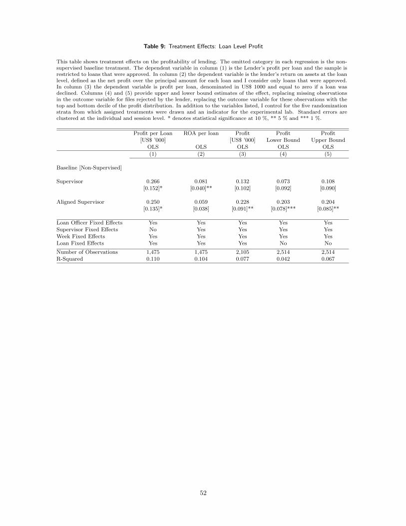
Table 9: Treatment Effects: Loan Level Profit

This table shows treatment effects on the profitability of lending. The omitted category in each regression is the non-supervised baseline treatment. The dependent variable in column (1) is the Lender’s profit per loan and the sample isrestricted to loans that were approved. In column (2) the dependent variable is the lender’s return on assets at the loanlevel, defined as the net profit over the principal amount for each loan and I consider only loans that were approved.In column (3) the dependent variable is profit per loan, denominated in US$ 1000 and equal to zero if a loan wasdeclined. Columns (4) and (5) provide upper and lower bound estimates of the effect, replacing missing observationsin the outcome variable for files rejected by the lender, replacing the outcome variable for these observations with thetop and bottom decile of the profit distribution. In addition to the variables listed, I control for the five randomizationstrata from which assigned treatments were drawn and an indicator for the experimental lab. Standard errors areclustered at the individual and session level. * denotes statistical significance at 10 %, ** 5 % and *** 1 %.

Profit per Loan ROA per loan Profit Profit Profit[US$ ’000] [US$ ’000] Lower Bound Upper Bound

OLS OLS OLS OLS OLS

(1) (2) (3) (4) (5)

Baseline [Non-Supervised]

Supervisor 0.266 0.081 0.132 0.073 0.108[0.152]* [0.040]** [0.102] [0.092] [0.090]

Aligned Supervisor 0.250 0.059 0.228 0.203 0.204[0.135]* [0.038] [0.091]** [0.078]*** [0.085]**

Loan Officer Fixed Effects Yes Yes Yes Yes YesSupervisor Fixed Effects No Yes Yes Yes YesWeek Fixed Effects Yes Yes Yes Yes YesLoan Fixed Effects Yes Yes Yes No No

Number of Observations 1,475 1,475 2,105 2,514 2,514R-Squared 0.110 0.104 0.077 0.042 0.067

52

Appendix Tables

Table A1: Test of Random Assignment

This table provides a test of random assignment. The table shows the mans of observable pre-treatment character-istics for the population of paerticipating loan officers for the baseline and each treatment. Reported p-values (inbrackets) correspond to a test for a difference in means between the baseline and each treatment and are obtainedfrom least squares regressions, controlling for treatment condition and an indicator variable for the experimentallab at which the experiment was carried out. Standard errors are clustered at the loan officer level. * indicates adifference in means significant at the 10 %, ** 5 % and *** 1 % level.

TreatmentBaseline Supervisor Supervisor

(N=1,629) Basic (N=786) Aligned (N=627)

Mean SE Mean p > |t| Mean p > |t|

Male 0.94 [0.006] 0.961 [0.294] 0.901 [0.380]

Age 46.18 [0.289] 42.73 [0.242] 43.15 [0.854]

Education [Master’s Degree] 0.31 [0.013] 0.291 [0.863] 0.328 [0.566]

Experience in Bank [Years] 21.30 [0.296] 18.54 [0.189] 18.58 [0.238]

Rank [1-5] 2.02 [0.026] 2.13 [0.104] 2.03 [0.285]

Branch Manager Experience 0.56 [0.014] 0.488 [0.990] 0.443 [0.669]

Business Experience 0.69 [0.013] 0.627 [0.275] 0.610 [0.145]

Table A2: Participation

This table reports participation rates in the experiment. The first column shows the total number of loanofficers contacted by bank, the second column shows the percentage of loan officers who participated in theexperiment. Columns (3) and (4) summarize the average rank and years of experience of the participatingloan officers by bank.

Invited Participated (%) Mean Rank (1-5) Mean Experience (Years)

Bank of Baroda 127 0.69 2.25 13.71

State Bank of India 76 0.39 2.06 14.77

Punjab National Bank 31 0.35 2.00 23.93

Bank of India 11 0.82 2.22 30.84

Other Banks 10 0.70 2.00 18.25

53

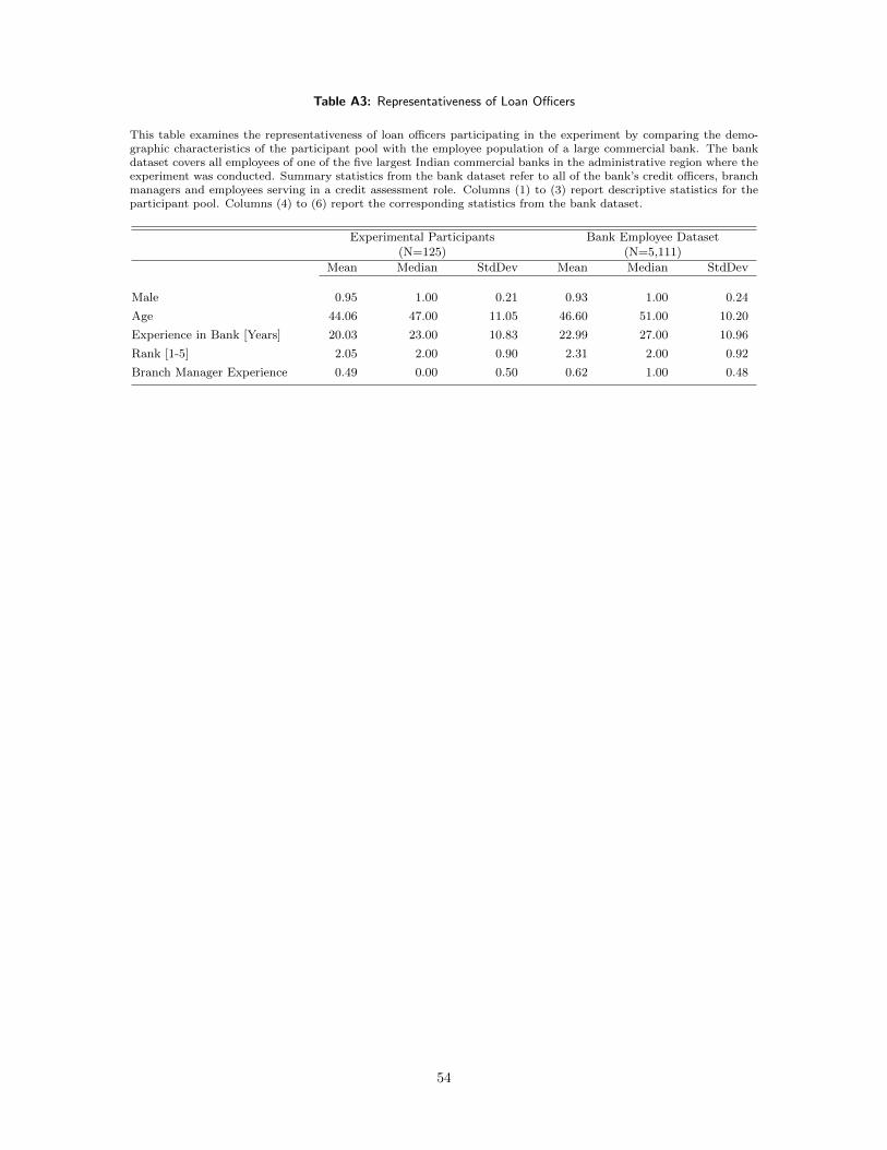
Table A3: Representativeness of Loan Officers

This table examines the representativeness of loan officers participating in the experiment by comparing the demo-graphic characteristics of the participant pool with the employee population of a large commercial bank. The bankdataset covers all employees of one of the five largest Indian commercial banks in the administrative region where theexperiment was conducted. Summary statistics from the bank dataset refer to all of the bank’s credit officers, branchmanagers and employees serving in a credit assessment role. Columns (1) to (3) report descriptive statistics for theparticipant pool. Columns (4) to (6) report the corresponding statistics from the bank dataset.

Experimental Participants Bank Employee Dataset(N=125) (N=5,111)

Mean Median StdDev Mean Median StdDev

Male 0.95 1.00 0.21 0.93 1.00 0.24

Age 44.06 47.00 11.05 46.60 51.00 10.20

Experience in Bank [Years] 20.03 23.00 10.83 22.99 27.00 10.96

Rank [1-5] 2.05 2.00 0.90 2.31 2.00 0.92

Branch Manager Experience 0.49 0.00 0.50 0.62 1.00 0.48

54