Bargaining, Mergers, and Heterogeneous

Outsiders∗

Malte Cherdron† Konrad Stahl‡

September 24, 2001

Abstract

We extend the cooperative analysis of bargaining and mergers in Se-gal (2000) by allowing for outsider heterogeneity. In real-life industrieswith bilateral bargaining, firms commonly face very different trading part-ners. For instance, the upstream suppliers and downstream customersof intermediate-input producers are likely to differ fundamentally in theirbargaining positions. We show that heterogeneity leads to interesting im-plications of mergers even in a pure bargaining model with fixed totalsurplus: Outsiders can be the main beneficiaries of a profitable merger,and shocks to outsiders can be more than compensated by a subsequentmerger decision. Moreover, a richer set of outsiders turns independentmerger decisions into strategic complements or substitutes, leading to abargaining-based rationale for merger and de-merger “waves”.

Keywords: Bargaining, Shapley value, mergers, heterogeneity, mergerwaves, strategic complements.

Filename: bargaining-01.tex (1330)

∗We would like to thank Martin Hellwig for his comments on an earlier version of this paper.Financial support from the Deutsche Forschungsgemeinschaft is gratefully acknowledged.

†CDSEM, Department of Economics, Universitat Mannheim, D-68131 Mannheim, Germany.E-mail: cherdron@econ.uni-mannheim.de

‡Universitat Mannheim, CEPR, CESifo, and ZEW. E-mail: konrad@econ.uni-mannheim.de

1

1 Introduction

Despite the prevelance in economic theory of markets with many players on one

or both sides, trade in real life very often takes place on a bilateral basis with a

single buyer and seller bargaining over the terms of trade. This is particularly

true for intermediate goods traded within the kind of multi-tiered, oligopolistic

market structure often referred to as an “industry”. Of particular interest in such

a setting is the relationship between market structure and bargaining outcomes.

This is more than just a theoretical exercise. Over the past two decades,

mergers and acquisitions have played a very prominent role in the evolution of

many important industries.1 DaimlerChrysler, AOL Time Warner and Novartis

are just three of the most well-known examples; others like the GE-Honeywell

merger failed to become reality only because of exogenous obstacles. Somewhat

less spectacular but nonetheless important for their industries, there have been

a number of de-mergers like the spin-off of Delphi from General Motors. Yet the

economic theory of mergers remains very incomplete. The explanations of merger

incentives range from monopolization motives to “synergies” and empire-building

by ill-controlled managers. Another aspect which has attracted some attention

is the impact of a merger on bargaining shares.2 However, not very much is

known about the bargaining effects of mergers in multi-tiered industries with

heterogeneous firms; nor is there yet a fully convincing theoretical explanation of

merger waves.

This paper is a contribution towards the development of a more general theory

of bargaining and mergers in industries with bilateral trade among very differ-

ent players. We build on the cooperative approach recently developed by Segal

(2000), paying particular attention to the role of heterogeneity among the out-

siders to a given merger. Abstracting from allocative effects and concentrating

on bargaining considerations alone, we find that heterogeneity among outsiders

gives rise to a number of new effects: Outsiders can be the main beneficiaries

of a profitable merger; the final consequences of player-specific shocks can be

quite different from the initial effect; and the merger decisions of two disjoint

pairs of firms are generally strategic complements or substitutes, suggesting a

bargaining-based rationale for mergers to occur in waves.

Throughout, we take the candidate players for a merger as exogenously given.

1See, for instance, Gugler et al. (2001).2Segal (2000) gives an overview of the literature on integration and bargaining.

2

In this assumption, and in the flavour of some of our results, this paper is related

to the exogenous-mergers literature following Stigler (1950), which focuses on

mergers among homogeneous firms in a single market. A standard reference is

the paper by Salant et al. (1983), who famously show that the merging firms in

a Cournot oligopoly with constant marginal cost must have a market share of

at least 80% in order for the merger to be profitable. Heuristically, the merging

firms move the industry allocation closer to the cartel outcome (by internalizing

the external effects they exert on each other) but lose some market power by

becoming a single player instead of several independent ones; the net effect is

ambiguous for the merging firms but positive for all outsiders. More recently,

Nilssen and Sørgard (1998) have extended this approach to study the interaction

between disjoint mergers within the framework of Fudenberg and Tirole (1984).

However, the combination of allocative and market-power effects, as well as the

marginal-cost synergies assumed by Nilssen and Sørgard, make it difficult to

consider each effect in isolation even in a simple, horizontal market.

In a related strand of the literature, the interaction of upstream and down-

stream players is taken into consideration in the analysis of merger incentives

within a non-cooperative framework. Examples include the application to union

formation in Horn and Wolinsky (1988b) and Stole and Zwiebel (1996b); Stole

and Zwiebel (1998); and most recently the supplier–retailer model of Inderst and

Wey (2001). A notable improvement of the last paper over some predecessors

like Horn and Wolinsky (1988a) lies in the use of “efficient” bargaining (i. e. over

quantities as well as prices), which eliminates any allocative effects of a merger

and allows for an analysis based entirely on bargaining-power considerations.

Broadly speaking, a merger in this setting—like in Horn and Wolinsky (1988b)—

is profitable if the merging players face a common supplier operating at increasing

unit cost, or a common customer who regards their output as substitutable. In

either case, a merger shifts the focus of each bilateral bargaining session towards

the higher inframarginal rents, resulting in an increased payoff for the merged

entity.

Segal (2000) takes the analysis of mergers (“collusion”, in his terms) to an-

other level using a cooperative approach in which the joint profit of any coalition

of firms is always maximized by definition, and where the game is entirely about

the distribution of rents.3 In contrast with the very specific, non-cooperative

3Inderst and Wey (2001) obtain an equivalent setting by a combination of efficient bargainingand assumptions ruling out coordination failures.

3

models in the earlier literature, Segal’s approach leads to a unifying view of the

underlying bargaining effects in a very general setting. Among other things, he

shows that the profitability of a merger is determined by the impact of the outside

players on the substitutability of the merging firms rather than the level of that

substitutabilty per se.

A limitation of almost all previous work, however, lies in the way outsiders

are modeled. Since the focus is generally on merger incentives as such, relatively

little attention is paid to outsiders’ characteristics. To simplify matters, they

are usually taken to be essentially homogeneous. For instance, while the basic

model in Inderst and Wey (2001) allows for heterogeneity, no attention is given

to the case where one supplier has increasing unit costs while the other operates

under economies of scale. Segal (2000) employs a robustness condition with

respect to the choice of random-order values which implies that all outsiders

must either increase or decrease the merging players’ substitutability, ruling out

the interesting case where there are both types of outsiders.

While we follow Segal’s very general cooperative approach, we concentrate on

the effects of a merger on heterogeneous outsiders, restricting our attention to

Shapley values rather than general random-order values. Relative to Segal, this

implies that we take intrinsic bargaining abilities as known ex ante. Regardless of

this restriction, individual payoffs depend on the marginal contributions of each

player to various preceding coalitions; heuristically, these correspond to different

bargaining situations where some of the other players refuse to cooperate.

Mergers or de-mergers in our model affect payoffs by changing the composi-

tion of the preceding coalitions in each ordering of the players. Intuitively, this

corresponds to a change in the set of different bargaining situations in which each

player finds himself after some of the other have refused to cooperate. A recurring

theme will be the complementarity of two merging players in the presence of some

outsiders. When two players have merged, they employ or withdraw their joint

resources together rather than separately. This has an impact on the average

marginal contributions of the other players because it replaces each bargaining

situation where only one of the merging parties is active by one in which either

both or neither of them participate. If the merging parties are complementary in

their impact on the remaining players, then their joint impact exceeds the sum

of their individual effects. We make this argument more precise below using a

second-difference operator introduced by Segal (2000) (and earlier, by Ichiishi

(1993)) to capture the complementarity of the merging players.

4

A key feature of our analysis is that we allow outsiders to be heterogeneous.

In real life, bargaining takes place in fairly complex settings, where the players

can face very different bilateral-trading partners at the same time. For example,

producers of intermediate inputs deal with both downstream customers and up-

stream suppliers, and there is no reason to assume that these two kinds of trading

partners share any fundamental characteristics. The same is true in the case of a

vertical merger. Even the outsiders to a horizontal merger in a simple two-sided

market can very easily be fundamentally different. For example, there is nothing

exceptional about a firm dealing simultaneously with some suppliers producing

at increasing unit cost, and with others enjoying economies of scale.

The automobile industry is a case in point. Intermediate-input suppliers of au-

tomobile producers are loosely organized into so-called tiers. Tier 0 encompasses

the automotive producers; tier 1 their parts and components suppliers; and tier 2

the suppliers of materials and parts to the latter. Depending on their degree of

vertical integration and/or their product portfolio, some car makers may con-

sider particular bundles of intermediate inputs as substitutes, while others may

consider them as complements. Tier-1 suppliers producing diverse intermediate

inputs can vary fundamentally in their marginal contributions to various coali-

tions of firms in the industry. Their tier-2 suppliers in turn range from small

firms providing specialized springs exclusively to the industry at increasing aver-

age costs, to large steel producers supplying raw metal sheets to many industries

at strongly decreasing average costs. In addition, on their output side, car makers

might also be dealing with different retailing channels. For instance, car brands

or model types might be substitutes in small local markets but complements for

a large-scale retailer trying to expand its geographical reach.

Outsider heterogeneity is not only an important empirical phenomenon; it

also leads to effects which are otherwise absent in pure bargaining models. If all

outsiders are fundamentally alike, then a merger in a zero-sum game can only be

profitable if it hurts all outsiders. It follows immediately that the heterogeneity

of outsiders is a necessary condition for some of them to benefit from a profitable

merger. Indeed, when outsiders differ sufficiently, then the main effect of a merger

can be a redistribution of surplus from some outsiders to others, while the merging

firms themselves receive only a small share of the redistributed rents.

This is of particular interest when an outsider is hit by an exogenous shock

prior to the merger decision. Even a shock specific to that outsider can have

an indirect effect, in addition to the obvious direct one. This is because the

5

characteristics of the affected outsider have an influence on the contributions of

other players and, therefore, on how they are affected by a merger. By changing

the amount of surplus received by each outsider after a merger, the shock can

change the merger decision itself, which in turn can more than compensate the

payoff effect of the shock originally experienced by the affected outsider.

This has important implications for empirical studies. First of all, the corre-

lation between firm-specific shocks and profits is distorted or even reversed when

these shocks result in mergers (or de-mergers) in the same industry. (Note that

an “industry” in our context includes all the firms which are part of the same

buyer-supplier network, so the merger need not occur in the immediate vicinity

of the firm affected by the shock.) Second, the main incidence of the shock may

fall on players who are only indirectly connected to the one originally affected.

Re-interpreting the exogenous shock as the (binding) technology adoption of an

outsider, we also conclude that the prospect of a merger can lead to inefficient

incentives for technology choice and R&D effort.

The existence of different kinds of outsiders is also a necessary and generically

sufficient condition for the interaction of two disjoint mergers. When there are

additional outsiders who do not take part in either merger, then the two merg-

ers interact symmetrically, turning merger decisions into strategic substitutes or

complements. This qualifies an intermediate result derived by Inderst and Wey

(2001), who find that the merger decisions of two disjoint pairs of players are

independent of each other in a four-firm industry. Our results show that this

does not generalize to a setting with more than four firms because each merger

affects the impact of the other on the payoffs of those players who participate in

neither.

The remainder of this paper is organized as follows. We motivate our use

of a cooperative model in Appendix A, where we show that the Shapley value

is a useful solution concept in a very general setting of bilateral bargaining if

one abstracts from allocative externalities and coordination problems to con-

centrate exclusively on bargaining effects.4 In spite of some limitations of our

non-cooperative foundation (for instance, there is no extensive form for the simul-

taneous bilateral negotiations), we take this as an argument for following and ex-

tending Segal’s general cooperative approach as against specific non-cooperative

models which are subject to similar limitations without offering the same gener-

4In contrast with Inderst and Wey (2001), we motivate the Shapley value by a stabilityconcept generalized from Stole and Zwiebel (1996), rather than by contingent contracts.

6

ality of results.

The basic model is introduced in the next section, along with a measure of

merger effects based on the Shapley value. Our notion of heterogeneity is defined

in Section 3 and shown to be necessary for outsiders to benefit from a profitable

merger. Section 4 contains the analysis of an exogenous shock experienced by

one of the outsiders before the merger decision. In Section 5 we consider the

interaction between two mergers. Section 6 concludes. Our main results are

illustrated in two examples in Sections 4.1 and 5.4. Some proofs are contained in

Appendix B.

2 The Model

Consider a cooperative game with transferable utility among a set of players

N = {1, . . . , n}. For instance, N can be thought of as an industry consisting of n

firms facing each other in various vertical and horizontal bilateral relationships.

As usual, the characteristic function v : 2N → R+ defines the worth of any

coalition S ⊆ N . This is the maximum total net profit which the members of

S can achieve collectively if they coordinate their actions in the absence of the

remaining players N \ S. The worth of the empty set is normalized to zero,

v(∅) = 0. Note that v(S) depends only on the resources available to the players

in S; the allocation of control rights over those resources affects individual payoffs

but not the overall worth of the coalition S.

A merger of two players a and b in N is the binding decision to face all

other players as a single entity which simultaneously contributes (or withdraws)

the joint resources of its constituent parts in any given bargaining situation.

Likewise, a de-merger is the decision to separate an entity into two independent

players each of whom controls some of the joint resources. We assume that there

is at most one technologically feasible way of partitioning the resources of any

player into two independent units. Moreover, neither a merger nor a demerger

affects the joint contribution of both players to any given coalition in N ; that is,

we explicitly rule out synergies and diseconomies of scale.

At some points we will assume that v(S) is a continuous function of a param-

eter λ. What we have in mind is a parameter with a continuous effect on the

underlying profit functions of one or several of the players in N and, hence, on

the optimal joint payoff which any given coalition S can achieve. For example, λ

might represent the marginal cost of a supplier or the number of final consumers.

7

The game is solved by the Shapley (1953) value. Let Π denote the set of all

n! permutations of the n players, and let π ∈ Π denote a particular permutation

(or ordering). Further, let

∆i(S) ≡ v(S ∪ i)− v(S)

denote the marginal contribution of player i /∈ S to coalition S ⊂ N .5 As is well

known, the Shapley value is derived axiomatically and prescribes that each player

receive his average marginal contribution to the coalition of players preceding him

in each ordering π ∈ Π, with the same probability weight of 1/n! accorded to

each ordering.

Let ≺π denote precedence in ordering π, so that

{a, b} ≺π {c, d}

if and only if players a and b precede players c and d in ordering π, regardless of

the pairwise ordering of a and b, and c and d respectively. Let

B(i, π) ≡ {k ∈ N : k ≺π i}

denote the set of players preceding player i in ordering π. In other words, B(i, π)

is the coalition of players to which i makes his marginal contribution in this

ordering.

The Shapley value for player i is given by

Shi =1

n!

∑π∈Π

∆i(B(i, π)).

Non-cooperative foundations for the Shapley value have been given by Gul

(1989), Hart and Mas-Colell (1996), and Stole and Zwiebel (1996a) among others.

To motivate our use of the Shapley value, Appendix A contains a generalization

of the stability condition developed by Stole and Zwiebel (1996a). At the core

of this concept is the assumption that renegotiation is always possible. Thus,

disagreement payoffs in any bilateral bargaining situation are given by what the

players can achieve after a general renegotiation of all active contracts rather than

by what is specified in the equilibrium set of contracts.6 We present a setup where

5For simplicity, we denote the single-element set {i} as i. The difference-operator notation isborrowed and adapted from Segal (2000), who credits Ichiishi (1993) with an earlier introductionof the same concept to describe complementarities between players in cooperative games.

6Inderst and Wey (2001) achieve the same result by letting firm bargain over sets of contractscontingent on the outcomes of all other bilateral negotiations.

8

the firms in an industry are connected through a set of bilateral trading links.

The terms of trade are also determined bilaterally by delegated, simultaneous,

and efficient bargaining. Stole–Zwiebel stability in this setup implies that payoffs

obey Myerson’s (1980) “fair allocation” rule, and hence, by his central result, are

equal to the players’ Shapley values.

2.1 A measure of merger effects

This section is based largely on Segal (2000), who analyzes mergers as a combina-

tion of exclusive and inclusive contracts, arriving at essentially the same measure

of merger effects (4) in a closely related way.7

The impact Mk(ab) of a merger of any two firms a, b in N on an outsider

k ∈ N \ {a, b} is the difference between her Shapley values after and before the

merger,

Mk(ab) ≡ Shk∣∣a and b merged

− Shk∣∣a and b separate

,

where the Shapley value after the merger of a and b is evaluated over all per-

mutations of the remaining n− 1 players; one of these is the merged firm whose

marginal contribution to a preceding coalition B is the sum of the contributions

of its components a and b, ∆a(B)+∆b(B ∪ a). To determine Mk(ab), it is useful

to introduce the notion of a dummy player.

Definition 1 A player i ∈ N is called a dummy player if and only if v(S ∪ i) =v(S \ i) for all S ⊆ N .

Using this definition, we can evaluate post-merger Shapley values over the per-

mutations of the original n players, which allows us to compare the effect of the

merger for each permutation.

It is easily checked that adding a single dummy player to the set of n−1 post-

merger players has no effect on the Shapley values of the n−1 “real” players. Let

Nm denote the set of players consisting of the merged firm, the n− 2 outsiders in

N \ {a, b}, and the dummy player. Let Πm be the set of n! permutations of the

players in Nm. The post-merger payoff to an outsider k ∈ N \ {a, b} is equal to

Shk∣∣a and b merged

=1

n!

∑πm∈Πm

∆k(B(k, πm)).

7Segal also allows for more general random-order values, assuming only that the probabilitydistribution over all orderings is symmetric with respect to the merging players; this is triviallysatisfied by the Shapley value.

9

For each ordering π ∈ Π there is exactly one counterpart πm ∈ Πm where the

merged firm takes the position of a in π and the dummy player appears instead

of b. Hence, to calculate Mk(ab) we need only determine the difference in the set

of players preceding k in each π and its corresponding πm.

Clearly, when both a and b precede k in π, then the coalition preceding k

in πm differs only in the presence of the dummy player, so that the marginal

contribution of k is unchanged. Similarly, there is no effect when both a and b

follow k in π. The only relevant orderings are those where k comes between a

and b.

More formally, let

B′(k, π) ≡ B(k, π) \ {a, b}

denote the set of players preceding b except for the merging firms a and b. In

an ordering π ∈ Π with a ≺π k ≺π b (where k follows a but precedes b), player

k makes her marginal contribution to B′(k, π) ∪ a. In the corresponding post-

merger ordering πm, k makes her marginal contribution to B′(k, π) ∪ {a, b}, and

the net effect on her payoff is equal to ∆k(B′(k, π) ∪ {a, b})−∆k(B

′(k, π) ∪ a).

On the other hand, when b ≺π k ≺π a, then player k’s contribution in πm

is effectively made to B′(k, π) (plus the dummy player), resulting in a payoff

difference of ∆k(B′(k, π))−∆k(B

′(k, π)∪b). With some additional notation, these

payoff effects can be summed up quite concisely over all the relevant orderings.

Let

∆2ij(S) ≡ ∆j(∆i(S))

≡ ∆i(S ∪ j)−∆i(S)

≡ v(S ∪ {i, j}) + v(S)− v(S ∪ i)− v(S ∪ j)

(1)

denote the effect of player j ∈ N on the marginal contribution of player i ∈ N to

a preceding coalition S ⊆ N \ {i, j}.8 As the last line in (1) shows, this can be

interpreted as a measure of the supermodularity of v on {i, j} or, equivalently, of

the complementarity between i and j in the presence of the players in S.9

Using the definition in (1), the payoff differences for k between orderings in

8Note that the definition of the second-difference operator implies that ∆2ij(S) ≡ ∆2

ji(S) fori 6= j.

9See Segal (2000) for a discussion of the difference operator ∆.

10

Π and Πm can be expressed as∆2

bk(B′(k, π) ∪ a) if a ≺π k ≺π b,

−∆2bk(B

′(k, π)) if b ≺π k ≺π a,

0 otherwise.

(2)

Define the third-difference term

∆3ijk(S) ≡ ∆k(∆

2ij(S))

≡ ∆2ij(S ∪ k)−∆2

ij(S),(3)

which gives the impact of player k on the complementarity between players i and

j in the presence of the players in S.10 For each ordering π ∈ Π with a ≺π k ≺π b

there is exactly one π∗ ∈ Π which is identical except for the transposition of a

and b (and which, by the definition of the Shapley value, has the same probability

weight as π). Hence, the terms in (2) can be pairwise combined and summed up

over those orderings where a ≺π k ≺π b. Defining the binary indicator function

1[expr] =

1 if expr is true,

0 otherwise,

the effect of the merger of a and b on the payoff of k can be expressed as

Mk(ab) =1

n!

∑π∈Π

1[a ≺π k ≺π b]∆3kab(B

′(k, π)). (4)

We will refer to Mk(ab) as the merger benefit for k, without implying that the

benefit is necessarily positive.

The third-difference terms ∆3kab(B

′(k, π)) in (4) can be interpreted in two dif-

ferent ways. One is to see them as the impact of player k on the complementarity

of the merging parties a and b in the presence of the preceding outsiders B′(k, π).

The more player k increases this complementarity, the more she benefits from the

merger of a and b. Heuristically, consider two sellers a and b and a single buyer k

bargaining over two goods, one delivered by a and the other by b. In the absence

of k, the profit of a and b is zero, as is their complementarity ∆2ab(∅).11 With k in

10Indeed, ∆3ijk(S) measures the impact of any of the three players i, j, k on the complemen-

tarity between the remaining two. This is another implication of the fact that the differenceoperator is symmetric with respect to the players over which the differences are taken.

11The assumption that player k is essential and ∆2ab(∅) = 0 is not critical.

11

the game, ∆2ab(k) ≡ v(abk) + v(k)− v(ak)− v(bk) is positive if the two goods are

complements and negative if they are substitutes.12 Hence, the third-difference

term ∆3kab(∅) is positive if and only if player k regards the goods as complements.

As is well known, k benefits from the merger of a and b in this case.13

However, while the complementarity of the traded goods coincides with that

of the players a and b in the example just given, the two notions of product and

player complementarity are strictly different concepts. Indeed, one of the main

contributions of Segal (2000) is to demonstrate that merger incentives depend on

changes in the complementarities among players, not goods, and that some of the

paradoxes reported in earlier research are due to a confusion of the two concepts.

For illustration, add a fourth player u in our simple 3-player economy and suppose

that u produces a common input to a and b at increasing unit cost. If u’s unit

cost increase is sufficiently strong relative to k’s perception of complementarity,

then k’s contribution to the complementarity of a and b in the presence of u,

∆3kab(u), is negative even though the goods themselves are still complementary

for k.

The other interpretation of the third-difference terms in (4) is based on the

observation that

∆3kab(S) ≡ ∆2

ab(∆k(S)).

Thus, ∆3kab(S) is positive if and only if the merging players a and b are comple-

mentary in their effect on the marginal contribution of player k to coalition S.

This matters because after merging, a and b contribute or withdraw their joint

resources together while before they acted separately, which is what the second

difference ∆2ab(S) formalizes (as the last line of (1) makes clear). If ∆2

ab(∆k(S))

is positive, then the merger of a and b improves the bargaining position of player

k, which is reflected in an increase in her Shapley value Shk; if it is negative, k’s

payoff is reduced by the merger.

The profitability of the merger for the merging players themselves follows

from the fact that the worth of the grand coalition v(N) is independent of the

allocation of control rights over resources. Hence, the merger results in a zero-sum

redistribution of the constant total net surplus, and the benefit to the merging

12Throughout, we write v(abk) for v({a, b, k}).13For example, Horn and Wolinsky (1988b) find that a firm benefits when complementary

workers form a single union.

12

players a and b is equal to the loss of the outsiders in N \ {a, b}:

Mab(ab) = −∑

k∈N\{a,b}

Mk(ab). (5)

The merger benefit for each firm has a particularly simple form when there

are only four players N = {a, b, k, j}. When a and b merge, the effect on the

payoffs of outsiders k and j is, respectively,

Mk(ab) =1

12

[∆2

ab(k)−∆2ab(∅) + ∆2

ab(kj)−∆2ab(j)

](6)

and

M j(ab) =1

12

[∆2

ab(j)−∆2ab(∅) + ∆2

ab(kj)−∆2ab(k)

](7)

so that

Mab(ab) =1

6

[∆2

ab(∅)−∆2ab(kj)

]. (8)

For further reference, let

R(ab) =∑

k∈N\{a,b}

1[Mk(ab) < 0

]Mk(ab)

denote the amount of surplus redistributed by a profitable merger of players a

and b.

3 Heterogeneous Outsiders

When outsiders are heterogeneous, a merger redistributes total industry surplus

among the outsiders as well as between insiders and outsiders. Moreover, the

positive effect on one or more outsiders can be arbitrarily large relative to the

benefit to the merging players themselves. In contrast with mergers in a Cournot

oligopoly a la Salant et al. (1983), this is based on bargaining considerations

alone, without any accompanying change in allocation.14 Moreover, the outsiders

in question need not be competitors to the merging firms; instead, they can be

any of the players in a multi-tiered industry connected by active trading links.

In the literature, differences between outsiders have not received much at-

tention. Outsiders are usually taken as essentially, if not literally, homogeneous.

14Stigler (1950) already notes that outsiders are the main beneficiaries of a merger if theycan free-ride on the merging firms’ reduction of output. Kamien and Zang (1990) show thatthis can lead to the failure of the players to form a monopoly and maximize joint profits in aCournot oligopoly with endogenous mergers.

13

Indeed, in some applications there is only one outsider, so the question of het-

erogeneity among the outside players does not even arise.15 In the otherwise

very general analysis in Segal (2000), the author employs a robustness condition

which requires outsiders to be homogeneous with respect to the sign of their ef-

fect on the complementarity of the merging firms. This is essentially the same

restriction as in Inderst and Wey (2000) where, in a model of horizontal mergers

in a two-tiered industry, two suppliers can differ in their cost structure only as

long as they both have either increasing or decreasing average costs. Similarly, in

the technology-choice analysis in Inderst and Wey (2001) only technologies with

decreasing unit costs are considered. In Segal’s case, the assumption is made

to ensure that the sign of Mab(ab) is invariant to the choice of random-order

value. Since the set of admissible random-order values includes those which put

all probability weight on any single outsider, all outsiders must be qualitatively

identical in their effect on ∆2ab(S). More precisely, while some differences between

the outsiders are allowed, it is required that ∆3kab(S) have the same sign for all

outsiders k ∈ N \ {a, b} and for all S ⊆ N \ {a, b, k}.For the analysis of more complex real-life situations, the restriction to es-

sentially homogeneous outsiders can be unsatisfying. In particular, intermediate

firms in multi-tiered industries bargain with upstream suppliers which are likely

to have rather different characteristics than their downstream customers. Even

in simple two-sided markets outsiders to a merger can very easily be fundamen-

tally different. In the context of a horizontal downstream merger, for instance,

the merging firms might face some upstream suppliers with increasing costs and

others with decreasing costs.16 This is also true for vertical mergers where the

outsider players belong to different industry tiers. In each case, the requirement

that the effect of outsider i on the complementarity of the merging firms a and

b, ∆3iab(S), has the same sign for all i and for all S is quite restrictive.

In contrast with Segal (2000), we take the inherent bargaining abilities of the

players as given and known, so we do not consider issues like the invariance of

our results to the choice of specific random-order values. Instead, we rely on

the Shapley value as our solution concept but generalize the analysis by allowing

explicitly for heterogeneity among the players, which we define as follows.

15For example, in Horn and Wolinsky (1988b) the merger candidates are two groups ofworkers facing a single firm (the outsider, in our context). The same is true in the section onunionization of Stole and Zwiebel (1996b).

16This case is illustrated in the example in section 4.1.

14

Definition 2 (Heterogeneity) Fix two merger candidates a and b in N . Theoutside players in N \ {a, b, } are called heterogeneous if and only if there are atleast two outsiders i and j such that M i(ab) > 0 and M j(ab) < 0.

Note that this does not imply that the third-difference terms ∆3kab(S) must be of

constant sign for each outside player k ∈ N \ {a, b}; our notion of heterogeneity

only means that at least one player’s third-difference terms are positive, and

another player’s negative, on average over the relevant orderings affected by the

merger of a and b.

Recalling from (5) that the profitability of the merger is the negative sum of

the merger benefits of all outsiders, it is almost trivial to observe that hetero-

geneity as defined above is a necessary and sufficient condition for some outsiders

to benefit from a profitable merger of players a and b. When this is the case, the

merger entails a redistribution of surplus not only from outsiders to the merging

parties, but also among all outsiders.

Not only can some heterogeneous outsiders benefit from a profitable merger;

they can actually be the main beneficiaries, receiving a larger share of the

redistributed surplus than the merging players themselves. This is because

the profitability of the merger of a and b to the merging players themselves,

Mab(ab) = −∑

k∈N\{a,b} Mk(ab) can be close to zero even when the merger ben-

efit Mk(ab) is large and positive for some outsider k.

To present this argument in a more precise form, we assume that the character-

istic function is continuous in a parameter which affects the underlying individual

profit functions of the players in N .

Assumption 1 Suppose the characteristic function v(S) is continuous in someparameter λ ∈ (λ, λ) ⊂ R. Suppose further that Mab(ab) > 0 for some λ1 andMab(ab) = 0 for some λ0, where λ0, λ1 ∈ (λ, λ).

This assumption is sufficient but not necessary for what follows. In particular, the

continuity of v(S) with respect to λ is analytically convenient but not essential

for the effects we describe.

Proposition 1 Under Assumption 1, if the outsiders in N \ {a, b} are heteroge-neous given λ0, then there is a non-empty range of values for λ such that mostof the surplus R(ab) redistributed by a profitable merger is received by playersin N \ {a, b}. Indeed, as λ → λ0, the share of R(ab) received by one or moreoutsiders goes to one.

15

Proof. If, given λ0, outsiders are heterogeneous, then there is some outsider

i with M i(ab) > 0 when Mab(ab) in (5) is zero and a and b are just indifferent

about merging. Consequently, all the redistributed surplus goes to outsiders

(including, but not necessarily limited to, player i). By continuity, there is a

range for λ close to λ0 such that R(ab) > 2Mab(ab).

While the condition in Proposition 1 is quite general, to verify its validity

one has to compute the outsiders’ merger benefits. A simpler sufficient condi-

tion is satisfied in many applications where some players typically increase the

complementarity of the merging parties more than others do.17 The following

Lemma asserts that the merger benefits of two outsiders i and j differ overall if

one of them has a (weakly) larger impact on the complementarity of the merging

firms in the presence of all coalitions containing neither i nor j. Essentially, it

is shown that the stronger impact of either player extends to larger preceding

coalitions containing the other player, and therefore to all coalitions relevant for

the determination of the merger benefits M i(ab) and M j(ab) of i and j. Note

that this does not imply that the third-difference terms of the two players must

be of different signs given any specific set of preceding players.

Lemma 1 If∆3

iab(S) ≥ ∆3jab(S) ∀S ⊆ N \ {a, b, i, j}, (9)

with strict inequality for at least one set S, then

M i(ab) > M j(ab).

If this holds when the merger candidates are just indifferent about merging,

then the outsiders k ∈ N \ {a, b} must necessarily be heterogeneous in the sense

that some merger benefits Mk(ab) are positive, and some are negative.

Lemma 2 If (9) holds for λ0 (with strict inequality for at least one set S), thenthe outsiders to the merger of a and b are heterogeneous as defined above in thevicinity of λ0.

Proof. By definition, Mab(ab) = −∑

k∈N\{a,b} Mk(ab) = 0 when λ = λ0. Thus,

if there are two outsiders i and j with M i(ab) > M j(ab), then there must be

some outsider k (not necessarily identical with i) with Mk(ab) > 0 and another

17In the example in Section 4.1, the decreasing-cost supplier always increases the comple-mentarity of the two retailers while the increasing-cost supplier reduces it.

16

outsider h (not necessarily j) with Mh(ab) < 0.

Consequently, when the condition in Lemma 1 holds around λ0, then there is

a non-empty range of values of λ such that the main benefit of the merger falls

on some outsiders.

Corollary 1 If (9) holds for λ0, Proposition 1 applies.

Note, however, the condition that Mab(ab) must be zero for some λ0. Without

this condition, Segal’s requirement that ∆3iab(S) < 0 for all i and S would not

appear to be in conflict with (9). However, when all third-difference terms are

negative for all outsiders, then there is no λ0 such that Mab(ab) is zero. While the

continuity of the characteristic function with respect to λ is not necessary, the

existence of λ0 is necessary for (9) to be a sufficient condition for Proposition 1.

4 Shocks

In this section we are more explicit about the kind of exogenous parameter change

considered in the previous section. We continue to take two merger candidates a

and b from N as exogenously given and concentrate on a shock specific to one of

the outsiders in N \ {a, b}.

Definition 3 (k-specific shock) A shock is specific to player k if it affects v(S)only if k ∈ S. The shock is called positive if v(S) is weakly increased for allS ⊆ N . It is called negative if v(S) is weakly reduced for all S ⊆ N .

As an example, one might think of a decrease in the marginal cost of a supplier

due to technological progress, or a long-term decline in demand in a market where

one of the players is a local monopolist. We take this shock to be permanent while

mergers are not, so that our merger candidates can change their merger or de-

merger decision after observing the shock to outsider k. This makes our approach

complementary to the technology-choice analysis in Inderst and Wey (2001) where

the players can switch their production technologies to improve their bargaining

position (possibly at the expense of overall efficiency) under a constant market

structure. In our model, the shock observed before the merger decision might also

result from player k’s choice of technology or R&D investment; what matters is

only that the shock is taken as given when the merger decision is made.

17

It turns out that in this setting the final payoff effect of a shock can be very

different from the initial effect when the players are heterogeneous and the shock

triggers a merger or de-merger of a and b. This has some important implications

for technology choice and R&D incentives, as well as for empirical work.

A k-specific shock directly affects player k’s payoff Shk, since his Shapley

value is a sum of first-difference terms ∆k(S) ≡ v(S ∪ k)− v(S), k /∈ S, where by

definition only the first term on the RHS is affected by the shock. In addition,

the shock has an impact on the worth of the grand coalition v(N) ≡ ∆k(v(N \k)) + v(N \ k). Thus, a negative shock to player k has a negative direct effect on

both k’s payoff and the total surplus available to all players.

Moreover, a k-specific shock has an impact on the merger benefits M i(ab)

received by all outsiders i ∈ N \{a, b} when a and b merge, and hence on the prof-

itability of the merger itself. This is because M i(ab) is the sum of third-difference

terms ∆3iab(B

′(i, π)) measuring the impact of player i on the complementarity of

a and b in the presence of the preceding players B′(i, π). For i = k, the effect of a

k-specific shock is obvious; for players other than k, the third-difference terms in

M i(ab) are affected because k appears in some of the preceding coalitions B′(i, π)

over which M i(ab) is evaluated.18

This is particularly relevant when the outside players are heterogeneous and

the merger decision involves a trade-off between extracting a large share of the

total surplus from some outsiders and losing more of it to others. If a k-specific

shock affects outsiders’ merger benefits sufficiently to change the sign of the

merger profitability Mab(ab), then it leads to an additional, indirect effect on the

payoffs of all players, including k itself. If both effects go in the same direction,

then the second simply reinforces the first. More interestingly, the indirect effect

can go in the opposite direction of the original shock. Indeed, the merger effect

can overcompensate the direct shock, leading to the opposite overall payoff effect

that one would expect from observing the k-specific shock alone.

Proposition 2 (Merger compensates negative shock) Consider a negativek-specific shock with a continuous effect measured by some parameter λ ∈ R.Suppose that before the shock sign(Mab(ab)) = −sign(Mk(ab)) and there is a λ0

such that the sign of Mab(ab) changes into that of Mk(ab), which is bounded awayfrom zero. Then the payoff of player k is decreasing in the size of the shock exceptfor a discontinuity (an upward jump) at λ0. Moreover, if λ was sufficiently close

18In the four-firm example in (6) and (7), a shock to k affects both ∆2ab(k) and ∆2

ab(kj) and,therefore, M j(ab).

18

to λ0 before the shock, then player k is better off overall.

The merger decision of a and b is a trade-off in bargaining positions vis-a-vis

different trading partners. Those who enhance the complementarity of a and b

give them an incentive to remain separate; those who reduce it make a merger

more profitable. If Mab(ab) and Mk(ab) are of opposite signs prior to a shock

but have the same sign afterwards, then player k benefits from a change in the

merger decision. A negative k-specific shock has a negative direct effect on k’s

payoff, but if it reverses the sign of Mab(ab), some or all of the initial effect is

compensated.

The discontinuity in k’s total payoff is due to the fact that Shapley values

and merger benefits are continuous in λ but the merger decision is discrete and

Mk(ab) is bounded away from zero by assumption. As argued in the previous

section, the heterogeneity of the outside players as defined in Definition 2 is a

necessary condition for a merger to compensate part of the negative shock to k,

or even to overcompensate it. The flip side of this observation is that there must

be some players from whom the surplus redistributed to k is taken. Since the

negative shock to k reduces the worth of the grand coalition v(N), those players

receive an even smaller share of a reduced total surplus while player k, who was

originally hit by the negative shock, is left better off than before. In section 4.1 we

illustrate this point in a simple example of a two-tiered producer/retailer industry

where a supplier operating at decreasing costs suffers a negative cost shock whose

final impact is borne primarily by another (and only indirectly connected) player.

Corollary 2 (Merger compensates positive shock) Suppose the k-specificshock in Proposition 2 is positive instead of negative and sign(Mab(ab)) =sign(Mk(ab)) before the shock. If there is a λ0 such that the sign of Mab(ab)changes into the opposite of sign(Mk(ab)), then the total payoff of player k isincreasing in the size of the shock except for a downward jump at λ0. If λ wassufficiently close to λ0 before the shock, then player k is worse off overall.

It is straightforward to extend this to a setting where the shock is created by

one of the players rather than imposed exogenously. In particular, a k-specific

shock might be the result of player k’s technology choice or R&D effort prior to the

merger decision of a and b.19 The compensating effect described in Proposition 2

and its corollary implies an incentive for player k to choose an inferior technology

19This assumes that the choice of technology cannot be reversed after the merger. See Inderstand Wey (2001) for the opposite case.

19

if this induces a merger of a and b improving his bargaining position sufficiently to

make up for the loss of productive efficiency. Likewise, player k will underinvest

in R&D if the efficient research effort would result in an adverse merger of a and

b, preventing k from fully appropriating the gain from his efforts.

For empirical studies, the compensating effect of mergers implies that the

correlation between firm-specific shocks and profits can be distorted, or even

reversed, when the trading partners of the affected firm merge or de-merge. In

contrast with mergers in Cournot models a la Salant et al. (1983), such mergers

need not take place on the same industry tier. As a real-world example, consider

the widely-reported demand stagnation in the automobile industry which was

accompanied—accidentally or by design—by the formation of “module” suppliers

bundling complementary inputs for the final downstream car manufacturers. By

casual observation, the negative demand shock has failed to translate into lower

profits for manufacturers. From a bargaining perspective, this is not surprising

since the merger of complementary suppliers should benefit their downstream

customers. This begs the question, however, why those complementary suppliers

would merge in the first place. Propositions 1 and 2 provide an explanation: If the

merging suppliers face some other, fundamentally different, trading partners in

addition to final manufacturers (e. g. tier-2 suppliers), then the loss of bargaining

power vis-a-vis the car makers can be outweighed by an improved bargaining

position in their other negotiations. To the extent that this is caused by a negative

shock to the downstream firms, one should expect the main impact of the shock

on profits to occur in firms which need not even deal directly with the ones

originally affected.

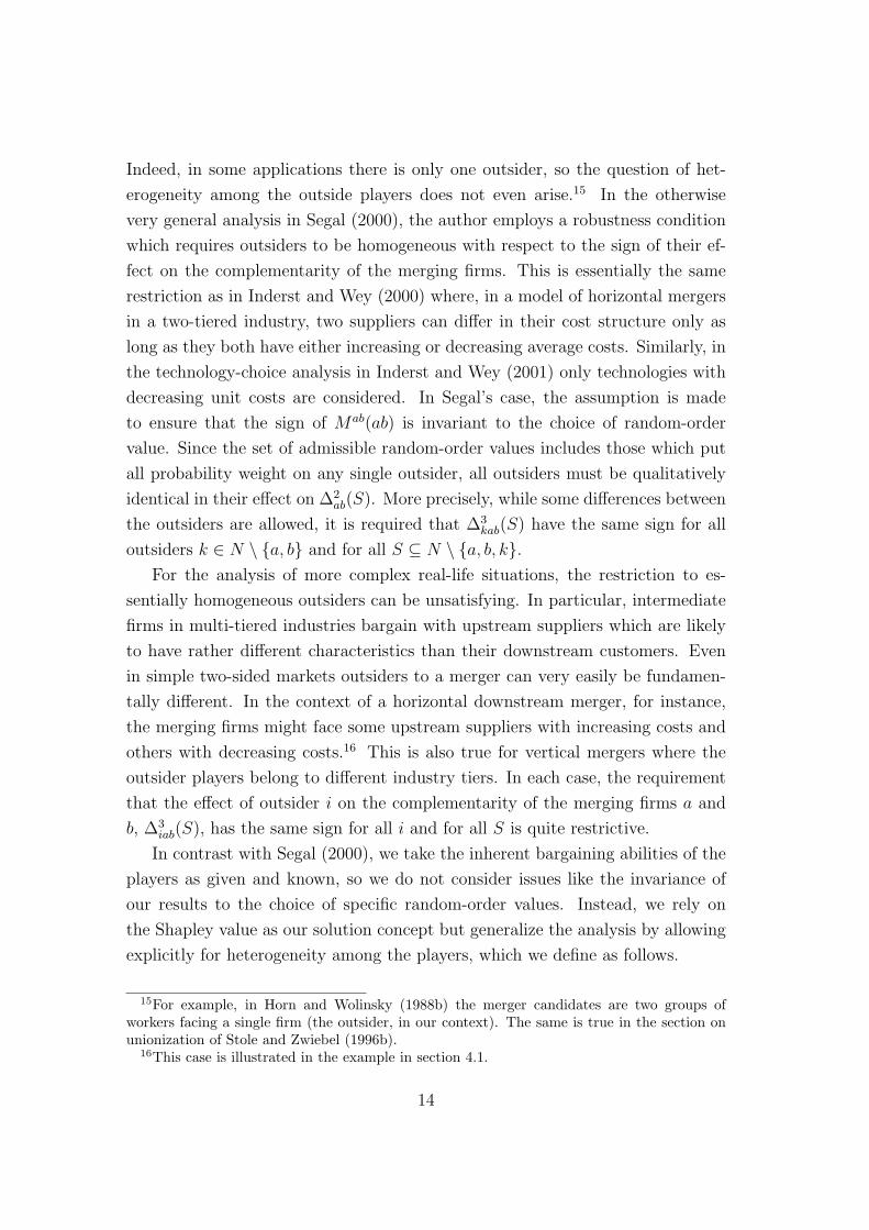
4.1 Example: Horizontal Merger in a Retailing Model

Consider the horizontal-merger decision of two retailers a and b facing two pro-

ducers c and d in a four-firm industry a la Inderst and Wey (2001) illustrated

in Figure 1. Let xac denote the quantity supplied to retailer a by producer c,

and analogously for the other three trading links. The cost function of producer

i = c, d is given by

κi(xai + xbi) + δi(xai + xbi)2, κi ≥ 0.

To introduce the kind of fundamental heterogeneity defined above, we assume

that δc > 0 and δd ∈ (−12, 0), implying increasing unit costs for producer c

20

c d

a b

Figure 1: Two retailers a and b selling the output of both upstream producers cand d in separate local markets.

and decreasing costs for producer d. Each retailer i = a, b operates as a local

monopolist, achieving a gross profit (before payments to the upstream suppliers)

of

α(xic + xid)− (x2ic + x2

id), α > max{κc, κd}

from selling the two goods.20 At least one retailer and one producer must be

present for a coalition of firms to achieve a positive profit; this implies that

∆2ab(∅) is zero. Hence, if a and b merge, then the merger benefits to the outsiders

c and d are21

M c(ab) =1

12

(∆2

ab(c)−∆2ab(d) + ∆2

ab(cd))

(10)

and

Md(ab) =1

12

(∆2

ab(d)−∆2ab(c) + ∆2

ab(cd)), (11)

while the merging firms improve their joint payoff by

Mab(ab) = −1

6∆2

ab(cd).

Maximizing joint profits over the quantities traded among each coalition of

firms gives

∆2ab(c) = v(abc)− v(ac)− v(bc)

= − δc(α− κc)2

2(1 + δc)(1 + 2δc),

(13)

∆2ab(d) = v(abd)− v(ad)− v(bd)

= − δd(α− κd)2

2(1 + δd)(1 + 2δd),

(14)

20The gross-profit function implies that the goods are neither (strict) substitutes nor com-plements, and that the retailers have no operating cost. Neither assumption is critical. Thelocal-monopoly assumption conveniently eliminates coordination problems for a and b vis-a-visfinal consumers (but not against c and d).

21Cf. (6)–(8)

21

and

∆2ab(cd) = v(abcd)− v(acd)− v(bcd)

= − δc(α− κc)2

2(1 + δc)(1 + 2δc)− δd(α− κd)

2

2(1 + δd)(1 + 2δd)

= ∆2ab(c) + ∆2

ab(d).

(15)

(The equality of ∆2ab(cd) = ∆2

ab(c) + ∆2ab(d) stems from the fact that the down-

stream goods are neither complements nor substitutes; this is convenient but not

critical for this example.)

Since δc > 0 and δd < 0 by assumption, we have ∆2ab(c) < 0 and ∆2

ab(d) > 0.

By (10), (11) and (15), the merger benefit is negative for the increasing-cost

outsider c and positive for supplier d: M c(ab) = 2∆2ab(c) < 0 and Md(ab) =

2∆2ab(d) > 0. Thus, the upstream firms are heterogeneous according to Definition

2, and they satisfy condition (9) for all permissible values of α, κc and κd.22 As a

consequence of Corollary 1, when the merger incentive for a and b is close to zero,

one of the outsiders receives most of the redistributed surplus. Indeed, one can

easily find parameter values such that ∆2ab(d) = −∆2

ab(c) > 0, in which case a and

b are indifferent about merging, and the merger effectively redistributes surplus

from the increasing-cost producer c to the supplier d operating a decreasing unit

cost.

Now suppose that initially the merger candidates a and b prefer to stay apart,

i. e. Mab(ab) < 0 because ∆2ab(cd) = ∆2

ab(c) + ∆2ab(d) > 0. Suppose further that

producer d is hit by a negative cost shock increasing κd by λ, which, other things

equal, has a continuous, negative impact on d’s Shapley value Shd. At the same

time, the shock leaves ∆2ab(c) < 0 unchanged but decreases ∆2

ab(d) arbitrarily close

to zero.23 Thus, player d increases the complementarity between a and b by less

than before the shock. This affects the trade-off for the merger candidates a and b

between extracting more rent from c by merging and from d by staying separate,

and if λ is large enough, then a and b reverse their initial decision and merge. As

a function of λ, therefore, player d’s total payoff is non-monotonic. Precisely, it

is decreasing except for an upward jump at the point where ∆2ab(d) = −∆2

ab(c),

at which the merger becomes profitable. If ∆2ab(d) was close to −∆2

ab(c) before

the shock and the shock is not too large, then by the continuity of v, the negative

22∆2ab(d) > ∆2

ab(c) implies ∆3dab(∅) ≡ ∆2

ab(d) − ∆2ab(∅) > ∆3

cab(∅) ≡ ∆2ab(c) − ∆2

ab(∅) for allκc < α and κd < α.

23The derivative of ∆2ab(d) w. r. t. κd is negative for κd ∈ [0, α), and ∆2

ab(d) → 0 as κd → α.

22

effect on Shd is less than the merger benefit Md(ab), and player d benefits overall

from the negative shock, while player c suffers (since M c(ab) < 0). It is worth

noting that the negative effect of a shock to supplier d is borne primarily by the

increasing-cost supplier c which is connected to d only through their common

downstream customers.

Instead of being subject to an exogenous shock, player d might have to make

a binding technology choice before a and b decide about merging. The range

of negative-shock sizes leaving d better off overall then translates into a range

of technology parameters such that d’s final payoff is maximized by choosing

an inferior technology lest ∆2ab(d) be so large as to induce a merger of a and

b. By the same line of reasoning, a positive shock specific to player d can be

compensated by an adverse merger decision by a and b, leaving d worse off than

before the shock. This implies a disincentive to engage in cost-reducing R&D for

a player with a positive merger-benefit term Mk(ab), i. e. for a trading partner

which enhances the complementarity of a and b. For instance, the incentive for

a decreasing-cost supplier to reduce its marginal cost is inefficiently low if one of

its customers responds by de-merging into two independent units.

5 Interaction Between Merger Decisions

So far we have only considered a single merger of two predetermined players. In

this section, we analyze the effect of one merger on the profitability of another,

where both pairs of merger candidates are exogenously fixed. While this is still

much less ambitious than allowing for the endogenous determination of merging

partners, we believe it to be a significant building block for a more complete

theory of bargaining and mergers, and for a better understanding of “merger

waves”.

As a stylized empirical fact, it is often observed that mergers occur in waves.

There are several possible explanations for this, from economy-wide shocks in-

creasing the profitability of mergers (like changes in the tax code or in the anti-

trust regime) to herding effects and management fads. Nilssen and Sørgard (1998)

show how mergers can be strategic complements in a Cournot model a la Salant

et al. (1983). While this suggests that market power considerations might lead

to an interaction of merger incentives for disjoint sets of players, this is not dis-

entangled from the monopolization effect and the cost synergies assumed by the

authors. On the other hand, Inderst and Wey (2001) find that merger incentives

23

are independent in a model based purely on bargaining effects.

The results in this section show that even in a pure bargaining model, the

decisions of two disjoint pairs of merger candidates generally interact. Only in

the special case of n = 4, when there are no “complete” outsiders who participate

in neither merger, are pairwise mergers independent of each other. Intuitively,

the merger of two firms a and b affects the impact ∆3kcd(S) of each “complete”

outsider k ∈ N \ {a, b, c, d} on the complementarity of players c and d and,

therefore, the amount of surplus Mk(cd) received by those outsiders when c and

d merge. This is because some of the preceding coalitions S contain a and b, who

after their merger appear either jointly or not all where before they appeared

separately. As will be shown, this leads to a symmetric interaction between the

merger incentives for a and b on the one hand and c and d on the other. The

interaction can be positive, in which case mergers are strategic complements; if

it is negative, they are strategic substitutes.

Let a and b denote two players pondering a merger, and let c and d denote

a disjoint second pair of potential merger candidates, so that {a, b} ∩ {c, d} = ∅and {a, b} ∪ {c, d} ⊆ N . Only the a–b merger and the c–d merger are allowed; in

particular, the firms cannot form a grand merger containing all four of them. We

first look for the effect of a merger of a and b on the private profitability M cd(cd)

of the c–d merger. This is the same as the negative sum of the effects of the a–b

merger on the merger benefits Mk(cd) received by all outsiders k ∈ N \ {c, d}when c merges with d. Among the outsiders to the second merger are the players

who have formed the first; of these, a is again, and without loss of generality,

treated as the proxy player while b is taken to be a dummy. The a–b pair needs

to be considered separately from those players k /∈ {a, b, c, d} who participate in

neither merger, because after their own merger, a and b contribute a different

set of marginal resources to the same preceding coalitions, while the “complete”

outsiders k ∈ N \ {a, b, c, d} contribute the same resources as before to different

preceding coalitions.

The two types of outsiders are considered in turn before the total effect of the

a–b merger on M cd(cd) is stated in Proposition 3.

5.1 k 6∈ {a, b, c, d}

We begin with the “complete” outsiders, restricting our attention to those or-

derings where c ≺π k ≺π d, i. e. k follows c and precedes d, which are the only

24

relevant ones for

Mk(cd) =1

n!

∑π∈Π

1[c ≺π k ≺π d]∆kcd(B′(k, π)), (16)

where

B′(k, π) ≡ B(k, π) \ {c, d},

like before, stands for the set of outsiders to the c–d merger who precede player

k in ordering π.

If both a and b precede k in ordering π, then the a–b merger has no relevant

effect on the k-preceding coalition B′(k, π).24 The same is true when both a and

b appear after k. This leaves those orderings where k comes between {a, b} and

{c, d}.If {a, c} ≺π k ≺π {b, d}, then after the a–b merger, the relevant preceding

coalition is B′(k, π)∪ b instead of just B′(k, π). Conversely, when {b, c} ≺π k ≺π

{a, d}, the post-merger preceding coalition is B′(k, π) \ b rather than B′(k, π).

These two cases can be pairwise combined and aggregated quite concisely with

the help of some additional notation.

Define the set of preceding players outside of both merger pairs as

B′′(k, π) ≡ {i ∈ N \ {a, b, c, d} : i ≺π k}≡ B′(k, π) \ {a, b}.

(17)

For each ordering π ∈ Π with a ≺π k ≺π b there is exactly one corresponding

ordering π∗ ∈ Π which differs only in the transposition of a and b. In particu-

lar, the set of “complete” outsiders preceding k is the same in both orderings,

B′′(k, π) = B′′(k, π∗). Thus, the effects in the two relevant types of orderings can

written as

1

n!

∑π∈Π

1[{a, c} ≺π k ≺π {b, d}][∆3

kcd(B′′(k, π) ∪ {a, b}) + ∆3

kcd(B′′(k, π))

−∆3kcd(B

′′(k, π) ∪ a)−∆3kcd(B

′′(k, π) ∪ b)].

(18)

This is the average complementarity of a and b as members of the coalition

B′(k, π) preceding k, for ∆3kcd(B

′(k, π)). Intuitively, the complementarity of a

24Recall that only the identity of the players in B′(k, π) matters for ∆3kab(B

′(k, π); theirordering within B′(k, π) is irrelevant. Moreover, adding the dummy player to B′(k, π) has noeffect.

25

and b matters because after their merger, they appear either in combination or

not at all, where before they would contribute their resources separately. This

is emphasized in the following representation of (18) using the second-difference

operator ∆2ab.

Lemma 3 The effect of the a–b merger on the c–d merger benefit for each “com-plete” outsider k ∈ N \ {a, b, c, d} in (18) is equivalent to

1

n!

∑π∈Π

1[{a, c} ≺π k ≺π {b, d}]∆2ab

(∆2

cd [B′′(k, π) ∪ k]−∆2cd [B′′(k, π)]

)(19)

This follows directly from the definition of the difference operators ∆2ab and ∆3

kcd.

The next step is to aggregate the effect in (19) across all “complete” outsiders

k ∈ N \ {a, b, c, d}. To do this, we can exploit the fact that (19), and hence

the sum over all outsiders, consists of terms of the form ∆2ab(∆

2cd(S)), where

S ⊆ N \ {a, b, c, d}. Therefore, the total effect on all complete outsiders can

be computed by adding over all subsets S ⊆ N \ {a, b, c, d}, which leads to a

particularly simple expression.

Lemma 4 Across all “complete” outsiders k ∈ N \ {a, b, c, d}, the effect of thea–b merger on the benefits Mk(cd) received from the c–d merger is

− 2

n!

∑S⊆N\{a,b,c,d}

α|S|∆2ab

[∆2

cd(S)], (20)

where the coefficient

α|S| = (n− 2|S| − 4) (|S|+ 1)! (n− |S| − 3)! (21)

depends only on n and the cardinality of S.

We postpone the discussion of α|S|, which has some interesting characteristics,

and of the nested second differences, until Proposition 3 has been derived.

5.2 k ∈ {a, b}

The merging players a and b need to be considered separately as outsiders to the

merger of c and d because they change their marginal contribution to any given

preceding coalition. Consider first the dummy player b. If a and b stay apart,

then the effect of the c–d merger on the payoff of b is

M b(cd) =1

n!

∑π∈Π

1[c ≺π b ≺π d]∆3bcd(B

′(b, π)). (22)

26

In contrast, when a and b have merged and b has become a dummy player, the

effect of the c–d merger on b is zero by definition. Thus, by participating in

the first merger with a, player b loses ∆3bcd(B

′(b, π)) in each ordering π with

c ≺π b ≺π d. (The loss may well be negative, i. e. a gain.)

The proxy player a, on the other hand, receives a c–d merger benefit (if

positive; damage if negative) of

Ma(cd) =1

n!

∑π∈Π

1[c ≺π a ≺π d]∆3acd(B

′(a, π)) (23)

if a and b are separate players, and

M (ab)(cd) =1

n!

∑π∈Π

1[c ≺π a ≺π d]∆3(ab)cd(B

′(a, π)) (24)

when they are merged, where the (ab) notation indicates that a now controls the

joint resources of a and b.

Our objective for the moment is to determine how the combined c–d merger

benefits for a and b change when a and b merge themselves. Formally, we look

for

M (ab)(cd)−Ma(cd)−M b(cd). (25)

Since M (ab)(cd), Ma(cd), and M b(cd) contain different third-difference terms eval-

uated over various preceding coalitions in different subsets of Π, solving for the

aggregate effect in (25) involves a number of steps. First, the fundamental sym-

metry of the permutations in Π allows us to sum the terms in M b(cd) over the

equivalent orderings with c ≺π a ≺π b obtained by the transposition of a and b

in each ordering π in (22). Second, the third-difference terms ∆3icd(B

′(i, π)) can

be expressed in terms of second differences ∆2cd(·) and sets of complete outsiders

B′′(a, π) preceding a, so that each of the merger benefits in (25) can be written

as a sum of comparable terms. The following lemma describes the result of these

operations. The proof in Appendix B contains the details.

Lemma 5

M (ab)(cd)−Ma(cd)−M b(cd) =

1

n!

∑π∈Π

{1[c ≺π a ≺π {b, d}

]∆2

ab

(∆2

cd[B′′(a, π)]

)− 1

[{b, c} ≺π a ≺π d

]∆2

ab

(∆2

cd[B′′(a, π)]

)}.

(26)

27

As before, this expression can be rewritten as the sum of terms of the form

∆2ab(∆

2cd(S)) over all coalitions S ⊆ N \ {a, b, c, d} of preceding outsiders.

Lemma 6 The effect in (26) of the merger of players a and b on their own benefitderived from a merger of players c and d is equivalent to

1

n!

∑S⊆N\{a,b,c,d}

α|S|∆2ab

[∆2

cd(S)], (27)

with α|S| as defined in (21).

5.3 Total effect of the first merger on the second

The total effect of the merger of a and b on the profitability of the c–d merger is

the negative sum of (20) and (27).

Proposition 3 The effect of the merger of a and b on the profitability M cd(cd)of the c–d merger is given by

1

n!

∑S⊆N\{a,b,c,d}

α|S|∆2ab

[∆2

cd(S)], (28)

with α|S| as defined in (21).

A number of points are worth noting about the coefficients α|S|. First, they

depend only on n and on the size of each coalition S ⊆ N \ {a, b, c, d}. Second,

they are positive for S = ∅, negative for S = N \ {a, b, c, d}, and non-increasing

in |S|. Third, they are symmetric in the sense that

α|S| = −αn−|S|−4,

so that for each S of size |S| there is a corresponding S ′ ⊆ N \ {a, b, c, d} of size

n− |S| − 4 whose coefficient is minus that of S.

For example, for n = 5 and N = {a, b, c, d, e}, (28) becomes

1

120

(2∆2

ab

[∆2

cd(∅)]− 2∆2

ab

[∆2

cd(e)])

=− 2

120∆2

ab

[∆3

ecd(∅)]

=− 2

120∆2

ab

[∆2

cd(∆e(∅))]

(29)

Hence, the a–b merger increases the profitability of the c–d merger if and only

if a and b are non-complementary in their effect on ∆3ecd(∅). Recall that when c

28

and d merge, some of the redistributed surplus goes to e if ∆3ecd(∅) > 0, i. e. if e

enhances the complementarity of c and d. In order to make the c–d merger more

attractive, the merger of a and b—in essence, the decision to act in combination

rather than separately—must reduce this third-difference term, which is just what

(29) implies.25

When n > 5, (28) expands to a sum of terms of the form

−∆2ab

[∆2

cd(S′)−∆2

cd(S)],

where S is a strict subset of S ′. The term in square brackets describes the impact

of the players in S ′ \ S on the complementarity of the merging parties c and d;

this corresponds to the third-difference terms in (16) describing the impact of

a single outsider on the complementarity of the merging firms. Hence, it is a

measure of the amount of surplus redistributed to outsiders when c and d merge.

To increase the profitability of the merger of c and d, the first merger of a and b

must reduce the amount of surplus going to outsiders. It does so if and only if a

and b are non-complementary with respect to the term in square brackets, i. e. if

and only if ∆2ab[ · ] is negative.

Among other things, Proposition 3 implies that there is no effect of the first

merger on the second when there are no other players besides {a, b, c, d}. In

contrast, the two merger decision are generically interdependent when n > 4.

Thus, while four-player models might appear to be a natural starting point for

the analysis of two disjoint mergers, their results do not necessarily generalize to

a setting with n > 4.

Corollary 3 (n = 4) Disjoint pairwise mergers are independent if n = 4. Theyare generically interdependent if n > 4.

Another implication of (28) is the fundamental symmetry of the interaction

between disjoint mergers.

Corollary 4 (Symmetry of merger interaction) The impact of a merger ofa and b on the profitability of a merger between c and d is the same as the effectof the c–d merger on the profitability of the merger of a and b.

This symmetry follows from the fact that ∆2ab(∆

2cd(S)) = ∆2

cd(∆2ab(S)), i. e. that

the order of taking differences over v(S) is irrelevant. Abusing terminology, one

25Cf. the discussion in Section 5.4 of the solid curve in Figure 3

29

can think of ∆2cd(S) as the first derivative of the characteristic function with

respect to the (binary) merger decision of c and d, evaluated at S. By the same

token, ∆2ab(∆

2cd(S)) corresponds to the cross-derivative of v with respect to both

mergers, so that the symmetry of interaction between them is not surprising.

Proposition 4 follows directly.

Proposition 4 Merger decisions are strategic complements if (28) is positive. Asufficient condition is that ∆2

ab(∆2cd(S)) is non-increasing in the cardinality of S

for all S ⊆ N \ {a, b, c, d}.Conversely, mergers are strategic substitutes if (28) is negative, for which it

is sufficient that ∆2ab(∆

2cd(S)) is non-decreasing in the cardinality of S for all

S ⊆ N \ {a, b, c, d}.

The intuition behind the sufficient conditions in Proposition 4 is that, if

∆2ab(∆

2cd(S)) is non-increasing in S, then ∆2

ab(∆3kcd(S)) ≡ ∆2

ab(∆2cd(S∪k)−∆2

cd(S))

is non-positive for all outsiders k ∈ N \ {a, b, c, d}, k /∈ S. Thus, the third-

difference terms which sum to k’s merger benefit Mk(cd) in (16) are weakly re-

duced by the merger of a and b, and hence the share of surplus received by c and

d after their merger increases. Conversely, if ∆2ab(∆

2cd(S)) is non-decreasing in S,

then the a–b merger increases Mk(cd) for all outsiders k, reducing the incentive

for c and d to merge as well.

The fact that merger decisions can be either strategic substitutes or comple-

ments gives rise to a familiar kind of considerations.26 In particular, the inter-

action of merger decisions implies a rationale for merger waves based entirely on

bargaining considerations. When two pairwise mergers are unprofitable in isola-

tion but profitable if undertaken simultaneously, then the removal of an obstacle

blocking only one of them (an easing of sector-specific regulation, say) can trig-

ger a merger of firms which, prima facie, should not have been affected by that

obstacle before.

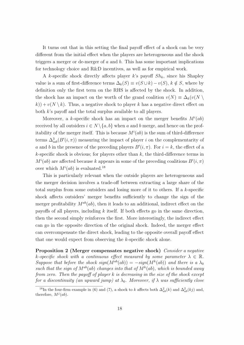
5.4 Example: Vertical mergers in a three-tiered industry

As an example for the interaction between disjoint pairwise mergers, consider the

simple extension of the Inderst–Wey retailing model from section 4.1 illustrated

in Figure 2. As before, there are two local-monopoly retailers selling the goods

produced by two suppliers. For consistency with the notation used in section 5,

26See, e. g., Bulow et al. (1985). Nilssen and Sørgard (1998) apply the “puppy dog/fat cat”framework of Fudenberg and Tirole (1984) to the analysis of sequential mergers in a Cournotoligopoly.

30

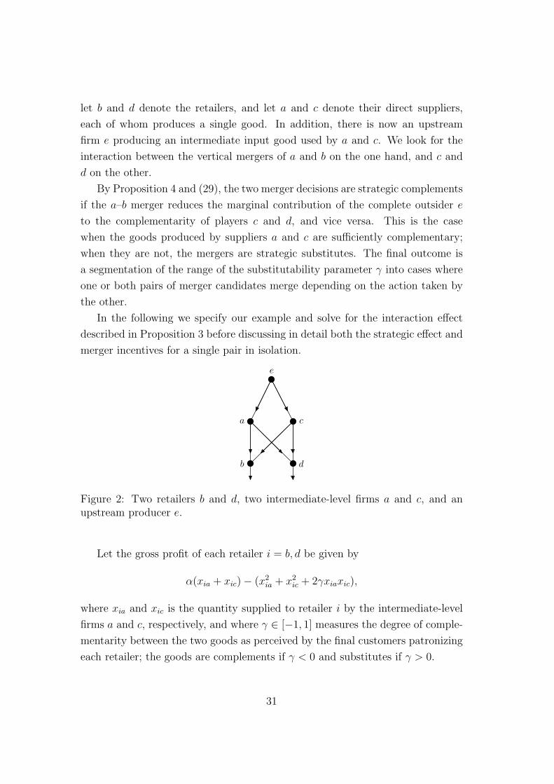
let b and d denote the retailers, and let a and c denote their direct suppliers,

each of whom produces a single good. In addition, there is now an upstream

firm e producing an intermediate input good used by a and c. We look for the

interaction between the vertical mergers of a and b on the one hand, and c and

d on the other.

By Proposition 4 and (29), the two merger decisions are strategic complements

if the a–b merger reduces the marginal contribution of the complete outsider e

to the complementarity of players c and d, and vice versa. This is the case

when the goods produced by suppliers a and c are sufficiently complementary;

when they are not, the mergers are strategic substitutes. The final outcome is

a segmentation of the range of the substitutability parameter γ into cases where

one or both pairs of merger candidates merge depending on the action taken by

the other.

In the following we specify our example and solve for the interaction effect

described in Proposition 3 before discussing in detail both the strategic effect and

merger incentives for a single pair in isolation.

a c

b d

e

Figure 2: Two retailers b and d, two intermediate-level firms a and c, and anupstream producer e.

Let the gross profit of each retailer i = b, d be given by

α(xia + xic)− (x2ia + x2

ic + 2γxiaxic),

where xia and xic is the quantity supplied to retailer i by the intermediate-level

firms a and c, respectively, and where γ ∈ [−1, 1] measures the degree of comple-

mentarity between the two goods as perceived by the final customers patronizing

each retailer; the goods are complements if γ < 0 and substitutes if γ > 0.

31

Let the intermediate-level firms a and c produce each unit of their differ-

entiated goods using as their only input one unit of the homogeneous out-

put of the upstream firm e.27 Firm e, in turn, produces the total quantity

xae + xce ≡ xba + xbc + xda + xdc at increasing, quadratic cost

δ(xae + xce)2 δ > 0.

We assume that each tier of firms is essential, i. e. a coalition of firms can only

produce some final output if it contains player e, plus at least one of a and c,

plus at least one of b and d.28 Standard computations show that the worth of the

grand coalition N = {a, b, c, d, e} is equal to

v(abcde) =α2

1 + 4δ + γ,

which is well-defined for all δ > 0 and γ ≥ −1. Total output is

xba + xbc + xda + xdc =2α

1 + 4δ + γ.

Now consider the strategic effect of a vertical merger of firms a and b on the

profitability of a second merger of c and d. By (29) and the maximization of the

relevant subcoalition payoffs, this is equal to

− 2

120∆2

ab

[∆3

cde(∅)]

=− 2

120α2

(1

1 + δ+

1

1 + 4δ + γ− 1

1 + 2δ− 1

1 + 2δ + γ

). (30)

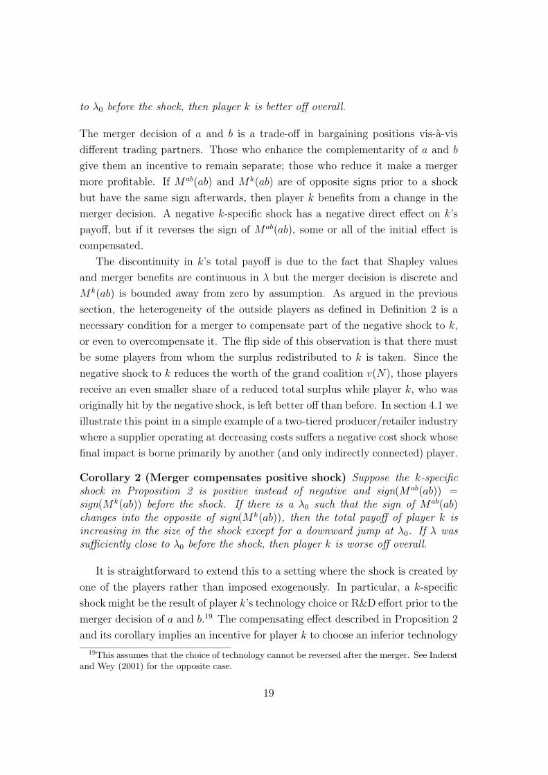
As noted above, this is a mutual effect of each vertical merger on the profitability

of the other. The right-hand side of (30) is the continuous, decreasing function

of the substitutability parameter γ shown as the solid curve in Figure 3. It is

positive when the goods are perfect complements (γ = −1) and negative when

they are perfect substitutes (γ = 1). Thus, the two vertical-merger decisions are

strategic complements if and only if the goods produced by the intermediate firms

are sufficiently complementary (precisely, if γ is lower than the unique value γ0

at which (30) is zero).

27Endowing the intermediate firms with a proper production function has no qualitative effecton our results.

28This assumption simplifies the analysis by reducing the worth of some subsets of N to zero;it is not critical.

32

γ−1 10γ2 γ1

γ0 γ3

Figure 3: Profitability of a vertical merger in isolation (broken line), and mu-tual effect of one merger on the other (solid line). The two goods are perfectcomplements when γ = −1 and perfect substitutes when γ = 1. The vertical axisindicates utils. α = 2 and δ = .3

In the example drawn in Figure 3 with α = 2 and δ = .3, the range of

substitutability parameters γ is segmented into four cases. First, when γ ∈[−1, γ2] (the goods are close complements), then c and d profit from merging

regardless of the decision taken by the other merger candidates (but their total

profit is higher if a and b also merge).

Second, when γ ∈ (γ2, γ1] then the merger of c and d is profitable if and

only if a and b merge as well: The broken curve is negative but the sum of

both curves is positive. By the fundamental symmetry of this simple model,

the incentives for a and b are exactly the same, and it is precisely the strategic

complementarity of the two mergers which makes each of them profitable if both

occur. Essentially, this leads to a simple (2 × 2) normal-form game with two

symmetric, Pareto-ranked equilibria in which both pairs of players take the same

action. It is straightforward to think of real-life situations where one of the two

pairs is prevented by some exogenous force from taking the prefered merger (or de-

merger) decision; when this obstacle is removed, both pairs or merger candidates

act in unison even though only one of them is directly affected by it. Hence, even

in this simple illustration can one find a purely bargaining-based rationale for a

merger/de-merger “wave”.

Third, when γ ∈ (γ1, γ3], neither pair of candidates wants to merge no matter

what action is taken by the other. Finally, when the goods are very close sub-

33

stitutes and γ ∈ (γ3, 1], the c–d merger (and, by symmetry, the a–b merger as

well) is profitable if and only if the other merger does not take place. While this

implies the usual kinds of coordination problems, it is another instance where the

reversal of either merger decision leads to a change of the other.

In the remainder of this section, we describe the forces behind these effects in

more detail. To develop an intuition for the mutual effect in (30), it is useful first

to consider the broken curve in Figure 3 representing the merger profitability for

c and d, M cd(cd), when players a and b remain separate. This is the negative sum

of the effects of the c–d merger on each of the remaining three players. Formally,

M cd(cd) = −[Ma(cd) + M b(cd) + M e(cd)

]. (31)

Consider the three terms on the RHS in turn. The effect Ma(cd) on player

a is a decreasing function of the substitutability parameter γ. Intuitively, the

merger of c and d results in a shift towards the margin of the negotiation over

the joint rent with player a as a supplier to retailer d. The more substitutable

the goods produced by a and c, the lower is the marginal rent relative to the

inframarginal one which c and d “lock in” by merging.29 In contrast, the merger

benefit M b(cd) for retailer b is a negative, concave and increasing function of γ.

The c–d merger shifts the negotiation between retailer b and supplier c to the

margin where rents are lower due to the convexity of the upstream firm’s costs.30

This effect is more pronounced when output (and hence, marginal cost) is high,

which is the case when γ is low and the goods are complements. Conversely,

total output falls in γ, so when the goods are more substitutable, marginal costs

are relatively lower and the c–d merger is less detrimental to retailer b. Finally,

the merger benefit M e(cd) of the upstream firm e is a positive function which

monotonically decreases in γ. Being an essential player, e always increases the

complementarity of c and d. The more complementary the goods produced by

the intermediate firms a and c, the higher is the worth of the grand coalition

v(N) and the larger is the average contribution of the upstream firm e to the

complementarity of the players c and d, and hence, M e(cd).

Overall, (31) is a quasiconvex function of γ on [−1, 1] which is decreasing

at γ = −1. If δ < 1/2, then there is an interval [γ, γ], −1 ≤ γ < γ ≤ 1, on

which (31) is negative.31 Otherwise, it is positive throughout. Intuitively, when

29This is closely related to the “scarce needs” variant of the vertical-foreclosure model ofHart and Tirole (1990).

30Cf. the “scarce supplies” variant in Hart and Tirole (1990).31In Figure 3, this interval is given by [γ2, γ3].

34

the goods are close complements, then the negative effect of the c–d merger on

retailer b dominates the effects on the other two outsiders, so that c and d profit

from merging. Moreover, when the cost parameter δ is large (> 1/2), the effect on

b dominates regardless of the substitutability between the goods, and the merger

of c and d is profitable in isolation for all values of γ.

Now consider the solid curve in Figure 3 depicting the strategic effect of a

merger of players a and b on the profitability of the c–d merger. After a and b

have merged, they employ or withdraw their joint resources together rather than

separately. Thus, the merger of a and b eliminates those bargaining situations

where the upstream firm e makes its marginal contribution to a set of players

containing only a or b but not the other. As it turns out, this implies that the

merger benefit from the c–d merger for the upstream firm, M e(cd), is reduced

when the goods are complements and increased when they are substitutes.

To see this, consider the terms which make up M e(cd) when a and b are

separate players. Recall that

M e(cd) =1

n!

∑π∈Π

1[c ≺π e ≺π d]∆e

[∆2

cd(B′(e, π))

].

The preceding coalitions B′(e, π) are {∅}, {a, b}, {a}, and {b} (with different but

positive weights). In the absence of the intermediate firm a, there is no second

good, and both ∆e(∆2cd(∅)) and ∆e(∆

2cd(b)) are positive but independent of the

substitution parameter γ. In contrast, γ has an important effect for ∆e(∆2cd(a))

and ∆e(∆2cd(ab)).

∆e(∆2cd(a)) represents a bargaining situation where retailer b is not active; the

term is positive and monotonically decreasing in γ ∈ [−1, 1) and zero for γ = 1.

With complementary goods, the essential player e enables c and d to generate

together, but not separately, a positive profit which increases as the total value

of the final output increases (i. e. as γ decreases and the goods become more

complementary). In contrast, as γ goes to unity and the goods become perfect

substitutes, player c no longer provides any additional value when its competitor

a is present, so that c and d are no longer complementary players.

On the other hand, ∆e(∆2cd(ab)) determines the bargaining share of the up-

stream firm e when all other players are active as well; it is negative when the

goods are close complements, i. e. the joint contribution of supplier c and retailer

d to the remaining three players is less than the sum of their individual contribu-

tions. This is because a second retailer adds no value when the two intermediate

35

firms a and c supply perfect complements produced (or procured) at increasing

cost. The marginal value of an additional unit is then equal to α at either re-

tailer independent of absolute quantities, so adding d as a second retailer does

not increase the worth of coalition {a, b, c, e}. In contrast, retailer d does make a

positive contribution when supplier c is absent, since without the complementary

good produced by c, the marginal value α − 2xia of supplier a’s output xia is

strictly decreasing in each local retailing market. Hence, supplier c reduces the

marginal contribution of retailer d when the goods are close complements, result-

ing in a weak bargaining position for the essential upstream firm e. When the

goods are perfect substitutes, in contrast, the marginal contribution of supplier

c is zero whenever its competitor a is already present, so that ∆e(∆2cd(ab)) = 0

for γ = 1.

When a and b merge, the upstream firm e bargains either in the presence of the

merged entity or in the absence of both a and b. Technically, the third-difference

terms ∆e(∆2cd(a)) and ∆e(∆

2cd(b)) are replaced by ∆e(∆

2cd(∅)) and ∆e(∆

2cd(ab)).

Since ∆e(∆2cd(b)) and ∆e(∆

2cd(∅)) are constant in γ, and since

∆e(∆2cd(a))−∆e(∆

2cd(ab))

is positive and monotonically decreasing in γ, the merger of a and b reduces the

bargaining power of the upstream firm e if the goods are complementary (i. e. if

γ is low). The upshot is that the mutual effect of the two disjoint mergers on

each other represented by the solid curve in Figure 3 is a decreasing and convex

function of γ which, for δ > 0, is positive at γ = −1 and negative at γ = 1.

Hence, there is a unique value γ0 ∈ (−1, 1) such that the merger decisions of

the two pairs of candidates are strategic complements if γ < γ0 and strategic

substitutes otherwise.

When each pair of merger candidates takes into account the strategic effect

in (30) in addition to the direct effect of their decision in (31), then the range

of values of the substitutability parameter γ ∈ [−1, 1] is segmented into different

cases as a function of the sum of both effects as described above. Depending

on parameter values, however, some of the cases described above may not exist.

For instance, when the cost parameter δ is larger than 1/2, then M cd(cd) (the

broken curve in the graph) is positive for all admissible values of γ, eliminating

the interesting case where each merger takes place if and only if the other does

as well.

36

6 Conclusion

By explicitly allowing for the heterogeneity of outside players, we extend the

cooperative approach of Segal (2000) in an aspect which seems to be particu-

larly relevant for the study of merger decisions. Real-life industries with bilateral

bargaining are usually more complex than the two-tier models analyzed in most

of the literature. In particular, intermediate-level firms face both upstream and

downstream trading partners, making the assumption of essentially homogeneous

outsiders rather questionable. Even in simple two-sided industries, outsider het-

erogeneity can arise quite naturally, as our four-firm retailing example demon-

strates. Indeed, from a bargaining perspective the salient feature of a multi-tiered

industry is not the number of tiers or the direction of supply flows but the funda-

mental heterogeneity of the players with respect to their marginal contribution

to any given coalition.

When outsiders are heterogeneous, a profitable merger can benefit some of

them even in a pure bargaining model without the monopolization effects typical

for Cournot-market mergers a la Salant et al. (1983). In those models, the merging

firms actually lose market power relative to the outsiders, but the merger reduces

the coordination problem among the Cournot competitors and moves the industry

closer to the cartel outcome; hence, the merging firms receive a smaller share of

a larger pie, and the net effect can go in either direction. In contrast, in our

purely bargaining-based model (like in Segal (2000) and Inderst and Wey (2001)),

the players can coordinate on maximizing total profit regardless of the market

structure, and mergers are all about bargaining power and the distribution of

the fixed surplus. The novel feature in this paper is that mergers lead to a

redistribution among the outsiders as well as from all outsiders to the merging

firms. In particular, the main share of the redistributed surplus can be received

by (some) outsiders.

The fact that outsiders can benefit from a profitable merger is of particular

interest when, prior to the merger decision, an outsider k receives an exogenous

shock to his profitability. Besides the obvious direct payoff effect, such a shock has

an impact on the merger incentives of firms other than k. In particular, the shock

can trigger a merger which overcompensates the direct payoff effect, in which case

the incidence of the shock to one player falls entirely on others who may not even

be directly linked to him. Among other things, this implies inefficient incentives

for (binding) technology choice and R&D effort when a firm’s trading partners

37

subsequently take a merger or de-merger decision.

Finally, we show that the existence of different kinds of outsiders is a neces-

sary and (generically) sufficient condition for the interaction of merger decisions.

If the only outsiders to a merger of two players a and b are the potential par-

ticipants in another, disjoint, merger, then there is no effect of the first merger

on the profitability of the second, and hence no interaction between merger de-

cisions. In contrast, when there are additional outsiders who do not take part

in either merger, then the two pairs of merger candidates interact symmetrically,

turning merger decisions into strategic substitutes or complements. This suggests

a perspective on merger waves which is derived entirely from bargaining consid-

erations: When mergers interact, then an exogenous effect leading to a revision

of one merger decision can affect another, seemingly unrelated one by two other

players in the same industry.

Appendix

A Bargaining and the Shapley value

To motivate our use of the Shapley value, we generalize the stability condition

for multiple bilateral negotiations introduced by Stole and Zwiebel (1996a). Un-

der some additional assumptions, Stole–Zwiebel stability implies that individual

payoffs follow the “fair allocation” rule of Myerson (1980), so by his central result

they are equal to the players’ Shapley values. The additional assumptions (which

are sufficient but not necessary) are (i) “efficient” bargaining sets; (ii) absence

of externalities; and (iii) a mild form of quasi-concavity of the aggregate profit

function.

Myerson shows that individual payoffs in a cooperative game are equal to

Shapley values if (i) the players are connected by chains of “coordination confer-

ences” (trading links, in our terminology), and (ii) the payoff allocation rule is

efficient and fair; it is efficient if individual payoffs sum to the worth of the grand

coalition, and it is fair if eliminating a trading link ij has the same effect on the

payoffs of both players i and j,

Xi(L)−Xi(L \ ij) = Xj(L)−Xj(L \ ij),

for all trading links ij, where Xi and Xj are payoffs and L is the set of all trading

38

links.32

Stole and Zwiebel’s stability condition applies to a setting where three or more

players bargain in bilateral negotiations. Its key feature is the assumption that

contracts are non-binding, so that after the breakdown of any single negotiation

all remaining contracts can be renegotiated. Thus, disagreement payoffs are

given by what the players can achieve by subsequent renegotiations rather than

by what is specified in their expected equilibrium contracts. More precisely, we

define stability as follows.

Definition 4 (Stole–Zwiebel stability) The outcome of a set of simultaneousbilateral negotiations is Stole–Zwiebel (SZ) stable if no player has an incentive tore-open any of his bilateral bargaining sessions, given the contracts specified inall other negotiations, and given that all remaining contracts can be renegotiatedshould the re-opened bargaining session break down in disagreement.

Let n firms N = {1, . . . , n} bargain simultaneously and on a bilateral basis.

Any two firms i and j in N can bargain over a pair of quantities qij ∈ R2+ which

they supply to each other, as well as a net lump-sum payment pij. Thus, allo-

cation and bilateral rent-sharing can be determined separately, so that the issue

of double marginalization does not arise. However, the firms cannot negotiate

anything other than qij and pij. In particular, their behaviour in the remaining

negotiations is not contractible. We follow the literature in assuming that if a

firm is involved in several negotiations, it sends a different agent to each of them.

An agent acts faithfully to maximize the profit of his firm in his bilateral negoti-

ation, but he cannot coordinate his actions with other agents of the same firm.33

Let

Q ≡ {qij}i6=j∈N

denote the set of all bilateral-quantity vectors. Let P denote the corresponding

set of bilateral net payments. Two firms i and j are linked in Q if and only if at

32There are three related types of efficiency in this context. “Efficient bargaining” refersto the fact that when the bargaining set contains both quantities and payments as separateitems, then the bilateral surplus can be shared freely without compromising allocative efficiency.Myerson’s efficiency of the payoff rule means that no surplus is wasted when individual payoffsare determined. Finally, the overall allocation is efficient if it maximizes total surplus acrossall firms.

33The assumption that agents of the same firm cannot communicate is made, for example,by Bjornerstedt and Stennek (2000). A similar notion is implied by the contingent-contractsapproach in Inderst and Wey (2001).

39

least one of the quantities in qij is positive.34 For further reference, let Z ⊆ Q

denote a set of bilateral quantities exogenously set to zero, qij ≡ 0 ⇔ qij ∈ Z.

By abuse of notation, we will also refer to Z as a set of eliminated links ij

corresponding to each qij ∈ Z.

Each firm i ∈ N has a gross profit function fi(Q), defined as its revenue from

sales to customers outside of N minus its own cost of production conditional on

Q, but ignoring payments to and from its trading partners in N . The net profit

gi(Q, P ) of each firm is the sum of fi(Q) and the net payments received from its

trading partners.

In each bilateral negotiation, the two firms i and j choose bilaterally-optimal

quantities qBij to maximize their joint profits, taking the outcomes of all other

bargaining encounters as given,

qBij = arg max

qij

gi(qij, Q−ij, P ) + gj(qij, Q−ij, P ),

where Q−ij is the set of quantities in all other bilateral trades (including those of

i and j with any third party k /∈ {i, j}). In contrast, the bilateral net payment

pij is used to share the incremental joint surplus equally. Under Stole–Zwiebel

bargaining, this is the difference between the joint profit gi(Q, P )+gj(Q,P ) after

an agreement, and the sum of payoffs after a breakdown and the subsequent

renegotiation of all remaining contracts.

Assumption 2 (No externalities) Holding all other elements of Q constant,a change in the bilateral quantity qij only affects the gross profit fk(Q) of firm kif k ∈ {i, j}.

In particular, this assumption rules out production externalities among suppliers,

and it implies that firms do not compete with each other on any market outside

of N .

Lemma 7 Conditional on any set of eliminated links Z ⊆ Q, the allocationmaximizing total surplus across all firms is SZ-stable.

Proof. From a planner’s point of view, a necessary condition for the optimality

of an allocation Q∗ is that for all active links ij /∈ Z,

q∗ij = arg maxqij

∑k∈N

fk(qij, Q∗−ij),

34In the models of buyer-supplier bargaining of which we are a aware, bilateral trade takesplace in only one direction. We allow for two-way trade to emphasize that the equivalence ofShapley values and payoffs under Stole–Zwiebel bargaining generalizes to this case.

40

i. e. each bilateral quantity must maximize industry profits conditional on all

other trades following Q∗. Absent externalities, this is equivalent to

q∗ij = arg maxqij

fi(qij, Q∗−ij) + fj(qij, Q

∗−ij) (32)

for all links ij.

In contrast, players i and j maximize their joint surplus by choosing a bilateral

quantity qij, taking the choices for all other links as given. The bilateral joint

surplus of i and j is maximized by

qBij = arg max

qij

gi(qij, Q−ij, P ) + gj(qij, Q−ij, P ) (33)

for all trading links ij. That is, each bilateral quantity must maximize the sum

of the two parties’ net profits given all other quantities and payments. But

conditional on Q−ij and P−ij, qij affects only gross profits fi(·) and fj(·). (The

bilateral payment pij ∈ P cancels out.) Thus, (33) is equivalent to

qBij = arg max

qij

fi(qij, Q−ij) + fj(qij, Q−ij).

Clearly, this is satisfied by the necessary condition (32) for the planner’s optimal

set of quantities Q∗.

This establishes the SZ stability of the (constrained) efficient outcome after

the breakdown of any number of trading links in the industry. However, bilateral

quantity setting can also lead to SZ stable but inefficient outcomes. An obvi-

ous reason is coordination failure in the presence of complementarities (or scale

economies); another is capacity constraints.35

The following assumptions rule out inefficient equilibria of the bilateral quan-

tity game. The first says that the planner’s optimal set of bilateral quantities is

unique for any given set of links which have been eliminated. In particular, this

rules out perfect substitutes. The second assumption requires that when the set

of quantities is inefficient, at least one pair of firms has an incentive to move its

quantity closer to the efficient quantity q∗ij.

35Suppose there are two buyers and a seller whose marginal cost is zero up to its capacity andinfinite thereafter, let the buyers’ profits be increasing in the amount of the good they receive,and suppose that it is globally efficient for each buyer to receive half the seller’s capacity. In thissituation, any allocation that gives a share of x of the seller’s capacity to one buyer and 1− xto the other is an equilibrium in the game where bilateral quantities are chosen independently.

41

Assumption 3 (Unique efficient quantities) After any set Z ⊆ Q of linkshas been eliminated, total surplus

∑i∈N fi(Q) is uniquely maximized by Q∗

Z.

Assumption 4 A inefficient set of bilateral quantities Q 6= Q∗Z contains at least

one link qij for which∣∣qB

ij − q∗Z,ij

∣∣ <∣∣qij − q∗Z,ij

∣∣, where

qBij = arg max

qij

fi(qij, Q−ij) + fj(qij, Q−ij)

is the bilaterally efficient quantity for firm i and j given Q−ij.

A straightforward way to satisfy the last assumption is to define∑i∈N gi(Q, P )—and thus, by Assumption 2, bilateral joint profits—as continu-

ous and strictly quasi-concave in bilateral quantities, with a maximum in qij > 0

conditional on any Q−ij.36 However, Assumption 4 is less restrictive than that,

allowing for discrete quantities and for some constrained-efficient quantities qBZ,ij

of zero.

So far we have established sufficient conditions for a unique and overall effi-

cient SZ-stable outcome. In each bargaining session, the disagreement points are

given by breakdown payoffs which in turn depend on the payoffs reached after

another link has broken down, and so on until only one active link is left. In other

words, payoffs are determined recursively. Myerson’s result provides a convenient

shortcut which leads directly to the Shapley value.

By assumption, bilateral payments pij are used to share the incremental joint

surplus equally. Thus, if the outcome is SZ-stable, the set of payments P ∗ must

be such that

gi(Q∗, P ∗)− gi(Q

∗Z , P ∗

Z) = gj(Q∗, P ∗)− gj(Q

∗Z , P ∗

Z), (34)

where Q∗Z and P ∗

Z are quantities and payments after a breakdown of the link be-

tween i and j (i. e. Z = {qij}. In words, the payment p∗ij ∈ P ∗ between any trading

partners i and j results in an equal split of their joint profit under the unique

efficient allocation Q∗, minus their payoffs under the unique constrained-efficient,

renegotiated allocation Q∗Z in the event of a breakdown of their bargaining ses-

sion. Condition (34) is nothing other than the “fair allocation” rule of Myerson

(1980) for an arbitrary set of players which are connected through a series of

“conferences” (bilateral bargaining sessions, in our context). As Myerson shows,

the fair-allocation rule plus the fact that payoffs sum to G(Q∗) implies that the

payoff for each player is indeed given by his Shapley (1953) value.

36See, for example, Bjornerstedt and Stennek (2000) or Inderst and Wey (2001).

42

We would like to emphasize, however, that Assumptions 2–4 are sufficient

but not necessary to ensure that SZ-stable payoffs are equal to Shapley values.

Broadly speaking, they ensure that the players can coordinate on the allocation

maximizing their joint surplus even if they only bargain over prices and quantities.

Moreover, they are by no means necessary for our results based on Shapley values

in the main text.

B Proofs

Proof of Lemma 1

M i(ab) and M j(ab) are symmetric sums of third-difference terms ∆3iab(S)

and ∆3jab(S

′), respectively, where S and S ′ are the preceding coalitions

in the relevant orderings where each player follows a but precedes b.

When (9) holds, then the third-difference terms of i exceed those of j

for all preceding coalitions S ⊆ S ≡ N \ {a, b, i, j} containing neither i

nor j. The remaining preceding coalitions are obtained by the union of

each S ⊆ S and {j} for player i and by S ∪ i for player j. Fix some

S∗ ⊆ S. By definition, ∆3iab(S

∗ ∪ j) ≡ ∆2ab(S

∗ ∪ {i, j}) − ∆2ab(S

∗ ∪ j) and

∆3jab ≡ ∆2

ab(S∗ ∪ {i, j}) −∆2

ab(S∗ ∪ i). But ∆2

ab(S∗ ∪ i) ≡ ∆2

ab(S∗) + ∆3

iab(S∗) is

larger than ∆2ab(S

∗ ∪ j) ≡ ∆2ab(S

∗) + ∆3jab(S

∗) by (9). By the symmetry of both

the preceding coalitions and the probability weights of the Shapley value, for

each of the terms over which M j(ab) is summed there is a corresponding and

(weakly) larger term in the sum of M i(ab).

Proof of Lemma 4

Fix a subset S ⊆ N\{a, b, c, d} with cardinality |S|. For each “complete” outsider,

S can appear as an argument in (19) with a positive or negative sign (depending

on whether k ∈ S), corresponding to the preceding coalitions (B′′(k, π) ∪ k) and

(B′′(k, π)) respectively. The coefficient for S in (20) is the net number, across all

outsiders, of preceding coalitions equal to S.

Fix any k ∈ N \ {a, b, c, d}. If k /∈ S, then S corresponds to B′′(k, π) in (19).

Thus, a, c and all the members of S must precede the outsider k in an ordering

π (and all other players must follow k) in order for S to appear, with a negative

sign, in (19). There are (|S|+2)!(n−|S|−3)! such orderings for k, and there are

n− |S| − 4 outsiders k /∈ S. Thus, in the aggregate across all complete outsiders,

43

subset S appears with a negative sign

(n− |S| − 4)(|S|+ 2)!(n− |S| − 3)! (35)

times. Conversely, for each k ∈ S, S corresponds to B′′(k, π) ∪ k in (19), i. e. a,

c and S \ k must precede k in an ordering π so that S appears in (19) with a

positive sign. There are (|S|+ 1)!(n− |S| − 2)! such orderings, and |S| outsiders

in S, giving a total of

|S|(|S|+ 1)!(n− |S| − 2)! (36)

instances where S appears in (19) with a positive sign. The Lemma follows from

netting (35) and (36).

Proof of Lemma 5

M b(cd) can be evaluated over all orderings π ∈ Π with c ≺π a ≺π d, where each π

is obtained from each π with c ≺π b ≺π d in (22) by the transposition of players a

and b. As before, let B′′(b, π) ≡ B′(b, π) \ {a, b} denote the “complete” outsiders

preceding b in ordering π. Consequently, B′′(a, π) = B′′(b, π). If b ≺π a, then

B′(b, π) = B′′(a, π); if a ≺π b, then B′(b, π) = B′′(a, π) ∪ a. Hence,

M b(cd) =1

n!

∑π∈Π

{1[c ≺π a ≺π {b, d}

] (∆2

cd[B′′(a, π) ∪ b]−∆2

cd[B′′(a, π)]

)− 1

[{b, c} ≺π a ≺π d

] (∆2

cd[B′′(a, π) ∪ a]−∆2

cd[B′′(a, π) ∪ {a, b}]

)}.

(37)

Moreover, by the definition of B′′(a, π) ≡ B′(a, π) \ {a, b},

Ma(cd) =1

n!

∑π∈Π

{1[c ≺π a ≺π {b, d}

] (∆2

cd[B′′(a, π) ∪ a]−∆2

cd[B′′(a, π)]

)− 1

[{b, c} ≺π a ≺π d

] (∆2

cd[B′′(a, π) ∪ b]−∆2

cd[B′′(a, π) ∪ {a, b}]

)}(38)

and

Mab(cd) =1

n!

∑π∈Π

{1[c ≺π a ≺π {b, d}

] (∆2

cd[B′′(a, π) ∪ {a, b}]−∆2

cd[B′′(a, π)]

)− 1

[{b, c} ≺π a ≺π d

] (∆2

cd[B′′(a, π)]−∆2

cd[B′′(a, π) ∪ {a, b}]

)}.

(39)

44

Finally,

∆2ab(∆

2cd(S)) ≡ ∆2

cd(S ∪ {a, b}) + ∆2cd(S)−∆2

cd(S ∪ a)−∆2cd(S ∪ b).

The Lemma follows directly.

Proof of Lemma 6

This is analogous to the proof of Lemma 4. The expression in (26) is the sum

of terms of the form ∆2ab∆

2cd(S), where S ⊆ N \ {a, b, c, d} corresponds to the

set of complete outsiders B′′(a, π) preceding player a in ordering π. Fix a subset

S with cardinality |S|. The corresponding term ∆2ab(∆

2cd(S)) has a positive sign

in each ordering where player c and the members of S precede player a (and all

others follow), which is the case in

(|S|+ 1)!(n− |S| − 2)!

orderings. The sign of ∆2ab(∆

2cd(S)) is negative if the coalition preceding a consists

of c, b and S (and no other players); there are

(|S|+ 2)!(n− |S| − 3)!

orderings of this type. Thus, the (net) coefficient corresponding to subset S in

(26) is

α|S| ≡ (n− 2|S| − 4)(|S|+ 1)!(n− |S| − 3)!

References

Bjornerstedt, Jonas, and Johan Stennek (2000). Bilateral oligopoly. Unpublished

manuscript, Research Institute of Industrial Economics (IUI), Stockholm.

Bulow, Jeremy I., John D. Geanakoplos, and Paul D. Klemperer (1985). Mul-

timarket oligopoly: Strategic substitutes and complements. Journal of

Political Economy, 93, 488–511.

Fudenberg, Drew, and Jean Tirole (1984). The fat-cat effect, the puppy-dog ploy,

and the lean and hungry look. American Economic Review, 74, 361–366.

45

Gugler, K., D. Mueller, B. Yurtoglu, and D. Zulehner (2001). The character-

istics and effects of mergers: An international comparison. Unpublished

manuscript, University of Vienna.

Gul, Faruk (1989). Bargaining foundations of Shapley value. Econometrica, 57,

85–95.

Hart, Oliver, and Jean Tirole (1990). Vertical integration and market foreclosure.

Brookings Papers on Economic Activity: Microeconomics, 205–286.

Hart, Sergiu, and Andreu Mas-Colell (1996). Bargaining and value. Economet-

rica, 64, 357–380.

Horn, Henrick, and Asher Wolinsky (1988a). Bilateral monopolies and incentives

for merger. RAND Journal of Economics, 19, 408–419.

Horn, Henrik, and Asher Wolinsky (1988b). Worker substitutability and patterns

of unionisation. Economic Journal, 98, 484–497.

Ichiishi, Tatsuro (1993). The Cooperative Nature of the Firm. Cambridge, UK:

Cambridge University Press.

Inderst, Roman, and Christian Wey (2000). Market structure, bargaining, and

technology choice. Discussion Paper FS IV 00-12, Wissenschaftszentrum

Berlin.

Inderst, Roman, and Christian Wey (2001). Negotiated contracts in bilaterally

oligopolistic industries. Unpublished manuscript, University College Lon-

don and Wissenschaftszentrum Berlin.

Kamien, Morton I., and Israel Zang (1990). The limits of monopolization through

acquisition. Quarterly Journal of Economics, 105, 465–499.

Myerson, Roger B. (1980). Conference structures and fair allocation rules. Inter-

national Journal of Game Theory, 9, 169–182.

Nilssen, Tore, and Lars Sørgard (1998). Sequential horizontal mergers. European

Economic Review, 42, 1683–1702.

Salant, Stephen W., Sheldon Switzer, and Robert J. Reynolds (1983). Losses

from horizontal merger: The effects of an exogenous change in industry

46

structure on Cournot-Nash equilibrium. Quarterly Journal of Economics,

98, 185–99.

Segal, Ilya (2000). Collusion, exclusion, and inclusion in random-order bargain-

ing. Unpublished manuscript.

Shapley, Lloyd S. (1953). A value for n-person games. In Harold W. Kuhn, and

Albert W. Tucker (eds.), Contributions to the Theory of Games, Volume 2,

307–317. Princeton, NJ: Princeton University Press.

Stigler, George J. (1950). Monopoly and oligopoly by merger. American Eco-

nomic Review, 40, 23–34.

Stole, Lars, and Jeffrey Zwiebel (1998). Mergers, employee hold-up and the scope

of the firm: An intrafirm bargaining approach to mergers. Unpublished

manuscript, University of Chicago, GSB, and Stanford University, GSB.

Stole, Lars A., and Jeffrey Zwiebel (1996a). Intra-firm bargaining under non-

binding contracts. Review of Economic Studies, 63, 375–410.

Stole, Lars A., and Jeffrey Zwiebel (1996b). Organizational design and technology

choice under intrafirm bargaining. American Economic Review, 86, 195–

222.

47