basel committee on banking supervision · 5.6 share of the three risk measures ... the basel...
TRANSCRIPT

Basel Committee on Banking Supervision
Analysis of the trading book hypothetical portfolio exercise
September 2014

This publication is available on the BIS website (www.bis.org).
Grey underlined text in this publication shows where hyperlinks are available in the electronic version.
© Bank for International Settlements 2014. All rights reserved. Brief excerpts may be reproduced or translated provided the source is stated.
ISBN 978-92-9131-662-5 (print) ISBN 978-92-9131-668-7 (online)

Contents
Executive summary ........................................................................................................................................................................... 1
1. Hypothetical portfolio exercise description ......................................................................................................... 4
2. Coverage statistics .......................................................................................................................................................... 5
3. Key findings ....................................................................................................................................................................... 5
4. Technical background ................................................................................................................................................... 6
4.1 Data quality .............................................................................................................................................................. 7
4.2 Data processing ...................................................................................................................................................... 7
5. Detailed analysis .............................................................................................................................................................. 8
5.1 Computational assumptions ............................................................................................................................. 8
5.2 Impact of constraining diversification and hedging .............................................................................. 11
5.3 Analysis by asset class ........................................................................................................................................ 12
5.4 The various risk measures ................................................................................................................................ 13
5.5 Implementation of liquidity horizons .......................................................................................................... 15
5.6 Share of the three risk measures (ES, NMRF and IDR) in the total .................................................. 17
5.7 New risk measure compared with the current one ................................................................................ 18
5.8 Variance of each variable through time ..................................................................................................... 19
5.9 Closed form questions ....................................................................................................................................... 19
5.10 Approval status ..................................................................................................................................................... 23
5.11 Stressed period ..................................................................................................................................................... 25
6. Conclusions ..................................................................................................................................................................... 25
Appendix 1: Impact of constraining diversification and hedging ................................................................................ 26
Appendix 2: Analysis by asset class. ......................................................................................................................................... 28
Appendix 3: Analysis of the various risk measures ............................................................................................................ 29
Appendix 4: Implementation of liquidity horizons ............................................................................................................ 39
Appendix 5: Share of the three risk measures ..................................................................................................................... 42
Appendix 6: Portfolio specification for the Hypothetical Portfolio Exercise ............................................................ 43
Analysis of the trading book hypothetical portfolio exercise

Notations used in this report
billion thousand million
The term “country” as used in this publication also covers territorial entities that are not states as understood by international law and practice but for which data are separately and independently available.
iv Analysis of the trading book hypothetical portfolio exercise

Analysis of the trading book hypothetical portfolios exercise
Executive summary
The financial crisis exposed material weaknesses in the capital framework for trading activities. Banks entered the crisis period with insufficient capital to absorb losses. As a rapid response to the undercapitalisation of market risk, the Basel Committee on Banking Supervision introduced a range of revisions to the market risk framework in July 2009 which focused capital requirements on stressed calibrations and introduced capital against credit risks which had not been considered in the pre-crisis framework. The July 2009 package, often referred to as “Basel 2.5”,1 was recognised as a necessary, but not sufficient, update to the capital framework and in parallel a fundamental review of the entire market risk framework was initiated.
In May 2012 the Committee published its first consultative paper on its Fundamental review of the trading book,2 which presented high level proposals for the structure of the new market risk framework. Following consideration of the comments received the Committee published a second consultative paper in October 20133 with revised proposals for the new framework including draft standards.
An essential element of the Committee’s work to revise the trading book standards is its quantitative impact assessments, in which banks play a key role. These Quantitative Impact Studies help the Committee to better to understand the effects of the proposed new framework on capital requirements and further refine the standards. The Committee has planned two such exercises in 2014. This report presents the results of the first exercise, which focused on the revised internal models-based approach and is based on hypothetical portfolios (rather than banks’ actual portfolios, which is the focus of the second phase of the 2014 QIS exercise).4 The main objective of this exercise is to provide an understanding of the implementation challenges associated with the proposed internal models-based approach. This includes areas where the draft standards could be made clearer and to provide banks with necessary clarifications. This will help as they prepare their submissions for the second phase of the 2014 QIS. This report also provides preliminary findings on some of the potential effects of the proposed standards on regulatory capital.
The first QIS exercise analysed in this report comprised 41 banks from 13 countries, providing a relatively large sample of data on which conclusions can be drawn. The main findings related to the impact on capital requirements were:
• Variability of the new risk measures: The variability of the proposed expected shortfall (ES) and incremental default risk (IDR) measures is similar to the measures in the current framework.
1 Basel Committee on Banking Supervision, Revisions to the Basel II market risk framework – final version, July 2009, www.bis.org/publ/bcbs158.htm.
2 Basel Committee on Banking Supervision, Fundamental review of the trading book – consultative document, May 2012, www.bis.org/publ/bcbs219.htm.
3 Basel Committee on Banking Supervision, Fundamental review of the trading book – second consultative document, October 2013, www.bis.org/publ/bcbs265.htm.
4 In the analysis both regulatory (ie approved) and management models (ie not used for regulatory capital calculation) have been used without distinction (see Section 4.1).
Analysis of the trading book hypothetical portfolio exercise 1

• Implementation of varying liquidity horizons: Scaling expected shortfall based on a 10-day measure or a one-day measure give consistent median capital outcomes.
• Impact of constraining diversification and hedging benefits: Reducing reliance on unconstrained correlations across asset classes increases the overall level of capital requirement and also increases variability.
• Comparison of the new risk measures to current risk measures: Initial findings from this exercise suggest that the aggregate impact of the proposed internal models approach (assuming a multiplier of 3 and the parameter rho is set at 0.55 in relation to the ES model results) would be an increase in the risk measure for all asset classes with the exception of equities. As this exercise was based only on a sample of portfolios specifically designed to test variability, more concrete analysis of the capital impact will be conducted via the second QIS exercise, which is based on actual portfolios.
• Computation of non-modellable risk factors (NMRF) and the IDR model for equities6: Only a small proportion of participating banks were able to properly compute the capital charges for NMRFs across the asset classes and the IDR capital charge on equity instruments. Detailed specification will be provided in the subsequent phase of the QIS on the definitions and calculation method for NMRFs and IDR.
In addition to these findings, the qualitative information provided by participating banks has provided useful information that will aid the refinement of the proposed new framework. In particular:
• Banks highlighted a number of challenges and differing interpretations of the new internal model approach, which demonstrates that running this first exercise has been useful to draw out and resolve specific issues: banks highlighted the challenges of implementing the liquidity horizon approach (although most were able to implement it for the HPE); banks used different approaches to estimate the 97.5% ES; and some banks struggled to understand how to test and determine whether a risk factor was modellable or non-modellable.
• Useful information was obtained from responses to a number of specific questions asked in the exercise: the vast majority of banks indicated that they expect to have less than 100 regulatory trading desks; for about 90% of the banks, more than 30% of risks are concentrated within the largest 10% of trading desks; most banks currently use an IRC model with two or less factors, and only 3% have more than three factors; and the favoured data to calibrate default correlations is equity data.
The main limitation of this study is that its findings are based on data which may contain outliers. The conclusions summarised above are hence to be understood as hypotheses to be further investigated in the next QIS with real portfolio data.
5 As set out in the October 2013 consultative paper, the aggregate capital charge for modellable risk factors is based on the weighted average of the bank-wide ES and partial ES (ie no cross risk factor correlations) models. Rho (ρ) is the relative weight assigned to the bank-wide ES model.
6 As in the October 2013 consultation paper, NMRFs refer to risk factors which do not have available “real” prices and which fall short of 24 observations per year. NMRFs would be capitalised individually using a stress scenario that is calibrated to be at least as conservative as the ES calibration used for a bank’s internal model, then summed to give a total capital charge for non-modelled risks.
The IDR capital charge is a distinct internal model to measure the default risk of trading book positions. It captures the incremental loss from defaults in excess of the mark-to-market (MtM) loss from changes in credit spreads and migration.
2 Analysis of the trading book hypothetical portfolio exercise

The Committee has considered these findings to ensure that the second phase of the 2014 QIS overcomes some of the interpretation issues identified via the HPE. The findings of the first phase of the 2014 QIS and the Committee’s analysis of the capital impact data derived from the second phase will inform the Committee’s deliberations on the final calibration of the new framework for the trading book capital standard.
Analysis of the trading book hypothetical portfolio exercise 3
1. Hypothetical portfolio exercise description
In October 2013, the Committee published draft standards for a revised market risk framework in the second consultative paper of the Fundamental review of the trading book (CP2).7 In this consultative document, a revised internal models-based approach for market risk was defined, for which the Committee decided to run a hypothetical portfolio exercise (HPE). This report analyses the results of the HPE.
The main objective of this exercise was to provide an understanding of the implementation challenges associated with the proposed internal models-based approach, including areas where the draft standards require more clarity. The findings of this exercise led to clarifications that were provided in advance of the second phase of the 2014 QIS exercise. The exercise also provided some preliminary findings on some of the effects of the proposed standards on regulatory capital.
Banks participated in the HPE on a voluntary basis. The Committee expected, in particular, large internationally active banks currently using the internal models approach to participate in the study. Small and medium-sized banking institutions’ participation was also encouraged on a best-efforts basis, as all banking institutions will likely be affected by some or all of the proposed reforms being considered by the Basel Committee.
Banks that did not trade all the products listed in the portfolio specifications could still participate in the exercise in a partial manner. The portfolio set with 35 portfolios was derived from the portfolios used in the separate HPE conducted in 2013 to assess the variability of risk measures for market risk as defined by the “Basel 2.5” regime.8 Portfolios 1 to 28 covered trading strategies for the following asset classes: equity, interest rate, commodities, FX and credit spread. The seven additional portfolios aimed to identify diversification effects within and across the asset classes.
The current HPE was integrated in the Basel III monitoring process in two phases. First, the so-called pre-exercise validation was intended to provide a common understanding of the portfolios across banks. Banks were asked to provided, as of 21 February 2014, the market values and the 10-day 99% VaR measures for all 35 portfolios. In the second phase, banks were asked to calculate risk measures and their asset class specific components as defined in the new framework for 10 trading days (17–28 March 2014) with 21 February 2014 as the day where positions should be entered. Banks were asked to assume that no action would be taken to manage the portfolio in any way during the entire exercise period.
After initial data quality checks by the banks’ national supervisory agencies and automated data validations by the Basel Committee, the entire data pool was quality assured by an analysis team in Basel, with subsequent re-submissions of data. This report covers evaluations on the basis of data available on 4 June 2014.
7 Basel Committee on Banking Supervision, Fundamental review of the trading book: A revised market risk framework, consultative document, October 2013, www.bis.org/publ/bcbs265.htm.
8 Basel Committee on Banking Supervision, Regulatory Consistency Assessment Programme (RCAP) – Second report on risk-weighted assets for market risk in the trading book, December 2013, www.bis.org/publ/bcbs267.htm.
4 Analysis of the trading book hypothetical portfolio exercise

2. Coverage statistics
Overall 41 banks from 13 countries participated in the HPE (see Table 1), comprising 35 Group 1 and 6 Group 2 banks.9 On average the participating banks provided results for 27 of the 35 portfolios and, with the exception of two banks, all provided data for the full 10-day period of the exercise.
Number of banks reporting data for the trading book hypothetical portfolio exercise Table 1
Group 1 banks Group 2 banks
Australia 3 1
Canada 4 0
France 5 0
Germany 4 0
Hong Kong SAR 0 2
Italy 2 0
Japan 2 0
Netherlands 1 0
South Africa 3 1
Sweden 3 0
Switzerland 1 2
United Kingdom 4 0
United States 3 0
All 35 6
With respect to the risk measures reported, all participating banks calculated stressed Expected Shortfall (ES) measures and all but two provided current ES results. Twenty-six banks provided data on non-modellable risk factors for the portfolios and 25 provided incremental default risk (IDR) results.10
3. Key findings
The exercise has provided a large amount of data to allow the Committee to better understand the impact of the proposed new framework at an overall level, and provided information granular enough to better understand the impact of some of the individual elements of the proposals. This section sets out a summary of the key findings that are described in more detail in Section 5:
• Impact of constraining diversification and hedging: The data show that variability in the liquidity-adjusted ES measure is generally lower when diversification across asset classes is taken into
9 Group 1 banks are those that have Tier 1 capital in excess of €3 billion and are internationally active. All other banks are considered Group 2 banks.
10 The portfolios some banks provided results for, did not include those portfolios where an IDR measure was necessary, hence these results were not provided; other banks however were only able to provide ES results even for portfolios where the IDR would be relevant.
Analysis of the trading book hypothetical portfolio exercise 5

account. As a result, as the rho parameter increases, variability decreases. In terms of impact on the overall risk measure, for the largest portfolio (portfolio 30) increasing rho from 0 to 1 reduces the median ES measure by 35%.
• Portfolio-by-portfolio analysis by asset class: The level of variability in the liquidity-adjusted ES measure varies by asset class and by portfolio. As may have been expected, higher variability tends to be evident where portfolios are more complex and so it is difficult to draw broad comparisons across asset classes; however, the data show that the highest variability was within the equity and credit spread portfolios.
• Comparison of variability of risk measures: The revised risk measures do not exhibit a significantly higher level of variability compared to the current VaR and stressed VaR (sVaR) measures.
• Implementation of liquidity horizons: Whilst banks have raised numerous concerns about the implementation burden of the approach to liquidity horizons set out in the October 2013 consultative paper, for the purpose of the HPE, the majority of banks were able to implement it. The data provided by banks have also shown that the choice of scaling the ES based on a 10-day measure would result in the same level of capital for the median bank as when it is scaled from a 1-day measure.
• Comparison of size of new and old risk measures: The move from the sum of VaR and sVaR to ES typically increases the overall risk measure. Assuming the same multiplier is applied to the new and old risk measures, the mean increase between the current and proposed framework for the largest diversified portfolio, assuming the rho parameter is set at 0.5, would be 62% (this excludes the impact of the removal of migration risk from the IRC model). As this exercise was based only on a sample of portfolios specifically designed to test variability, more concrete analysis of capital impact is conducted via the QIS on actual portfolios.
• Computation of non-modellable risk factors (NMRF) and the Incremental Default Risk (IDR) model for equities: Only a small proportion of the banks were able to properly compute the capital charges for NMRFs across the asset classes and the IDR capital charge on equity instruments. NMRFs and the IDR represent two key features of the revised internal models approach, and the definition and calculation method for NMRFs and IDR were specified in the October 2013 consultation paper.
• Information from closed-form questions:
• Trading desks: the vast majority of banks indicated that they expect to have less than 100 regulatory trading desks, although a lot of risk appears to be concentrated in the largest 10% of desks.
• IDR model structure and calibration: most banks currently use an IRC model with two or fewer factors, and only 3% have more than three factors; and the favoured data to calibrate default correlations is equity data.
• Implementation of liquidity horizons: most banks have applied the approach defined in the October 2013 consultation paper.
• Stressed period selection: The participating banks chose broadly consistent stressed periods, with only six (out of 43) choosing periods that did not include at least Q4 2008.
4. Technical background
This section describes both the data quality and the data processing for this exercise.
6 Analysis of the trading book hypothetical portfolio exercise

4.1 Data quality
The main limitation of this exercise has been the inability to discuss the accuracy of the outliers, data point by data point. A comprehensive data checking process, complemented by an automatic outlier detection and warning process, has led to significant improvements in the quality of data. Yet, this was not sufficient to explain or justify the removal of all of the outliers.
Two contributions have been removed from the sample due to poor data quality on all or most of the data they reported. The other outliers that have been observed were not systematically attributable to a particular institution. In general, each submission was an outlier for at least one or two data points. The decision taken for this exercise has been to be rigorous with the data: where there was very strong evidence of a misunderstanding of a portfolio or an incorrect computation, data was removed. Evidence to justify such treatment, however, has been rare.
An exception is portfolio 14. The bimodal distribution of data related to this portfolio suggests that banks have had two different interpretations of the portfolio. Based on the market risk RWA benchmarking exercise in 2013, there is some indication that this might be related to the number of exchanges of notional (some banks interpreting the instructions as requiring only one exchange of notional, others as requiring two). Unfortunately this issue could not be analysed further based on the information provided by banks, and the data is therefore presented as they were reported by banks.
Overall these limitations mean that the variability exhibited in the graphs below is likely to be higher than the true variability of the risk measures.
Finally, it should be noted that both regulatory (ie approved) and management (ie not used for regulatory capital calculation) models have been used in this analysis without distinction, in order to get the broadest analysis possible. Nevertheless, the detailed repartition of models between the regulatory and the management categories is available in Table 13 below.
4.2 Data processing
The data selection process is partly based on the “zero versus empty” rule. This rule, clearly stated in the instructions for this exercise, requires that when a bank reports a number value which is zero, it should enter “0” in the related cell. The only cells which are to be left blank are cells for which banks do not have any information to enter. Several contributing banks were found to be unaware or unsure about the “zero versus empty” rule, owing in part to the fact that some cells in the reporting template were “0” by definition (eg the FX risk panels for portfolios attracting no FX risk). The reason why such panels were gathered was for the Committee to double-check the good understanding of the portfolios by banks, and to keep the templates homogeneous.
For the second QIS exercise in 2014, banks will be reminded to take the “zero versus empty” rule into careful consideration.
The following simplifying assumptions have been made in processing the data:
• If for a given panel ESFC and ESRC were missing, it has been assumed that the ratio /FC RCES ES = 1. This is because in many cases banks did not distinguish between reduced and
full sets of risk factors. Therefore such assumptions did not significantly distort the analysis.
• For the all-in portfolios (ie portfolios 29 to 35), only the banks participating for at least 26 portfolios were included in the analysis. Due to the disparity in the definition of “all-in” portfolios for the banks participating in fewer portfolios, it was not possible to draw rigorous conclusions based on this data.
• For graphs with multiple variables, two sets of graphs were developed. One set is referred to as “strict”, as it represents only contributions containing all the requested variables (eg for the
Analysis of the trading book hypothetical portfolio exercise 7

graphs comparing various risk measures, all the risk measures would have been reported by the bank). This set of graphs allows for a strict comparison of the variability of different measures. The other set of graphs is referred to as “comprehensive”. These include all data provided regardless of whether all the variables, or only some of them, were reported. This set of graphs allows for a more comprehensive analysis of the variability of each risk measure separately. While both sets of graphs were used in order to draw the conclusions of the analysis, only the second set of graphs is included in this report.
Variability has also been assessed quantitatively, using the same metrics as in the previous exercises. Namely, “variability” is defined as the ratio of the standard deviation of the data points divided by the median of them. These numbers should be viewed with some caution as they are impacted by the issues acknowledged in the “data quality” section.
5. Detailed analysis
5.1 Computational assumptions
The instructions11 specified how the models were to be implemented for the purpose of the HPE when a strict application of the CP2 approaches was not possible. They are recalled in the following box.
Extract from the instructions
7.4.2 Computational assumptions underlying the expected shortfall computations
The participating banks should rely on the second consultative document, and apply the standards prescribed in paragraph 181 (c): “In calculating the expected shortfall, instantaneous shocks equivalent to an n-business day movement in risk factors are to be used. n is defined based on the liquidity characteristics of the risk factor being modelled […]. These shocks must be calculated based on a sample of n-business day horizon overlapping observations over the relevant sample period”.
When a direct application of those standards is not possible within the timeframe of this exercise, participating banks might make some simplifying assumptions. Those assumptions should be explained in detail through a qualitative document to be sent to the national supervisor of the participating bank. If the national supervisor, or the Committee, does not think the assumptions are correct, or satisfying, then the submission will be removed from the sample of participating banks.
For an assumption to be deemed acceptable, it should at least have the following properties: (i) the assumption must be economically reasonable; (ii) under the assumption made, the expected shortfall should be strictly equal to the one which would have been obtained following strictly the consultative document approach; and (iii) the correlation structure across risk factors should be respected.
11 Basel Committee on Banking Supervision, Instructions for Basel III monitoring, 25 March 2014, www.bis.org/bcbs/qis/biiiimplmoninstr_jan14.pdf.
8 Analysis of the trading book hypothetical portfolio exercise
7.4.3 Computational assumptions underlying the default risk computations
The participating banks should apply the standards prescribed in paragraph 186 of the second consultative document. The only change to this paragraph is with respect to (b): the sentence “Banks must use a two-factor default simulation model with default correlations based on listed equity prices” should indeed not be applied by the participating banks. Instead, the participating banks are free to use the factors and correlations they are using today for the default component on their current IRC model as long as the correlation estimations are coherent with the one-year risk horizon.
The following section groups the findings regarding the assumptions, which come from panel I and the qualitative documents banks were asked to submit in addition to the template. The four groups of findings are: (i) general assumptions, (ii) assumptions regarding the reduced set of risk factors, (iii) assumptions regarding the incorporation of liquidity horizons, and (iv) assumptions regarding IRC.
5.1.1 General assumptions
• Gold has been treated as FX by some banks which were not able to take gold into account as a commodity instead of a currency.
• Some disparity has been observed on the computation of historical ES based on 1-day (or 10-day) shocks.
Some banks have performed the following computation:
d, . &i
n
ti
ES P Ln =
=
∑1 97 5
1
1
With
• n: the number of days describing the 2.5% quantile (rounded to the highest decimal; eg if 97.5%*number of days in the stressed period is equal to 6.3, n would be equal to 7)
• ti: the i-th day of the n-day period
• :&it
P L the P&L of the portfolio on day ti
Others have performed the following computation:
d, . & &i i
n n
t ti i
ES P L P Ln n
−
= =
= + −
∑ ∑1
1 97 51 1
1 1 12 1
With
• n: the number of days describing the 2.5% quantile
• ti: the i-th day of the n-day period
• :&it
P L the P&L of the portfolio on day ti
Both of the methods described above underestimated expected shortfall at 97.5%. A conservative approach would be to use the six largest losses, rather than seven, or compute ES based on a weighted average ES from the six and seven largest losses, which would be equivalent 6.3 observations, rather than 6.5 observations.
• In some cases, due to system constraints, partial expected shortfall for a given risk factor has been assumed to be the expected shortfall of the predominant asset class.
Analysis of the trading book hypothetical portfolio exercise 9

5.1.2 Assumptions regarding the reduced set of risk factors
• Observed market data and quotes (for example from brokers or market data contributors) were used regardless of whether they are marked as executable according to many banks. Banks used data sources such as Totem even though the minimum 24 observations per year were not met. 20% of the banks distinguished between a reduced and a full set of risk factors.
• Some banks extrapolated market data: for instance, the time series for iTraxx Series 20 has been backward filled in some cases from the start of iTraxx Series 20 on. Another example is when 27 month, 30 month, 33 month of an interest rate curve have been used whereas only market data for 24 and 36 months could be observed at the market. The same would be true if new pillars are added, which used to be observed but are not currently observed.
• Regarding portfolio 28, some banks mentioned that, as there were no recent Markit quotes available for SPAIN CDS EUR SR 5Y Corp, they based their present value calculations on spreads derived by a regression of the last available data on the spreads of SPAIN CDS USD SR 5Y Corp. Banks requested more clarification if Markit data could be considered a “real” price.
• Some banks interpreted the requirement that for a risk factor curve (for example an interest rate curve or a credit spread curve) it is satisfying if the real price requirement can be shown for some but not all pillars of the relevant curve.
5.1.3 Assumptions regarding the incorporation of liquidity horizons
• Besides the method specified in CP2 for incorporating varying liquidity horizons, the most common implementation methods included: scaling from 1 or 10 days to longer liquidity horizon and assuming a uniform liquidity horizon at a desk level (variant 3 ISDA letter12) or aggregating through a cascading approach (variant 2 ISDA letter13). See Section 5.9.4 for a summary of the answers to the qualitative questions.
• Among the “other variants” applied, one bank has applied a unique-liquidity-horizon technique.
• In order to obtain the P&L based on n-day market data returns, some banks used the sum of n consecutive one-day historical P&L scenarios, taken cyclically from the available set of 254 P&L scenarios of the historical simulation model.
• Sometimes, the liquidity horizons for non-at-the-money volatility risk factors (for example when a volatility matrix is used which depends on moneyness) such as explained in the Frequently asked questions on Basel III monitoring document have not been mapped to the “other” categories for this exercise.
• For some banks, the provided liquidity horizons, especially the liquidity horizon of 250 days for credit spreads (structured and others), led to profits in all historical scenarios and therefore to a profit in the Expected Shortfall for the current period.
5.1.4 Assumptions regarding IRC
• 13 banks have been able to report IRC on equity portfolios.
12 ISDA/GFMA/IIF, Joint response, January 2014, www.bis.org/publ/bcbs265/isadagfmaiiofjr.pdf. 13 Ibid.
10 Analysis of the trading book hypothetical portfolio exercise

• Some disparity has been observed on how banks compute JTD on the underlying of equity indices. Some banks computed the JTD as index iJTD MtM w= ⋅ , others as
( )Δ Γi index i indexJTD w w= − ⋅ + ⋅ − ⋅21
2 .
• One bank estimated that its default risk measure increases by 30% with respect to the current IRC due to both the PD floor and the one-year liquidity horizon.
• Some banks explicitly mentioned that they were able to base correlations purely on equity prices.
5.1.5 Implementation of the non-modellable risk factor requirements
Out of the 41 banks participating in the exercise, 17 provided data on non-modellable risk factors (NMRFs). NMRFs were always small relative to the ES measure (see the above analysis on the share of the NMRFs in the total capital requirement) and in many cases banks reported that they did not have any NMRFs for the exercise – this was due to most positions being relatively simple.
A variety of approaches have been applied to calculate the NMRF values, for example: 99% VaR; first order sensitivity approaches with judgement-based adverse scenarios; or stress parameters based on the sensitivities-based approach.
Where banks reported NMRFs, the main risk factors identified by asset class were:
NMRFs by asset class Table 2
Asset class NMRFs
Equity Dividend, repo, equity volatility skew, quanto correlation
Interest rate Interest rate volatility skew, Inflation seasonality
FX FX volatility skew
Commodity Oil skew, commodity volatility
Credit spread Basis risk (CDS-other risk factor), recovery rate, credit index volatility, quanto correlation
5.2 Impact of constraining diversification and hedging
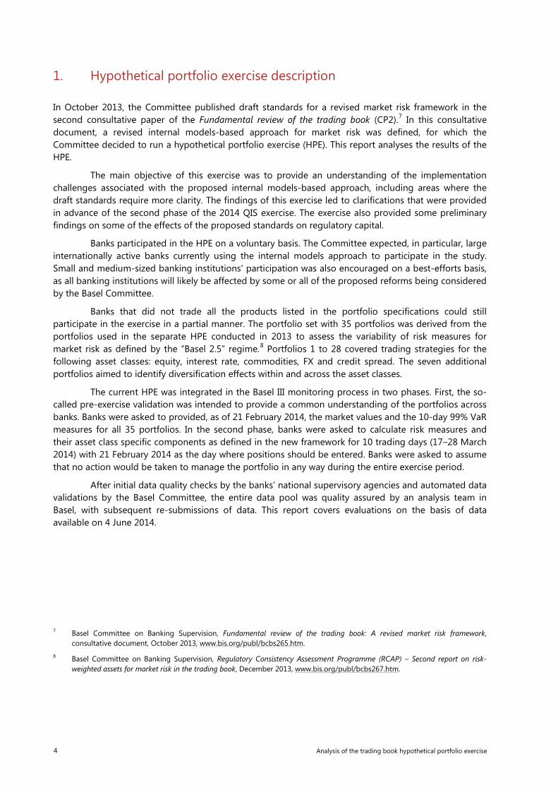
The purpose of this section is to understand how the level of constraint on diversification and hedging impacts the level of variability in the resulting risk measure. The analysis can also show how much of an impact different levels of constraint on diversification benefit can have on the overall risk measure.
For portfolio 30, using normalised data, it is clear that the variability of the liquidity-adjusted ES model results is higher when no diversification and hedging benefits across asset classes are permitted. This is consistent with what has been observed during the 2013 Regulatory Consistency Assessment Programme14, the variability of VaR and sVaR for all-in portfolios was lower than the variability observed on standalone portfolios.
This is a reasonable finding as the differences between models can compensate each other when diversification and hedging effects are not constrained. On the other hand, as this increase in the
14 See Basel Committee on Banking Supervision, Regulatory Consistency Assessment Programme (RCAP) – Second report on risk-weighted assets for market risk in the trading book, December 2013, www.bis.org/publ/bcbs267.htm.
Analysis of the trading book hypothetical portfolio exercise 11

variability of RWA is unintended, one can say that such increase in the variability is a collateral damage of the new constraint on hedging and diversification.
When diversification and hedging are fully recognised, 75% of the banks report values that are within the 50% interval around the median value. This share falls to around 70% when no diversification or hedging is recognised.
Using actual values (rather than normalised figures) we can also see how important the rho parameter is in determining both the value of the overall risk measure and its variability. For portfolio 30 as the rho parameter increases the variability reduces (once rho reaches 0.5 around 70% of the banks are within 50% of the median value) and the median value of ES reduces by 35% between its level when rho=0 and rho=1. This graph is coherent with the one before: variability decreases as more diversification and hedging are allowed.
Impact of constraining diversification and hedging
Portfolio 30 Graph 1
Expected shortfall with diversification and hedging…1 Impact of rho2 € million
1 The above data has been normalised so that the median value is 1. The vertical axis has been truncated for presentation purposes; two outliers close to 3 are not shown. 2 The vertical axis has been truncated for presentation purposes; one outlier above 15 is not shown.
Source: Basel Committee for Banking Supervision
Similar graphs showing the impact of constraining diversification and hedging for each of the diversified portfolios (portfolios 29 to 35) can be found in Appendix 1.
5.3 Analysis by asset class
The purpose of this section is to analyse the variability in the liquidity-adjusted ES measure on a portfolio by portfolio basis. To allow comparisons across portfolios, the results for each portfolio have been normalised so that the median is 1. Intuitively, greater variability for more complex products is to be expected.
5.3.1 Equity portfolios
A number of equity portfolios showed relatively high variability, in particular portfolios 5 and 6. These portfolios were the more complex of the set of equity portfolios (portfolio 5 was a variance swap, portfolio 6 a barrier option) which supports the expectation that these portfolios may have more variability. For complex products, part of the variability results from methods used to incorporate different liquidity horizons for risk factors such as spot, volatility and other. For the other portfolios, typically more than 75% of the bank results were within 50% of the median value.
12 Analysis of the trading book hypothetical portfolio exercise

5.3.2 Interest rate portfolios
In general the interest rate portfolios showed relatively low variability. With the exception of portfolio 10 (the two-year swaption, which is subject to risk factors with different liquidity horizons such as interest rates, volatility, etc) over 65% of the bank results were within 50% of the median value. For portfolio 11 approximately 90% of the banks produced results within 50% of the median.
5.3.3 FX portfolios
For the FX portfolios, all showed relatively low variability with the exception of portfolio 14 (cross-currency basis swap). Portfolio 14 appears to have a bimodal distribution, however, which could indicate that the high variability is due to different interpretations of the portfolio (ie whether exchange of notional is assumed) rather than variability of the ES measure itself.
5.3.4 Commodity portfolios
There were two commodity portfolios in the exercise. The first (portfolio 17 – gold forwards) showed low variability with over 80% of banks providing results within 50% of the median whereas the second (portfolio 18 – oil put options) showed higher variability (with less than 65% of banks reporting results within 50% of the median).
5.3.5 Credit spread portfolios
The credit spread portfolios showed the highest level of variability across all of the asset classes. The highest variability was observed in portfolios 25 and 28 where less than 50% of the participating banks provided results within 50% of the median. There is no clear link between the complexity of a portfolio and the level of variability, although the least variability was observed in portfolio 20 which was considered to be a simpler portfolio (being a sovereign bond / CDS portfolio). The CDS portfolios were designed based on market conventions. However, the contractual spreads were not specified and banks did not always make the same assumptions. The assumed spreads were supposed to be reported in a qualitative document, but they unfortunately were not always submitted to supervisors.
All related graphs can be found in Appendix 2.
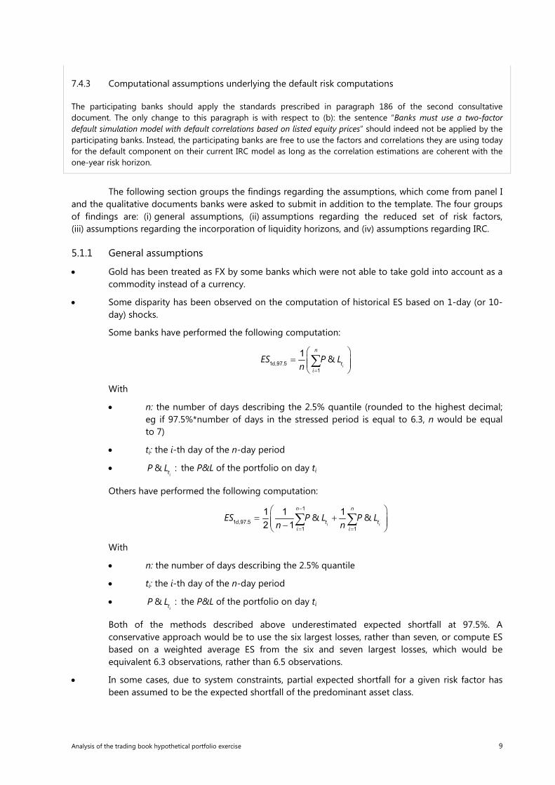
5.4 The various risk measures
The purpose of this section is to analyse the variability of the revised risk measures relative to the current ones. One could expect a higher variability of the revised measures due to the disparity in the modelling implementation (cf analysis of the replies to the closed form questions and of the qualitative documents), but also due to some features of the revised model (the ES capturing extreme events, and the longer liquidity horizons increasing the variability coming from the modelling of short horizon shocks).15
Contradictory to those assumptions, the variability (measured as the proportion of outliers) is sometimes higher, sometimes lower, whether we compare VaR/sVaR to ES, as shown in Table 3. This table has been drawn using the “strict” set of data on portfolio 30, as defined in Section 4.2, which allows a comparison of the variability of the various measures.
15 Under the mathematical assumption of normally distributed returns, the variability of VaR99% could be even larger than that of ES97.5%.
Analysis of the trading book hypothetical portfolio exercise 13

Proportion of outliers for different risk measures
In per cent Table 3
Distance to the median
10-day VaR (99%)
10-day sVaR (99%)
10-day ES (97.5%)
1-day ES (97.5%)
Liquidity-adjusted
ES (97.5%)
Revised default
risk
<75% 24 41 29 24 29 23
>125% 12 24 24 29 29 15
<50% 0 24 18 12 18 15
>150% 6 0 0 18 0 15
For portfolio 30 (the most diversified, for which we therefore expect the highest variability), three quarters of the banks were within the 50% to 150% interval,16 irrespective of the risk measure, liquidity horizon, and period of calibration.
Analysis of the various risk measures
Portfolio 30 Graph 2
Note: The above data has been normalised so that the median value is 1. The vertical axis has been truncated for presentation purposes; one outlier above 4 is not shown for three of the risk measures.
Source: Basel Committee on Banking Supervision
The same graph, computed portfolio by portfolio, can be found in Appendix 3.
It should be noted that the current IRC model (which was not analysed for this exercise) is not represented here, which limits the comparison of the variability of the current versus revised internal model treatment of default risk. Pro memoria, it has been found in previous studies that IRC models generally exhibit higher variability than VaR models.
16 ie within 50% of the median to 150% of the median.
14 Analysis of the trading book hypothetical portfolio exercise

5.5 Implementation of liquidity horizons
For the all-in-portfolio (portfolio 30) we compare the following ratios: liquidity-adjusted 97.5% ES to 10-day 97.5% ES; and liquidity-adjusted 97.5% ES to 1-day 97.5% ES.
The ratio of liquidity-adjusted 97.5% ES to 10-day 97.5% ES is in the range 1 to 3.4 with a median value of 1.5, while the ratio of liquidity-adjusted 97.5% ES to 1-day 97.5% ES is in the range 1.7 to 12.4 with a median of 4.9. The latter ratio is expected to be higher in magnitude than the former ratio, since it scales from a liquidity horizon that is 10 times larger. We can compare the two ratios by using a simplifying assumption that the 1-day ES and 10-day ES can be converted using a factor equal to the square root of 10.
Therefore, the median for the ratio of the liquidity-adjusted 97.5% ES to 10-day 97.5% ES, which is equal to 1.5, corresponds, after scaling by square root of 10, to 4.74. This figure is close to 4.9, the median for the ratio of liquidity-adjusted 97.5% ES to 1-day 97.5% ES which is equal. This comparison of the medians of the two ratios supports scaling from either a 1-day or 10-day base horizon as a viable method to arrive at the liquidity-adjusted ES, in terms of capturing data dynamics or pricing features (eg mean reversion, autocorrelation, convexity, etc).
Additionally, the range for the ratio of liquidity-adjusted 97.5% ES to 10-day 97.5% ES which is equal to 1 to 3.4 corresponds, after scaling by square root of 10 to the range 3.16 to 10.75, which spreads 7.59 and is slightly more narrow than the range for the ratio of liquidity-adjusted 97.5% ES to 1-day 97.5% ES which is 1.7 to 12.4 and spreads 10.7. The QIS HPE data therefore shows a reduction in variability of the resulting risk measure when the 10-day base horizon is used rather than 1-day method as a base horizon, albeit with significant “noise” related to these results.
For portfolio 30, moving from the current uniform liquidity horizon of 10 days to varying liquidity horizons increases the risk measure on average by 67%. It follows that for this portfolio we can imply an average revised liquidity horizon, using the square root of time scaling assumption, of 25 days. Based on the mean bank ratio of the liquidity-adjusted 97.5% ES to 1-day 97.5% ES, a revised average liquidity horizon for the all-in-portfolio equal to 30 days can also be implied. This suggests that scaling from 1 day ES may lead to a more conservative outcome.
Similarly, for the portfolios consisting of one asset class, the average revised liquidity horizon implied based on scaling from 10-day ES and 1-day ES is equal to: 18 days and respectively 8.7 days for equities;17 22 days and respectively 12 days for interest rates; 19 days and respectively 26 days for FX; 26 days and respectively 30 days commodity; and 33 days and respectively 18 days for credit. Graph 3 provides detailed results.
17 Equity portfolios are long gamma (buying options) which could explain the effect of a shorter implied liquidity horizon from 1-day ES measure.
Analysis of the trading book hypothetical portfolio exercise 15

Implementation of liquidity horizons: liquidity-adjusted ES (97.5%) divided by n-day ES (97.5%)
Portfolio 30 Graph 3
Days
Source: Basel Committee on Banking Supervision
The same graph, computed portfolio by portfolio, can be found in the Appendix 4.
16 Analysis of the trading book hypothetical portfolio exercise

Median liquidity horizon by portfolio Table 4
Portfolio number
Median liquidity horizon implied from liquidity-adjusted ES (97.5%)
divided by the 10-day ES (97.5%)
Median liquidity horizon implied from liquidity-adjusted ES (97.5%)
divided by the 1-day ES (97.5%)
1 10 8
2 10 2
3 10 6
4 10 2
5 20 8
6 11 2
7 11 4
8 18 15
9 16 5
10 16 25
11 21 13
12 20 19
13 18 40
14 15 14
15 11 19
16 20 19
17 14 10
18 27 37
19 26 41
20 18 13
21 45 40
22 56 45
23 39 27
24 62 64
25 32 14
26 21 11
27 38 28
28 20 12
29 28 33
30 21 24
31 17 8
32 21 10
33 18 26
34 24 28
35 38 10
5.6 Share of the three risk measures (ES, NMRF and IDR) in the total
This section analyses the share of the three risk measures under the revised framework: the ES, the losses from NMRFs, and the IDR.
Analysis of the trading book hypothetical portfolio exercise 17

The parameters have been set as follows: The parameter constraining diversification and hedging benefits, ρ, has been set to 0.5, while the multiplier (which applies to both ES and NMRF) has been set to 3. Each measure is computed as the simple sum of the measures reported by the banks which have been able to report ES, NMRF and IDR. Data is then represented as a percentage of the total sum of the three measures.
As Graph 4 shows, the share of IDR is relatively low and that of NMRF even lower. Besides the credit spread asset class, IDR and NRMF are negligible in comparison to ES. Nevertheless, this result is limited by the fact that several banks faced difficulties in implementing the NMRF framework, and in expanding the IDR to equities.
Graph 4 shows that the share of IDR is limited for portfolios 1 to 7, which are the equity portfolios. On the other hand, it also shows that at least some banks have been able to adapt their IRC model. The share for which NMRF represent in the total can go as high as 8% for portfolio 28.
Share of the three risk measures (ES, NMRF and IDR) in the total
All portfolios Graph 4
Per cent
Source: Basel Committee on Banking Supervision
The same graph, computed asset class by asset class, can be found in the Appendix 5.
5.7 New risk measure compared with the current one
The comparison between the proposed ES risk measure and the current 10-day VaR method was performed based on the ratio:
( )( )
EQ IR FX Comm CSS S S S SES ES ES ES ES ES
VaR StressedVaRρ ρ+ − + + + +
+1
with ρ = 0.5 set to control the amount of hedging and diversification benefit that is recognised
across asset classes, where FCRS
RC
ESES ES
ES= .
The new risk measure consists of: changes that we expect would reduce capital (eg the use of a single risk measure at a lower confidence level); and changes that would increase capital (eg averaging in the tail of the distribution, longer liquidity horizons, and less diversification recognised across asset classes). The resulting effect for portfolio 30 is that the risk measure increases by 80% for the mean bank. For the mean bank in all asset classes there is an increase in the risk measure, with the exception of equities where the risk measure decreases by 9%.
18 Analysis of the trading book hypothetical portfolio exercise

Ratio of capital requirements implied by new and old frameworks Graph 5
The vertical axis has been truncated for presentation purposes; one outlier above 6 is not shown for portfolio 22.
Source: Basel Committee on Banking Supervision
5.8 Variance of each variable through time
The analysis included in this report has largely been based on risk measure data for the final date of the QIS period. This approach is valid provided each risk measure remains relatively stable over the whole QIS period (which ensures taking a single data point will be representative).
For the HPE all of the risk measure time series were broadly stable over the 10-day period, for example for the ES measure the standard deviation was typically less than 5% of the mean of the time series, with only portfolios 2 and 6 showing higher variability (where the standard deviation of the time series was 34% and 11% respectively of the mean).
5.9 Closed form questions
5.9.1 Question 1
Question 1 asked: “How many trading desks (as defined in the second consultative document) do you have?” This question was designed to collect information on the number of desks banks consider defining for the coming QIS. The answers received are summarised in Table 5.
Number of respondents to each possible answer to question 1 Table 5
Number of respondents Per cent of respondents
Between 1 and 20 19 50.0
Between 20 and 50 10 26.3
Between 50 and 100 7 18.4
Between 100 and 150 1 2.6
Above 150 1 2.6
From this table, the following conclusions can be drawn:
• Half of the respondents have between one and 20 desks.
• 76.3% of the respondents have less than 50 desks.
• Only two banks have reported more than 100 desks.
Analysis of the trading book hypothetical portfolio exercise 19

5.9.2 Question 2
Question 2 asked: “Based on your internal risk assessment, how well spread is risk across your trading desks? In order to assess this, take your 10% most material trading desks (ie if you have 100 desks, take the 10 desks which have the highest standalone risk – as measured, for instance, by a VaR number), and compute the ratio of the sum of the standalone risks from these desks divided by the overall risk (sum of all standalone risks across all desks). Is this ratio greater than:”.
The question was designed to assess the degree of concentration of the risks within the largest 10% of the desks of a bank. The answers received are summarised in Table 6.
Number of respondents to each possible answer to question 2 Table 6
Number of respondents Per cent of respondents
> 10% 1 100.0
> 20% 3 97.1
> 30% 11 88.6
> 40% 11 57.1
> 50% 3 25.7
> 60% 2 17.1
> 70% 4 11.4
> 80% 0 0.0
From this table, the following conclusions can be drawn:
• For only ¼ of the banks, the 10% of the largest desks account for more than 50% of the risks.
• For the remaining ¾ of the banks, they account for between 10 and 50% of the risks.
• For 88.6% of the respondents, the 10% of the largest desks take more than 30% of the risks.
• For 57.1% of the respondents, the 10% of the largest desks take more than 40% of the risks.
The degree of concentration of risks within the main desks of a bank is therefore very high.
5.9.3 Questions 3 and 4
Question 3 asked: “In addition to the idiosyncratic factor, does your current IRC model take into account the following systematic factors? Please state the number of characteristics which are possible for the individual risk factor (0 if the factor is not included in your model). If you use factors different from global, industry and region, please state the number of possible characteristics each factor could take in sub-questions Q4 to Q6.”
This question was designed to gather information regarding the risk factors banks use in their current IRC models. This information should be useful in order to further determinate whether or not the requirement for a two-factor model should be kept, deleted, or further specified. The responses received are summarised in Table 7.
20 Analysis of the trading book hypothetical portfolio exercise

Number of respondents to each possible answer to question 3 Table 7
Number of respondents Per cent of respondents
Only idiosyncratic 6 22.2
Idiosyncratic & global 5 29.6
Idiosyncratic & industrial 2
Idiosyncratic & region 0
Idiosyncratic & additional 1
Idiosyncratic & two others amongst the global industry and region 5 22.2
Idiosyncratic & two others (one amongst the global industry and region and one amongst the additional
1
Idiosyncratic & two others amongst the global industry and region plus one amongst the additional
0 22.2
Idiosyncratic & global industry and region 6
Idiosyncratic & global industry and region and additional 1 3.7
51.9 percent of the respondents have either only the idiosyncratic factor, or this factor plus another one. Yet, there is some dispersion between which factors are used. Then 22.2 percent of the banks have a so-called two-factor model (defined as two factors in addition to the idiosyncratic factor). 25.9 percent of the banks have an IRC more sophisticated than a two-factor model (ie they have a three- or more factor model).
Question 4 asked: “What type of data do you use to calculate correlations which are used in your IDR model?”. The answers received are summarised in Table 8.
Number of respondents to each possible answer to question 4 Table 8
Number of respondents Per cent of respondents
Equity data only 8 34.8
CDS data only 3 13.0
Mix of equity and CDS data 2 8.7
Mix of equity and other data 4 17.4
Mix of CDS and other data 4 17.4
Mix of equity CDS and other data 2 8.7
Equity data no CDS data 52.2
CDS data no equity data 30.4
Equity data and CDS data 17.4
Banks tended to use more frequently equity data than CDS data in their IDR. Only 17.4 precent of them use both.
5.9.4 Question 5
Question 5 asked: “When implementing the varying liquidity horizon, did you apply?”. The intention of the question was to understand the most popular approach used in the exercise to integrate varying liquidity horizons to the internal model. The answers received are summarised in Table 9.
Analysis of the trading book hypothetical portfolio exercise 21

Number of respondents to each possible answer to question 5 Table 9
Number of respondents Per cent of respondents
bcbs265 approach 29 76.3
ISDA/GFMA/IIF - Joint response variant 1 1 2.6
ISDA/GFMA/IIF - Joint response variant 2 1 2.6
ISDA/GFMA/IIF - Joint response variant 3 2 5.3
Any other variant 5 13.2
The responses show that the approach defined in CP2 was the most widely used one in the exercise, and the ISDA/GFMA/IIF variants were only used by 10.5 percent of the participating banks. This appears to indicate that the CP2 approach can be implemented (at least in the case of a small number of hypothetical portfolios).
5.9.5 Questions 6 and 7
Questions 6 and 7 were closely related. Question 6 asked: “When computing the current value-at-risk for interest rate risks, do you use market rates or zero coupon rates?” For those banks who indicated they used market rates, question 7 requested further information: “If you use market rates for your current value-at-risk, does it mean your IT system does not allow you to compute zero coupon rates?”
The intention of the questions was to better understand the practice of banks when considering interest rate risk and the feasibility of requiring the use of zero coupon rates. The responses to question 6 are summarised in Table 10.
Number of respondents to each possible answer to question 6 Table 10
Number of respondents Per cent of respondents
Market rates 9 23.1
Zero coupon rates 22 56.4
Either market rates or zero coupon rates depending on product 8 20.5
The responses show a relatively even split between banks who only use zero coupon rates and those who either only use market rates or use market rates for at least some products. For the 19 banks that always use market rates or use them for some products the responses to question 7 are summarised in Table 11.
Number of respondents to each possible answer to question 7 Table 11
Number of respondents Per cent of respondents
Yes it does not allow it at all 0 0.0
No it does allow it but it is demanding 11 64.7
No it does allow it easily 6 35.3
From these responses it is clear that in all cases it is at least possible for zero coupon rates to be used, although for the majority of banks who do not use them exclusively at the moment it is demanding for current IT systems to do so.
5.9.6 Question 8
Question 8 asked: “Regarding the frequency of your data input updates, what is the lowest frequency of update across all your modellable risk factors?” The question was designed to better understand how
22 Analysis of the trading book hypothetical portfolio exercise

regularly data is updated, and whether the frequency varied across banks. The responses are summarised in Table 12.
Number of respondents to each possible answer to question 8 Table 12
Number of respondents Per cent of respondents
Daily 23 59.0
Weekly 2 5.1
Bi-weekly 5 12.8
Monthly 7 17.9
Quarterly 1 2.6
More than quarterly 1 2.6
The majority of banks indicate that they have daily updates to their input data, however there is a wide range of practice across banks with over one third updating their data only on a bi-weekly or longer basis.
5.10 Approval status
The majority of data provided by banks was based on regulatory approved models. For the ES model on average across all portfolios, 84% of the models used were regulatory approved. For the IDR model, on average across all portfolios, 56% of the models used were regulatory approved. Detailed results by portfolio are presented in Table 13.
Analysis of the trading book hypothetical portfolio exercise 23

Approval status Table 13
Regulatory Management
Portfolio number ES IDR1 ES IDR1
1 28 7 4 3
2 25 6 5 4
3 26 6 6 3
4 24 6 5 3
5 19 6 4 2
6 22 6 4 2
7 19 6 5 2
8 32 13 6 5
9 34 0 5 0
10 32 0 3 0
11 20 0 5 0
12 23 0 2 0
13 33 0 6 0
14 33 0 3 0
15 30 0 5 0
16 26 0 6 0
17 27 0 6 0
18 24 0 4 0
19 25 16 5 4
20 24 15 6 5
21 23 17 4 4
22 26 16 4 5
23 22 16 4 4
24 22 16 4 4
25 21 15 4 4
26 22 15 4 4
27 12 9 5 3
28 15 11 3 2
29 24 11 8 6
30 25 11 8 6
31 24 8 6 3
32 30 11 5 6
33 31 6 4 5
34 24 6 5 3
35 24 13 6 5 1 Portfolios 9 to 18 are interest rate, FX, and commodity portfolios, which explains why no IDR has been computed for them.
24 Analysis of the trading book hypothetical portfolio exercise

5.11 Stressed period
Banks’ choice of stressed period was broadly consistent, with most banks choosing periods that overlapped with the second half of 2008. Only five banks selected stressed periods that did not at least include Q4 2008.
It is interesting to observe that even banks located in non-US and non-EU countries all have their stressed period in 2008. In no country a more stressed period was found, even in those countries which used to be more strongly hit in crises occurring before the recent financial crisis.
Stressed period Graph 6
Graph shows the number of banks whose stressed period includes the quarter.
Source: Basel Committee on Banking Supervision
6. Conclusions
The second consultative document for the fundamental review of the trading book proposed significant changes to the current market risk framework. The hypothetical portfolio exercise on the Internal Models Approach provided encouraging results supporting the new framework. Over 40 banks from various jurisdictions were able to implement the requirements for internal models given some simplifying assumptions. Banks were able to leverage the existing risk systems and perform the computation for the new risk measures within two quarters of the publication of the consultative document. The exercise provided valuable information that will be used to refine the instructions for the subsequent QIS’ on actual bank portfolios. Based on the results of the hypothetical portfolio exercise assessed in this report, the new risk measures proposed in the second consultative document are not likely to increase variability in comparison to the measures in the current market risk framework.
Analysis of the trading book hypothetical portfolio exercise 25

Appendix 1: Impact of constraining diversification and hedging
Impact of constraining diversification and hedging
In millions of euros Graph 7
Portfolio 29 I Portfolio 30
Portfolio 31 Portfolio 32
Portfolio 33 Portfolio 34
26 Analysis of the trading book hypothetical portfolio exercise
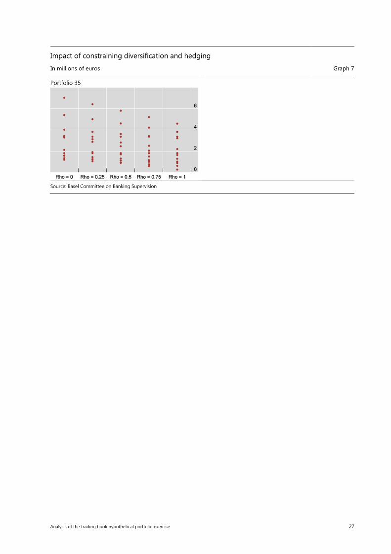
Impact of constraining diversification and hedging
In millions of euros Graph 7
Portfolio 35
Source: Basel Committee on Banking Supervision
Analysis of the trading book hypothetical portfolio exercise 27

Appendix 2: Analysis by asset class.
Analysis by asset class Graph 8
Equity portfolios Interest rate portfolios Liquidity-adjusted ES normalised by the median Liquidity-adjusted ES normalised by the median
FX portfolios Commodity portfolios
Liquidity-adjusted ES normalised by the median Liquidity-adjusted ES normalised by the median
Credit spread portfolios
Liquidity-adjusted ES normalised by the median
Note: The above data has been normalised so that the median value is 1.
Source: Basel Committee on Banking Supervision
28 Analysis of the trading book hypothetical portfolio exercise

Appendix 3: Analysis of the various risk measures
Analysis of the various risk measures Graph 9
Portfolio 1
Portfolio 2
Portfolio 3
Analysis of the trading book hypothetical portfolio exercise 29

Analysis of the various risk measures Graph 9
Portfolio 4
Portfolio 5
Portfolio 6
Portfolio 7
30 Analysis of the trading book hypothetical portfolio exercise

Analysis of the various risk measures Graph 9
Portfolio 8
Portfolio 9
Portfolio 10
Portfolio 11
Analysis of the trading book hypothetical portfolio exercise 31

Analysis of the various risk measures Graph 9
Portfolio 12
Portfolio 13
Portfolio 14
Portfolio 15
32 Analysis of the trading book hypothetical portfolio exercise

Analysis of the various risk measures Graph 9
Portfolio 16
Portfolio 17
Portfolio 18
Portfolio 19
Analysis of the trading book hypothetical portfolio exercise 33

Analysis of the various risk measures Graph 9
Portfolio 20
Portfolio 21
Portfolio 22
Portfolio 23
34 Analysis of the trading book hypothetical portfolio exercise

Analysis of the various risk measures Graph 9
Portfolio 24
Portfolio 25
Portfolio 26
Portfolio 27
Analysis of the trading book hypothetical portfolio exercise 35
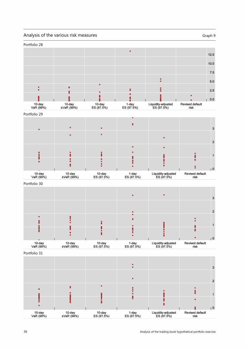
Analysis of the various risk measures Graph 9
Portfolio 28
Portfolio 29
Portfolio 30
Portfolio 31
36 Analysis of the trading book hypothetical portfolio exercise

Analysis of the various risk measures Graph 9
Portfolio 32
Portfolio 33
Portfolio 34
Analysis of the trading book hypothetical portfolio exercise 37

Analysis of the various risk measures Graph 9
Portfolio 35
Note: The above data has been normalised so that the median value is 1.
Source: Basel Committee on Banking Supervision
38 Analysis of the trading book hypothetical portfolio exercise

Appendix 4: Implementation of liquidity horizons
Liquidity-adjusted ES (97.5%) divided by n-day ES (97.5%) Graph 10
Portfolio 1 Portfolio 2 Portfolio 3 Portfolio 4
Portfolio 5 Portfolio 6 Portfolio 7 Portfolio 8
Portfolio 9 Portfolio 10 Portfolio 11 Portfolio 12
Analysis of the trading book hypothetical portfolio exercise 39

Liquidity-adjusted ES (97.5%) divided by n-day ES (97.5%) Graph 10
Portfolio 13 Portfolio 14 Portfolio 15 Portfolio 16
Portfolio 17 Portfolio 18 Portfolio 19 Portfolio 20
Portfolio 21 Portfolio 22 Portfolio 23 Portfolio 24
Portfolio 25 Portfolio 26 Portfolio 27 Portfolio 28
40 Analysis of the trading book hypothetical portfolio exercise

Liquidity-adjusted ES (97.5%) divided by n-day ES (97.5%) Graph 10
Portfolio 29 Portfolio 30 Portfolio 31 Portfolio 32
Portfolio 33 Portfolio 34 Portfolio 35
Source: Basel Committee on Banking Supervision
Analysis of the trading book hypothetical portfolio exercise 41

Appendix 5: Share of the three risk measures
Share of the three risk measures (ES, NMRF and IDR) in the total Graph 11
All portfolios Per cent
Equity portfolios Interest rate portfolios FX portfolios
Per cent Per cent Per cent
Commodity portfolios Credit spread portfolios All-in portfolios
Per cent Per cent Per cent
Source: Basel Committee on Banking Supervision
42 Analysis of the trading book hypothetical portfolio exercise
Appendix 6: Portfolio specification for the Hypothetical Portfolio Exercise
Computational assumptions
Banks should calculate the risks of the positions without taking into account the funding costs associated to the portfolios (ie no assumptions are admitted as per the funding means of the portfolios).
Banks should exclude to the extent possible counterparty credit risk when valuing the risks of the portfolios.
For transactions that include long positions in CDS, assume an immediate up-front fee is paid to enter the position as per the market conventions as indicated by Markit Partners (25, 50, 100bps for investment grade, 500bps for high yield).
Assume that the maturity date for all CDS in the exercise follow conventional quarterly termination dates, often referred to as “IMM dates”.
Additional specifications required in order to compute pricing calculations required for CDS positions should be done in a way that is consistent with commonly used market standards.
Use the maturity date (ie some options expire on third Saturday of the month, etc) that ensures the deal is closest to the term-to-maturity specified. For any material details of the product specification that are not explicitly stated in this document, please provide the assumptions you have used along with the results (ie day count convention, etc).
The acronyms ATM, OTM and ITM refer to an option’s moneyness: ATM stands for “at the money”, OTM stands for “out of the money”, and ITM means “in the money”.
Assume that all options are traded over-the-counter unless explicitly specified in the portfolios
Follow the standard timing conventions for OTC options (ie expiry dates are the business day following a holiday).
Assume that the timing convention for options is as follows: The time to maturity for a n-month option entered on 21 February is in n months. For example, a 3-month OTC option entered on 21 February 2014 expires on 21 May 2014. If options expire on a non-trading day, adjust the expiration date as per business day conventions consistent with common practices. Also provide explicit details on the nature of the adjustment made.
Assume that the exercise style for all OTC options specified is as follows:
• American for single name equities and commodities; and
• European for equity indices, foreign exchange and swaptions.
For all options exclude the premium from the initial market value calculations (ie options are to be considered as “naked”).
In the case that a bank is required to make additional assumptions beyond those specified above that it believes are relevant to the interpretation of its exercise results (eg close of business timing, coupon rolls, mapping against indices, etc), it should submit a description of those specifications in a separate document accompanying its return template.
Analysis of the trading book hypothetical portfolio exercise 43

1. Portfolio definition
Portfolio number Risk factor
Strategy
Equity portfolios
1 Equity
Equity index futures Long delta • Long 30 contracts ATM 3-month front running FTSE 100 index futures * Futures price is based on the index level at NYSE Liffe London market close on 21 February 2014. 1 contract corresponds to 10 equities underlying.
2 Equity
Bullish leveraged trade Long gamma and long vega • Long 100 contracts OTC Google (GOOG) OTM 3-month call options (1 contract = 100 shares
underlying) * Strike price is out-of-the-money by 10% relative to the stock price at market close on 21 February 2014.
3 Equity
Volatility trade #1 Short short-term vega & long long-term vega • Short straddle 3-month ATM* S&P 500 Index OTC options (30 contracts) • Long straddle 2-year ATM S&P 500 Index OTC options (30 contracts) 1 contract corresponds to 100 equities underlying effective date 21 February 2014 * Strike price is based on the index level at NYSE at 4.30 pm New York on 21 February 2014.
4 Equity
Volatility trade #2 (smile effect) Long/short puts on FTSE 100 • Long 40 contracts of 3-month put options on FTSE 100 index (with a strike price that is 10%
OTM* based on the end-of-day index value) • Short 40 contracts of 3-month put options on FTSE 100 index (with a strike price that is 10%
ITM* based on the end-of-day index value) * Strike price is based on the index level at NYSE Liffe London market close on 21 February 2014. 1 contract corresponds to 10 equities underlying.
5 Equity
Equity variance swaps on Eurostoxx 50 (SX5E) • Long ATM variance swap on Eurostoxx 50 with a maturity of 2 years, Vega notional amount
of €50,000. The payoff is based on the following realised variance formula:
[ln( )]n
i
i i
Sn S
−+
=− ∑1
21
1
2522
where n = number of working days until maturity. The strike of the variance swap should be defined on the trade date (21 February 2014) to cancel the value of the swap. (Please provide the strike you determined on the pre-exercise validation data template together with the initial market value of the trade.)
6 Equity
Barrier option • Long 40 contracts of 3-month ATM* S&P 500 down-and-in put options with a barrier level
that is 10% OTM* and continuous (monitoring frequency. 1 contract corresponds to 100 equities underlying * Strike price is based on the index level at NYSE market close on 21 February 2014.
7 Equity
Quanto index call • 3-year USD Quanto call on Eurostoxx 50 See details in Section 2.1 of this Annex.
44 Analysis of the trading book hypothetical portfolio exercise

Portfolio number Risk factor
Strategy
Interest rate
8 Interest rate
Curve flattener trade Long long-term and short short-term treasuries • Long €5 million 10-year German Treasury bond (ISIN: DE0001102333, expiry 15 February
2024) • Short €20 million 2-year German Treasury note (ISIN: DE0001135291, expiry 4 January 2016)
9 Interest rate
Interest rate swap Bloomberg code eusw10v3 curncy • Receive fixed rate and pay floating rate • Fixed leg: pay annually • Floating leg: 3-month Euribor rate, pay quarterly • Notional: €5 million • Roll convention and calendar: standard • Effective date 21 February 2014 (ie rates to be used are those at the market as 21 February
2014) • Maturity date: 21 February 2024
10 Interest rate
Two-year swaption on 10-year interest rate swap Bloomberg code eusv0210 curncy • An OTC ATM* receiver swaption with maturity of two years on the interest rate swap
described in #9 (ie ten years fixed for variable IRS) but with an effective date of 22 February 2016 and a maturity date of 22 February 2026.
• effective date 24 February 2016 • expiry date (of swaption) 22 February 2016 • maturity date (of underlying swap) 24 February 2026 • premium paid at expiry • cash settled * strike price is based on the IRS rate as per #9 (ie the strike price is the fixed rate as per #9)
11 Interest rate
LIBOR range accrual Structured coupon indexed on the number of days in the interest rate period when the Libor fixes in a predetermined range. See details in Section 2.2 of this Annex.
12 Interest rate
Inflation zero coupon swap EURHICPX index 10Y maturity par zero coupon swap See details in Section 2.3 of this Annex.
FX
13 FX
Covered FX call Short EUR/USD and short put EUR call USD option • Short 3-month EUR/USD forward contracts (ie long USD short EUR) with USD 20 million
notional purchased at the EUR/USD ECB reference rate as of end of day 21 February 2014 • Short 3-month put EUR call USD option notional USD 40 million (ie short USD against EUR)
with strike price corresponding to the three-month forward exchange rate as of end of day 21 February 2014
• effective date 21 February 2014 • expiry date 21 May 2014
14 FX
Mark-to-market cross-currency basis swap 2 Year USD 3M LIBOR vs EUR 3M EURIBOR swap See details in Section 2.8 of this Annex.
Analysis of the trading book hypothetical portfolio exercise 45

Portfolio number Risk factor
Strategy
15 FX
Knock-out option Vanilla option that ceases to exist if the underlying spot breaches a predetermined barrier before maturity See details in Section 2.4 of this Annex.
16 FX
Double no touch option Digital option that pays a predetermined amount if the spot does not touch any of the barriers during the life of the option See details in Section 2.5 of this Annex.
Commodity
17 Commodity
Curve play from contango to backwardation Long short-term and Short long-term contracts • Long 3,500,000 3-month ATM OTC London Gold Forwards contracts (1 contract = 0.001 troy
ounces, notional: 3,500 troy ounces) • Short 4,300,000 1-year ATM OTC London Gold Forwards contracts (Notional: 4,300 troy
ounces)
18 Commodity
Short oil put options • Short 30 contracts (U4 Sep.) of 3-month OTC WTI Crude Oil puts with strike = 6-month end-
of-day forward price on 21 February 2014 (1 contract = 1000 barrels, total notional 30,000 barrels)
Credit spread
19 Credit spread
Sovereign CDS portfolio Short protection via CDS on five countries • Short €2 million per single-name 5year CDS (total 10 million notional) on the following
countries: • effective date: 21 February 2014 • restructuring clause: FULL
Country RED Code currency
Italy 4AB951 USD
UK 9A17DE USD
Germany 3AB549 USD
France 3I68EE USD
US 9A3AAA EUR
46 Analysis of the trading book hypothetical portfolio exercise

Portfolio number Risk factor
Strategy
20 Credit spread
Sovereign bond/CDS portfolio Long protection via CDS on five countries • Long €2 million per single-name 5 year CDS (total 10 million notional) on the following
countries: Italy, UK, Germany, France, US as in portfolio #19. • Long €2 million per single-name 5 year bonds (total 10 million notional) on the following
countries: Italy, UK, Germany, France, US (as identified in the following table) • effective date 21 February 2014 • to convert the notional of the non-euro bonds use the FX spot as at end of day 21 February
2014
Identifier Description
IT0003493258 BTP 1 February 2019
DE0001135374 BUND 4 January 2019
GB00B39R3F84 GILT 7 March 2019
FR0000189151 OAT 25 April 2019
US912828SH49 TBOND 28 February 2019
21 Credit spread
Sector concentration portfolio Short protection via CDS on 10 financials • Equivalent of short 1 million notional per single-name 5 year CDS (total €10 million notional)
on the following 10 companies • effective date 21 February 2014
Name RED Code Currency Doc clause
Met Life 5EA6BX USD MR
Allianz DD359M EUR MM
Prudential 7B8752 USD MR
AXA FF667M EUR MM
ING BANK 48DGFE EUR MM
Aegon 007GB6 EUR MM
Aviva GG6EBT EUR MM
Swiss Re HOB65N EUR MM
Principal Financial Group 7B676W USD MR
Suncorp Group 8ED955 USD MR
22 Credit spread
Diversified index portfolio Short protection via CDS index • Short €10 million notional iTraxx 5-year Europe index Series 20, Version 1 – maturity
20 December 2018 (RED Pair Code: 2I666VBA2) • effective date 21 February 2014
Analysis of the trading book hypothetical portfolio exercise 47

Portfolio number Risk factor
Strategy
23 Credit spread
Diversified index portfolio (higher concentration) Short protection via CDS index • Short €5 million notional iTraxx 5-year Europe index Series 20, Version 1 – Maturity
20 December 2018 (RED Pair Code: 2I666VBA2) • Short €5 million notional (equally weighted = €1 million for each CDS) on the following five
financials belonging to the iTraxx 5-year Europe index Series 20, Version 1 – Maturity 20 December 2018 (RED Pair Code: 2I666VBA2):
CDS name RED Code Currency Doc clause
ING BK CDS EUR SR 5Y 48DGFEAH6 EUR MM
CMZB CDS EUR SR 5Y 2C27EGAG9 EUR MM
AXA SA CDS EUR SR 5Y FF667MAD8 EUR MM
AEGON CDS EUR SR 5Y 007GB6AD4 EUR MM
SANTAN CDS EUR SR 5Y EFAGG9AF6 EUR MM
• Effective date: 21 February 2014.
24 Credit spread
Diversified corporate portfolio Short protection via CDS on 10 A- to AA- corporate • Short equivalent of €2 million notional per single-name 5 year CDS (total €20 notional) on
the following 10 companies (for USD CDS use the exchange rate at 21 February 2014):
Name RED Code Currency Doc clause
P&G 7B6989 USD MR
Home Depot 47A77D USD MR
Siemens 8A87AG EUR MM
Royal Dutch Shell GNDF9A EUR MM
IBM 49EB20 USD MR
Met Life 5EA6BX USD MR
Southern Co 8C67DF USD MR
Vodafone 9BADC3 EUR MM
BHP 08GE66 USD MR
Roche 7E82AF EUR MM
25 Credit spread
Index basis • Short €5 million notional iTraxx 5-year Europe index Series 20, Version 1 – Maturity
20 December 2018 (RED Pair Code: 2I666VBA2) • Effective date: 21 February 2014 • Long €5 million notional on all constituents of iTraxx 5-year Europe index Series 20, Version
1 – maturity 20 December 2018 (RED Pair Code: 2I666VBA2) (ie the aggregate notional is €5 million and all names are equally weighted); convention: 100 bp running coupon
• Effective date: 21 February 2014
48 Analysis of the trading book hypothetical portfolio exercise

Portfolio number Risk factor
Strategy
26 Credit spread
CDS bond basis • Long bonds €2 million per single-name 5 year bonds on 5 Financials (3 EU, 2 North
America).
ISIN Security name
XS0834640541 MET LIFE GLOB FUNDING I 30 September 2019
XS0406076843 ALLIANZ SE 18 December 2018
US74432QBG91 PRUDENTIAL FINANCIAL INC 15 June 2019
FR0011322668 AXA SA 20 September 2019
DE000A1HNFX5 ING BANK NV 15 February 2019
• Long protection via CDS on the same names (€2 million per single-name 5 year).
Name RED Code Currency Doc clause
Met Life 5EA6BX USD MR
Allianz DD359M EUR MM
Prudential 7B8752 USD MR
AXA FF667M EUR MM
ING 49BEBA EUR MM
27 Credit spread
Short index put on ITraxx Europe Crossover series 20 See details in Section 2.6 of this Annex.
28 Credit spread
Quanto CDS on Spain with delta hedge See details in Section 2.7 of this Annex.
All-in portfolios
29 All-in portfolio (1) All portfolios excluding portfolios 5, 7, 11, 12, 15, 16, 27, 28.
30 All-in portfolio (2) All portfolios
31 All-in portfolio (3) All equity portfolios (ie comprising portfolios from #1 to #7)
32 All-in portfolio (4) All interest rate portfolios (ie comprising portfolios from #8 to #12)
33 All-in portfolio (5) All FX portfolios (ie comprising portfolios from #13 to #16)
34 All-in portfolio (6) All commodity portfolios (ie comprising portfolios from #17 to #18)
35 All-in portfolio (7) All credit spread portfolios (ie comprising portfolios from #19 to #28)
Analysis of the trading book hypothetical portfolio exercise 49

2. Details for portfolios
2.1 Details for portfolio 7: 3-year USD quanto call on EUROSTOXX 50
Party A: counterparty
Party B: participating bank
Equity Notional Amount (ENA): USD 5,000,000
Trade date: 21 February 2014
Strike date: 21 February 2014
Effective date: 21 February 2014
Valuation date: ` 21 February 2017
Termination date: 21 February 2017
Underlying index: EURO STOXX 50 (Bloomberg: SX5E Index)
Floating rate payer: Counterparty
Notional amount: USD 5,000,000
Floating rate: USDLIBOR3M as determined at 11.00am London time two (2) business days prior to the start of the relevant interest period
Spread: + 300 bps
Floating rate day count fraction: act/360
n/floating amount payment dates: 1/ 21 May 2014
2/ 21 August 2014
3/ 21 November 2014
4/ 20 February 2015
5/ 21 May 2015
6/ 21 August 2015
7/ 20 November 2015
8/ 22 February 2016
9/ 20 May 2016
10/ 22 August 2016
11/ 21 November 2016
12/ 21 February 2017
Equity amount payer: participating bank
Equity amount: On the termination date, Party B will pay Party A the following cash settlement amount:
50 Analysis of the trading book hypothetical portfolio exercise

max %, Final Initial
Initial
Index IndexENA
Index −
× 0
Where
IndexInitial is the official closing level of the underlying index on the strike date.
IndexFinal is the official closing level of the underlying index on the valuation date.
Settlement terms:
Settlement currency: USD Quanto
Business days: New York
Analysis of the trading book hypothetical portfolio exercise 51

2.2 Details for portfolio 11: 3M Libor USD range accrual
Party A Participating bank
Party B Counterparty
Notional amount USD 10,000,000.0
Trade date: 21 February 2014
Effective date: 21 February 2014
Termination date: 21 February 2024
Party A pays: 4% *n/N
n: Number of days when the range accrual index fixes between the lower barrier and the upper barrier (inclusive) during the relevant interest period
N: Number of days in the relevant interest period
Range accrual index: 3-month USD Libor as quoted on Reuters page LIBOR01, 11:00 London Time
USD 3M Libor: 3-month USD Libor as quoted on Reuters page LIBOR01, 11:00 London time, fixed 2 business days prior to the first day of each interest period
Lower barrier: 2.50%
Upper barrier: 4.00%
Day count fraction: Actual/360
Payment dates: Quarterly
Business day convention: Modified Following
Business days for fixing: London and New York
Business days for payment: London and New York
Party B pays: USD 3M Libor
USD 3M Libor: 3-month USD Libor as quoted on Reuters page LIBOR01, 11:00 London time, fixed 2 business days prior to the first day of each interest period
Day count fraction: Actual/360
Payment dates: Quarterly
Business day convention: Modified Following
Business days for fixing: London and New York
52 Analysis of the trading book hypothetical portfolio exercise

Business days for payment: London and New York
Interest period: From the previous payment date (inclusive) to the next payment date (exclusive)
Analysis of the trading book hypothetical portfolio exercise 53

2.3 Details for portfolio 12: EURHICPX index 10Y maturity zero coupon swap
Contract date: 21 February 2014
Payer of fixed: participating bank
Payer of HICP XT Float: counterparty
Notional amount: EUR 10,000,000.00
Start date: 21 February 2014
Maturity date: 21 February 2024
Fixed rate details
Fixed rate 2.000 per cent
Payment day convention Modified Following
Payment days Target
Fixed payment dates 21 February 2024
HICP XT Float rate details
Float rate Target
Frequency At maturity in arrears
Index name Eurostat Eurozone HICP Ex Tobacco Unrevised Series NSA
Payment days 21 February 2024
HICP XT Fixed rate calculation method
Notional amount*[((1+Fixed rate)^n)-1]
HICP XT Floating rate calculation method Notional amount*[Index(end)/Index(start)-1]
Index (end) = HICP XT Nov 2023 Index unrevised
Index (start) = HICP XT Nov 2013 Index unrevised
There is no floor.
54 Analysis of the trading book hypothetical portfolio exercise
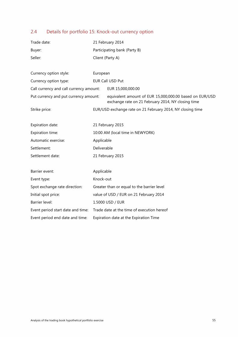
2.4 Details for portfolio 15: Knock-out currency option
Trade date: 21 February 2014
Buyer: Participating bank (Party B)
Seller: Client (Party A)
Currency option style: European
Currency option type: EUR Call USD Put
Call currency and call currency amount: EUR 15,000,000.00
Put currency and put currency amount: equivalent amount of EUR 15,000,000.00 based on EUR/USD exchange rate on 21 February 2014, NY closing time
Strike price: EUR/USD exchange rate on 21 February 2014, NY closing time
Expiration date: 21 February 2015
Expiration time: 10:00 AM (local time in NEWYORK)
Automatic exercise: Applicable
Settlement: Deliverable
Settlement date: 21 February 2015
Barrier event: Applicable
Event type: Knock-out
Spot exchange rate direction: Greater than or equal to the barrier level
Initial spot price: value of USD / EUR on 21 February 2014
Barrier level: 1.5000 USD / EUR
Event period start date and time: Trade date at the time of execution hereof
Event period end date and time: Expiration date at the Expiration Time
Analysis of the trading book hypothetical portfolio exercise 55

2.5 Details for portfolio 16: Double no touch binary currency option
Trade Date: 21 February 2014
Buyer: participating bank (Party B)
Seller: Client [Party A]
Currency option style: Binary
Expiration date: 21 February 2015
Expiration time: 10:00 am (local time in New York)
Automatic exercise: Applicable
Settlement: Non-deliverable
Settlement amount: EUR 1, 000,000.00
Settlement date: 21 February 2015
Barrier event: Applicable
Event type: Double No-Touch Binary
Initial spot price: level of USD/EUR on 21 February 2014
Upper barrier level: 1.5000 USD / EUR
Lower barrier level: 1.2000 USD / EUR
Event period start date and time: Trade date at the time of execution hereof
Event period end date and time: Expiration date at the expiration time
Business day convention: Following
56 Analysis of the trading book hypothetical portfolio exercise

2.6 Details for portfolio 27: Index put on ITraxx Europe Crossover series 19
Buyer: counterparty
Seller: participating bank
Option type: put
Trade date: 21 February 2014
Maturity: 20 August 2014
Ticker: ITRAXX-Xover20
Underlying end: 20 December 2018
Option style: European
Option strike: 500.00 bp
Notional: EUR 10,000,000.00
Analysis of the trading book hypothetical portfolio exercise 57

2.7 Details for portfolio 28: Quanto CDS on Spain with delta hedge
Quanto CDS General Terms:
Trade date: 21 February 2014
Effective date: 21 February 2014
Scheduled termination date: 20 March 2019
Protection seller: counterparty
Protection buyer: participating bank
Business day: London
Business day convention: Modified Following
Reference entity: Kingdom of Spain
Notional: EUR 10,000,000.00
Red Code: 8CA965
Coupon payment dates: 20 March, 20 June, 20 September and 20 December in each year
Coupon spread: 1.00%
Fixed rate day count fraction: Actual/365 (Fixed)
Floating payment:
Floating rate payer calculation amount: EUR 10,000,000.00
Conditions to settlement: Credit Event Notice
Notice of publicly available information applicable
Credit events: The following credit events shall apply to this transaction: Bankruptcy Debt restructuring (CR) Failure to pay
Settlement currency: EUR
Delta Hedge CDS General Terms:
Trade date: 21 February 2014
Effective date: 21 February 2014
Scheduled termination date: 20 March 2019
Protection seller: Participating bank
Protection buyer: Counterparty
Business day: London
Business day convention: Modified Following
Reference entity: Kingdom of Spain
Notional USD 10,300,000.00
Red Code: 8CA965
58 Analysis of the trading book hypothetical portfolio exercise

Coupon payment dates: 20 March, 20 June, 20 September and 20 December in each year from and including 20 September 2012.
Coupon spread: 1.00%
Fixed rate day count fraction: Actual/365 (Fixed)
Floating payment:
Floating rate payer calculation amount: USD 10,300,000.00
Conditions to settlement: Credit Event Notice
Notice of publicly available information applicable
Settlement currency USD
Analysis of the trading book hypothetical portfolio exercise 59

2.8 Details for portfolio 14: Mark-to-market (resettable) cross-currency basis swap
Trade date: 21 February 2014
Maturity date: 22 February 2016
Business day convention: Modified Following
Reset dates: each quarter starting from 21 February 2014
Payment dates: quarterly
Notional amount in EUR (constant currency amount): EUR 20.000.000
Notional amount in USD (variable currency amount): An amount corresponding to EUR 20.000.000 according to the EUR/USD spot exchange rate at the beginning of each interest period
Mark-to-market amount: The difference between the variable currency amount of the current interest period and the variable currency amount of the previous interest period.
Interest period: From the previous payment date (inclusive) to the next payment date (exclusive)
Party A (variable currency payer): Counterparty
Party B (constant currency payer): Participating bank
Party A pays: USD 3M Libor on the variable currency amount (USD)
USD 3M Libor: 3 month Libor flat as quoted on Reuters page Libor01, 11:00 London Time, fixed 2 business days prior to the first day of each interest period
Party B pays: EUR 3M Euribor minus 20 basis points on the constant currency amount (EUR)
EUR 3M Euribor: 3M Euribor as quoted on Reuters page Euribor01, 11:00 London Time, fixed 2 business days prior to the first day of each interest period
At each reset date party A will pay to party B the mark-to-market amount, if negative.
At each reset date party A will receive from party B the mark-to-market amount, if positive.
Initial exchange
Initial exchange date: Trade date
EUR initial exchange amount: EUR 20 000 000
USD initial exchange amount: USD equivalent to EUR 20,000,000
Final exchange
Final exchange date: Maturity date
EUR final exchange amount: EUR 20,000,000.00
USD final exchange amount: The variable currency amount determined for the final calculation period
60 Analysis of the trading book hypothetical portfolio exercise