basic concepts of optimization - university of oklahoma of chemical... · 114 part i i :...

4

BASIC CONCEPTS OF OPTIMIZATION

.......................................... 4.1 Continuity of Functions 114 .......................................... 4.2 NLP Problem Statement 118 ..................................... 4.3 Convexity and Its Applications 121

4.4 Interpretation of the Objective Function in Terms of Its Quadratic Approximation ................................................. 131

4.5 Necessary and Sufficient Conditions for an Extremum of an Unconstrained Function ...................................................... 135 References ..................................................... 142 ......................................... Supplementary References 142 Problems ...................................................... 142

114 PART I I : Optimization Theory and Methods

To UNDERSTAND THE strategy of optimization procedures, certain basic concepts must be described. In this chapter we examine the properties of objective functions and constraints to establish a basis for analyzing optimization problems. We identify those features that are desirable (and also undesirable) in the formulation of an optimization problem. Both qualitative and quantitative characteristics of functions are described. In addition, we present the necessary and sufficient conditions to guarantee that a supposed extremum is indeed a minimum or a maximum.

4.1 CONTINUITY OF FUNCTIONS

In carrying out analytical or numerical optimization you will find it preferable and more convenient to work with continuous functions of one or more variables than with functions containing discontinuities. Functions having continuous derivatives are also preferred. Case A in Figure 4.1 shows a discontinuous function. Is case B also discontinuous?

We define the property of continuity as follows. A function of a single variable x is continuous at a point xo if

f(xo) exists

lim f (x) exists x+xo

If flx) is continuous at every point in region R, then f(x) is said to be continuous throughout R. For case B in Figure 4.1, the function of x has a "kink" in it, but f (x) does satisfy the property of continuity. However, f'(x) = dfix)ldx does not. There- fore, the function in case B is continuous but not continuously differentiable.

x1 Case A

x2

Case B

FIGURE 4.1 Functions with discontinuities in the function or derivatives.

CHAPTER 4: Basic Concepts of Optimization 115

EXAMPLE 4.1 ANALYSIS OF FUNCTIONS FOR CONTINUITY

Are the following functions continuous? (a ) f l x ) = l lx ; (b) f ( x ) = In x. In each case specify the range of x for whichflx) and f l ( x ) are continuous.

Solution (a ) f (x ) = l l x is continuous except at x = O;J10) is not defined. f t ( x ) = - 1/x2 is con-

tinuous except at x = 0. (b) f(x) = In x is continuous for x > 0. For x 5 0, In ( x ) is not defined. As to f ' (x) =

llx, see (a).

A discontinuity in a function may or may not cause difficulty in optimization. In case A in Figure 4.1, the maximum occurs reasonably far from the discontinuity which may or may not be encountered in the search for the optimum. In case B, if a method of optimization that does not use derivatives is employed, then the "kink" in f(x) is probably unimportant, but methods employing derivatives might fail, because the derivative becomes undefined at the discontinuity and has different signs on each side of it. Hence a search technique approaches the optimum, but then oscillates about it rather than converges to it.

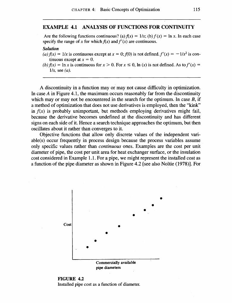
Objective functions that allow only discrete values of the independent variable(~) occur frequently in process design because the process variables assume only specific values rather than continuous ones. Examples are the cost per unit diameter of pipe, the cost per unit area for heat exchanger surface, or the insulation cost considered in Example 1.1. For a pipe, we might represent the installed cost as a function of the pipe diameter as shown in Figure 4.2 [see also Noltie (1978)l. For

pipe diameters

Cost

FIGURE 4.2 Installed pipe cost as a function of diameter.

Commercially available

PART I1 : Optimization Theory and Methods

Diameter

FIGURE 4.3 Piecewise linear approximation to cost function.

most purposes such a cost function can be approximated as a continuous function because of the relatively small differences in available pipe diameters. You can then disregard the discrete nature of the function and optimize the cost as if the diameter were a continuous variable. For example, extend the function of Figure 4.2 to a continuous range of diameters by interpolation. If linear interpolation is used, then the extended function usually has discontinuous derivatives at each of the original diameters, as shown in Figure 4.3. As mentioned earlier, this step can cause problems for derivative-based optirnizers. A remedy is to interpolate with quadratic or cubic functions chosen so that their first derivatives are continuous at the break points. Such functions are called splines (Bartela et al., 1987). Once the optimum value of the diameter is obtained for the continuous function, the discretely valued diameter nearest to the optimum that is commercially available can be selected. A suboptimal value for installed cost results, but such a solution should be adequate for engineering purposes because of the narrow intervals between discrete values of the diameter.

EXAMPLE 4.2 OPTIMIZATION INVOLVING AN INTEGER- VALUED VARIABLE

Consider a catalytic regeneration cycle in which there is a simple trade-off between costs incurred during regeneration and the increased revenues due to the regenerated catalyst. Let x , be the number of days during which the catalyst is used in the reactor and x2 be the number of days for regeneration. The reactor start-up crew is only available in the morning shift, so x, + x, must be an integer.

We assume that the reactor feed flow rate q (kglday) is constant as is the cost of the feed C, ($/kg), the value of the product C2 ($/kg), and the regeneration cost C,


($/regeneration cycle). We further assume that the catalyst deteriorates gradually according to the linear relation

where 1.0 represents the weight fraction conversion of feed at the start of the operat- ing cycle, and k is the deterioration factor in units of weight fraction per day. Define an objective function and find the optimal value of x,.

Solution. For one complete cycle of operation and regeneration, the objective function for the total profit per day comprises

Profit -- - Product value - Feed cost Day

- (Regeneration cost per cycle) (Cycles per day)

or in the defined notation

where dav, = 1.0 - (kx1/2). The maximum daily profit for an entire cycle is obtained by maximizing Equa-

tion (a) with respect to x,. As a first trial, we allow x, to be a continuous variable. When the first derivative of Equation (a) is set equal to zero and the resulting equation solved for x,, the optimum is

Suppose x2 = 2, k , = 0.02, q = 1000, C,= 1.0, C, = 0.4, and C, = 1000. Then xlOp' = 12.97 (rounded to 13 days if x, is an integer).

Clearly, treating x, as a continuous variable may be improper if x, is 1, 2, 3, and so on, but is probably satisfactory if x, is 15, 16, 17, and so on. You might specify x, in terms of shifts of 4-8 h instead of days to obtain finer subdivisions of time.

In real life, other problems involving discrete variables may not be so nicely posed. For example, if cost is a function of the number of discrete pieces of equipment, such as compressors, the optimization procedure cannot ignore the integer character of the cost function because usually only a small number of pieces of equipment are involved. You cannot install 1.54 compressors, and rounding off to 1 or 2 compressors may be quite unsatisfactory. This subject will be discussed in more detail in Chapter 9.

118 PART 11: Optimization Theory and Methods

4.2 NLP PROBLEM STATEMENT

A general form for a nonlinear program (NLP) is

Minimize: f (x) Subject to: a i 5 gi(x) 5 bi i = 1, . . . , m

and lj 5 xi 5 u j j = 1, . . . , n

In this problem statement, x is a vector of n decision variables (x,, . . . , x,), f is the objective function, and the g, are constraint functions. The a, and bi are specified lower and upper bounds on the constraint functions with a, 5 b, and $, uj are lower and upper bounds on the variables with 1, 5 u,. If ai = bi, the ith constraint is an equality constraint. If the upper and lower limits on gi correspond to a, = -00 and b, = +m, the constraint is unbounded. Similar comments apply to the variable bounds, with 1, = uj corresponding to a variable xj whose value is fixed, and 1, = -m and uj = +oo specifying a free variable.

Problem 4.1 is nonlinear if one or more of the functionsf, g,, . . . , g, are nonlinear. It is unconstrained if there are no constraint functions g, and no bounds on the xi, and it is bound-constrained if only the xi are bounded. In linearly constrained problems all constraint functions gi are linear, and the objective f is nonlinear. There are special NLP algorithms and software for unconstrained and bound-constrained problems, and we describe these in Chapters 6 and 8. Methods and software for solving constrained NLPs use many ideas from the unconstrained case. Most mod- ern software can handle nonlinear constraints, and is especially efficient on linearly constrained problems. A linearly constrained problem with a quadratic objective is called a quadratic program (QP). Special methods exist for solving QPs, and these are often faster than general purpose optimization procedures.

A vector x is feasible if it satisfies all the constraints. The set of all feasible points is called the feasible region F. If F is empty, the problem is infeasible, and if feasible points exist at which the objective f is arbitrarily large in a max problem or arbitrarily small in a min problem, the problem is unbounded. A point (vector) x* is termed a local extremum (minimum) if

for all x in a small neighborhood (region) N in F around x* with x distinct from x*. Despite the fact that x* is a local extremum, other extrema may exist outside the neighboorhood N meaning that the NLP problem may have more that one local minimum if the entire space of x is examined. Another important concept relates to the idea of a global extremum, the unique solution of the NLP problem. A global minimum occurs if Equation (4.2) holds for all x E E Analogous concepts exist for local maxima and the global maximum. Most (but not all) algorithms for solving NLP problems locate a local extremum from a given starting point.

NLP geometry A typical feasible region for a problem with two variables and the constraints

c HA PTER 4: Basic Concepts of Optimization

FIGURE 4.4 Feasible region (region not shaded and its boundaries).

is shown as the unshaded region in Figure 4.4. Its boundaries are the straight and curved lines xj = 0 and gi(x) = 0 for i = 1,2, j = 1, 2.

As another example, consider the problem

Minimize f = (xI - 3)2 + (x2 - 4)2

subject to the linear constraints

This problem is shown in Figure 4.5. The feasible region is defined by linear constraints with a finite number of corner points. The objective function, being nonlinear, has contours (the concentric circles, level sets) of constant value that are not parallel lines, as would occur if it were linear. The minimum value off corresponds to the contour of lowest value having at least one point in common with the feasible region, that is, at x,* = 2, x2* = 3. This is not an extreme point of the feasible set, although it is a boundary point. For linear programs the minimum is always at an extreme point, as shown in Chapter 7.

Furthermore, if the objective function of the previous problem is changed to

PART 11: Optimization Theory and Methods

FIGURE 4.5 The minimum occurs on the boundary of the constraint set.

as depicted in Figure 4.6, the minimum is now at x, = 2, x, = 2, which is not a boundary point of the feasible region, but is the unconstrained minimum of the nonlinear function and satisfies all the constraints.

Neither of the problems illustrated in Figures 4.5 and 4.6 had more than one optimum. It is easy, however, to construct nonlinear programs in which local optima occur. For example, if the objective function f, had two minima and at least one was interior to the feasible region, then the constrained problem would have two local minima. Contours of such a function are shown in Figure 4.7. Note that the minimum at the boundary point x, = 3, x2 = 2 is the global minimum at f = 3; the feasible local minimum in the interior of the constraints is at f = 4.

Although the examples thus far have involved linear constraints, the chief nonlinearity of an optimization problem often appears in the constraints. The feasible region then has curved boundaries. A problem with nonlinear constraints may have local optima, even if the objective function has only one unconstrained optimum. Consider a problem with a quadratic objective function and the feasible region shown in Figure 4.8. The problem has local optima at the two points a and b because no point of the feasible region in the immediate vicinity of either point yields a smaller value off.

CHAPTER 4: Basic Concepts of Optimization

FIGURE 4.6 The minimum occurs in the interior of the constraint set.

In summary, the optimum of a nonlinear programming problem is, in general, not at an extreme point of the feasible region and may not even be on the boundary. Also, the problem may have local optima distinct from the global optimum. These properties are direct consequences of nonlinearity. A class of nonlinear problems can be defined, however, that are guaranteed to be free of distinct local optima. They are called convex programming problems and are considered in the following section.

4.3 CONVEXITY AND ITS APPLICATIONS

The concept of convexity is useful both in the theory and applications of optirniza- tion. We first define a convex set, then a convexfunction, and lastly look at the role played by convexity in optimization.

Convex set A set of points (or a region) is defined as a convex set in n-dimensional space

if, for all pairs of points x, and x, in the set, the straight-line segment joining them is also entirely in the set. Figure 4.9 illustrates the concept in two dimensions.


FIGURE 4.7 Local optima due to objective function.

A mathematical statement of a convex set is

For every pair of points x1 and x2 in a convex set, the point x given by a linear combination of the two points

x = yx, + (1 - y)x, 0 5 y 5 1

is also in the set. The convex region may be closed (bounded) by a set of functions, such as the sets A and B in Figure 4.9 or may be open (unbounded) as in Figures 4.10 and 4.12. Also, the intersection of any number of convex set is a convex set.

Convex function Next, let us examine the matter of a convexfunction. The concept of a convex

function is illustrated in Figure 4.10 for a function of one variable. Also shown is a concave function, the negative of a convex function. (If f (x) is convex, - f (x) is concave.) A function f (x) defined on a convex set F is said to be a convexfunction if the following relation holds


FIGURE 4.8 Local optima due to feasible region.

where y is a scaler with the range 0 5 y 5 1. If only the inequality sign holds, the function is said to be not only convex but strictly convex. [If f ( x ) is strictly convex, -f (x ) is strictly concave.] Figure 4.10 illustrates both a strictly convex and a strictly concave function. A convex function cannot have any value larger than the values of the function obtained by linear interpolation between x, and x, (the cord between x, and x, shown in the top figure in Figure 4.10). Linear functions are both convex and concave, but not strictly convex or concave, respectively. An important result of convexity is

If f ( x ) is convex, then the set

is convex for all scalers k.

The result is illustrated in Figure 4.11 in which a convex quadratic function is cut by the plane f (x ) = k. The convex set R projected on to the x,-x, plane comprises the boundary ellipse plus its interior.

The convex programming problem An important result in mathematical programming evolves from the concept of

convexity. For the nonlinear programming problem called the convex programming problem

Minimize: f ( x ) Subject to: gi(x) 5 0 i = 1, . . . , m


Convex set

Convex set

Nonconvex set All of the line a segment is ,not in the set

FIGURE 4.9 Convex and nonconvex sets.

in which (a) f(x) is a convex function, and (b) each inequality constraint is a convex function (so that the constraints form a convex set), the following property can be shown to be true

The local minimum off (x) is also the global minimum.

Analogously, a local maximum is the global maximum off (x) if the objective function is concave and the constraints form a convex set.

Role of convexity If the constraint set g(x) is nonlinear, the set

R = {xlg(x) = 0)

is generally not convex. This is evident geometrically because most nonlinear functions have graphs that are cumed surfaces. Hence the set R is usually a curved surface also, and the line segment joining any two points on this surface generally does not lie on the surface.


X1 x2 Convex function

Concave function

Convex function

FIGURE 4.10 Convex and concave functions of one variable.


Convex function Convex function

Plane f (x) = k

I I I I I I I I I I

FIGURE 4.11 Illustration of a convex set formed by a plane f(x) = k cutting a convex function.

As a consequence, the problem

Minimize: f (x) g i (x ) 5 0 i = 1, ...,. m

Subject to: h,(x) = 0 k = 1, ..., r < n

may not be a convex programming problem in the variables x,, . . . , x, if any of the functions hk(x) are nonlinear. This, of course, does not preclude efficient solution of such problems, but it does make it more diff~cult to guarantee the absence of local optima and to generate sharp theoretical results.

In many cases the equality constraints may be used to eliminate some of the variables, leaving a problem with only inequality constraints and fewer variables. Even if the equalities are difficult to solve analytically, it may still be worthwhile solving them numerically. This is the approach taken by the generalized reduced gradient method, which is described in Section 8.7.

Although convexity is desirable, many real-world problems turn out to be nonconvex. In addition, there is no simple way to demonstrate that a nonlinear problem is a convex problem for all feasible points. Why, then is convex programming stud- ied? The main reasons are

1. When convexity is assumed, many significant mathematical results have been derived in the field of mathematical programming.

2. Often results obtained under assumptions of convexity can give insight into the properties of more general problems. Sometimes, such results may even be car- ried over to nonconvex problems, but in a weaker form.

c H APTER 4: Basic Concepts of Optimization 127

For example, it is usually impossible to prove that a given algorithm will find the global minimum of a nonlinear programming problem unless the problem is convex. For nonconvex problems, however, many such algorithms find at least a local minimum. Convexity thus plays a role much like that of linearity in the study of dynamic systems. For example, many results derived from linear theory are used in the design of nonlinear control systems.

Determination of convexity and concavity The definitions of convexity and a convex function are not directly useful in

establishing whether a region or a function is convex because the relations must be applied to an unbounded set of points. The following is a helpful property arising from the concept of a convex set of points. A set of points x satisfying the relation

is convex if the Hessian matrix H(x) is a real symmetric positive-semidefinite matrix. H(x) is another symbol for V2f(x), the matrix of second partial derivative of f(x) with respect to each xi

H(x) = H = vf (x)

The status of H can be used to identify the character of extrema. A quadratic form Q(x) = X ~ H X is said to be positive-definite if Q(x) > 0 for all x # 0, and said to be positive-semidefinite if Q(x) 2 0 for all x # 0. Negative-definite and negative- semidefinite are analogous except the inequality sign is reversed. If Q(x) is positive- definite (semidefinite), H(x) is said to be a positive-definite (semidefinite) matrix. These concepts can be summarized as follows:

1. H is positive-definite if and only if xTHx is > 0 for all x # 0 . 2. H is negative-definite if and only if x T ~ x is < 0 for all x # 0 . 3. H is positive-semidefinite if and only if x T ~ x is 2 0 for all x # 0 . 4. H is negative-semidefinite if and only if xTHx is 0 for all x # 0 . 5. H is indefinite if X ~ H X < 0 for some x and > 0 for other x.

It can be shown from a Taylor series expansion that if f(x) has continuous second partial derivatives, f(x) is concave if and only if its Hessian matrix is negative- semidefinite. For f (x) to be strictly concave, H must be negative-definite. For f(x) to be convex H(x) must be positive-semidefinite and for f (x) to be strictly convex, H(x) must be positive-definite.

EXAMPLE 4.3 ANALYSIS FOR CONVEXITY AND CONCAVITY

For each of these functions (a) f ( x ) = 3x2 (b) f ( x ) = 2x -. (c) f ( x ) = -5x2 (d) f ( x ) = 2x2 - x 3

128 PART I1 : Optimization Theory and Methods

determine if f(x) is convex, concave, strictly convex, strictly concave, all, or none of these classes in the range - m 5 x 5 m.

Solution (a) f "(x) = 6, always positive, hence f(x) is both strictly convex and convex. (b) f "(x) = 0 for all values of x, hence f(x) is convex and concave. Note straight

lines are both convex and concave simultaneously. (c) f "(x) = - 10, always negative, hence f(x) is both strictly concave and concave. (d) f "(x) = 6 - 3x; may be positive or negative depending on the value of x, hence

f(x) is not convex or concave over the entire range of x.

For a multivariate function, the nature of convexity can best be evaluated by examining the eigenvalues of f(x) as shown in Table 4.1 We have omitted the indefinite case for H, that is when f(x) is neither convex or concave.

TABLE 4.1 Relationship between the character of f(x) and the

state of H(x)

All the eigenvalues of H(x) are

Strictly convex Positive-definite >O Convex Positive-semidefinite 20

Concave Negative-semidefinite 10 Strictly concave Negative-definite <O

Now let us further illustrate the ideas presented in this section by some examples.

EXAMPLE 4.4 DETERMINATION OF POSITIVE-DEFINITENESS OF A FUNCTION

Classify the function f(x) = 2xT - 3xlx2 + 2 4 using the categories in Table 4.1, or state that it does not belong in any of the categories.

Solution

af ( 4 -- ' - h i - 3x2

, a'f(x> -- a?f(x> - 4 -- - 4 8x1 ax: ax;

The eigenvalues of H are 7 and 1, hence H(x) is positive-definite. Consequently,JTx) is strictly convex (as well as convex).


EXAMPLE 4.5 DETERMINATION OF POSITIVE-DEFINITENESS OF A FUNCTION

Repeat the analysis of Example 4.4 forflx) = x12 + x,x2 + 2x2 + 4

Sobtion

The eigenvalues are 1 + fi and 1 - fi , or one positive or one negative value. Consequently, fix) does not fall into any of the categories in Table 4.1. We conclude that no unique extremum exists.

EXAMPLE 4.6 DETERMINATION OF CONVEXITY AND CONCAVITY

Determine if the following function

flx) = 2x1 + 3x2 + 6 is convex or concave.

Solution

hence the function is both convex and concave.

EXAMPLE 4.7 DETERMINATION OF CONVEXITY OF A FUNCTION

Consider the following objective function: Is it convex?

AX) = 2x; + 2x1x2 + 1.5~; + 7x1 + 8x2 + 24 Solution

a X x > -- ax~> - 3 ---- a2f(x> - - - ----- a'f(x> - - 4 ---- - 2 ax: ax; axiax2 ax2ax1

Therefore the Hessian matrix is

The eigenvalues of H(x) are 5.56 and 1.44. Because both eigenvalues are positive, the function is strictly convex (and convex, of course) for all values of x1 and x2.

130 PART 11 : Optimization Theory and Methods

EXAMPLE 4.8 DETECTION OF A CONVEX REGION

Does the following set of constraints that form a closed region form a convex region? 2 - x l + x2 I 1

x , - x2 1 - 2

Solution. A plot of the two functions indicates that the region circumscribed is closed. The arrows in Figure E4.8 designate the directions in which the inequalities hold. Write the inequality constraints as gi 2 0. Therefore

g , (x ) = X l - X2 + 2 L 0

That the enclosed region is convex can be demonstrated by showing that both g l (x ) and g2(x) are concave functions:

negative definite

negative semidefinite

Because all eigenvalues are zero or negative, according to Table 4.1 both g, and g2 are concave and the region is convex.

FIGURE E4.8 Convex region composed of two concave functions.


EXAMPLE 4.9 CONSTRUCTION OF A CONVEX REGION

Construct the region given by the following inequality constraints; is it convex?

x, 1 6; x2 5 6; x1 r 0; xl + x2 I 6; x2 2 0

Solution. See Figure E4.9 for the region delineated by the inequality constraints. By visual inspection, the region is convex. This set of linear inequality constraints forms a convex region because all the constraints are concave. In this case the convex region is closed.

FIGURE E4.9 Diagram of region defined by linear inequality constraints.

4.4 INTERPRETATION OF THE OBJECTIVE FUNCTION IN TERMS OF ITS QUADRATIC APPROXIMATION

If a function of two variables is quadratic or approximated by a quadratic function f(x) = b, + blxl + bg2 + bllx: + b22xg + b,2xlx2, then the eigenvalues of H(x) can be calculated and used to interpret the nature offlx) at x*. Table 4.2 lists some conclusions that can be reached by examining the eigenvalues of H(x) for a function of two variables, and Figures 4.12 through 4.15 illustrate the different types of surfaces corresponding to each case that arises for quadratic function. By


TABLE 4.2

Geometric interpretation of a quadratic function

Character of Eigenvalue Signs Qpes of Geometric center of

Case relations el e, contours interpretation contours Figure

Circles Circular hill Circles Circular valley Ellipses Elliptical hill Ellipses Elliptical valley Hyperbolas Symmetrical

saddle Hyperbolas Symmetrical

saddle Hyperbolas Elongated saddle Straight lines Stationary ridge* Straight lines Stationary valley* Parabolas Rising ridge** Parabolas Falling valley*$

Maximum Minimum Maximum Minimum Saddle point

Saddle point

Saddle point None None Atm At 00

*These are "degenerate" surfaces. *The condition of rising or falling must be evaluated from the linear terms in f(x).

FIGURE 4.12 Geometry of a quadratic objective function of two independent variables-elliptical contours. If the eigenvalues are equal, then the contours are circles.

implication, analysis of a function of many variables via examination of the eigenvalues can be conducted, whereas contour plots are limited to functions of only two or three variables.


FIGURE 4.13 Geometry of a quadratic objective function of two independent variables-saddle point.

FIGURE 4.14 Geometry of a quadratic objective function of two independent variables-stationary valley.


FIGURE 4.15 Geometry of second-order objective function of two independent variables- falling valley.

Figure 4.12 corresponds to objective functions in well-posed optimization problems. In Table 4.2, cases 1 and 2 correspond to contours off (x) that are concentric circles, but such functions rarely occur in practice. Elliptical contours such as correspond to cases 3 and 4 are most likely for well-behaved functions. Cases 5 to 10 correspond to degenerate problems, those in which no finite maximum or minimum or perhaps nonunique optima appear.

For well-posed quadratic objective functions the contours always form a convex region; for more general nonlinear functions, they do not (see Qe next section for an example). It is helpful to construct contour plots to assist in analyzing the performance of multivariable optimization techniques when applied to problems of two or three dimensions. Most computer libraries have contour plotting routines to generate the desired figures.

As indicated in Table 4.2, the eigenvalues of the Hessian matrix ofJTx) indicate the shape of a function. For a positive-definite symmetric matrix, the eigenvectors (refer to Appendix A) form an orthonormal set. For example, in two dimensions, if the eigenvectors are v, and v,, v:v2 = 0 (the eigenvectors are perpendicular to each other). The eigenvectors also correspond to the directions of the principal axes of the contours of JTx).

One of the primary requirements of any successful optimization technique is the ability to move rapidly in a local region along a narrow valley (in minimiza- tion) toward the minimum of the objective function. In other words, an efficient algorithm selects a search direction that generally follows the axis of the valley rather than jumping back and forth across the valley. Valleys (ridges in maximiza- tion) occur quite frequently, at least locally, and these types of surfaces have the potential to slow down greatly the search for the optimum. A valley lies in the direction of the eigenvector associated with a small eigenvalue of the Hessian

\


matrix of the objective function. For example, if the Hessian matrix of a quadratic function is

then the eigenvalues are el = 1 and e, = 10. The eigenvector associated with el = 1, that is, the x, axis, is lined up with the valley in the ellipsoid. Variable transfor- mation techniques can be used to allow the problem to be more efficiently solved by a search technique (see Chapter 6).

Valleys and ridges corresponding to cases 1 through 4 can lead to a minimum or maximum, respectively, but not for cases 8 through 11. Do you see why?

4.5 NECESSARY AND SUFFICIENT CONDITIONS FOR AN EXTREMUM OF AN UNCONSTRAINED FUNCTION

Figure 4.16 illustrates the character offlx) if the objective function is a function of a single variable. Usually we are concerned with finding the minimum or maximum of a multivariable functionflx). The problem can be interpreted geometrically as b d - . ing the point in an n-dimension space at which the function has an extremum. Exarn- ine Figure 4.17 in which the contours of a function of two variables are displayed.

An optimal point x* is completely specified by satisfying what are called the necessary and suficient conditions for optimality. A condition N is necessary for a result R if R can be true only if .the condition is true (R + N). The reverse is not true, however, that is, if N is true, R is not necessarily true. A condition is sufficient for a result R if R is true if the condition is true (S =s R ) . A condition T is necessary and sufficient for result R if R is true if and only if T is true (T * R ) .

X

FIGURE 4.16 A function exhibiting different types of stationary points. Key: a-inflection point (scalar equivalent to a saddle point); b-global maximum (and local maximum); c-local minimum; d-local maximum


FIGURE 4.17a A function of two variables with a single stationary point (the extremum).

The easiest way to develop the necessary and sufficient conditions for a minimum or maximum offlx) is to start with a ~ a ~ l o i series expansion about the pre- sumed extremum x*

where Ax = x - x*, the perturbation of x from x*. We assume all terms in Equa- tion (4.4) exist and are continuous, but will ignore the terms of order 3 or higher [03(Ax)], and simply analyze what occurs for various cases involving just the terms through the second order.

We defined a local minimum as a point x* such that no other point in the vicinity of x* yields a value offlx) less than f (x*), or

Ax) - Ax*) 2 0 (4.5)

x* is a global minimum if Equation (4.5) holds for any x in the n-dimensional space of x. Similarly, x* is a local maximum if


FIGURE 4.17b A function of two variables with three stationary points and two extrema, A and B.

Examine the second term on the right-hand side of Equation (4-4): VTf(x*) Ax. Because Ax is arbitrary and can have both plus and minus values for its elements, we must insist that Vf (x*) = 0. Otherwise the resulting term added to f(x*) would violate Equation (4.5) for a minimum, or Equation (4.6) for a maximum. Hence, a necessary condition for a minimum or maximum off (x) is that the gradient off (x) vanishes at x*

that is, x* is a stationary point. With the second term on the right-hand side of Equation (4.4) forced to be zero,

we next examine the third term: AX^) vf (x*) Ax. This term establishes the character of the stationary point (minimum, maximum, or saddle point). In Figure 4.17b, A and B are minima and C is a saddle point. Note how movement along one of the perpendicular search directions (dashed lines) from point C increasesflx), whereas movement in the other direction decreases f (x). Thus, satisfaction of the necessary conditions does not guarantee a minimum or maximum.

To establish the existence of a minimum or maximum at x*, we know from Equation (4.4) with Vf (x*) = 0 and the conclusions reached in Section 4.3 con- cerning convexity that for Ax # 0 we have the following outcomes


Vzf(x*) = H(x*) AxT V2f(x*) AX Near x*, f(x) - f(x*)

Positive-define >O Increases Positive-semidefinite 20 Possibly increases Negative-definite <O Decreases Negative-semidefinite 5 0 Possibly decreases Indefinite Both 10 and 8 0 Increases, decreases, neither

depending on Ax

Consequently, x* can be classified as

Positive-definite Unique ("isolated") minimum Negative-definite Unique ("isolated") maximum

These two conditions a& known as the suficiency conditions. In summary, the necessary conditions (items 1 and 2 in the following list) and

the sufficient condition (3) to guarantee that x* is an extremum are as follows:

1. flx) is twice differentiable at x*. 2. Vf(x*) = 0, that is, a stationary point exists at x*. 3. H(x*) is positive-definite for a minimum to exist at x*, and negative-definite for

a maximum to exist at x*.

Of course, a minimum or maximum may exist at x* even though it is not possible to demonstrate the fact using the three conditions. For example, iffix) = f13, x* = 0 is a minimum but H(0) is not defined at x* = 0, hence condition 3 is not satisfied.

EXAMPLE 4.10 CALCULATION OF A MINIMUM OF f (x)

Does f(x) = x! have an extremum? If so, what is the value of x* and f(x*) at the extremum?

Solution

fl(x) =4x3 f"(x) = 1 2 2

Set f '(x) = 0 and solve for x; hence x = 0 is a stationary point. Also, fl'(0) = 0, meaning that condition 3 is not satisfied. Figure E4.10 is a plot ofJTx) = 2. Thus, a rnini- mum exists for f (x) but the sufficiency condition is not satisfied.

If both first and second derivatives vanish at the stationary point, then further analysis is required to evaluatk the nature of the function. For functions of a single variable, take successively higher derivatives and evaluate them at the stationary point. Continue this procedure until one of the higher derivatives is not zero (the nth one); hence, f '(x*), f"(x*), . . . , f("-')(x*) all vanish. Two cases must be analyzed:

1. If n is even, the function attains a maximum or a minimum; a positive sign of fen) indicates a minimum, a negative sign a maximum.

2. If n is odd, the function exhibits a saddle point.

For more details refer to Beveridge and Schechter (1970).


FIGURE E4.10

For application of these guidelines toflx) = 2, you will find &JTx)ld$ = 24 for which n is even and the derivative is positive, so that a minimum exists.

EXAMPLE 4.11 CALCULATION OF EXTREMA

Identify the stationary points of the following function (Fox, 1971), and determine if any extrema exist.

Solution. For this function, three stationary points can be located by setting V'x) = 0:

The set of nonlinear equations (a) and (b) has to be solved, say by Newton's method, to get the pairs (x,, x,) as follows:

Stationary point Hessian matrix Point (XI, xz> f ( 4 eigenvalues Classification

B (1.941, 3.854) 0.9855 37.03 0.97 Localminimum

A (- 1.053, 1.028) -0.5134 10.5. 3.5 Local minimum (also the global minimum)

C (0.61 17, 1.4929) 2.83 7.0 -2.56 Saddle point

Figure 4.17b shows contours for the objective function in this example. Note that the global minimum can only be identified by evaluating f (x) for all the local minima.


For general nonlinear objective functions, it is usually difficult to ascertain the nature of the stationary points without detailed examination of each point. '

EXAMPLE 4.12

In many types of processes such as batch constant-pressure filtration or fixed-bed ion exchange, the production rate decreases as a function of time. At some optimal time topt, production is terminated (at POPt) and the equipment is cleaned. Figure E4.12a illustrates the cumulative throughput P(t) as a function of time t for such a process. For one cycle of production and cleaning, the overall production rate is

where R(t) = the overall productioq rate per cycle (massltime) t, = the cleaning time (assumed to be constant)

- . Determine the maximum production rate and show that POPt is indeed the maxi-

mum throughout.

Solution. Differentiate R(t) with respect to t, and equate the derivative to 0:

dR(t) - P(t) + [dP(t)/dt](t + t,) -- - = 0 dt (t + t J 2

The geometric interpretation of Equation (b) is the classical result (Walker et al., 1937) that the tangent to P(t) at P e t intersects the time axis at - t,. Examine Figure E4.12b. The maximum overall production rate is

FIGURE E4.12a

c HA PTER 4: Basic Concepts of Optimization 141

FIGURE E4.12b

FIGURE E4.12~

negative

Does POPt meet the sufficiency condition to be a maximum? Is

d 2 ~ ( t ) - 2P(t) - 2[dP(t)/dt](t + t,) + [d2p(t)/dt2](t + tc)2 - < o ? (d)

dt2 ( t + tCl3

Rearrangement of (4 and introduction of (b) into (d), or the pair (P"pt, tOpt), gives


From Figure E4.12b we note in the range 0 < t< t"pt that dP(t)ldt is always positive and decreasing so that d2P(t)ldt2 is always negative (see Figure E4.12~). Conse- quently, the sufficiency condition is met.

REFERENCES

Bartela, R.; J. Beatty; and B. Barsky. An Introduction to Splines for Use in Computer Graph- ics and Geometric Modeling. Morgan Kaufman Publishers, Los Altos, CA (1987).

Beveridge, G. S. G.; and R. S. Schechter. Optimization: Theory and Practice, McGraw-Hill, New York (1970), p. 126.

Fox, R. L. Optimization Methods for Engineering Design. Addison-Wesley, Reading, MA (1971), p. 42.

Happell, J.; and D. G. Jordan. Chemical Process Economics. Marcel Dekker, New York (1975), p. 178.

Kaplan, W. Maxima and Minima with Applications: Practical Optimization and Duality. Wiley, New York (1 998).

Nash, S. G.; and A. Sofer. Linear and Nonlinear Programming. McGraw-Hill, New York (1996).

Noltie, C. B. Optimum Pipe Size Selection. Gulf Publ. Co., Houston, Texas (1978). Walker, W. H.; W. K. Lewis; W. H. McAdams; and E. R. Gilliland. Principles of Chemical

Engineering. 3d ed. McGraw-Hill, New York (1937), p. 357.

SUPPLEMENTARY REFERENCES

Amundson, N. R. Mathematical Methods in Chemical Engineering: Matrices and Their Application. Prentice-Hall, Englewood Cliffs, New jersey (1966).

Avriel, M. Nonlinear Programming. Prentice-Hall, Englewood Cgffs, New Jersey (1976). Bazarra, M. S.; H. D. Sherali; and C. M. Shetty. Nonlinear Programming: Theory andAlgo-

rithms. Wiley, New York (1993). Borwein, J.; and A. S. Lewis. Convex Analysis and Nonlinear Optimization. Springer, New

York (1999). Jeter, M. W. Mathematical Programming. Marcel Dekker, New York (1986). Luenberger, D. G. Linear and Nonlinear Programming. 2nd ed. Addison-Wesley, Menlo

Park, CA (1984).

PROBLEMS

4.1 Classify the following functions as continuous (specify the range) or discrete: (a) f ( 4 = ex (b) f (x) = ax,-, + b(xo - x,) where x, represents a stage in a distillation column

XD - xs (c) f ( x ) = where x, = concentration of vapor from a still and x, is the

+ xs concentration in the still


4.2 The future worth S of a series of n uniform payments each of amount P is

where i is the interest rate per period. If i is considered to be the only variable, is it discrete or continuous? Explain. Repeat for n. Repeat for both n and i being variables.

4.3 In a plant the gross profit P in dollars is

where n = the number of units produced per year S = the sales price in dollars per unit V = the variable cost of production in dollars per unit F = the fixed charge in dollars

Suppose that the average unit cost is calculated as

n V + F Average unit cost =

n

Discuss under what circumstances n can be treated as a continuous variable.

4.4 One rate of return is the ratio of net profit P to total investment

where t = the fraction tax rate I = the total investment in dollars

Find the maximum R as a function of n for a given I if n is a continuous variable. Repeat if n is discrete. (See Problem 4.3 for other notation.)

4.5 Rewrite the following linear programming problems in matrix notation.

(a) Minimize: f ( x ) = 3x1 + 2 . ~ 2 + x3

Subject to: g , ( x ) = 2x1 3x2 + x3 2 10

g2(x) = X I + 2x2 + ~3 2 15

(b) Maximize: f ( x ) = 5x1 + 10x2 + 1 h 3

Subject to: g , (x ) = 15xl + lox2 + lox3 5 200

g,(x) = X , 2 o g3(x) = x2 2 0

4.6 Put the following nonlinear objective function into matrix notation by defining suitable matrices; x = [x, x21T.

f ( x ) = 3 + 2x1 + 3x2 + 2x: + 2 ~ ~ x 2 + 6x;


4.7 Sketch the objective function and constraints of the following nonlinear programming problems.

(a) Minimize: f(x) = 2xf - 2~1x2 + 2 ~ ; - 6x1 + 6

Subject to: gl(x) = x1 + x2 5 2

(b) Minimize: f(x) = x: - 3x1x2 + 4

Subject to: gl(x) = 5x1 + 2x2 2 18

h,(x) = - 2x1 + x; = 5

(c) Minimize: f(x) = -5x: + x;

x; 1 Subjectto: gl(x) = 7 - - 5 -1

x2 x2

g2(x) = xl 2 0

g3(x) = X2 2 0

4.8 Distinguish between the local and global extrema of the following objective function.

f(x) = 2x: + x; + x:x; + 4x1x2 + 3

4.9 Are the following vectors (a) feasible or nonfeasible vectors with regard to Problem 4.5b; (b) interior or exterior vectors?

(1) x = [5 2 10IT

(2) x = [lo 2 7.5IT

(3) x = [0 0 OIT

4.10 Shade the feasible region of the nonlinear programming problems of Problem 4.7. Is x = [I 1lT an interior, boundary, or exterior point in these problems?

4.11 What is the feasible region for x given the following constraints? Sketch the feasible region for the two-dimensional problems.

(a) hl(x) = x1 + x2 - 3 = 0

h2(x) = 2x1 - x2 + 1 = 0

(b) hl(x) = x: + x i + x; = 0

h2(x) = x1 + x2 + x3 = 0

(c) gl(x) = XI - x; - 2 2 0

g2(x) = X1 - X2 + 4 2 0

(d) h,(x) = x:+xg + 3

gl(x) = XI - X2 + 2 2 0

g2(x) = X1 2 0

g3(x) = X2 2 0


4.12 Two solutions to the nonlinear programming problem

Minimize: f (x) = 7x1 - 6x2 + 4x3

Subject to: hl(x) = x: + 2.x; + 3x; - 1 = 0

h2(x) = 5x1 + 5x2 - 3x3 - 6 = 0

have been reported, apparently a maximum and a minimum.

Verify that each of these x vectors is feasible.

4.13 The problem Minimize: f(x) = 100(x,-~:)~ + (1 -xl) ,

Subject to: x: + x; 5 2 is reported to have a local minimum at the point x* = [l 1IT. Is this local optimum also a global optimum?

4.14 Under what circumstances is a local minimum guaranteed to be the global minimum? (Be brief.)

4.15 Are the following functions convex? Strictly convex? Why?

(a) 2x: + 2xlx2 + 3x; + 7x1 + 8x2 + 25

What are the optimum values of x1 and x,?

(b) e5"

4.16 Determine the convexity or concavity of the following objective functions:

(a) f(x19xz) = (XI + X:

(b) f(x,,x,, x3) = x: + x; + x:

(c) f ( ~ 1 , ~ 2 ) = 62 X I + ex2

4.17 Show that f = exl + ex2 is convex. Is it also strictly convex?

4.18 Show that f = 1x1 is convex.

4.19 Is the following region constructed by the four constraints convex? Closed?


4.20 Does the following set of constraints form a convex region?

4.21 Consider the following problem:

Minimize: f ( x ) = x f + x2

Subject to: g l ( x ) = x: + x: - 9 5 0

g2(x) = ( x , + x i ) - 1 5 0

: Does the constraint set form a convex region? Is it closed? (Hint: A plot will help you decide.)

4.22 Is the following function convex, concave, neither, or both? Show your calculations.

f ( x ) = In xl + In x2

4.23 Sketch the region defined by the following inequality constraints. Is it a convex region? Is it closed?

X l + X 2 - - 1 1 0

x , - X , + I 2 0

2 - X I 2 0

X 2 2 0

4.24 Does the following constraint set form a convex region (set)?

h ( x ) = x: + x ; - 9 = 0

4.25 Separable functions are those that can be expressed in the form

For example, xp + x i + x: is a separable function because

Show that if the terms in a separable function are convex, the separable function is convex.


4.26 Is the following problem a convex programming problem?

Minimize: 200

f (x) = loox, + - X l X 2

300 ' Subject to: 2x2 + - 5 I

x1x2

4.27 Classify each of the following matrices as (a) positive-definite, (b) negative-definite, (c) neither.

4.28 Determine whether the following matrix is positive-definite, positive-semidefinite, negative-definite, negative-semidefinite, or none of the above. Show all calculations.

4.29 In designing a can to hold a specified amount of soda water, the cost function (to be minimized) for manufacturing one can is

and the constraints are

Based on the preceding problem, answer the following; as far as possible for each answer use mathematics to support your statements: (a) State whether f(D, h) is unimodal (one extremum) or multimodal (more then one

extremum). (b) State whether f(D, h) is continuous or not. (c) State whether f(D, h) is convex, concave, or neither. (d) State whether or not f(D, h) alone meets the necessary and sufficient conditions

for a minimum to exist. (e) State whether the constraints form a convex region.

4.30 A reactor converts an organic compound to product P by heating the material in the presence of an additive A (mole fraction = x,). The additive can be injected into the reactor, while steam can be injected into a heating coil inside the reactor to provide heat. Some conversion can be obtained by heating without addition of A, and vice versa.


The product P can be sold for $50/lb mol. For 1 lb mol of feed, the cost of the additive (in dollars~b mol) as a function of xA is given by the formula, 2.0 + loxA + 20xA2. The cost of the steam (in dollars) as a function of S is 1.0 + 0.003s + 2.0 X S2. (S = lb stearn/lb mol feed). The yield equation is y, = 0.1 + 0 . 3 ~ ~ + 0.001s 4- 0 . 0 0 0 1 ~ ~ S; YP = lb mol product Pllb mol feed.

(a) Formulate the profit function (basis of 1.0 lb mol feed) in terms of xA and S.

f = Income - Costs

The constraints are:

(b) Is f a concave function? Demonstrate mathematically why it is or why it is not concave. (c) Is the region of search convex? Why?

4.31 The objective function for the work requirement for a three-stage compressor can be expressed as (p is pressure)

p, 1 atm and p4 = 10 atrn. The minimum occurs at a pressure ratio for each stage of 6. Is fconvexfor 1 S p , 5 10,l 5 p 3 5 lo?

4.32 In the following problem (a) Is the objective function convex? (b) Is the constraint region convex?

Minimize:

300 g(x) = 2x2 + r i

Subject to: X I + X 2

4.33 Answer the questions below for the following problem; in each case justify your answer.

Minimize: 1 4 1 2 f(x) = 2x1 - 5x1 - X*

Subject to: x: + x i = 4

(a) Is the problem a convex programming problem? (b) Is the point x = [l 1IT a feasible point? (c) Is the point x = [2 2IT an interior point?

4.34 Happel and Jordan (1975) reported an objective function (cost) for the design of a distillation column as follows:

c HA PTER 4: Basic Concepts of Optimization

where n = number of theoretical stages R = reflux ratio P = percent recovery in bottoms stream

They reported the optimum occurs at R = 8, n = 55, and P = 99. Is f convex at this point? Are there nearby regions where f is not convex?

4.35 Given a linear objective function,

f = xl + X2

(x, and x, must lie in region A )

FIGURE P4.35

explain why a nonconvex region such as region A in Figure P4.35 causes difficulties in the search for the maximum off in the region. Why is region A not convex?

4.36 Consider the following objective furiction

Show that f is convex. Hint: Expand f for both n odd and n even. You can plot the function to assist in your analysis. Under what circumstances is

convex?

4.37 Classify the stationary points of

(a) f = - x 4 + x 3 + 20 (b) f = x 3 + 3x2 + x + 5 (c) f = x 4 - 2 x 2 + 1

(d) f = X: - 8x1x2 + X;

according to Table 4.2


4.38 List stationary points and their classification (maximum, minimum, saddle point) of

(a) f = xf + 2x1 + 3x; + 6x2 + 4

(b) f = X l + X2 + X : - 4 ~ ~ x 2 + 2 4

4.39 State what type of surface is represented by

at the stationary point x = [0 OIT (use Table 4.2).

4.40 Interpret the geometry of the following function at its stationary point in terms of Table 4.2

4.41 Classify the following function in terms of the list in Table 4.2:

4.42 In crystal NaCl, each Na+ or C1- ion is surrounded by 6 nearest neighbors of opposite charge and 12 nearest neighbors of the same charge. Two sets of forces oppose each other: the coulombic attraction and the hard-core repulsion. The potential energy u(r) of the crystal is given by the Lennard-Jones potential expression,

where €,a are constants, such that E > 0, a > 0. (a) Does the Lennard-Jones potential u(r) have a stationary point(s)? If it does, lo~ate

it (them). (b) Identify the nature of the stationary point(s) min, max, etc. (c) What is the magnitude of the potential energy at the stationary points?

4.43 Consider the function

Note that x = a minimizes y. Let. z = x2 - 4x + 16. Does the solution to x2 - 4x + 16 = 0,

minimize I? ( j = fi) .

4.44 The following objective function can be seen by inspection to have a minimum at x = 0:

f ( x ) = 1x31


Can the criteria of Section 4.5 be applied to test this outcome?

4.45 (a) Consider the objective function,

Find the stationary points and classify them using the Hessian matrix. (b) Repeat for

(c) Repeat for

4.46 An objective function is

By inspection, you can find x* = [8 5IT yields the minimum of Ax). Show that x* meets the necessary and sufficient conditions for a minimum.

4.47 Analyze the function

Find all of its stationary points and determine if they are maxima, minima, or inflection (saddle) points. Sketch the curve in the region of

4.48 Determine if the following objective function

f(x) = 2: + x ; + x:x; + 4x ,x2 + 3

has local minima or maxima. Classify each point clearly.

4.49 Is the following function unimodal (only one extremum) or multimodal (more than one extremum)?

4.50 Determine whether the solution x = [-0.87 -0.8IT for the objective function

f(x) = x: + 1 2 ; - 1%: - 56x2 + 60

is indeed a maximum.

basic concepts of optimization - university of oklahoma of chemical... · 114 part i i :...

Documents