basic data wrangling in r - github pages
TRANSCRIPT
Chapter 3
Basic Data Wrangling in R
Whether we call it data wrangling, data management, data munging, or even data manip-ulation, the ability to transform data into a format suitable for analysis is an incrediblyvaluable skill. But as data has increased in size, the skills associated with this process havechanged. In the 1990s, pioneers in what we now call data science were making meaningfulcontributions to a wide range of fields using spreadsheets. Today, data scientists write codeto do most of their data wrangling. What has brought about this transition?
Consider the evolution of baseball analytics (often called sabermetrics), which in manyways mirrors the evoluation of analytics in other domains. The use of statistics in baseballhas a long and storied history – in part because the game itself is naturally discrete, andin part because Henry Chadwick began publishing boxscores in the early 1900s [107]. Forthese reasons, a rich catalog of baseball data began to accumulate. However, while moreand more baseball data was piling up, analysis of that data was not so prevalent. That is,the extant data provided a means to keep records, and as a result some numerical elementsof the game’s history took on a life of their own (e.g. Babe Ruth’s 714 home runs). Butit’s not as clear how much people were learning about the game of baseball from the data.Knowing that Babe Ruth hit more home runs than Mel Ott tells us something about twoplayers, but doesn’t provide any insight into the nature of the game itself.
In 1947 – Jackie Robinson’s rookie season – Brooklyn Dodgers’ GM Branch Rickey madeanother significant innovation: he hired Allan Roth to be baseball’s first statistical analyst.Roth’s analysis of baseball data led to insights that the Dodgers used to win more games.In particular, Roth convinced Rickey that a measurement of how often a batter reaches firstbase via any means (e.g. hit, walk, or being hit by the pitch) was a better indicator of thatbatter’s value than how often he reaches first base via a hit (which was – and probably stillis – the most commonly-cited batting statistic). The logic supporting this insight was basedon both Roth’s understanding of the game of baseball (what we call domain knowledge)and his statistical analysis of baseball data.
During the next 50 years, many important contributions to baseball analytics were madeby a variety of people (most notably “The Godfather of Sabermetrics” Bill James [57]), mostof whom had little formal training in statistics, and for most of whom, the weapon of choicewas a spreadsheet. They were able to use their creativity, domain knowledge, and a keensense of what the interesting questions were, in order to make interesting discoveries.
But the 2002 publication of Moneyball [73] – which showcased how Billy Beane andPaul DePodesta used statistical analysis to run the Oakland A’s – triggered a revolutionin how front offices in baseball were managed [11]. Over the next decade, the size of thedata expanded so rapidly that a spreadsheet was no longer a viable mechanism for storing– let alone analyzing – all of the available data. Today, more than a handful of teams have
11
12 CHAPTER 3. BASIC DATA WRANGLING IN R
research and development groups headed by people with Ph.D.’s in statistics or computerscience along with graduate training in machine learning [10].
Thus, the contributions made by the next generation of baseball analysts will requirecoding ability. While the creativity and domain knowledge that fueled the work of AllanRoth and Bill James will remain necessary traits, they are no longer sufficient. And yetthere is nothing special about baseball in this respect. For data scientists of all applicationdomains, creativity, domain knowledge, and technical ability are absolutely essential.
A similar profusion of data is now available in many other areas, including astronomy,health services research, genomics, and climate change, among others.
Previously, we described the five main steps of data science: loading (or ingesting it),manipulation, visualization, modeling, and reporting. In this chapter, we introduce thebasics of how to manage (or wrangle) data in R. These skills will provide a intellectual andpractical foundation for working with modern data.
3.1 The Five Idioms of Single Table Analysis
In his ongoing work to improve’s R flexibility and power for data wrangling [129, 131],Hadley Wickham has identified five idioms for working with data in a single data frame:
1. select : take a subset of the columns (i.e. features, variables)
2. filter : take a subset of the rows (i.e. observations)
3. mutate: add or change columns
4. arrange: sort the rows
5. summarise: aggregate the data across rows (e.g. group it according to some criteria)
These five idioms, used in conjunction with each other, provide a powerful means to slice-and-dice a single table of data. Mastery of these five idioms can make the computation ofmost any descriptive statistic a breeze and facilitate further analysis. Wickham’s approachis inspired by his desire to blur the boundaries between R and the ubiquitous relationaldatabase querying syntax SQL. When we revisit SQL in Ch. 8.1, we will see the closerelationship between these two computing paradigms.
3.1.1 filter and select
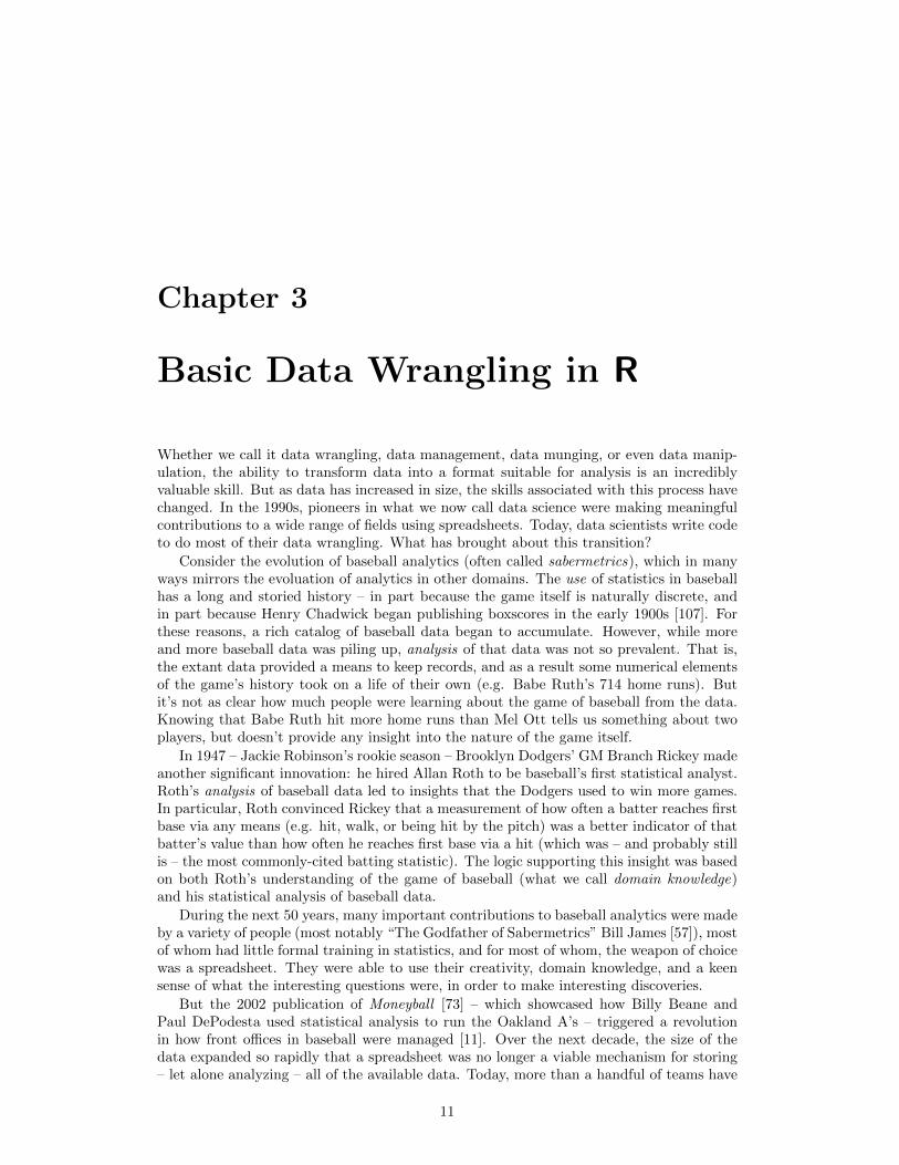
The two most commonly used of the five idioms are filter and select, which allow youto return only a subset of the rows or columns of a data frame, respectively.
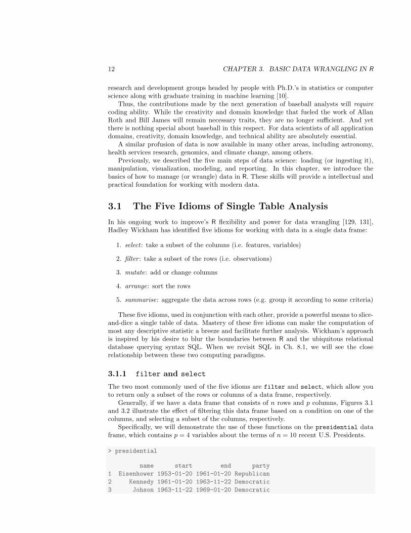
Generally, if we have a data frame that consists of n rows and p columns, Figures 3.1and 3.2 illustrate the effect of filtering this data frame based on a condition on one of thecolumns, and selecting a subset of the columns, respectively.
Specifically, we will demonstrate the use of these functions on the presidential dataframe, which contains p = 4 variables about the terms of n = 10 recent U.S. Presidents.
> presidential
name start end party
1 Eisenhower 1953-01-20 1961-01-20 Republican
2 Kennedy 1961-01-20 1963-11-22 Democratic
3 Johson 1963-11-22 1969-01-20 Democratic
3.1. THE FIVE IDIOMS OF SINGLE TABLE ANALYSIS 13
n
k
m ≤ n
k
Figure 3.1: filter. At left, a data frame that contains matching entries in a certain columnfor only a subset of the rows. At right, the resulting data frame after filtering.
n
k
n
� ≤ k
Figure 3.2: select. At left, a data frame, from which we retrieve only a few of the columns.At right, the resulting data frame after selecting those columns.
4 Nixon 1969-01-20 1974-08-09 Republican
5 Ford 1974-08-09 1977-01-20 Republican
6 Carter 1977-01-20 1981-01-20 Democratic
7 Reagan 1981-01-20 1989-01-20 Republican
8 Bush 1989-01-20 1993-01-20 Republican
9 Clinton 1993-01-20 2001-01-20 Democratic
10 Bush 2001-01-20 2009-01-20 Republican
To retrieve only the names and party affiliations of these presidents, we would useselect. The first argument to the select function is the data frame, followed by anarbitrarily long list of column names, separated by commas. Note that it is not necessaryto wrap the column names in quotation marks.
> select(presidential, name, party)
name party
1 Eisenhower Republican
2 Kennedy Democratic
3 Johson Democratic
4 Nixon Republican
5 Ford Republican
6 Carter Democratic
7 Reagan Republican
8 Bush Republican
9 Clinton Democratic
10 Bush Republican
14 CHAPTER 3. BASIC DATA WRANGLING IN R
Similarly, the first argument to filter is a data frame, and subsequent arguments arelogical conditions that are evaluated on any involved columns. Thus, if we want to retrieveonly those rows that pertain to Republican presidents, we need to specify that the value ofthe party variable is equal to Republican.
> filter(presidential, party == "Republican")
name start end party
1 Eisenhower 1953-01-20 1961-01-20 Republican
2 Nixon 1969-01-20 1974-08-09 Republican
3 Ford 1974-08-09 1977-01-20 Republican
4 Reagan 1981-01-20 1989-01-20 Republican
5 Bush 1989-01-20 1993-01-20 Republican
6 Bush 2001-01-20 2009-01-20 Republican
Note that the == is a test for equality. If we were to use only a single equal sign here,we would be asserting that party = "Republican". This would cause all of the rows ofpresidential to be returned, since we would have overwritten the actual values of theparty variable. Note also the the quotation marks around "Republican" are necessaryhere, since "Republican" is a literal value, and not a variable name.
Naturally, combining filter and select commands enable one to drill down to veryspecific pieces of information. For example, we can find which Democratic presidents servedsince Watergate.
> select(filter(presidential, start > 1973 & party == "Democratic"), name)
name
1 Carter
2 Clinton
The same output could be generated using the %>%) (pipe) operator. Pipe-forwarding isan alternative to nesting that yields code that can be read from top to bottom.
> presidential %>%
filter(start > 1973 & party == "Democratic") %>%
select(name)
name
1 Carter
2 Clinton
In later chapters we will see how this operator can make our code more efficient, partic-ularly for complex operations on large datasets.
3.1.2 mutate and rename
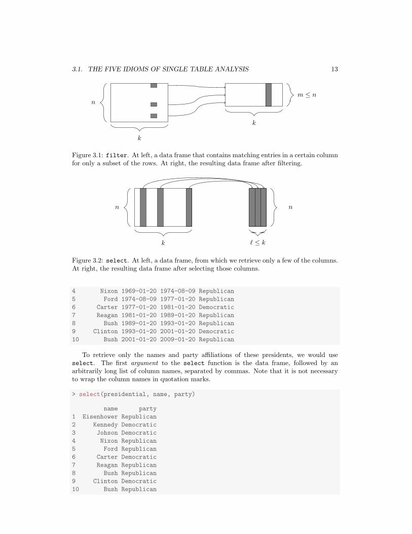
Frequently, in the process of conducting our analysis, we will create, re-define, and renamesome of our variables. The functions mutate and rename provide these capabilities. Anillustration of mutate is shown in Figure 3.3.
While we have the raw data on when each of these presidents took and relinquishedoffice, we don’t actually have a numeric variable giving the length of each president’s term.Of course, we can derive this information from the dates given, and add the result as a
3.1. THE FIVE IDIOMS OF SINGLE TABLE ANALYSIS 15
n
k
n
k + 1
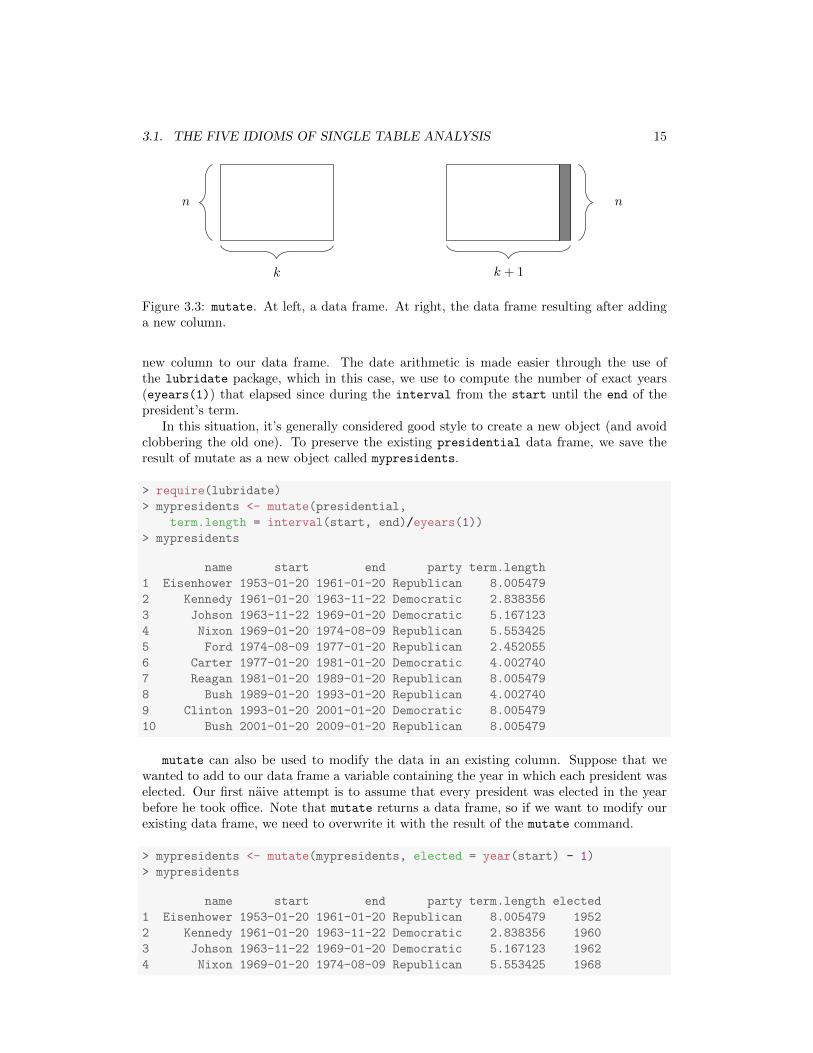
Figure 3.3: mutate. At left, a data frame. At right, the data frame resulting after addinga new column.
new column to our data frame. The date arithmetic is made easier through the use ofthe lubridate package, which in this case, we use to compute the number of exact years(eyears(1)) that elapsed since during the interval from the start until the end of thepresident’s term.
In this situation, it’s generally considered good style to create a new object (and avoidclobbering the old one). To preserve the existing presidential data frame, we save theresult of mutate as a new object called mypresidents.
> require(lubridate)
> mypresidents <- mutate(presidential,
term.length = interval(start, end)/eyears(1))
> mypresidents
name start end party term.length
1 Eisenhower 1953-01-20 1961-01-20 Republican 8.005479
2 Kennedy 1961-01-20 1963-11-22 Democratic 2.838356
3 Johson 1963-11-22 1969-01-20 Democratic 5.167123
4 Nixon 1969-01-20 1974-08-09 Republican 5.553425
5 Ford 1974-08-09 1977-01-20 Republican 2.452055
6 Carter 1977-01-20 1981-01-20 Democratic 4.002740
7 Reagan 1981-01-20 1989-01-20 Republican 8.005479
8 Bush 1989-01-20 1993-01-20 Republican 4.002740
9 Clinton 1993-01-20 2001-01-20 Democratic 8.005479
10 Bush 2001-01-20 2009-01-20 Republican 8.005479
mutate can also be used to modify the data in an existing column. Suppose that wewanted to add to our data frame a variable containing the year in which each president waselected. Our first naive attempt is to assume that every president was elected in the yearbefore he took office. Note that mutate returns a data frame, so if we want to modify ourexisting data frame, we need to overwrite it with the result of the mutate command.
> mypresidents <- mutate(mypresidents, elected = year(start) - 1)
> mypresidents
name start end party term.length elected
1 Eisenhower 1953-01-20 1961-01-20 Republican 8.005479 1952
2 Kennedy 1961-01-20 1963-11-22 Democratic 2.838356 1960
3 Johson 1963-11-22 1969-01-20 Democratic 5.167123 1962
4 Nixon 1969-01-20 1974-08-09 Republican 5.553425 1968
16 CHAPTER 3. BASIC DATA WRANGLING IN R
5 Ford 1974-08-09 1977-01-20 Republican 2.452055 1973
6 Carter 1977-01-20 1981-01-20 Democratic 4.002740 1976
7 Reagan 1981-01-20 1989-01-20 Republican 8.005479 1980
8 Bush 1989-01-20 1993-01-20 Republican 4.002740 1988
9 Clinton 1993-01-20 2001-01-20 Democratic 8.005479 1992
10 Bush 2001-01-20 2009-01-20 Republican 8.005479 2000
Some aspects of this dataset are wrong, because presidential elections are only held everyfour years. Lyndon Johnson assumed the office after President Kennedy was assassinatedin 1963, and Gerald Ford took over after President Nixon resigned in 1974. Thus, therewere no presidential elections in 1962 or 1973, as suggested in our data frame. We shouldoverwrite these values with NA’s. We can use the ifelse function to do this.
> mypresidents <- mutate(mypresidents,
elected = ifelse((elected %in% c(1962, 1973)), NA, elected))
> mypresidents
name start end party term.length elected
1 Eisenhower 1953-01-20 1961-01-20 Republican 8.005479 1952
2 Kennedy 1961-01-20 1963-11-22 Democratic 2.838356 1960
3 Johson 1963-11-22 1969-01-20 Democratic 5.167123 NA
4 Nixon 1969-01-20 1974-08-09 Republican 5.553425 1968
5 Ford 1974-08-09 1977-01-20 Republican 2.452055 NA
6 Carter 1977-01-20 1981-01-20 Democratic 4.002740 1976
7 Reagan 1981-01-20 1989-01-20 Republican 8.005479 1980
8 Bush 1989-01-20 1993-01-20 Republican 4.002740 1988
9 Clinton 1993-01-20 2001-01-20 Democratic 8.005479 1992
10 Bush 2001-01-20 2009-01-20 Republican 8.005479 2000
Here, if the value of elected is either 1962 or 1973, we overwrite that value with NA 1.Otherwise, we overwrite it with the same value that it currently has.
Finally, it is considered bad practice to use periods in the name of functions, data frames,and variables in R. Ill-advised periods could conflict with R’s use of generic functions (i.e. R’smechanism for method overloading). Thus, we should change the name of the term.lengthcolumn that we created earlier. In this book, we will use camelCase for function and variablenames.
Pro Tip 1 Don’t use periods in the names of functions, data frames, and variables.
> mypresidents <- rename(mypresidents, termLength = term.length)
> mypresidents
name start end party termLength elected
1 Eisenhower 1953-01-20 1961-01-20 Republican 8.005479 1952
2 Kennedy 1961-01-20 1963-11-22 Democratic 2.838356 1960
3 Johson 1963-11-22 1969-01-20 Democratic 5.167123 NA
4 Nixon 1969-01-20 1974-08-09 Republican 5.553425 1968
5 Ford 1974-08-09 1977-01-20 Republican 2.452055 NA
6 Carter 1977-01-20 1981-01-20 Democratic 4.002740 1976
1Incidentally, Johnson was elected in 1964 as an incumbent.
3.1. THE FIVE IDIOMS OF SINGLE TABLE ANALYSIS 17
n
k
n
k
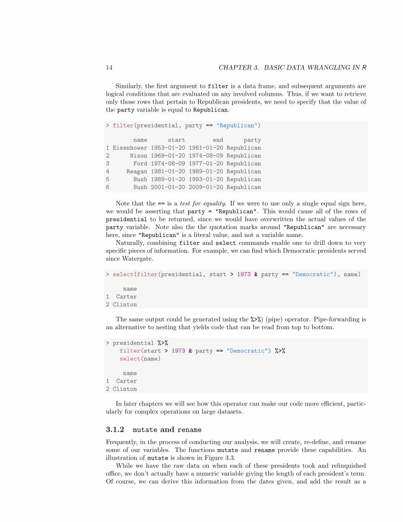
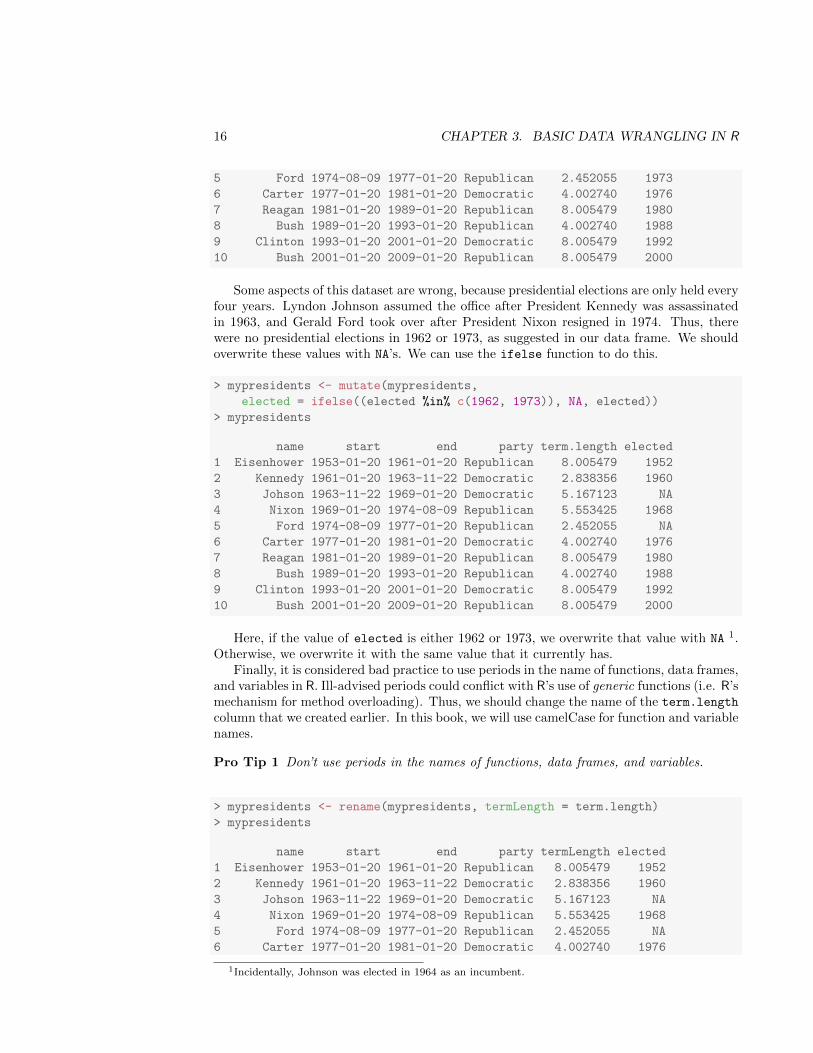
Figure 3.4: arrange. At left, a data frame with an ordinal variable. At right, the resultingdata frame after sorting the rows in descending order of that variable.
7 Reagan 1981-01-20 1989-01-20 Republican 8.005479 1980
8 Bush 1989-01-20 1993-01-20 Republican 4.002740 1988
9 Clinton 1993-01-20 2001-01-20 Democratic 8.005479 1992
10 Bush 2001-01-20 2009-01-20 Republican 8.005479 2000
3.1.3 arrange
It’s tempting to think that the function sort will sort a data frame in R—but that doesn’twork. There is a function called sort, and it does exactly what you think it does, butit works on vectors, not data frames. The function that will sort a data frame is calledarrange. It’s functionality is illustrated in Figure 3.4.
In order to arrange a data frame, you have to specify the data frame, and the columnby which you want it to be sorted. You also have to specify the direction in which you wantit to be sorted. Specifying multiple sort conditions will results in ties being broken.
Thus, to sort our presidential data frame by the length of each president’s term, wespecify that we want the column termLength in descending order.
> arrange(mypresidents, desc(termLength))
name start end party termLength elected
1 Eisenhower 1953-01-20 1961-01-20 Republican 8.005479 1952
2 Reagan 1981-01-20 1989-01-20 Republican 8.005479 1980
3 Clinton 1993-01-20 2001-01-20 Democratic 8.005479 1992
4 Bush 2001-01-20 2009-01-20 Republican 8.005479 2000
5 Nixon 1969-01-20 1974-08-09 Republican 5.553425 1968
6 Johson 1963-11-22 1969-01-20 Democratic 5.167123 NA
7 Carter 1977-01-20 1981-01-20 Democratic 4.002740 1976
8 Bush 1989-01-20 1993-01-20 Republican 4.002740 1988
9 Kennedy 1961-01-20 1963-11-22 Democratic 2.838356 1960
10 Ford 1974-08-09 1977-01-20 Republican 2.452055 NA
A number of presidents completed both one and two full terms, and thus have the exactsame term length. We can futher sort by party and elected.
> arrange(mypresidents, desc(termLength), party, elected)
name start end party termLength elected
1 Clinton 1993-01-20 2001-01-20 Democratic 8.005479 1992
18 CHAPTER 3. BASIC DATA WRANGLING IN R
n
k
1
� ≤ k
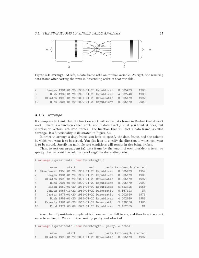
Figure 3.5: summarise. At left, a data frame. At right, the resulting data frame afteraggregating three of the columns.
2 Eisenhower 1953-01-20 1961-01-20 Republican 8.005479 1952
3 Reagan 1981-01-20 1989-01-20 Republican 8.005479 1980
4 Bush 2001-01-20 2009-01-20 Republican 8.005479 2000
5 Nixon 1969-01-20 1974-08-09 Republican 5.553425 1968
6 Johson 1963-11-22 1969-01-20 Democratic 5.167123 NA
7 Carter 1977-01-20 1981-01-20 Democratic 4.002740 1976
8 Bush 1989-01-20 1993-01-20 Republican 4.002740 1988
9 Kennedy 1961-01-20 1963-11-22 Democratic 2.838356 1960
10 Ford 1974-08-09 1977-01-20 Republican 2.452055 NA
Note that the default sort order is ascending order, so we do not need to specify that ifthat is what we want.
3.1.4 summarise with group by
Our last of the five idioms for single-table analysis is summarise, which is nearly alwaysused in conjunction with group by. The previous four idioms provided us with means tomanipulate a data frame in powerful and flexible ways. But the extent of the analysis wecan perform with these four idioms alone is limited. On the other hand, summarise withgroup by enables us to make comparisons.
When used alone, summarise collapses a data frame into a single row. This is illustratedin Figure 3.5. Critically, we have to specify how we want to reduce an entire column of datainto a single value. The method of aggregation that we specify controls what will appearin the output.
> summarise(mypresidents, numPresidents = n()
, firstYear = min(year(start)), lastYear = max(year(end))
, numDemocrats = sum(party == "Democratic")
, tTermLength = sum(termLength), mTermLength = mean(termLength))
numPresidents firstYear lastYear numDemocrats tTermLength mTermLength
1 10 1953 2009 4 56.03836 5.603836
Once again, the first argument to summarise is a data frame, followed by a list ofcolumns that will appear in the output. Note that every column in the output is defined byoperations performed on vectors – not on individual values. This is essential, since if thespecification of an output column is not an operation on a vector, there is no way for R toknow how to collapse each column.
3.2. EXTENDED EXAMPLE: BEN’S TIME WITH THE METS 19
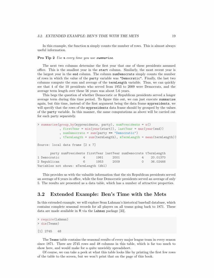
In this example, the function n simply counts the number of rows. This is almost alwaysuseful information.
Pro Tip 2 Use n every time you use summarise.
The next two columns determine the first year that one of these presidents assumedoffice. This is the smallest year in the start column. Similarly, the most recent year isthe largest year in the end column. The column numDemocrats simply counts the numberof rows in which the value of the party variable was "Democratic". Finally, the last twocolumns compute the sum and average of the termLength variable. Thus, we can quicklysee that 4 of the 10 presidents who served from 1953 to 2009 were Democrats, and theaverage term length over these 56 years was about 5.6 years.
This begs the question of whether Democratic or Republican presidents served a longeraverage term during this time period. To figure this out, we can just execute summarise
again, but this time, instead of the first argument being the data frame mypresidents, wewill specify that the rows of the mypresidents data frame should by grouped by the valuesof the party variable. In this manner, the same computations as above will be carried outfor each party separately.
> summarise(group_by(mypresidents, party), numPresidents = n()
, firstYear = min(year(start)), lastYear = max(year(end))
, numDemocrats = sum(party == "Democratic")
, tTermLength = sum(termLength), mTermLength = mean(termLength))
Source: local data frame [2 x 7]
party numPresidents firstYear lastYear numDemocrats tTermLength
1 Democratic 4 1961 2001 4 20.01370
2 Republican 6 1953 2009 0 36.02466
Variables not shown: mTermLength (dbl)
This provides us with the valuable information that the six Republican presidents servedan average of 6 years in office, while the four Democratic presidents served an average of only5. The results are presented as a data table, which has a number of attractive properties.
3.2 Extended Example: Ben’s Time with the Mets
In this extended example, we will explore Sean Lahman’s historical baseball database, whichcontains complete seasonal records for all players on all teams going back to 1871. Thesedata are made available in R via the Lahman package [33].
> require(Lahman)
> dim(Teams)
[1] 2745 48
The Teams table contains the seasonal results of every major league team in every seasonsince 1871. There are 2745 rows and 48 columns in this table, which is far too much toshow here, and would make for a quite unwieldy spreadsheet.
Of course, we can take a peek at what this table looks like by printing the first few rowsof the table to the screen, but we won’t print that on the page of this book.
20 CHAPTER 3. BASIC DATA WRANGLING IN R
> head(Teams)
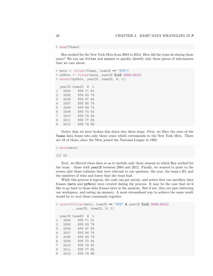
Ben worked for the New York Mets from 2004 to 2012. How did the team do during thoseyears? We can use filter and select to quickly identify only those pieces of informationthat we care about.
> mets <- filter(Teams, teamID == "NYN")
> myMets <- filter(mets, yearID %in% 2004:2012)
> select(myMets, yearID, teamID, W, L)
yearID teamID W L
1 2004 NYN 71 91
2 2005 NYN 83 79
3 2006 NYN 97 65
4 2007 NYN 88 74
5 2008 NYN 89 73
6 2009 NYN 70 92
7 2010 NYN 79 83
8 2011 NYN 77 85
9 2012 NYN 74 88
Notice that we have broken this down into three steps. First, we filter the rows of theTeams data frame into only those years which corresponds to the New York Mets. Thereare 52 of those, since the Mets joined the National League in 1962.
> nrow(mets)
[1] 52
Next, we filtered these data so as to include only those seasons in which Ben worked forthe team – those with yearID between 2004 and 2012. Finally, we wanted to print to thescreen only those columns that were relevant to our question: the year, the team’s ID, andthe numbers of wins and losses that the team had.
While this process is logical, the code can get unruly, and notice that two ancillary dataframes (mets and myMets) were created during the process. It may be the case that we’dlike to go back to those data frames later in the analysis. But if not, they are just clutteringour workspace, and eating up memory. A more streamlined way to achieve the same resultwould be to nest these commands together.
> select(filter(mets, teamID == "NYN" & yearID %in% 2004:2012)
, yearID, teamID, W, L)
yearID teamID W L
1 2004 NYN 71 91
2 2005 NYN 83 79
3 2006 NYN 97 65
4 2007 NYN 88 74
5 2008 NYN 89 73
6 2009 NYN 70 92
7 2010 NYN 79 83
8 2011 NYN 77 85
9 2012 NYN 74 88
3.2. EXTENDED EXAMPLE: BEN’S TIME WITH THE METS 21
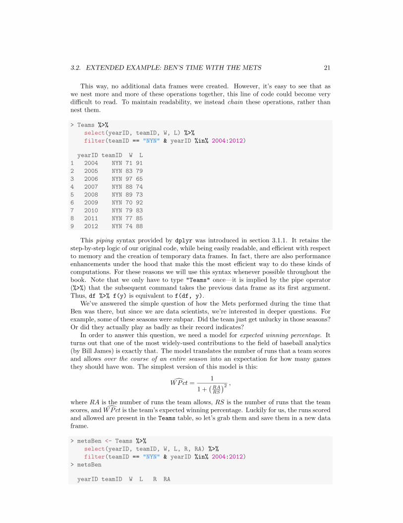
This way, no additional data frames were created. However, it’s easy to see that aswe nest more and more of these operations together, this line of code could become verydifficult to read. To maintain readability, we instead chain these operations, rather thannest them.
> Teams %>%
select(yearID, teamID, W, L) %>%
filter(teamID == "NYN" & yearID %in% 2004:2012)
yearID teamID W L
1 2004 NYN 71 91
2 2005 NYN 83 79
3 2006 NYN 97 65
4 2007 NYN 88 74
5 2008 NYN 89 73
6 2009 NYN 70 92
7 2010 NYN 79 83
8 2011 NYN 77 85
9 2012 NYN 74 88
This piping syntax provided by dplyr was introduced in section 3.1.1. It retains thestep-by-step logic of our original code, while being easily readable, and efficient with respectto memory and the creation of temporary data frames. In fact, there are also performanceenhancements under the hood that make this the most efficient way to do these kinds ofcomputations. For these reasons we will use this syntax whenever possible throughout thebook. Note that we only have to type "Teams" once—it is implied by the pipe operator(%>%) that the subsequent command takes the previous data frame as its first argument.Thus, df %>% f(y) is equivalent to f(df, y).
We’ve answered the simple question of how the Mets performed during the time thatBen was there, but since we are data scientists, we’re interested in deeper questions. Forexample, some of these seasons were subpar. Did the team just get unlucky in those seasons?Or did they actually play as badly as their record indicates?
In order to answer this question, we need a model for expected winning percentage. Itturns out that one of the most widely-used contributions to the field of baseball analytics(by Bill James) is exactly that. The model translates the number of runs that a team scoresand allows over the course of an entire season into an expectation for how many gamesthey should have won. The simplest version of this model is this:
�WPct =1
1 +�RARS
�2 ,
where RA is the number of runs the team allows, RS is the number of runs that the teamscores, and �WPct is the team’s expected winning percentage. Luckily for us, the runs scoredand allowed are present in the Teams table, so let’s grab them and save them in a new dataframe.
> metsBen <- Teams %>%
select(yearID, teamID, W, L, R, RA) %>%
filter(teamID == "NYN" & yearID %in% 2004:2012)
> metsBen
yearID teamID W L R RA
22 CHAPTER 3. BASIC DATA WRANGLING IN R
1 2004 NYN 71 91 684 731
2 2005 NYN 83 79 722 648
3 2006 NYN 97 65 834 731
4 2007 NYN 88 74 804 750
5 2008 NYN 89 73 799 715
6 2009 NYN 70 92 671 757
7 2010 NYN 79 83 656 652
8 2011 NYN 77 85 718 742
9 2012 NYN 74 88 650 709
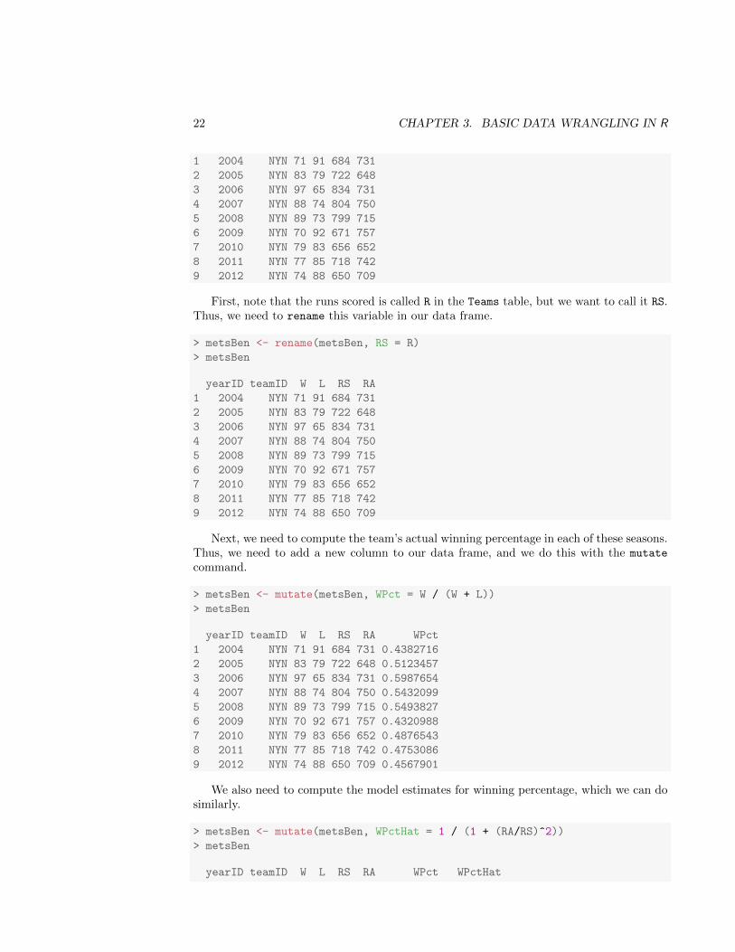
First, note that the runs scored is called R in the Teams table, but we want to call it RS.Thus, we need to rename this variable in our data frame.
> metsBen <- rename(metsBen, RS = R)
> metsBen
yearID teamID W L RS RA
1 2004 NYN 71 91 684 731
2 2005 NYN 83 79 722 648
3 2006 NYN 97 65 834 731
4 2007 NYN 88 74 804 750
5 2008 NYN 89 73 799 715
6 2009 NYN 70 92 671 757
7 2010 NYN 79 83 656 652
8 2011 NYN 77 85 718 742
9 2012 NYN 74 88 650 709
Next, we need to compute the team’s actual winning percentage in each of these seasons.Thus, we need to add a new column to our data frame, and we do this with the mutate
command.
> metsBen <- mutate(metsBen, WPct = W / (W + L))
> metsBen
yearID teamID W L RS RA WPct
1 2004 NYN 71 91 684 731 0.4382716
2 2005 NYN 83 79 722 648 0.5123457
3 2006 NYN 97 65 834 731 0.5987654
4 2007 NYN 88 74 804 750 0.5432099
5 2008 NYN 89 73 799 715 0.5493827
6 2009 NYN 70 92 671 757 0.4320988
7 2010 NYN 79 83 656 652 0.4876543
8 2011 NYN 77 85 718 742 0.4753086
9 2012 NYN 74 88 650 709 0.4567901
We also need to compute the model estimates for winning percentage, which we can dosimilarly.
> metsBen <- mutate(metsBen, WPctHat = 1 / (1 + (RA/RS)^2))
> metsBen
yearID teamID W L RS RA WPct WPctHat
3.2. EXTENDED EXAMPLE: BEN’S TIME WITH THE METS 23
1 2004 NYN 71 91 684 731 0.4382716 0.4668211
2 2005 NYN 83 79 722 648 0.5123457 0.5538575
3 2006 NYN 97 65 834 731 0.5987654 0.5655308
4 2007 NYN 88 74 804 750 0.5432099 0.5347071
5 2008 NYN 89 73 799 715 0.5493827 0.5553119
6 2009 NYN 70 92 671 757 0.4320988 0.4399936
7 2010 NYN 79 83 656 652 0.4876543 0.5030581
8 2011 NYN 77 85 718 742 0.4753086 0.4835661
9 2012 NYN 74 88 650 709 0.4567901 0.4566674
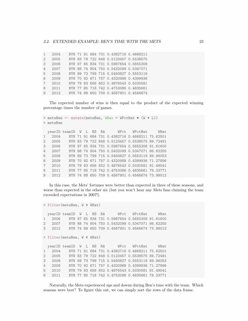
The expected number of wins is then equal to the product of the expected winningpercentage times the number of games.
> metsBen <- mutate(metsBen, WHat = WPctHat * (W + L))
> metsBen
yearID teamID W L RS RA WPct WPctHat WHat
1 2004 NYN 71 91 684 731 0.4382716 0.4668211 75.62501
2 2005 NYN 83 79 722 648 0.5123457 0.5538575 89.72491
3 2006 NYN 97 65 834 731 0.5987654 0.5655308 91.61600
4 2007 NYN 88 74 804 750 0.5432099 0.5347071 86.62255
5 2008 NYN 89 73 799 715 0.5493827 0.5553119 89.96053
6 2009 NYN 70 92 671 757 0.4320988 0.4399936 71.27896
7 2010 NYN 79 83 656 652 0.4876543 0.5030581 81.49541
8 2011 NYN 77 85 718 742 0.4753086 0.4835661 78.33771
9 2012 NYN 74 88 650 709 0.4567901 0.4566674 73.98012
In this case, the Mets’ fortunes were better than expected in three of these seasons, andworse than expected in the other six (but you won’t hear any Mets fans claiming the teamexceeded expectations in 2007!).
> filter(metsBen, W > WHat)
yearID teamID W L RS RA WPct WPctHat WHat
1 2006 NYN 97 65 834 731 0.5987654 0.5655308 91.61600
2 2007 NYN 88 74 804 750 0.5432099 0.5347071 86.62255
3 2012 NYN 74 88 650 709 0.4567901 0.4566674 73.98012
> filter(metsBen, W < WHat)
yearID teamID W L RS RA WPct WPctHat WHat
1 2004 NYN 71 91 684 731 0.4382716 0.4668211 75.62501
2 2005 NYN 83 79 722 648 0.5123457 0.5538575 89.72491
3 2008 NYN 89 73 799 715 0.5493827 0.5553119 89.96053
4 2009 NYN 70 92 671 757 0.4320988 0.4399936 71.27896
5 2010 NYN 79 83 656 652 0.4876543 0.5030581 81.49541
6 2011 NYN 77 85 718 742 0.4753086 0.4835661 78.33771
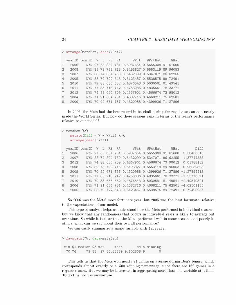
Naturally, the Mets experienced ups and downs during Ben’s time with the team. Whichseasons were best? To figure this out, we can simply sort the rows of the data frame.
24 CHAPTER 3. BASIC DATA WRANGLING IN R
> arrange(metsBen, desc(WPct))
yearID teamID W L RS RA WPct WPctHat WHat
1 2006 NYN 97 65 834 731 0.5987654 0.5655308 91.61600
2 2008 NYN 89 73 799 715 0.5493827 0.5553119 89.96053
3 2007 NYN 88 74 804 750 0.5432099 0.5347071 86.62255
4 2005 NYN 83 79 722 648 0.5123457 0.5538575 89.72491
5 2010 NYN 79 83 656 652 0.4876543 0.5030581 81.49541
6 2011 NYN 77 85 718 742 0.4753086 0.4835661 78.33771
7 2012 NYN 74 88 650 709 0.4567901 0.4566674 73.98012
8 2004 NYN 71 91 684 731 0.4382716 0.4668211 75.62501
9 2009 NYN 70 92 671 757 0.4320988 0.4399936 71.27896
In 2006, the Mets had the best record in baseball during the regular season and nearlymade the World Series. But how do these seasons rank in terms of the team’s performancerelative to our model?
> metsBen %>%
mutate(Diff = W - WHat) %>%
arrange(desc(Diff))
yearID teamID W L RS RA WPct WPctHat WHat Diff
1 2006 NYN 97 65 834 731 0.5987654 0.5655308 91.61600 5.38400315
2 2007 NYN 88 74 804 750 0.5432099 0.5347071 86.62255 1.37744558
3 2012 NYN 74 88 650 709 0.4567901 0.4566674 73.98012 0.01988152
4 2008 NYN 89 73 799 715 0.5493827 0.5553119 89.96053 -0.96052803
5 2009 NYN 70 92 671 757 0.4320988 0.4399936 71.27896 -1.27895513
6 2011 NYN 77 85 718 742 0.4753086 0.4835661 78.33771 -1.33770571
7 2010 NYN 79 83 656 652 0.4876543 0.5030581 81.49541 -2.49540821
8 2004 NYN 71 91 684 731 0.4382716 0.4668211 75.62501 -4.62501135
9 2005 NYN 83 79 722 648 0.5123457 0.5538575 89.72491 -6.72490937
So 2006 was the Mets’ most fortunate year, but 2005 was the least fortunate, relativeto the expectations of our model.
This type of analysis helps us understand how the Mets performed in individual seasons,but we know that any randomness that occurs in individual years is likely to average outover time. So while it is clear that the Mets performed well in some seasons and poorly inothers, what can we say about their overall performance?
We can easily summarize a single variable with favstats.
> favstats(~W, data=metsBen)
min Q1 median Q3 max mean sd n missing
70 74 79 88 97 80.88889 9.102808 9 0
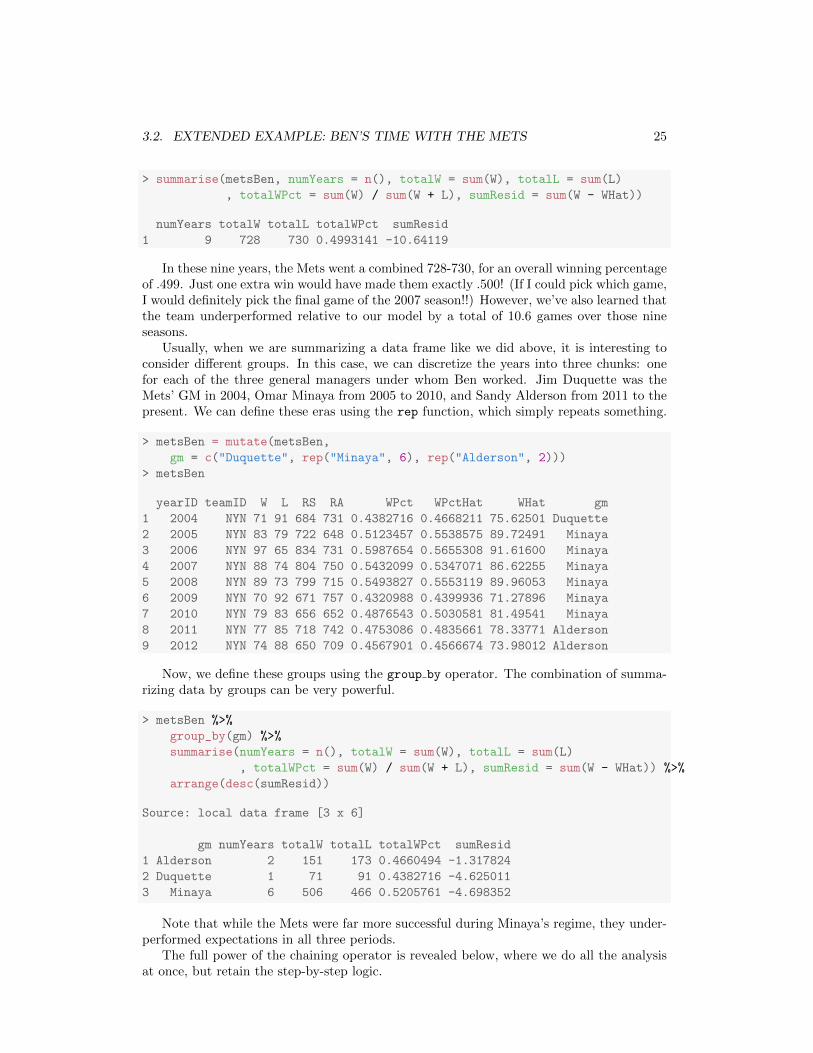
This tells us that the Mets won nearly 81 games on average during Ben’s tenure, whichcorresponds almost exactly to a .500 winning percentage, since there are 162 games in aregular season. But we may be interested in aggregating more than one variable at a time.To do this, we use summarise.
3.2. EXTENDED EXAMPLE: BEN’S TIME WITH THE METS 25
> summarise(metsBen, numYears = n(), totalW = sum(W), totalL = sum(L)
, totalWPct = sum(W) / sum(W + L), sumResid = sum(W - WHat))
numYears totalW totalL totalWPct sumResid
1 9 728 730 0.4993141 -10.64119
In these nine years, the Mets went a combined 728-730, for an overall winning percentageof .499. Just one extra win would have made them exactly .500! (If I could pick which game,I would definitely pick the final game of the 2007 season!!) However, we’ve also learned thatthe team underperformed relative to our model by a total of 10.6 games over those nineseasons.
Usually, when we are summarizing a data frame like we did above, it is interesting toconsider different groups. In this case, we can discretize the years into three chunks: onefor each of the three general managers under whom Ben worked. Jim Duquette was theMets’ GM in 2004, Omar Minaya from 2005 to 2010, and Sandy Alderson from 2011 to thepresent. We can define these eras using the rep function, which simply repeats something.
> metsBen = mutate(metsBen,
gm = c("Duquette", rep("Minaya", 6), rep("Alderson", 2)))
> metsBen
yearID teamID W L RS RA WPct WPctHat WHat gm
1 2004 NYN 71 91 684 731 0.4382716 0.4668211 75.62501 Duquette
2 2005 NYN 83 79 722 648 0.5123457 0.5538575 89.72491 Minaya
3 2006 NYN 97 65 834 731 0.5987654 0.5655308 91.61600 Minaya
4 2007 NYN 88 74 804 750 0.5432099 0.5347071 86.62255 Minaya
5 2008 NYN 89 73 799 715 0.5493827 0.5553119 89.96053 Minaya
6 2009 NYN 70 92 671 757 0.4320988 0.4399936 71.27896 Minaya
7 2010 NYN 79 83 656 652 0.4876543 0.5030581 81.49541 Minaya
8 2011 NYN 77 85 718 742 0.4753086 0.4835661 78.33771 Alderson
9 2012 NYN 74 88 650 709 0.4567901 0.4566674 73.98012 Alderson
Now, we define these groups using the group by operator. The combination of summa-rizing data by groups can be very powerful.
> metsBen %>%
group_by(gm) %>%
summarise(numYears = n(), totalW = sum(W), totalL = sum(L)
, totalWPct = sum(W) / sum(W + L), sumResid = sum(W - WHat)) %>%
arrange(desc(sumResid))
Source: local data frame [3 x 6]
gm numYears totalW totalL totalWPct sumResid
1 Alderson 2 151 173 0.4660494 -1.317824
2 Duquette 1 71 91 0.4382716 -4.625011
3 Minaya 6 506 466 0.5205761 -4.698352
Note that while the Mets were far more successful during Minaya’s regime, they under-performed expectations in all three periods.
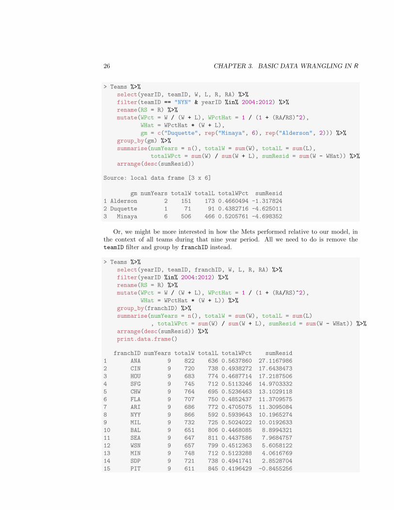
The full power of the chaining operator is revealed below, where we do all the analysisat once, but retain the step-by-step logic.
26 CHAPTER 3. BASIC DATA WRANGLING IN R
> Teams %>%
select(yearID, teamID, W, L, R, RA) %>%
filter(teamID == "NYN" & yearID %in% 2004:2012) %>%
rename(RS = R) %>%
mutate(WPct = W / (W + L), WPctHat = 1 / (1 + (RA/RS)^2),
WHat = WPctHat * (W + L),
gm = c("Duquette", rep("Minaya", 6), rep("Alderson", 2))) %>%
group_by(gm) %>%
summarise(numYears = n(), totalW = sum(W), totalL = sum(L),
totalWPct = sum(W) / sum(W + L), sumResid = sum(W - WHat)) %>%
arrange(desc(sumResid))
Source: local data frame [3 x 6]
gm numYears totalW totalL totalWPct sumResid
1 Alderson 2 151 173 0.4660494 -1.317824
2 Duquette 1 71 91 0.4382716 -4.625011
3 Minaya 6 506 466 0.5205761 -4.698352
Or, we might be more interested in how the Mets performed relative to our model, inthe context of all teams during that nine year period. All we need to do is remove theteamID filter and group by franchID instead.
> Teams %>%
select(yearID, teamID, franchID, W, L, R, RA) %>%
filter(yearID %in% 2004:2012) %>%
rename(RS = R) %>%
mutate(WPct = W / (W + L), WPctHat = 1 / (1 + (RA/RS)^2),
WHat = WPctHat * (W + L)) %>%
group_by(franchID) %>%
summarise(numYears = n(), totalW = sum(W), totalL = sum(L)
, totalWPct = sum(W) / sum(W + L), sumResid = sum(W - WHat)) %>%
arrange(desc(sumResid)) %>%
print.data.frame()
franchID numYears totalW totalL totalWPct sumResid
1 ANA 9 822 636 0.5637860 27.1167986
2 CIN 9 720 738 0.4938272 17.6438473
3 HOU 9 683 774 0.4687714 17.2187506
4 SFG 9 745 712 0.5113246 14.9703332
5 CHW 9 764 695 0.5236463 13.1029118
6 FLA 9 707 750 0.4852437 11.3709575
7 ARI 9 686 772 0.4705075 11.3095084
8 NYY 9 866 592 0.5939643 10.1965274
9 MIL 9 732 725 0.5024022 10.0192633
10 BAL 9 651 806 0.4468085 8.8994321
11 SEA 9 647 811 0.4437586 7.9684757
12 WSN 9 657 799 0.4512363 5.6058122
13 MIN 9 748 712 0.5123288 4.0616769
14 SDP 9 721 738 0.4941741 2.8528704
15 PIT 9 611 845 0.4196429 -0.8455256
3.3. COMBINING MULTIPLE TABLES 27
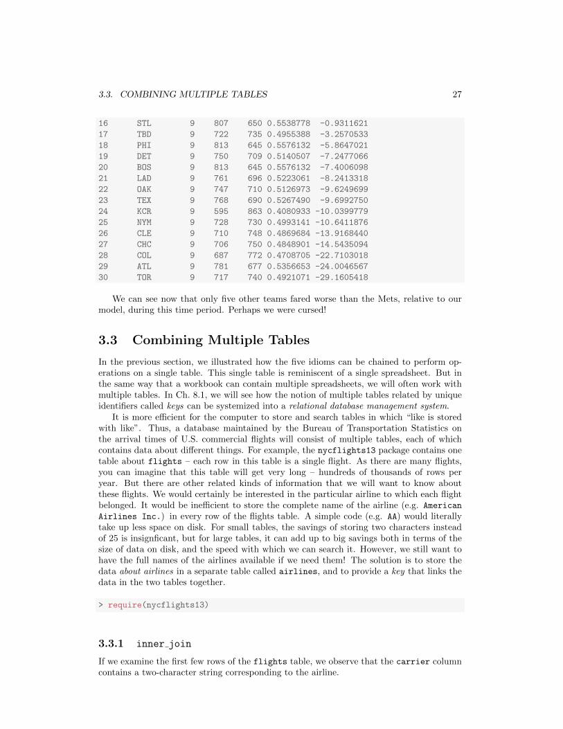
16 STL 9 807 650 0.5538778 -0.9311621
17 TBD 9 722 735 0.4955388 -3.2570533
18 PHI 9 813 645 0.5576132 -5.8647021
19 DET 9 750 709 0.5140507 -7.2477066
20 BOS 9 813 645 0.5576132 -7.4006098
21 LAD 9 761 696 0.5223061 -8.2413318
22 OAK 9 747 710 0.5126973 -9.6249699
23 TEX 9 768 690 0.5267490 -9.6992750
24 KCR 9 595 863 0.4080933 -10.0399779
25 NYM 9 728 730 0.4993141 -10.6411876
26 CLE 9 710 748 0.4869684 -13.9168440
27 CHC 9 706 750 0.4848901 -14.5435094
28 COL 9 687 772 0.4708705 -22.7103018
29 ATL 9 781 677 0.5356653 -24.0046567
30 TOR 9 717 740 0.4921071 -29.1605418
We can see now that only five other teams fared worse than the Mets, relative to ourmodel, during this time period. Perhaps we were cursed!
3.3 Combining Multiple Tables
In the previous section, we illustrated how the five idioms can be chained to perform op-erations on a single table. This single table is reminiscent of a single spreadsheet. But inthe same way that a workbook can contain multiple spreadsheets, we will often work withmultiple tables. In Ch. 8.1, we will see how the notion of multiple tables related by uniqueidentifiers called keys can be systemized into a relational database management system.
It is more efficient for the computer to store and search tables in which “like is storedwith like”. Thus, a database maintained by the Bureau of Transportation Statistics onthe arrival times of U.S. commercial flights will consist of multiple tables, each of whichcontains data about different things. For example, the nycflights13 package contains onetable about flights – each row in this table is a single flight. As there are many flights,you can imagine that this table will get very long – hundreds of thousands of rows peryear. But there are other related kinds of information that we will want to know aboutthese flights. We would certainly be interested in the particular airline to which each flightbelonged. It would be inefficient to store the complete name of the airline (e.g. American
Airlines Inc.) in every row of the flights table. A simple code (e.g. AA) would literallytake up less space on disk. For small tables, the savings of storing two characters insteadof 25 is insignficant, but for large tables, it can add up to big savings both in terms of thesize of data on disk, and the speed with which we can search it. However, we still want tohave the full names of the airlines available if we need them! The solution is to store thedata about airlines in a separate table called airlines, and to provide a key that links thedata in the two tables together.
> require(nycflights13)
3.3.1 inner join
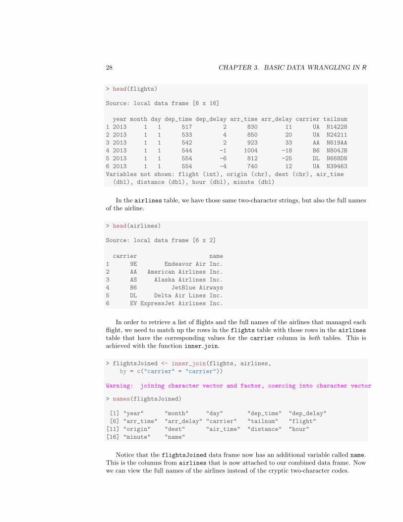
If we examine the first few rows of the flights table, we observe that the carrier columncontains a two-character string corresponding to the airline.
28 CHAPTER 3. BASIC DATA WRANGLING IN R
> head(flights)
Source: local data frame [6 x 16]
year month day dep_time dep_delay arr_time arr_delay carrier tailnum
1 2013 1 1 517 2 830 11 UA N14228
2 2013 1 1 533 4 850 20 UA N24211
3 2013 1 1 542 2 923 33 AA N619AA
4 2013 1 1 544 -1 1004 -18 B6 N804JB
5 2013 1 1 554 -6 812 -25 DL N668DN
6 2013 1 1 554 -4 740 12 UA N39463
Variables not shown: flight (int), origin (chr), dest (chr), air_time
(dbl), distance (dbl), hour (dbl), minute (dbl)
In the airlines table, we have those same two-character strings, but also the full namesof the airline.
> head(airlines)
Source: local data frame [6 x 2]
carrier name
1 9E Endeavor Air Inc.
2 AA American Airlines Inc.
3 AS Alaska Airlines Inc.
4 B6 JetBlue Airways
5 DL Delta Air Lines Inc.
6 EV ExpressJet Airlines Inc.
In order to retrieve a list of flights and the full names of the airlines that managed eachflight, we need to match up the rows in the flights table with those rows in the airlinestable that have the corresponding values for the carrier column in both tables. This isachieved with the function inner join.
> flightsJoined <- inner_join(flights, airlines,
by = c("carrier" = "carrier"))
Warning: joining character vector and factor, coercing into character vector
> names(flightsJoined)
[1] "year" "month" "day" "dep_time" "dep_delay"
[6] "arr_time" "arr_delay" "carrier" "tailnum" "flight"
[11] "origin" "dest" "air_time" "distance" "hour"
[16] "minute" "name"
Notice that the flightsJoined data frame now has an additional variable called name.This is the columns from airlines that is now attached to our combined data frame. Nowwe can view the full names of the airlines instead of the cryptic two-character codes.
3.3. COMBINING MULTIPLE TABLES 29
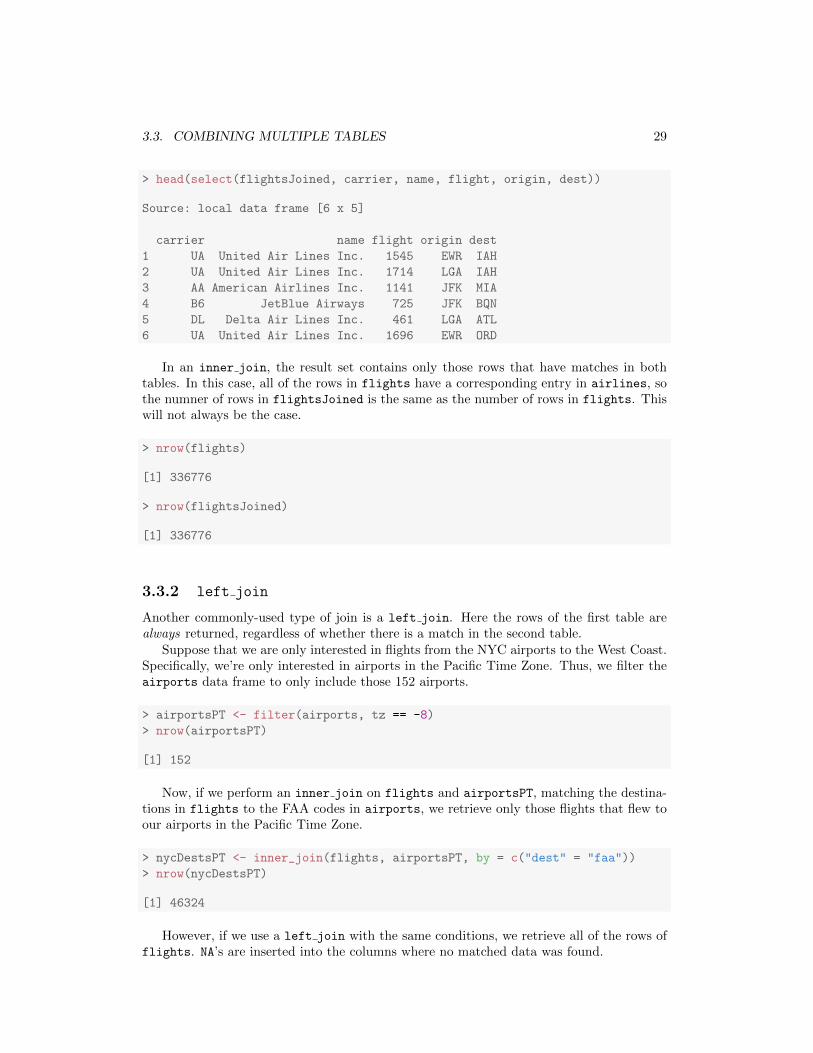
> head(select(flightsJoined, carrier, name, flight, origin, dest))
Source: local data frame [6 x 5]
carrier name flight origin dest
1 UA United Air Lines Inc. 1545 EWR IAH
2 UA United Air Lines Inc. 1714 LGA IAH
3 AA American Airlines Inc. 1141 JFK MIA
4 B6 JetBlue Airways 725 JFK BQN
5 DL Delta Air Lines Inc. 461 LGA ATL
6 UA United Air Lines Inc. 1696 EWR ORD
In an inner join, the result set contains only those rows that have matches in bothtables. In this case, all of the rows in flights have a corresponding entry in airlines, sothe numner of rows in flightsJoined is the same as the number of rows in flights. Thiswill not always be the case.
> nrow(flights)
[1] 336776
> nrow(flightsJoined)
[1] 336776
3.3.2 left join
Another commonly-used type of join is a left join. Here the rows of the first table arealways returned, regardless of whether there is a match in the second table.
Suppose that we are only interested in flights from the NYC airports to the West Coast.Specifically, we’re only interested in airports in the Pacific Time Zone. Thus, we filter theairports data frame to only include those 152 airports.
> airportsPT <- filter(airports, tz == -8)
> nrow(airportsPT)
[1] 152
Now, if we perform an inner join on flights and airportsPT, matching the destina-tions in flights to the FAA codes in airports, we retrieve only those flights that flew toour airports in the Pacific Time Zone.
> nycDestsPT <- inner_join(flights, airportsPT, by = c("dest" = "faa"))
> nrow(nycDestsPT)
[1] 46324
However, if we use a left join with the same conditions, we retrieve all of the rows offlights. NA’s are inserted into the columns where no matched data was found.
30 CHAPTER 3. BASIC DATA WRANGLING IN R
> nycDests <- left_join(flights, airportsPT, by = c("dest" = "faa"))
> nrow(nycDests)
[1] 336776
> sum(is.na(nycDests$name))
[1] 290452
Left joins can be extraordinarily useful in databases in which referential integrity isbroken (not all of the keys are present).
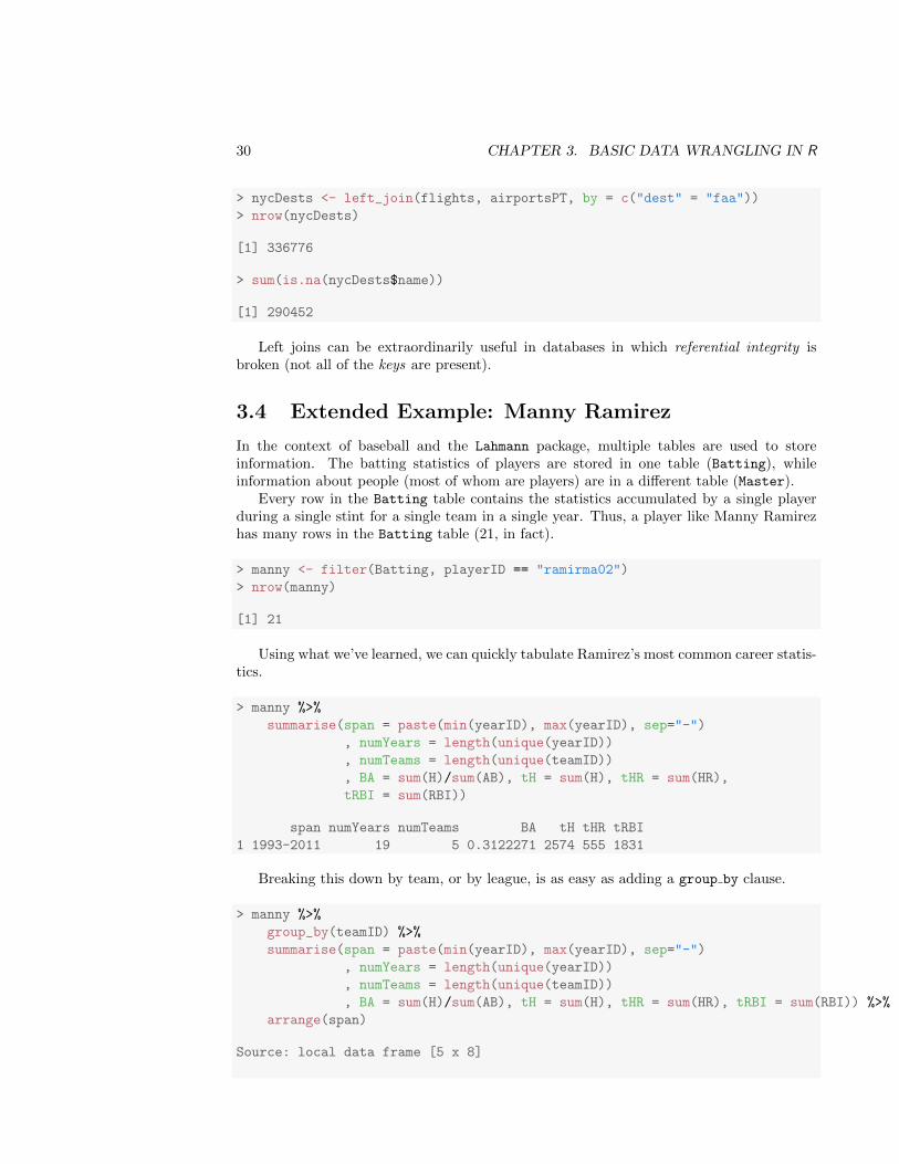
3.4 Extended Example: Manny Ramirez
In the context of baseball and the Lahmann package, multiple tables are used to storeinformation. The batting statistics of players are stored in one table (Batting), whileinformation about people (most of whom are players) are in a different table (Master).
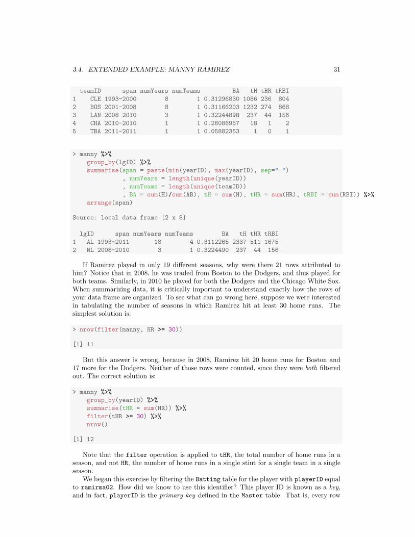
Every row in the Batting table contains the statistics accumulated by a single playerduring a single stint for a single team in a single year. Thus, a player like Manny Ramirezhas many rows in the Batting table (21, in fact).
> manny <- filter(Batting, playerID == "ramirma02")
> nrow(manny)
[1] 21
Using what we’ve learned, we can quickly tabulate Ramirez’s most common career statis-tics.
> manny %>%
summarise(span = paste(min(yearID), max(yearID), sep="-")
, numYears = length(unique(yearID))
, numTeams = length(unique(teamID))
, BA = sum(H)/sum(AB), tH = sum(H), tHR = sum(HR),
tRBI = sum(RBI))
span numYears numTeams BA tH tHR tRBI
1 1993-2011 19 5 0.3122271 2574 555 1831
Breaking this down by team, or by league, is as easy as adding a group by clause.
> manny %>%
group_by(teamID) %>%
summarise(span = paste(min(yearID), max(yearID), sep="-")
, numYears = length(unique(yearID))
, numTeams = length(unique(teamID))
, BA = sum(H)/sum(AB), tH = sum(H), tHR = sum(HR), tRBI = sum(RBI)) %>%
arrange(span)
Source: local data frame [5 x 8]
3.4. EXTENDED EXAMPLE: MANNY RAMIREZ 31
teamID span numYears numTeams BA tH tHR tRBI
1 CLE 1993-2000 8 1 0.31296830 1086 236 804
2 BOS 2001-2008 8 1 0.31166203 1232 274 868
3 LAN 2008-2010 3 1 0.32244898 237 44 156
4 CHA 2010-2010 1 1 0.26086957 18 1 2
5 TBA 2011-2011 1 1 0.05882353 1 0 1
> manny %>%
group_by(lgID) %>%
summarise(span = paste(min(yearID), max(yearID), sep="-")
, numYears = length(unique(yearID))
, numTeams = length(unique(teamID))
, BA = sum(H)/sum(AB), tH = sum(H), tHR = sum(HR), tRBI = sum(RBI)) %>%
arrange(span)
Source: local data frame [2 x 8]
lgID span numYears numTeams BA tH tHR tRBI
1 AL 1993-2011 18 4 0.3112265 2337 511 1675
2 NL 2008-2010 3 1 0.3224490 237 44 156
If Ramirez played in only 19 different seasons, why were there 21 rows attributed tohim? Notice that in 2008, he was traded from Boston to the Dodgers, and thus played forboth teams. Similarly, in 2010 he played for both the Dodgers and the Chicago White Sox.When summarizing data, it is critically important to understand exactly how the rows ofyour data frame are organized. To see what can go wrong here, suppose we were interestedin tabulating the number of seasons in which Ramirez hit at least 30 home runs. Thesimplest solution is:
> nrow(filter(manny, HR >= 30))
[1] 11
But this answer is wrong, because in 2008, Ramirez hit 20 home runs for Boston and17 more for the Dodgers. Neither of those rows were counted, since they were both filteredout. The correct solution is:
> manny %>%
group_by(yearID) %>%
summarise(tHR = sum(HR)) %>%
filter(tHR >= 30) %>%
nrow()
[1] 12
Note that the filter operation is applied to tHR, the total number of home runs in aseason, and not HR, the number of home runs in a single stint for a single team in a singleseason.
We began this exercise by filtering the Batting table for the player with playerID equalto ramirma02. How did we know to use this identifier? This player ID is known as a key,and in fact, playerID is the primary key defined in the Master table. That is, every row
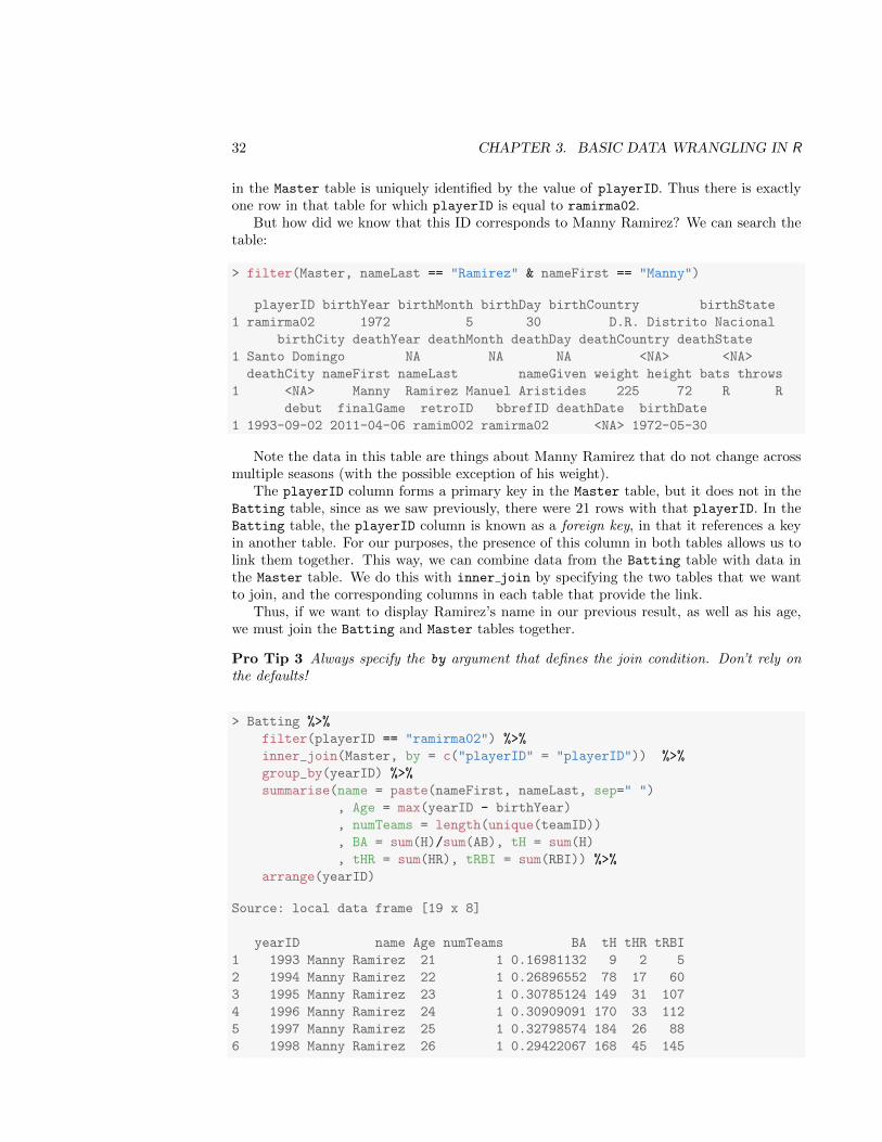
32 CHAPTER 3. BASIC DATA WRANGLING IN R
in the Master table is uniquely identified by the value of playerID. Thus there is exactlyone row in that table for which playerID is equal to ramirma02.
But how did we know that this ID corresponds to Manny Ramirez? We can search thetable:
> filter(Master, nameLast == "Ramirez" & nameFirst == "Manny")
playerID birthYear birthMonth birthDay birthCountry birthState
1 ramirma02 1972 5 30 D.R. Distrito Nacional
birthCity deathYear deathMonth deathDay deathCountry deathState
1 Santo Domingo NA NA NA <NA> <NA>
deathCity nameFirst nameLast nameGiven weight height bats throws
1 <NA> Manny Ramirez Manuel Aristides 225 72 R R
debut finalGame retroID bbrefID deathDate birthDate
1 1993-09-02 2011-04-06 ramim002 ramirma02 <NA> 1972-05-30
Note the data in this table are things about Manny Ramirez that do not change acrossmultiple seasons (with the possible exception of his weight).
The playerID column forms a primary key in the Master table, but it does not in theBatting table, since as we saw previously, there were 21 rows with that playerID. In theBatting table, the playerID column is known as a foreign key, in that it references a keyin another table. For our purposes, the presence of this column in both tables allows us tolink them together. This way, we can combine data from the Batting table with data inthe Master table. We do this with inner join by specifying the two tables that we wantto join, and the corresponding columns in each table that provide the link.
Thus, if we want to display Ramirez’s name in our previous result, as well as his age,we must join the Batting and Master tables together.
Pro Tip 3 Always specify the by argument that defines the join condition. Don’t rely onthe defaults!
> Batting %>%
filter(playerID == "ramirma02") %>%
inner_join(Master, by = c("playerID" = "playerID")) %>%
group_by(yearID) %>%
summarise(name = paste(nameFirst, nameLast, sep=" ")
, Age = max(yearID - birthYear)
, numTeams = length(unique(teamID))
, BA = sum(H)/sum(AB), tH = sum(H)
, tHR = sum(HR), tRBI = sum(RBI)) %>%
arrange(yearID)
Source: local data frame [19 x 8]
yearID name Age numTeams BA tH tHR tRBI
1 1993 Manny Ramirez 21 1 0.16981132 9 2 5
2 1994 Manny Ramirez 22 1 0.26896552 78 17 60
3 1995 Manny Ramirez 23 1 0.30785124 149 31 107
4 1996 Manny Ramirez 24 1 0.30909091 170 33 112
5 1997 Manny Ramirez 25 1 0.32798574 184 26 88
6 1998 Manny Ramirez 26 1 0.29422067 168 45 145
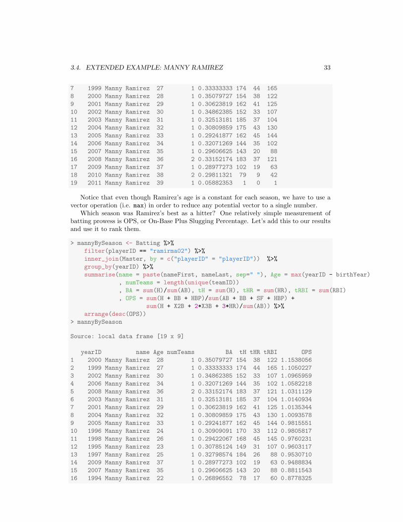
3.4. EXTENDED EXAMPLE: MANNY RAMIREZ 33
7 1999 Manny Ramirez 27 1 0.33333333 174 44 165
8 2000 Manny Ramirez 28 1 0.35079727 154 38 122
9 2001 Manny Ramirez 29 1 0.30623819 162 41 125
10 2002 Manny Ramirez 30 1 0.34862385 152 33 107
11 2003 Manny Ramirez 31 1 0.32513181 185 37 104
12 2004 Manny Ramirez 32 1 0.30809859 175 43 130
13 2005 Manny Ramirez 33 1 0.29241877 162 45 144
14 2006 Manny Ramirez 34 1 0.32071269 144 35 102
15 2007 Manny Ramirez 35 1 0.29606625 143 20 88
16 2008 Manny Ramirez 36 2 0.33152174 183 37 121
17 2009 Manny Ramirez 37 1 0.28977273 102 19 63
18 2010 Manny Ramirez 38 2 0.29811321 79 9 42
19 2011 Manny Ramirez 39 1 0.05882353 1 0 1
Notice that even though Ramirez’s age is a constant for each season, we have to use avector operation (i.e. max) in order to reduce any potential vector to a single number.
Which season was Ramirez’s best as a hitter? One relatively simple measurement ofbatting prowess is OPS, or On-Base Plus Slugging Percentage. Let’s add this to our resultsand use it to rank them.
> mannyBySeason <- Batting %>%
filter(playerID == "ramirma02") %>%
inner_join(Master, by = c("playerID" = "playerID")) %>%
group_by(yearID) %>%
summarise(name = paste(nameFirst, nameLast, sep=" "), Age = max(yearID - birthYear)
, numTeams = length(unique(teamID))
, BA = sum(H)/sum(AB), tH = sum(H), tHR = sum(HR), tRBI = sum(RBI)
, OPS = sum(H + BB + HBP)/sum(AB + BB + SF + HBP) +
sum(H + X2B + 2*X3B + 3*HR)/sum(AB)) %>%
arrange(desc(OPS))
> mannyBySeason
Source: local data frame [19 x 9]
yearID name Age numTeams BA tH tHR tRBI OPS
1 2000 Manny Ramirez 28 1 0.35079727 154 38 122 1.1538056
2 1999 Manny Ramirez 27 1 0.33333333 174 44 165 1.1050227
3 2002 Manny Ramirez 30 1 0.34862385 152 33 107 1.0965959
4 2006 Manny Ramirez 34 1 0.32071269 144 35 102 1.0582218
5 2008 Manny Ramirez 36 2 0.33152174 183 37 121 1.0311129
6 2003 Manny Ramirez 31 1 0.32513181 185 37 104 1.0140934
7 2001 Manny Ramirez 29 1 0.30623819 162 41 125 1.0135344
8 2004 Manny Ramirez 32 1 0.30809859 175 43 130 1.0093578
9 2005 Manny Ramirez 33 1 0.29241877 162 45 144 0.9815551
10 1996 Manny Ramirez 24 1 0.30909091 170 33 112 0.9805817
11 1998 Manny Ramirez 26 1 0.29422067 168 45 145 0.9760231
12 1995 Manny Ramirez 23 1 0.30785124 149 31 107 0.9603117
13 1997 Manny Ramirez 25 1 0.32798574 184 26 88 0.9530710
14 2009 Manny Ramirez 37 1 0.28977273 102 19 63 0.9488834
15 2007 Manny Ramirez 35 1 0.29606625 143 20 88 0.8811543
16 1994 Manny Ramirez 22 1 0.26896552 78 17 60 0.8778325
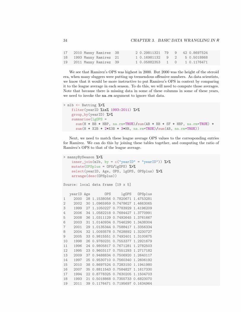
34 CHAPTER 3. BASIC DATA WRANGLING IN R
17 2010 Manny Ramirez 38 2 0.29811321 79 9 42 0.8697524
18 1993 Manny Ramirez 21 1 0.16981132 9 2 5 0.5018868
19 2011 Manny Ramirez 39 1 0.05882353 1 0 1 0.1176471
We see that Ramirez’s OPS was highest in 2000. But 2000 was the height of the steroidera, when many sluggers were putting up tremendous offensive numbers. As data scientists,we know that it would be more instructive to put Ramirez’s OPS in context by comparingit to the league average in each season. To do this, we will need to compute those averages.Note that because there is missing data in some of these columns in some of these years,we need to invoke the na.rm argument to ignore that data.
> mlb <- Batting %>%
filter(yearID %in% 1993:2011) %>%
group_by(yearID) %>%
summarise(lgOPS =
sum(H + BB + HBP, na.rm=TRUE)/sum(AB + BB + SF + HBP, na.rm=TRUE) +
sum(H + X2B + 2*X3B + 3*HR, na.rm=TRUE)/sum(AB, na.rm=TRUE))
Next, we need to match these league average OPS values to the corresponding entriesfor Ramirez. We can do this by joining these tables together, and computing the ratio ofRamirez’s OPS to that of the league average.
> mannyBySeason %>%
inner_join(mlb, by = c("yearID" = "yearID")) %>%
mutate(OPSplus = OPS/lgOPS) %>%
select(yearID, Age, OPS, lgOPS, OPSplus) %>%
arrange(desc(OPSplus))
Source: local data frame [19 x 5]
yearID Age OPS lgOPS OPSplus
1 2000 28 1.1538056 0.7820671 1.4753281
2 2002 30 1.0965959 0.7478627 1.4663065
3 1999 27 1.1050227 0.7783929 1.4196209
4 2006 34 1.0582218 0.7684427 1.3770991
5 2008 36 1.0311129 0.7492645 1.3761667
6 2003 31 1.0140934 0.7546290 1.3438304
7 2001 29 1.0135344 0.7588417 1.3356334
8 2004 32 1.0093578 0.7628892 1.3230727
9 2005 33 0.9815551 0.7492401 1.3100675
10 1998 26 0.9760231 0.7553377 1.2921679
11 1996 24 0.9805817 0.7671281 1.2782503
12 1995 23 0.9603117 0.7551293 1.2717182
13 2009 37 0.9488834 0.7506920 1.2640117
14 1997 25 0.9530710 0.7560340 1.2606192
15 2010 38 0.8697524 0.7283150 1.1941980
16 2007 35 0.8811543 0.7584827 1.1617330
17 1994 22 0.8778325 0.7630205 1.1504703
18 1993 21 0.5018868 0.7355733 0.6823070
19 2011 39 0.1176471 0.7195697 0.1634964
3.4. EXTENDED EXAMPLE: MANNY RAMIREZ 35
In this case, 2000 still ranks as Ramirez’s best season relative to his peers, but noticethat his 1999 season has fallen from 2nd to 3rd. His own steroid use notwithstanding,Ramirez posted 17 consecutive seasons with an OPS that was at least 15% better than theaverage across the major leagues – a truly impressive feat.
Finally, not all joins are the same. An inner join requires corresponding entries in bothtables. Conversely, a left join returns result for as many rows as there are in the firsttable, regardless of whether there are matches in the second table. Thus, an inner join isbidirectional, whereas in a left join, the order in which you specify the tables matters.
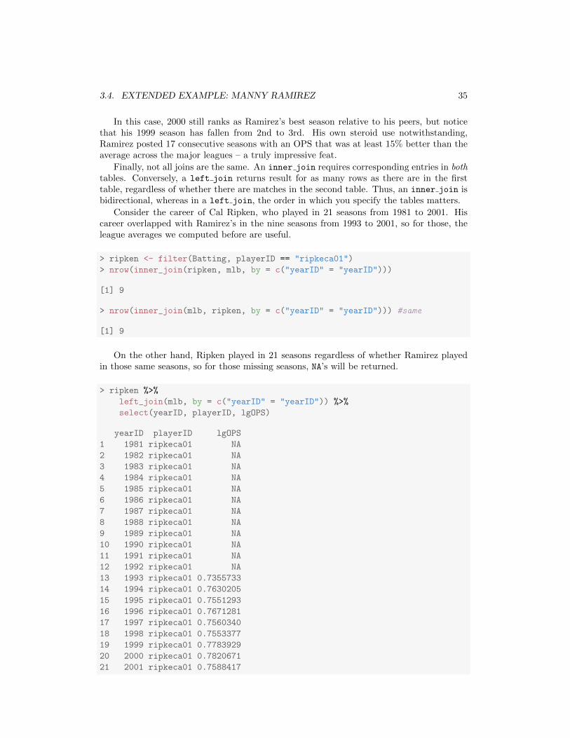
Consider the career of Cal Ripken, who played in 21 seasons from 1981 to 2001. Hiscareer overlapped with Ramirez’s in the nine seasons from 1993 to 2001, so for those, theleague averages we computed before are useful.
> ripken <- filter(Batting, playerID == "ripkeca01")
> nrow(inner_join(ripken, mlb, by = c("yearID" = "yearID")))
[1] 9
> nrow(inner_join(mlb, ripken, by = c("yearID" = "yearID"))) #same
[1] 9
On the other hand, Ripken played in 21 seasons regardless of whether Ramirez playedin those same seasons, so for those missing seasons, NA’s will be returned.
> ripken %>%
left_join(mlb, by = c("yearID" = "yearID")) %>%
select(yearID, playerID, lgOPS)
yearID playerID lgOPS
1 1981 ripkeca01 NA
2 1982 ripkeca01 NA
3 1983 ripkeca01 NA
4 1984 ripkeca01 NA
5 1985 ripkeca01 NA
6 1986 ripkeca01 NA
7 1987 ripkeca01 NA
8 1988 ripkeca01 NA
9 1989 ripkeca01 NA
10 1990 ripkeca01 NA
11 1991 ripkeca01 NA
12 1992 ripkeca01 NA
13 1993 ripkeca01 0.7355733
14 1994 ripkeca01 0.7630205
15 1995 ripkeca01 0.7551293
16 1996 ripkeca01 0.7671281
17 1997 ripkeca01 0.7560340
18 1998 ripkeca01 0.7553377
19 1999 ripkeca01 0.7783929
20 2000 ripkeca01 0.7820671
21 2001 ripkeca01 0.7588417
36 CHAPTER 3. BASIC DATA WRANGLING IN R
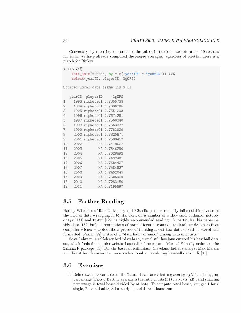
Conversely, by reversing the order of the tables in the join, we return the 19 seasonsfor which we have already computed the league averages, regardless of whether there is amatch for Ripken.
> mlb %>%
left_join(ripken, by = c("yearID" = "yearID")) %>%
select(yearID, playerID, lgOPS)
Source: local data frame [19 x 3]
yearID playerID lgOPS
1 1993 ripkeca01 0.7355733
2 1994 ripkeca01 0.7630205
3 1995 ripkeca01 0.7551293
4 1996 ripkeca01 0.7671281
5 1997 ripkeca01 0.7560340
6 1998 ripkeca01 0.7553377
7 1999 ripkeca01 0.7783929
8 2000 ripkeca01 0.7820671
9 2001 ripkeca01 0.7588417
10 2002 NA 0.7478627
11 2003 NA 0.7546290
12 2004 NA 0.7628892
13 2005 NA 0.7492401
14 2006 NA 0.7684427
15 2007 NA 0.7584827
16 2008 NA 0.7492645
17 2009 NA 0.7506920
18 2010 NA 0.7283150
19 2011 NA 0.7195697
3.5 Further Reading
Hadley Wickham of Rice University and RStudio is an enormously influential innovator inthe field of data wrangling in R. His work on a number of widely-used packages, notablydplyr [131] and tidyr [129] is highly recommended reading. In particular, his paper ontidy data [132] builds upon notions of normal forms – common to database designers fromcomputer science – to describe a process of thinking about how data should be stored andformatted. Finzer [28] writes of a “data habit of mind” among data scientists.
Sean Lahman, a self-described “database journalist”, has long curated his baseball dataset, which feeds the popular website baseball-reference.com. Michael Friendly maintains theLahman R package [33]. For the baseball enthusiast, Cleveland Indians analyst Max Marchiand Jim Albert have written an excellent book on analyzing baseball data in R [81].
3.6 Exercises
1. Define two new variables in the Teams data frame: batting average (BA) and sluggingpercentage (SLG). Batting average is the ratio of hits (H) to at-bats (AB), and sluggingpercentage is total bases divided by at-bats. To compute total bases, you get 1 for asingle, 2 for a double, 3 for a triple, and 4 for a home run.
3.6. EXERCISES 37
> Teams <- mutate(Teams, BA = H/AB, SLG = (H + X2B + 2*X3B + 3*HR)/AB)
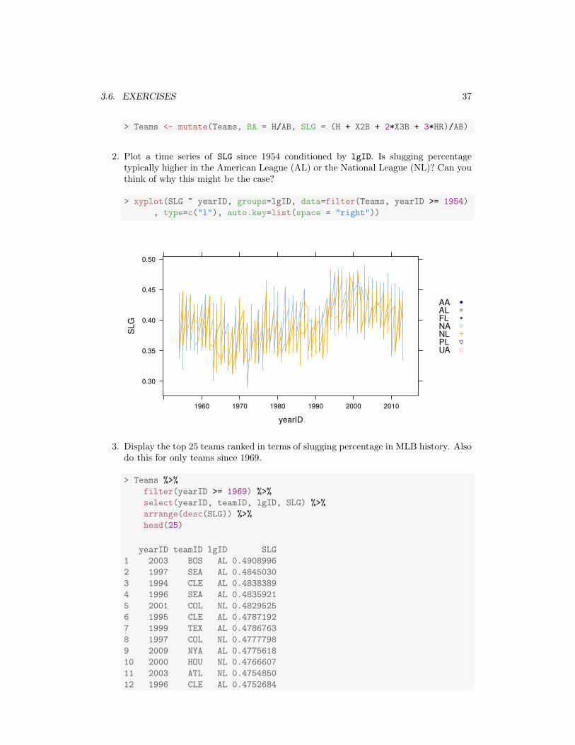
2. Plot a time series of SLG since 1954 conditioned by lgID. Is slugging percentagetypically higher in the American League (AL) or the National League (NL)? Can youthink of why this might be the case?
> xyplot(SLG ~ yearID, groups=lgID, data=filter(Teams, yearID >= 1954)
, type=c("l"), auto.key=list(space = "right"))
yearID
SLG
0.30
0.35
0.40
0.45
0.50
1960 1970 1980 1990 2000 2010
AAALFLNANLPLUA
●
3. Display the top 25 teams ranked in terms of slugging percentage in MLB history. Alsodo this for only teams since 1969.
> Teams %>%
filter(yearID >= 1969) %>%
select(yearID, teamID, lgID, SLG) %>%
arrange(desc(SLG)) %>%
head(25)
yearID teamID lgID SLG
1 2003 BOS AL 0.4908996
2 1997 SEA AL 0.4845030
3 1994 CLE AL 0.4838389
4 1996 SEA AL 0.4835921
5 2001 COL NL 0.4829525
6 1995 CLE AL 0.4787192
7 1999 TEX AL 0.4786763
8 1997 COL NL 0.4777798
9 2009 NYA AL 0.4775618
10 2000 HOU NL 0.4766607
11 2003 ATL NL 0.4754850
12 1996 CLE AL 0.4752684
38 CHAPTER 3. BASIC DATA WRANGLING IN R
13 2000 ANA AL 0.4724591
14 1996 COL NL 0.4724508
15 2004 BOS AL 0.4723776
16 2000 SFN NL 0.4720058
17 1996 BAL AL 0.4719634
18 1999 COL NL 0.4716585
19 1995 COL NL 0.4707649
20 2001 TEX AL 0.4707124
21 2000 CLE AL 0.4701742
22 2000 CHA AL 0.4700673
23 2000 TOR AL 0.4692619
24 1996 TEX AL 0.4686075
25 2005 TEX AL 0.4683345
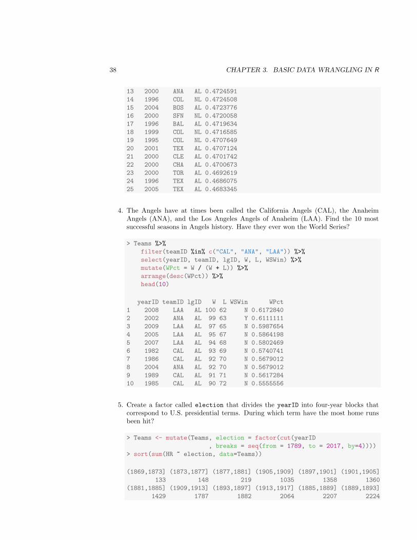
4. The Angels have at times been called the California Angels (CAL), the AnaheimAngels (ANA), and the Los Angeles Angels of Anaheim (LAA). Find the 10 mostsuccessful seasons in Angels history. Have they ever won the World Series?
> Teams %>%
filter(teamID %in% c("CAL", "ANA", "LAA")) %>%
select(yearID, teamID, lgID, W, L, WSWin) %>%
mutate(WPct = W / (W + L)) %>%
arrange(desc(WPct)) %>%
head(10)
yearID teamID lgID W L WSWin WPct
1 2008 LAA AL 100 62 N 0.6172840
2 2002 ANA AL 99 63 Y 0.6111111
3 2009 LAA AL 97 65 N 0.5987654
4 2005 LAA AL 95 67 N 0.5864198
5 2007 LAA AL 94 68 N 0.5802469
6 1982 CAL AL 93 69 N 0.5740741
7 1986 CAL AL 92 70 N 0.5679012
8 2004 ANA AL 92 70 N 0.5679012
9 1989 CAL AL 91 71 N 0.5617284
10 1985 CAL AL 90 72 N 0.5555556
5. Create a factor called election that divides the yearID into four-year blocks thatcorrespond to U.S. presidential terms. During which term have the most home runsbeen hit?
> Teams <- mutate(Teams, election = factor(cut(yearID
, breaks = seq(from = 1789, to = 2017, by=4))))
> sort(sum(HR ~ election, data=Teams))
(1869,1873] (1873,1877] (1877,1881] (1905,1909] (1897,1901] (1901,1905]
133 148 219 1035 1358 1360
(1881,1885] (1909,1913] (1893,1897] (1913,1917] (1885,1889] (1889,1893]
1429 1787 1882 2064 2207 2224
3.6. EXERCISES 39
(1917,1921] (1941,1945] (1921,1925] (1925,1929] (1929,1933] (1933,1937]
2249 4017 4100 4227 5059 5463
(1937,1941] (1945,1949] (1949,1953] (1953,1957] (1957,1961] (1965,1969]
5822 6039 7713 8657 9348 10156
(1961,1965] (1973,1977] (1977,1981] (1969,1973] (1981,1985] (1989,1993]
11155 11226 11257 11928 13540 13768
(1985,1989] (1993,1997] (2009,2013] (2005,2009] (2001,2005] (1997,2001]
14534 16989 18760 20263 20734 21743
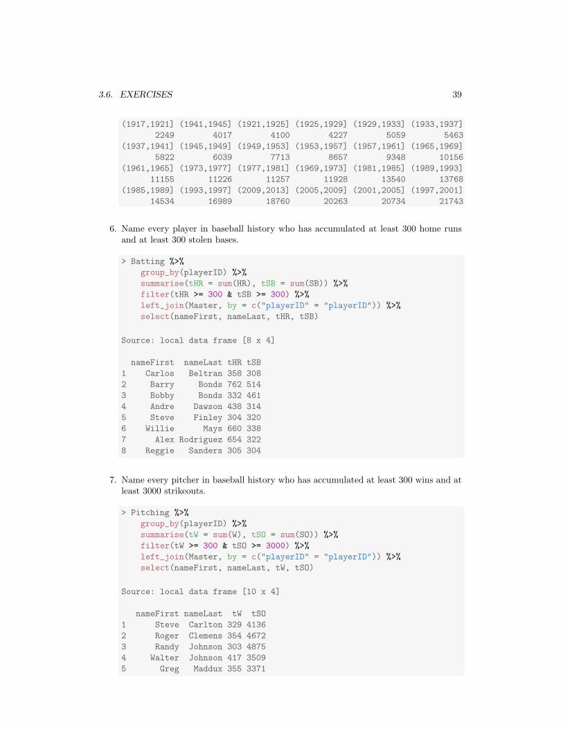
6. Name every player in baseball history who has accumulated at least 300 home runsand at least 300 stolen bases.
> Batting %>%
group_by(playerID) %>%
summarise(tHR = sum(HR), tSB = sum(SB)) %>%
filter(tHR >= 300 & tSB >= 300) %>%
left_join(Master, by = c("playerID" = "playerID")) %>%
select(nameFirst, nameLast, tHR, tSB)
Source: local data frame [8 x 4]
nameFirst nameLast tHR tSB
1 Carlos Beltran 358 308
2 Barry Bonds 762 514
3 Bobby Bonds 332 461
4 Andre Dawson 438 314
5 Steve Finley 304 320
6 Willie Mays 660 338
7 Alex Rodriguez 654 322
8 Reggie Sanders 305 304
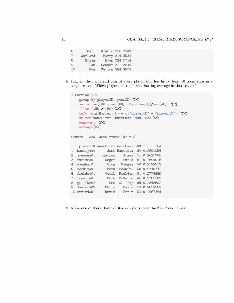
7. Name every pitcher in baseball history who has accumulated at least 300 wins and atleast 3000 strikeouts.
> Pitching %>%
group_by(playerID) %>%
summarise(tW = sum(W), tSO = sum(SO)) %>%
filter(tW >= 300 & tSO >= 3000) %>%
left_join(Master, by = c("playerID" = "playerID")) %>%
select(nameFirst, nameLast, tW, tSO)
Source: local data frame [10 x 4]
nameFirst nameLast tW tSO
1 Steve Carlton 329 4136
2 Roger Clemens 354 4672
3 Randy Johnson 303 4875
4 Walter Johnson 417 3509
5 Greg Maddux 355 3371
40 CHAPTER 3. BASIC DATA WRANGLING IN R
6 Phil Niekro 318 3342
7 Gaylord Perry 314 3534
8 Nolan Ryan 324 5714
9 Tom Seaver 311 3640
10 Don Sutton 324 3574
8. Identify the name and year of every player who has hit at least 50 home runs in asingle season. Which player had the lowest batting average in that season?
> Batting %>%
group_by(playerID, yearID) %>%
summarise(tHR = sum(HR), BA = sum(H)/sum(AB)) %>%
filter(tHR >= 50) %>%
left_join(Master, by = c("playerID" = "playerID")) %>%
select(nameFirst, nameLast, tHR, BA) %>%
ungroup() %>%
arrange(BA)
Source: local data frame [43 x 5]
playerID nameFirst nameLast tHR BA
1 bautijo02 Jose Bautista 54 0.2601054
2 jonesan01 Andruw Jones 51 0.2627986
3 marisro01 Roger Maris 61 0.2694915
4 vaughgr01 Greg Vaughn 50 0.2722513
5 mcgwima01 Mark McGwire 58 0.2740741
6 fieldce01 Cecil Fielder 51 0.2774869
7 mcgwima01 Mark McGwire 65 0.2783109
8 griffke02 Ken Griffey 56 0.2843602
9 davisch02 Chris Davis 53 0.2859589
10 ortizda01 David Ortiz 54 0.2867384
.. ... ... ... ... ...
9. Make one of these Baseball Records plots from the New York Times.