basic econometrics - faculty of business and economics ... econometrics.pdf · executive mba...

Executive MBA 2007-2008

emba bridge- 2006/2007 1

Basic EconometricsBasic Econometrics

Christopher Christopher GrigoriouGrigoriou

ExecutiveExecutive MBAMBA--HEC LausanneHEC Lausanne

2007/20082007/2008



OverviewOverview

Objectives of the dayObjectives of the day•• Interpreting Econometric ApplicationsInterpreting Econometric Applications

••Understanding how it worksUnderstanding how it works

Program of the dayProgram of the day••Introduction (why? how? basic concepts)Introduction (why? how? basic concepts)

••InterpretationsInterpretations

••CaseCase--studystudy

ExecutiveExecutive MBA MBA –– HEC Lausanne 2007/2008HEC Lausanne 2007/2008



1.1. Introduction to EconometricsIntroduction to Econometrics

=> What for ?=> What for ?

�� Impact AnalysisImpact Analysis

�� To evaluate the success/failure of a To evaluate the success/failure of a

project, reform, law,project, reform, law,……

�� To test any economic theoryTo test any economic theory




1.1. Introduction to EconometricsIntroduction to Econometrics

=> How ?=> How ?

•• Apply statistical methods to economic Apply statistical methods to economic

datadata

•• Econometric approach: Econometric approach:

-- Develop working model from an Develop working model from an

economic theoryeconomic theory

-- Estimate model with real world data.Estimate model with real world data.

Real world data is not perfectReal world data is not perfect




Some examplesSome examples

•• Keynesian Consumption FunctionKeynesian Consumption Function

•• Price and QuantityPrice and Quantity

•• Philips CurvePhilips Curve

•• Production FunctionProduction Function




Keynesian Consumption FunctionKeynesian Consumption Function

•• Theory: people increase consumption as Theory: people increase consumption as income increases, but not by as much as the income increases, but not by as much as the increase in their income.increase in their income.

–– Marginal Propensity to Consume (MPC) is the Marginal Propensity to Consume (MPC) is the change in consumption divided by change in change in consumption divided by change in income.income.




�� C = C = αα + + β.β.II–– C = ConsumptionC = Consumption

−− αα = Intercept= Intercept

–– I = IncomeI = Income

−− ββ = slope (how much C changes for a given = slope (how much C changes for a given

change in I)change in I)

�� Not an econometric modelNot an econometric model

–– Assumes a deterministic relationshipAssumes a deterministic relationship

Keynesian Consumption FunctionKeynesian Consumption Function




�� C = C = α + α + ββII + + εεε ε = error term= error term

�� Error term captures several factors:Error term captures several factors:

–– omitted variablesomitted variables

–– measurement error in the dependent variablemeasurement error in the dependent variable

–– randomness of human behaviorrandomness of human behavior

Keynesian Consumption Function Keynesian Consumption Function

=> Econometric Model=> Econometric Model

•• Expected Results: Expected Results: αα > 0 and 0 < > 0 and 0 < ββ < 1< 1

ββ represents the MPCrepresents the MPC




Ordinary Least SquaresOrdinary Least Squares

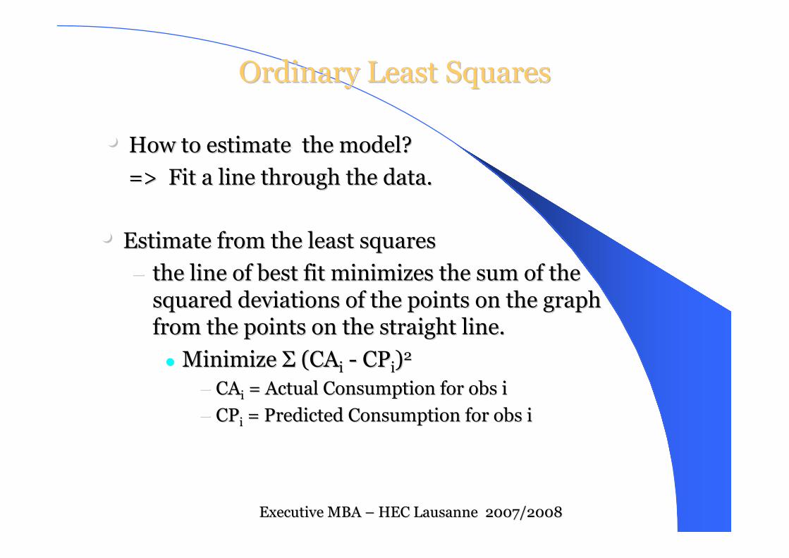
•• Estimate from the least squaresEstimate from the least squares

–– the line of best fit minimizes the sum of the the line of best fit minimizes the sum of the

squared deviations of the points on the graph squared deviations of the points on the graph

from the points on the straight line.from the points on the straight line.

�� Minimize Minimize ΣΣ ((CACAii -- CPCPii))22

–– CACAii = Actual Consumption for = Actual Consumption for obsobs ii

–– CPCPii = Predicted Consumption for = Predicted Consumption for obsobs ii

•• How to estimate the model? How to estimate the model?

=> Fit a line through the data.=> Fit a line through the data.




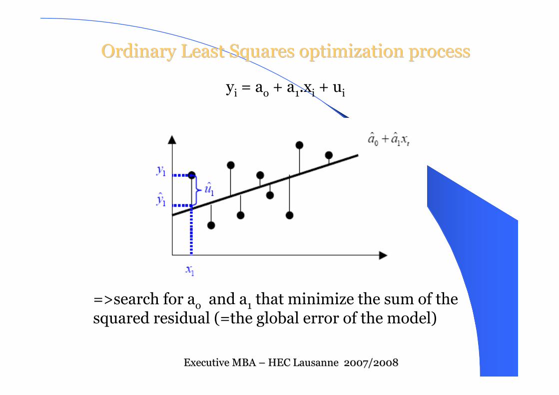
Ordinary Least Squares optimization processOrdinary Least Squares optimization process

=>search for ao and a1 that minimize the sum of the squared residual (=the global error of the model)

yi = ao + a1.xi + ui




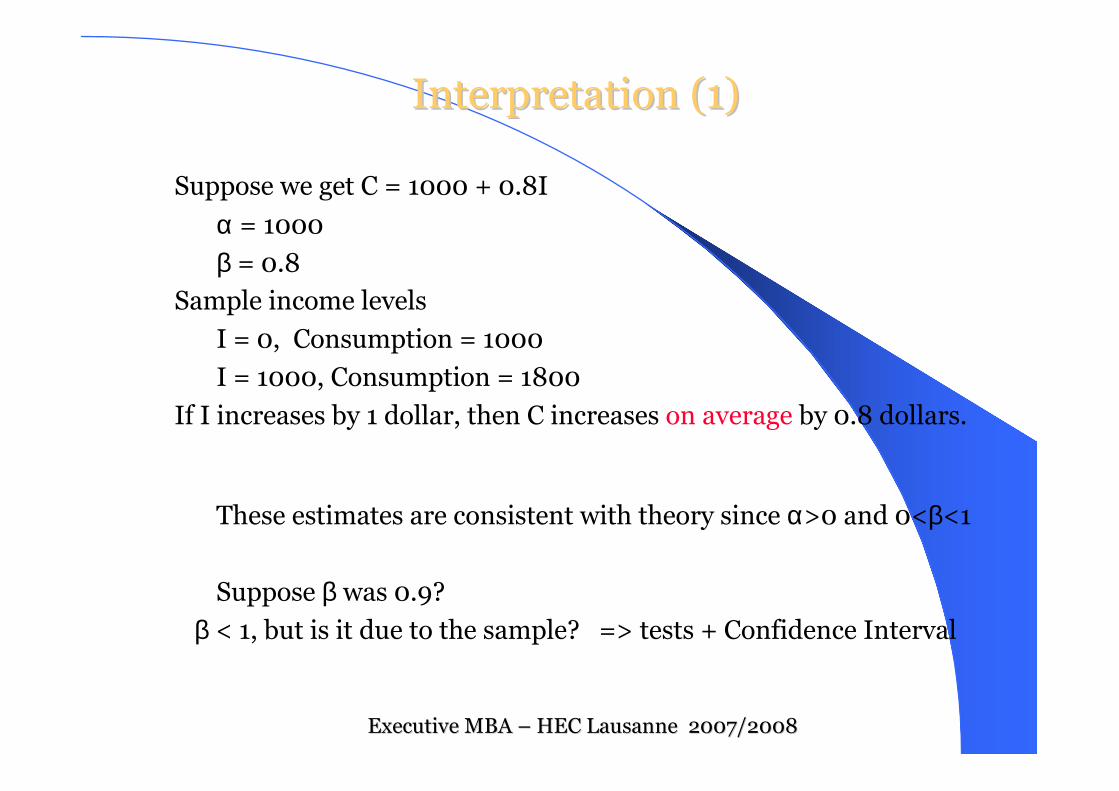
• Suppose we get C = 1000 + 0.8I

α = 1000β = 0.8

• Sample income levels

– I = 0, Consumption = 1000

– I = 1000, Consumption = 1800

• If I increases by 1 dollar, then C increases on average by 0.8 dollars.

Interpretation (1)Interpretation (1)

– These estimates are consistent with theory since α>0 and 0<β<1

– Suppose β was 0.9? β < 1, but is it due to the sample? => tests + Confidence Interval




Interpretation (2)Interpretation (2)

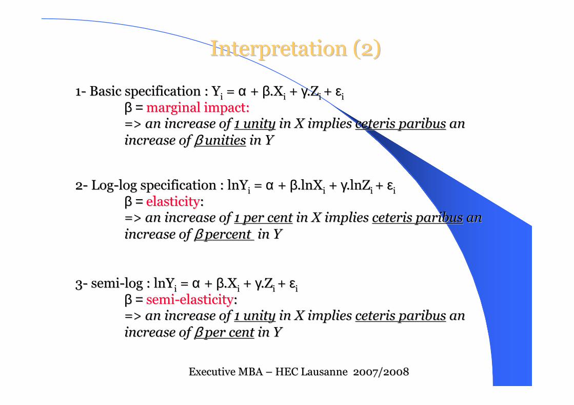
11-- Basic specification : Basic specification : YYii = = αα + + ββ..XXii ++ γγ..ZZii + + εεiiβ = β = marginal impact:marginal impact:=> => an an increaseincrease ofof 1 1 unityunity in X in X impliesimplies ceterisceteris paribusparibus an an

increaseincrease ofof β β unitiesunities in Yin Y

22-- LogLog--log specification : log specification : lnlnYYii = = αα + + ββ..lnXlnXii ++ γγ..lnZlnZii + + εεiiβ = β = elasticityelasticity::=> => an an increaseincrease ofof 1 1 perper centcent in X in X impliesimplies ceterisceteris paribusparibus an an

increaseincrease ofof β β percent percent in Yin Y

33-- semisemi--log : log : lnlnYYii = = αα + + ββ..XXii ++ γγ..ZZii + + εεiiβ = β = semisemi--elasticityelasticity::=> => an an increaseincrease ofof 1 1 unityunity in X in X impliesimplies ceterisceteris paribusparibus an an

increaseincrease ofof β β perper centcent in Yin Y




Other examples (1)Other examples (1)

�� Price and QuantityPrice and Quantity

�� Demand and Demand and elasticitieselasticitiesof demandof demand

�� lnln Q = Q = α + βα + β lnPlnP + + εε

�� Phillips CurvePhillips Curve

–– Relationship between change in money wages and Relationship between change in money wages and unemploymentunemployment

�� ∆∆ww = f (= f (∆∆u)u)




�� Production FunctionProduction Function

–– Relationship between inputs and outputs. Relationship between inputs and outputs.

�� Y = f (K,L) Y = f (K,L)

�� Cobb Douglas Y = Cobb Douglas Y = AKAK aaLLββ

�� Wage equationWage equation

lnln W = W = αα00+ + αα11EDUC + EDUC + αα22EXP + EXP + αα33GENDER + GENDER + αα44RACE + RACE + + + εεii

Other examples (2)Other examples (2)




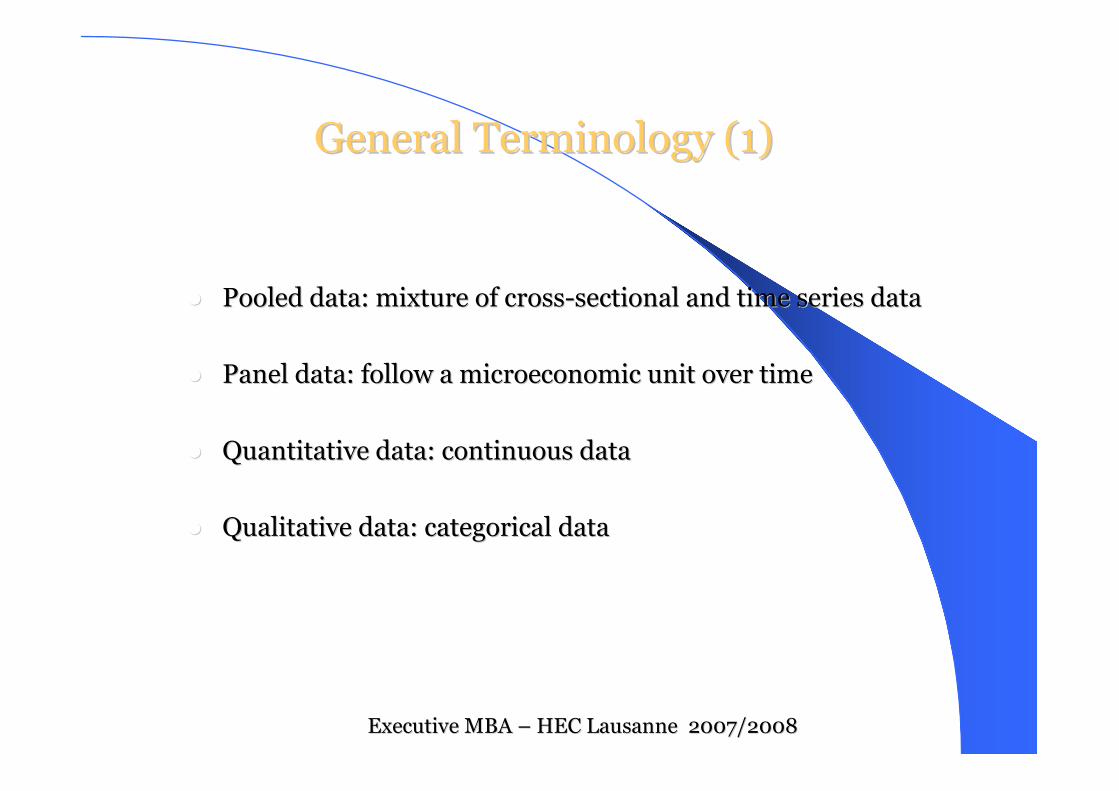
General Terminology (1)General Terminology (1)

�� Pooled data: mixture of crossPooled data: mixture of cross--sectional and time series datasectional and time series data

�� Panel data: follow a microeconomic unit over timePanel data: follow a microeconomic unit over time

�� Quantitative data: continuous dataQuantitative data: continuous data

�� Qualitative data: categorical dataQualitative data: categorical data




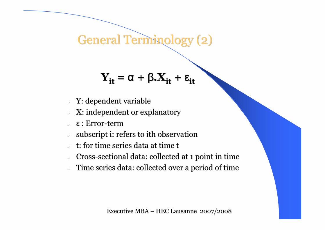
General Terminology (2)General Terminology (2)

YYiitt= = αααααααα + + ββββββββ..XX

iitt+ + εεεεεεεε

iitt

�� Y: dependent variableY: dependent variable

�� X: independent or explanatoryX: independent or explanatory

�� ε : ε : ErrorError--termterm

�� subscript i: refers to subscript i: refers to ithith observationobservation

�� t: for time series data at time tt: for time series data at time t

�� CrossCross--sectional data: collected at 1 point in timesectional data: collected at 1 point in time

�� Time series data: collected over a period of time Time series data: collected over a period of time




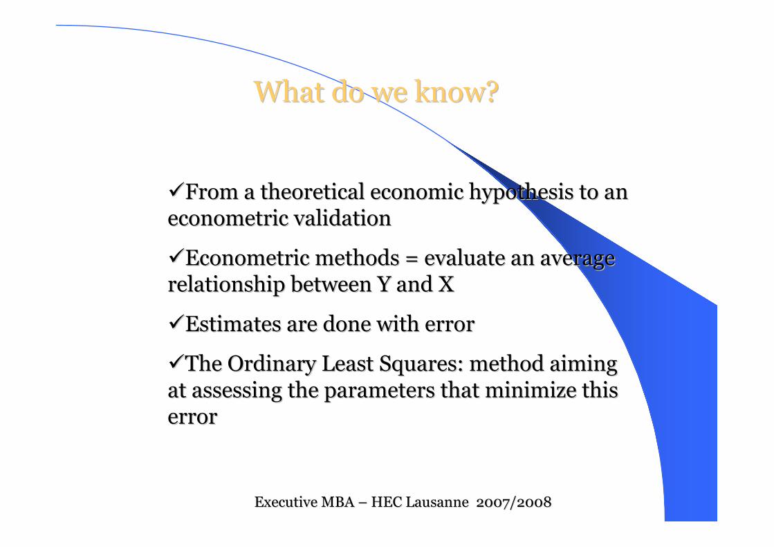
WhatWhat do do wewe know?know?

��FromFrom a a theoreticaltheoretical economiceconomic hypothesishypothesis to an to an

econometriceconometric validationvalidation

��EconometricEconometric methodsmethods = = evaluateevaluate an an averageaverage

relationshiprelationship betweenbetween Y and XY and X

��EstimatesEstimates are are donedone withwith errorerror

��The The OrdinaryOrdinary Least Squares: Least Squares: methodmethod aimingaiming

atat assessingassessing the the parametersparameters thatthat minimizeminimize thisthis

errorerror




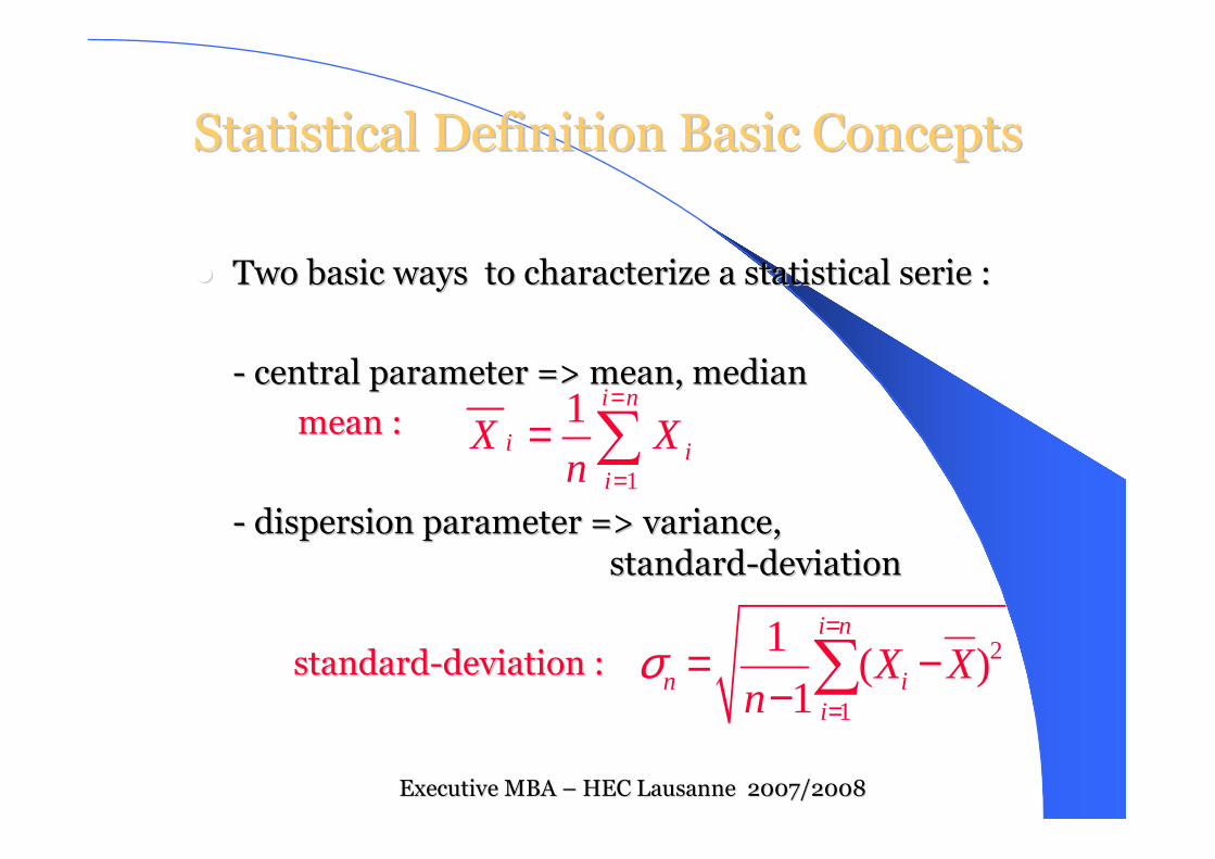
StatisticalStatistical DefinitionDefinition Basic ConceptsBasic Concepts

�� TwoTwo basic basic waysways to to characterizecharacterize a a statisticalstatistical serieserie : :

-- central central parameterparameter => => meanmean, , medianmedian

meanmean ::

-- dispersion dispersion parameterparameter => variance, => variance,

standardstandard--deviationdeviation

standardstandard--deviationdeviation ::

1

1 i n

i ii

X Xn

=

=

= ∑

2

1

1( )

1

i n

n ii

X Xn

σ=

=

= −− ∑




ExampleExample: 2 : 2 differentdifferent classroomsclassrooms

Exam Exam ofof StatisticsStatistics……

�� 2 groups 2 groups withwith on on averageaverage exactlyexactly thethe samesame markmark…… => 11.5=> 11.5

�� WhatWhat information information doesdoes itit provideprovide on on youryour ownown resultresult??




Class AClass A

5.9σ11.5Mean

34.3Var.149.5Sum

72.258.511.52013

49711.518.512

30.255.511.51711

20.254.511.51610

12.253.511.5159

6.252.511.5148

0.250.511.5127

2.25-1.511.5106

6.25-2.511.595

20.25-4.511.574

30.25-5.511.563

72.25-8.511.532

90.25-9.511.521

(Xi-mean)²Xi-MeanMeanXiRank




Class BClass B

1.04σ11.5Mean

1.08Var.149.5Sum

2.251.511.51313

2.251.511.51312

1111.512.511

1111.512.510

0.250.511.5129

0011.511.58

0011.511.57

0.25-0.511.5116

0.25-0.511.5115

0.25-0.511.5114

1-111.510.53

2.25-1.511.5102

2.25-1.511.5101

(Xi-mean)²Xi-MeanMeanXiRank




=> To => To characterizecharacterize a a serieserie youyou needneed�� TheThe meanmean ofof thethe serieserie (central (central parameterparameter))

�� TheThe standardstandard--deviationdeviation (dispersion)(dispersion)

=>=>……ofof course, course, thethe answeranswer alsoalso

dependsdepends on on thethe dispersion (dispersion (standardstandard--

deviationdeviation))




�� SameSame thingthing withwith a coefficient a coefficient estimateestimate……

=> => thethe coefficient coefficient isis an an averagedaveraged impactimpact

=> => itsits significancesignificance dependsdepends on on itsits dispersiondispersion, , i.e. i.e. thethe accuracyaccuracy associatedassociated to to thethe estimateestimate

DonDon’’tt forgetforget! ! thethe predictionspredictions are are donedone withwith errorerror!!

Y = Y = αα + + ββXX + + εε

⇒⇒Given the error in the estimate or the inaccuracy in the Given the error in the estimate or the inaccuracy in the

estimate (assessed by the dispersion)estimate (assessed by the dispersion)

⇒⇒ is is ββ significantly different fromsignificantly different from zero?zero?




Estimation Estimation ofof thethe educationeducation return (1)return (1)

•• OneOne ((perhapsperhaps youyou?) ?) wantswants to to knowknow thethe impact impact ofof anan

additionnaladditionnal yearyear ofof educationeducation on on hishis wagewage

•• EconomicEconomic TheoryTheory : Mincer: Mincer’’s s EquationEquation

•• EconometricEconometric point: point: howhow bigbig isis ββ ??=> => lwagelwage

ii= = αα + + ββ..educeduc

ii++ γγ..experexper

ii++ δδ. . expersqexpersq

ii++ εε

ii




=> 428 observations in => 428 observations in thethe samplesample

=>=>RR--squaredsquared = 15.68%= 15.68%

Our Our modelmodel predictspredicts 15.68% 15.68% ofof thethe fluctuations fluctuations ofof thethe wageswages




lwage

educβ ∂=

∂

•• ((averageaverage) coefficient ) coefficient

=> 0.1075=> 0.1075

=> => AnyAny additionaladditional yearyear ofof educationeducation impliesimplies on on

averageaverage an an increaseincrease ofof 0.1075% in 0.1075% in thethe wagewage

•• NotNot onlyonly a a meanmean (coefficient), but (coefficient), but alsoalso a a standard standard

deviationdeviation (0.0141465)(0.0141465)……as as anyany otherother statisticalstatistical serieserie

•• TheThe standard standard deviationdeviation providesprovides information on information on thethe

accuracyaccuracy ofof thethe estimateestimate..




� Coefficient estimated with error

� standard deviation

⇒ Confidence Interval :

⇒ 95% chances for the coefficient to be in the interval

( β β −− 2 σ = 0.07968 ; β + 2 σ = 0.1352956) 2 σ = 0.07968 ; β + 2 σ = 0.1352956)




�� IsIs β β significantlysignificantly differentdifferent fromfrom zerozero? ?

�� A test A test classicallyclassically usedused to compare to compare averagesaverages: t: t--test.test.

=>Compare the actual coeff.( ) with the restricted coeff.( ) weighted by the dispersion (= a measure of theaccuracy of the estimate)

ˆ

ˆt β

β

β βσ−=

β̂σ β

β̂� = 0.1075; = 0 !! = 0.01414 => 0.1075

7.600.01414

tβ = =

β̂

β

�� SoSo whatwhat? ?

β̂σ




�� HH00: : ββ = 0= 0

�� ComputeCompute a a tt--statisticstatistic

�� || tt--statisticstatistic || > 2 => > 2 => rejectreject HH00

=> β => β significantlysignificantly differentdifferent fromfrom zerozero ((whatwhat wewe expectedexpected!!)!!)

�� || tt--statisticstatistic || < 2 => < 2 => cannotcannot rejectreject HH00

=> β ΝΟΤ => β ΝΟΤ significantlysignificantly differentdifferent fromfrom zerozero ((nono impact impact ofof

studyingstudying oneone more more yearyear on on mymy wageswages !!)!!)




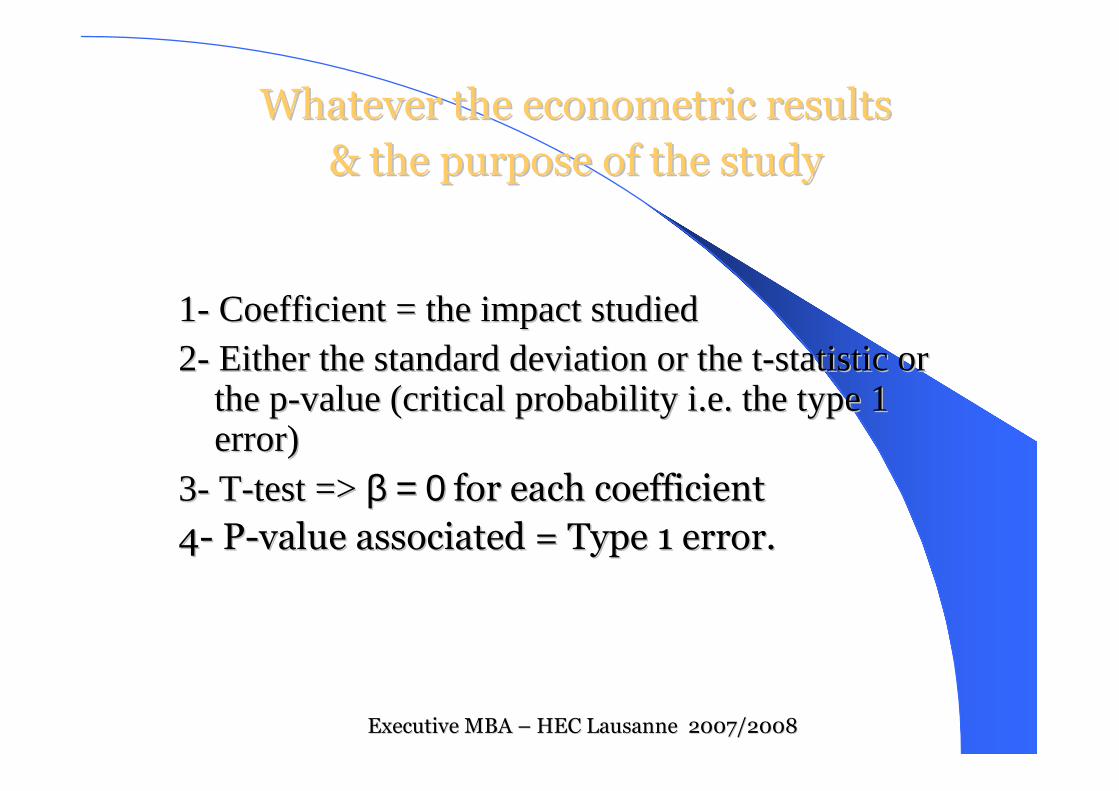
11-- Coefficient = Coefficient = thethe impact impact studiedstudied22-- EitherEither thethestandard standard deviationdeviationor or thethett--statisticstatisticor or

thethepp--value (value (criticalcritical probabilityprobability i.e. i.e. thethetype 1 type 1 errorerror) )

33-- TT--test => test => β = 0 β = 0 for for eacheach coefficientcoefficient

44-- PP--value value associatedassociated = Type 1 = Type 1 errorerror..

WhateverWhatever thethe econometriceconometric resultsresults

& & thethe purposepurpose ofof thethe studystudy




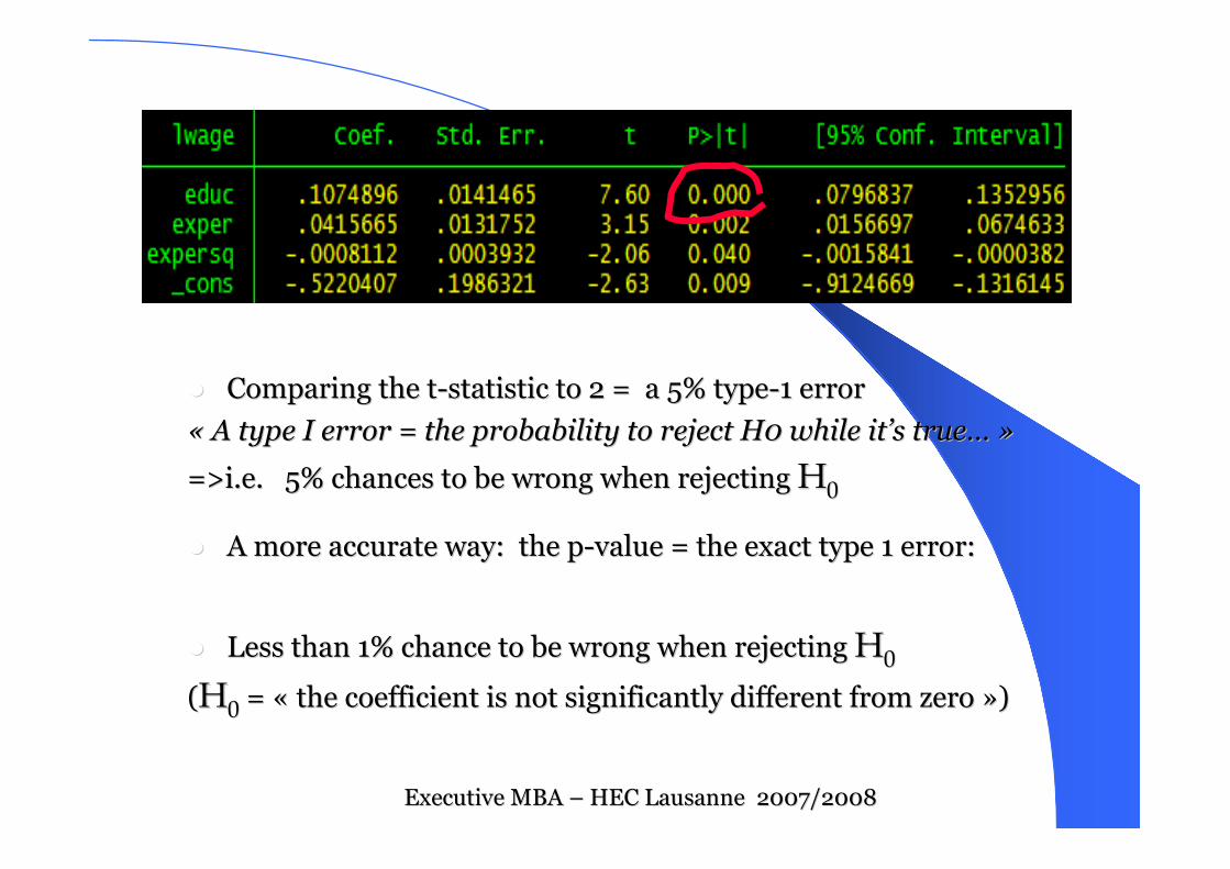
�� ComparingComparing thethe tt--statisticstatistic to 2 = a 5% typeto 2 = a 5% type--1 1 errorerror

«« A type I A type I errorerror = = thethe probabilityprobability to to rejectreject H0 H0 whilewhile itit’’s s truetrue…… »»

=>i.e. 5% chances to =>i.e. 5% chances to bebe wrongwrong whenwhen rejectingrejectingHH00

�� A more A more accurateaccurate wayway: : thethe pp--value = value = thethe exact type 1 exact type 1 errorerror::

�� LessLess thanthan 1% chance to 1% chance to bebe wrongwrong whenwhen rejectingrejectingHH00

((HH00= = «« thethe coefficient coefficient isis notnot significantlysignificantly differentdifferent fromfrom zerozero »»))




CaseCase--StudyStudy: : FeldsteinFeldstein andand HoriokaHorioka (1980)(1980)

�� FromFrom thethe liberalisationliberalisation ofof thethe capital capital flightsflights

=> => howhow diddid thethe capital capital reallyreally movemove ??

�� FeldsteinFeldstein andand HoriokaHorioka (1980) : (1980) : correlationcorrelation betweenbetweensavingssavings andand investmentsinvestments

�� TheThe impact impact ofof economiceconomic policypolicy dependsdepends on on thethe degreedegree

ofof mobilitymobility ofof thethe capitalcapital




Correlation between Savings and Investment

and the openness of the economy

1- Correlation between Savings and Investments close to 1:

⇒ Closed economyany increase in national savings induces an identical increase in investments=> low degree of capital mobility

2- Correlation between Savings and Investments close to 0:

⇒ Openned (integrated) economy: National savings respond to investment opportunities on the world market/ national investment is financed by savings from the rest of the world => highdegree of capital mobility




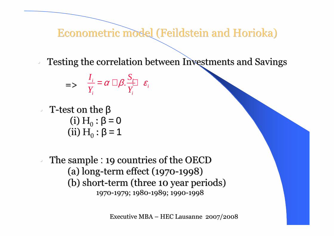
EconometricEconometric modelmodel ((FeildsteinFeildstein andand HoriokaHorioka))

.i ii

i i

I S

Y Yα β ε= + +

•• TestingTesting thethe correlationcorrelation betweenbetween InvestmentsInvestments andand SavingsSavings

=>=>

•• TT--test on test on thethe β β (i) (i) HH

00: : β = 0β = 0

((iiii) ) HH00: : β = 1β = 1

•• TheThe samplesample : : 19 countries 19 countries ofof thethe OECDOECD

(a) (a) longlong--termterm effecteffect (1970(1970--1998)1998)

(b) (b) shortshort--termterm ((threethree 10 10 yearyear periodsperiods))19701970--1979; 19801979; 1980--1989; 19901989; 1990--19981998




SavingSaving andand InvestmentInvestment: long : long periodperiod (1970(1970--98)98)

0.580.58RR-- SquaredSquared

1919ObservationsObservations

0.030.03((standardstandard--errorerror))

0.080.08ConstantConstant


0.620.62ssii

SavingSaving andand InvestmentInvestment: :

19701970--1998199811-- IsIs b b significantlysignificantly differentdifferent fromfromzerozero? ? HH

00: : β = 0β = 0

⇒⇒tt--test (to compare test (to compare meansmeans))

⇒⇒|| 4.85 4.85 || > 2> 2⇒⇒AtAt thethe 5% 5% levellevel HH

00isis rejectedrejected

⇒⇒Note Note thethe pp--value (value (computedcomputed by by thethe

software) software) isis inferiorinferior to 1%to 1%

⇒⇒In In thethe longlong--termterm wewe cannotcannot

concludeconclude to a to a perfectperfect degreedegree

ofof capital capital mobilitymobility

ˆ

ˆ 0.62 04.85

0.13tβ

β

β βσ− −= = =




SavingSaving andand InvestmentInvestment: long : long periodperiod (1970(1970--98)98)

0.580.58RR-- SquaredSquared



0.080.08ConstantConstant


0.620.62ssii

SavingSaving andand InvestmentInvestment: :

19701970--19981998 11-- IsIs ββ significantlysignificantly differentdifferent fromfromoneone? ? HH

00: : β = 1β = 1

⇒⇒tt--test (to compare test (to compare meansmeans))

⇒⇒|| 2.94 2.94 || > 2> 2⇒⇒AtAt thethe 5% 5% levellevel HH

00isis rejectedrejected

⇒⇒Note Note thethe pp--value (value (computedcomputed by by thethe

software) software) isis inferiorinferior to 1%to 1%

⇒⇒In In thethe longlong--termterm wewe cannotcannot

concludeconclude to to closedclosed economieseconomies

ˆ

ˆ 0.62 12.94

0.13tβ

β

β βσ− −= = =




SavingSaving andand InvestmentInvestment: : shortshort--termtermThreeThree 10 10 yearyear periodsperiods 19701970--79; 198079; 1980--89; 199089; 1990--9898

0.400.650.820.82ssii

0.150.140.140.14((standardstandard--errorerror))

0.110.080.080.08ConstantConstant

0.030.030.030.03((standardstandard--errorerror))

0.300.550.610.61RR-- SquaredSquared


(3)

1990-1998

(2)

1980-1989

(1)

1970-1979

Periods

Saving and Investment

=> => WhatWhat cancan youyou saysay about about opennessopenness ofof OECD countries OECD countries

overover eacheach 10 10 yearyear periodsperiods??




ExerciseExercise::


⇒⇒WhatWhat cancan youyou saysay about about opennessopenness ofof OECD countriesOECD countries

for for eacheach ofof thethe threethree periodsperiods??(for (for eacheach periodperiod: : perfectperfect capital capital mobilitymobility? ? ClosedClosed economieseconomies? ? EtcEtc……))

⇒⇒WhatWhat wouldwould youyou saysay regardingregarding thethe evolutionevolution ofof thethe

capital capital mobilitymobility overover thethe wholewhole periodperiod??




ExerciseExercise::


⇒⇒ ResultsResults::

⇒⇒ Conclusion:Conclusion:




ExerciseExercise::


⇒⇒ ResultsResults::

PeriodPeriod 1 : 1 : (i) (i) HH00: : ββ=0 => t = 5.93 => |t|>2 => rejection =0 => t = 5.93 => |t|>2 => rejection ofof HH

00

((iiii) ) HH00: : ββ=1 => t = =1 => t = --1.32 => |t|<2 => 1.32 => |t|<2 => nonnon--rejectionrejection ofof HH

00

⇒⇒ Conclusion: Conclusion: -- None None ofof thethe threethree periodsperiods withwith a a perfectperfect capital capital mobilitymobility

-- EvenEven a a behaviourbehaviour ofof closedclosed economieseconomies overover thethe firstfirst periodperiod

=> => A change A change towardtoward opennessopenness overover thethe 2 2 lastlast periodsperiods??

ˆ 0.82β =

ˆ 0.65β =

ˆ 0.40β =PeriodPeriod 3:3: (i) (i) HH00: : ββ=0 => t =2.67 => |t|>2 => rejection =0 => t =2.67 => |t|>2 => rejection ofof HH

00

((iiii) ) HH00: : ββ=1 => t = =1 => t = --4.04 => |t|>2 => rejection 4.04 => |t|>2 => rejection ofof HH

00

PeriodPeriod 2:2: (i) (i) HH00: : ββ=0 => t = 4.62 => |t|>2 => rejection =0 => t = 4.62 => |t|>2 => rejection ofof HH

00

((iiii) ) HH00: : ββ=1 => t = =1 => t = --2.46 => |t|>2 => rejection 2.46 => |t|>2 => rejection ofof HH

00




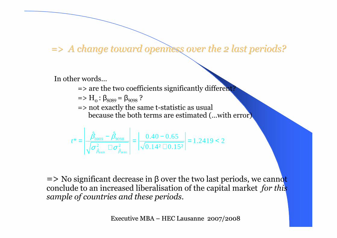
=> => A change A change towardtoward opennessopenness overover thethe 2 2 lastlast periodsperiods??

• In other words…=> are the two coefficients significantly different?

=> H0 : β8089

= β9098

?

=> not exactly the same t-statistic as usualbecause the both terms are estimated (…with error)

•

8089 9098

8089 9098

2 2ˆ ˆ

ˆ ˆ 0.40 0.65* 1.2419 2

0.14² 0.15²t

β β

β βσ σ

− −= = = <++

=> No significant decrease in β over the two last periods, we cannotconclude to an increased liberalisation of the capital market for thissample of countries and these periods.




ConclusionConclusion-- WhatWhat have have wewe learntlearnt??

� -

� -

� -

� -

� -

� -

� -




ConclusionConclusion-- WhatWhat have have wewe learntlearnt??

11-- Basic Basic methodologymethodology regardingregarding econometricseconometrics

-- EconomicEconomic problemproblem => data => => data => econometriceconometric validationvalidation

22-- CharacterizingCharacterizing a a statisticalstatistical serieserie

-- Central Central parameterparameter, dispersion , dispersion charactercharacter……

33-- TheThe mostmost commoncommon econometriceconometric estimatorestimator

-- OrdinaryOrdinary LeastLeast Squares, concept Squares, concept ofof errorerror--termterm

44-- Reading/Reading/interpretinginterpreting econometriceconometric resultsresults

-- RR--squaredsquared, Marginal impact, , Marginal impact, elasticityelasticity, , semisemi--elasticityelasticity, ,

confidence confidence intervalinterval, p, p--value,value,……

55-- StatisticalStatistical test test ofof thethe coefficientscoefficients

-- tt--test (test (studentstudent test): test): againstagainst a constant, a constant, againstagainst anotheranother estimateestimate


basic econometrics - faculty of business and economics ... econometrics.pdf · executive mba...

Documents