1

Interactions in Multiple Linear Regression

Basic Ideas

Interaction: An interaction occurs when an independent variable has a differenteffect on the outcome depending on the values of another independent variable.

Let’s look at some examples. Suppose that there is a cholesterol lowering drug that istested through a clinical trial. Suppose we are expecting a linear dose-response overa given range of drug dose, so that the picture looks like this:

This is a standard simple linear model. Now, however, suppose that we expect mento respond at an overall higher level compared to women. There are various waysthat this can happen. For example, if the difference in response between women andmen is constant throughout the range, we would expect a graph like this:

2

However, if men, have a steeper dose-response curve compared to women, we wouldexpect a picture like this:

3

On the other hand, if men, have a less steep dose-response curve compared to women,we would expect a picture like this:

Of these four graphs, the first indicates no difference between men and women, thesecond illustrates that there is a difference, but since it is constant, there is no inter-action term. The third and fourth graphs represent the situation with an interactionof the effect of the drug, depending on whether it is given to men or women.

In terms of regression equations, we have:

No effect of sex:

Y = α + β1 ∗ dose (+0× sex + 0× dose ∗ sex)

where Y represents the outcome (amount of cholesterol lowering), β1 representsthe effect of the drug (presumed here to be non-zero), and all other coefficientsfor the rest of the terms (effect of sex and interaction term) are zero.

Sex has an effect, but no interaction:

Y = α + β1 ∗ dose + β2 × sex (+0× dose ∗ sex)

Sex has an effect with an interaction:

Y = α + β1 ∗ dose + β2 × sex + β3 × dose ∗ sex

4

Let’s consider how to report the effects of sex and dose in the presence of interactionterms. If we consider the first of the above models, without any effect of sex, it istrivial to report. There is no effect of sex, and the coefficient β1 provides the effect ofdose. In particular, β1 represents the amount by which cholesterol changes for eachunit change in dose of the drug.

If we consider the second model, where there are effects of both dose and sex, in-terpretation is still straightforward: Since it does not depend on which sex is beingdiscussed (effect is the same in males and females), β1 still represents the amountby which cholesterol changes for each unit change in dose of the drug. Similarly, β2

represents the effect of sex, which is “additive” to the effect of dose, because to getthe effect of both together for any dose, we simply add the two individual effects.

Now consider the third model with an interaction term.

Things get a bit more complicated when there is an interaction term. There is nolonger any unique effect of dose, because it depends upon whether you are talkingabout the effect of dose in males or females. Similarly, the difference between malesand females depends on the dose.

Consider first the effect of dose: The question of “what is the effect of dose” is notanswerable until one knows which sex is being considered. The effect of dose is β1 forfemales (if they are coded as 0, and males coded as 1, as was the case here). This isbecause the interaction term becomes 0 if sex is coded as 0, so the interaction term“disappears”.

On the other hand, if sex is coded as 1 (males), the effect of dose is now equal toβ1 + β3. This means, in practice, that for every one unit increase in dose, cholesterolchanges by the amount β1 + β3 in males (compared to just β1 for females).

All of the above models have considered a continuous variable combined with a di-chotomous (dummy or indicator) variable. We can also consider interactions betweentwo dummy variables, and between two continuous variables. The principles remainthe same, although some technical details change.

Interactions between two continuous independent

variables

Consider the above example, but with age and dose as independent variables. Noticethat this means we have two continuous variables, rather than one continuous andone dichotomous variable.

In the absence of an interaction term, we simply have the model

5

Y = α + β1 ∗ dose + β2 × age (+0× dose ∗ age)

where Y is the amount of cholesterol lowering (dependent variable). With no inter-action, interpretation of each effect is straightforward, as we just have a standardmultiple linear regression model. The effect on cholesterol lowering would be β1 foreach unit of dose increase, and β2 for each unit of age increase (i.e., per year, if thatis the unit of age).

Even though age will be treated as a continuous variable here, suppose for an instantit was coded as dichotomous, simply representing “old” and “young” subjects. Nowwe would be back to the case already discussed above in detail, and the graph wouldlook something like this:

In this (hypothetical!) case, we see that the effects of dose on cholesterol loweringstarts higher in younger compared to older subjects, but becomes lower as dose isincreased.

What if we now add a middle category of “middle aged” persons? The graph maynow look something like this:

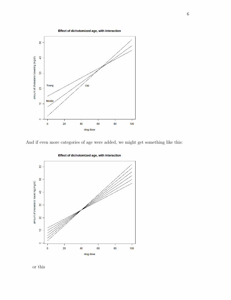
6

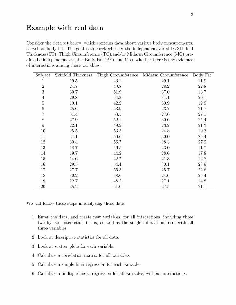
And if even more categories of age were added, we might get something like this:

or this

7

Now imagine adding finer and finer age categories, slowly transforming the age vari-able from discrete (categorical) into a continuous variable. At the limit where agebecomes continuous, we would have an infinite number of different slopes for the effectof dose, one slope for each of the infinite possible age values. This is what we havewhen we have a model with two continuous variables that interact with each other.

The model we would then have would look like this:

Y = α + β1 ∗ dose + β2 × age + β3 × dose ∗ age

For any fixed value of age, say age0, notice that the effect for dose is given by

β1 + β3 ∗ age0

This means that the effect of dose changes depending on the age of the subject, sothat there is really no “unique” effect of dose, it is different for each possible agevalue.

For example, for someone aged 50, the effect of dose is

β1 + 50× β3

8

and for someone aged 30.5 it is:

β1 + 30.5× β3

and so on.

The effect of age is similarly affected by dose. If the dose is, say, dose0, then the effectof age becomes:

β2 + dose0 × β3

In summary: When there is an interaction term, the effect of one variable that formsthe interaction depends on the level of the other variable in the interaction.

Although not illustrated in the above examples, there could always be further vari-ables in the model that are not interacting.

Interactions between two dichotomous variables

Another situation when there can be an interaction between two variables is whenboth variables are dichotomous. Suppose there are two medications, A and B, andeach is given to both males and females. If the medication may operate differentlyin males and females, the equation with interaction term can be written as (supposecoding is Med A = 0, Med B =1, Male = 0, Female=1):

Y = α + β1 ∗med + β2 × sex + β3 ×med ∗ sex

Here, however, there are only four possibilities, as given in the table below:

Case details Mean outcome for that caseMale on Med A αMale on Med B α + β1

Female on Med A α + β2

Female on Med B α + β1 + β2 + β3

Without an interaction term, the mean value for Females on Med B would have beenα+β1 +β2. This implies a simple additive model, as we add the effect of beng femaleto the effect of being on med B. However, with the interaction term as detailed above,the mean value for Females on Med B is α + β1 + β2 + β3, implying that over andabove the additive effect, there is an interaction effect of size β3 .

9

Example with real data

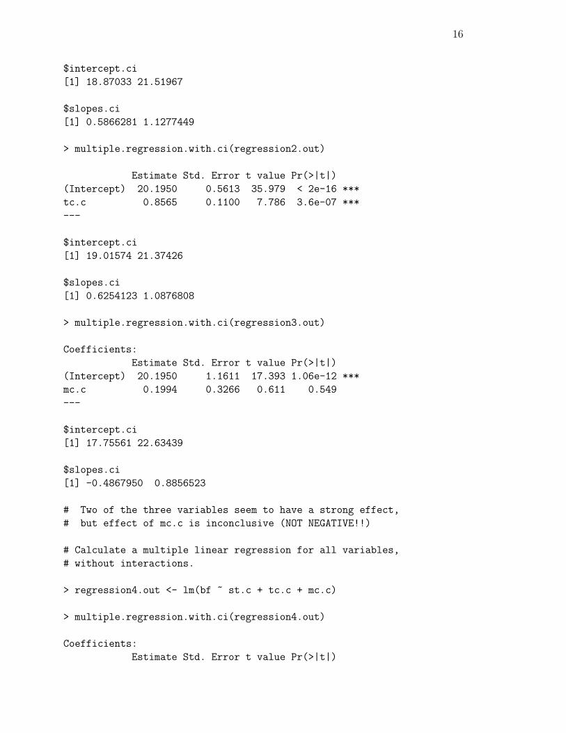
Consider the data set below, which contains data about various body measurements,as well as body fat. The goal is to check whether the independent variables SkinfoldThickness (ST), Thigh Circumference (TC),and/or Midarm Circumference (MC) pre-dict the independent variable Body Fat (BF), and if so, whether there is any evidenceof interactions among these variables.

Subject Skinfold Thickness Thigh Circumference Midarm Circumference Body Fat1 19.5 43.1 29.1 11.92 24.7 49.8 28.2 22.83 30.7 51.9 37.0 18.74 29.8 54.3 31.1 20.15 19.1 42.2 30.9 12.96 25.6 53.9 23.7 21.77 31.4 58.5 27.6 27.18 27.9 52.1 30.6 25.49 22.1 49.9 23.2 21.310 25.5 53.5 24.8 19.311 31.1 56.6 30.0 25.412 30.4 56.7 28.3 27.213 18.7 46.5 23.0 11.714 19.7 44.2 28.6 17.815 14.6 42.7 21.3 12.816 29.5 54.4 30.1 23.917 27.7 55.3 25.7 22.618 30.2 58.6 24.6 25.419 22.7 48.2 27.1 14.820 25.2 51.0 27.5 21.1

We will follow these steps in analysing these data:

1. Enter the data, and create new variables, for all interactions, including threetwo by two interaction terms, as well as the single interaction term with allthree variables.

2. Look at descriptive statistics for all data.

3. Look at scatter plots for each variable.

4. Calculate a correlation matrix for all variables.

5. Calculate a simple liner regression for each variable.

6. Calculate a multiple linear regression for all variables, without interactions.

10

7. Add in various interactions, to see what happens.

8. Draw overall conclusions based on the totality of evidence from all models.

# Enter the data:

> st<-c(19.5, 24.7, 30.7, 29.8, 19.1, 25.6, 31.4, 27.9, 22.1, 25.5, 31.1,

30.4, 18.7, 19.7, 14.6, 29.5, 27.7, 30.2, 22.7, 25.2)

> tc<-c(43.1, 49.8, 51.9, 54.3, 42.2, 53.9, 58.5, 52.1, 49.9, 53.5, 56.6,

56.7, 46.5, 44.2, 42.7, 54.4, 55.3, 58.6, 48.2, 51.0)

> mc<-c(29.1, 28.2, 37.0, 31.1, 30.9, 23.7, 27.6, 30.6, 23.2, 24.8, 30.0,

28.3, 23.0, 28.6, 21.3, 30.1, 25.7, 24.6, 27.1, 27.5)

> bf<-c(11.9, 22.8, 18.7, 20.1, 12.9, 21.7, 27.1, 25.4, 21.3,

19.3, 25.4, 27.2, 11.7, 17.8, 12.8, 23.9, 22.6, 25.4, 14.8,

21.1)

# Create new variables, for all interactions, including three two

# by two interaction terms, as well as the single interaction term

# with all three variables.

> st_tc <- st*tc

> st_mc <- st*mc

> tc_mc <- tc*mc

> st_tc_mc <- st*tc*mc

# Create a data frame with all data:

> fat <- data.frame(st, tc, mc, st_tc, st_mc, tc_mc, st_tc_mc, bf)

# Look at the data

> fat

st tc mc st_tc st_mc tc_mc st_tc_mc bf

1 19.5 43.1 29.1 840.45 567.45 1254.21 24457.10 11.9

2 24.7 49.8 28.2 1230.06 696.54 1404.36 34687.69 22.8

3 30.7 51.9 37.0 1593.33 1135.90 1920.30 58953.21 18.7

4 29.8 54.3 31.1 1618.14 926.78 1688.73 50324.15 20.1

5 19.1 42.2 30.9 806.02 590.19 1303.98 24906.02 12.9

6 25.6 53.9 23.7 1379.84 606.72 1277.43 32702.21 21.7

11

7 31.4 58.5 27.6 1836.90 866.64 1614.60 50698.44 27.1

8 27.9 52.1 30.6 1453.59 853.74 1594.26 44479.85 25.4

9 22.1 49.9 23.2 1102.79 512.72 1157.68 25584.73 21.3

10 25.5 53.5 24.8 1364.25 632.40 1326.80 33833.40 19.3

11 31.1 56.6 30.0 1760.26 933.00 1698.00 52807.80 25.4

12 30.4 56.7 28.3 1723.68 860.32 1604.61 48780.14 27.2

13 18.7 46.5 23.0 869.55 430.10 1069.50 19999.65 11.7

14 19.7 44.2 28.6 870.74 563.42 1264.12 24903.16 17.8

15 14.6 42.7 21.3 623.42 310.98 909.51 13278.85 12.8

16 29.5 54.4 30.1 1604.80 887.95 1637.44 48304.48 23.9

17 27.7 55.3 25.7 1531.81 711.89 1421.21 39367.52 22.6

18 30.2 58.6 24.6 1769.72 742.92 1441.56 43535.11 25.4

19 22.7 48.2 27.1 1094.14 615.17 1306.22 29651.19 14.8

20 25.2 51.0 27.5 1285.20 693.00 1402.50 35343.00 21.1

# Look at descriptive statistics for all data.

> summary(fat)

st tc mc st_tc

Min. :14.60 Min. :42.20 Min. :21.30 Min. : 623.4

1st Qu.:21.50 1st Qu.:47.77 1st Qu.:24.75 1st Qu.:1038.3

Median :25.55 Median :52.00 Median :27.90 Median :1372.0

Mean :25.31 Mean :51.17 Mean :27.62 Mean :1317.9

3rd Qu.:29.90 3rd Qu.:54.63 3rd Qu.:30.02 3rd Qu.:1608.1

Max. :31.40 Max. :58.60 Max. :37.00 Max. :1836.9

st_mc tc_mc st_tc_mc bf

Min. : 311.0 Min. : 909.5 Min. :13279 Min. :11.70

1st Qu.: 584.5 1st Qu.:1274.1 1st Qu.:25415 1st Qu.:17.05

Median : 694.8 Median :1403.4 Median :35015 Median :21.20

Mean : 706.9 Mean :1414.9 Mean :36830 Mean :20.20

3rd Qu.: 861.9 3rd Qu.:1607.1 3rd Qu.:48423 3rd Qu.:24.27

Max. :1135.9 Max. :1920.3 Max. :58953 Max. :27.20

# Look at scatter plots for each variable.

> pairs(fat)

12

# Calculate a correlation matrix for all variables.

> cor(fat)

st tc mc st_tc st_mc tc_mc

st 1.0000000 0.9238425 0.4577772 0.9887843 0.9003214 0.8907135

tc 0.9238425 1.0000000 0.0846675 0.9663436 0.6719665 0.6536065

mc 0.4577772 0.0846675 1.0000000 0.3323920 0.7877028 0.8064087

st_tc 0.9887843 0.9663436 0.3323920 1.0000000 0.8344518 0.8218605

st_mc 0.9003214 0.6719665 0.7877028 0.8344518 1.0000000 0.9983585

tc_mc 0.8907135 0.6536065 0.8064087 0.8218605 0.9983585 1.0000000

st_tc_mc 0.9649137 0.8062687 0.6453482 0.9277172 0.9778029 0.9710983

bf 0.8432654 0.8780896 0.1424440 0.8697087 0.6339052 0.6237307

st_tc_mc bf

0.9649137 0.8432654

0.8062687 0.8780896

0.6453482 0.1424440

13

0.9277172 0.8697087

0.9778029 0.6339052

0.9710983 0.6237307

1.0000000 0.7418017

0.7418017 1.0000000

Looking at the scatter plots and correlation matrix, we see trouble. Many of thecorrelations between the independent variables are very high, which will cause severeconfounding and/or near collinearity. The problem is particularly acute among theinteraction variables we created.

Trick that sometimes helps: Subtract the mean from each independent variable,and use these so-called “centered” variables to create the interaction variables.

This will not change the correlations among the non-interaction terms, but may reducecorrelations for interaction terms.

# Create the centered independent variables:

> st.c <- st - mean(st)

> tc.c <- tc - mean(tc)

> mc.c <- mc - mean(mc)

# Now create the centered interaction terms:

> st_tc.c <- st.c*tc.c

> st_mc.c <- st.c*mc.c

> tc_mc.c <- tc.c*mc.c

> st_tc_mc.c <- st.c*tc.c*mc.c

# Create a new data frame with this new set of independent variables

fat.c <- data.frame(st.c, tc.c, mc.c, st_tc.c, st_mc.c, tc_mc.c, st_tc_mc.c, bf)

> fat.c

st.c tc.c mc.c st_tc.c st_mc.c tc_mc.c st_tc_mc.c bf

1 -5.805 -8.07 1.48 46.84635 -8.5914 -11.9436 69.332598 11.9

2 -0.605 -1.37 0.58 0.82885 -0.3509 -0.7946 0.480733 22.8

3 5.395 0.73 9.38 3.93835 50.6051 6.8474 36.941723 18.7

4 4.495 3.13 3.48 14.06935 15.6426 10.8924 48.961338 20.1

5 -6.205 -8.97 3.28 55.65885 -20.3524 -29.4216 182.561028 12.9

6 0.295 2.73 -3.92 0.80535 -1.1564 -10.7016 -3.156972 21.7

7 6.095 7.33 -0.02 44.67635 -0.1219 -0.1466 -0.893527 27.1

8 2.595 0.93 2.98 2.41335 7.7331 2.7714 7.191783 25.4

14

9 -3.205 -1.27 -4.42 4.07035 14.1661 5.6134 -17.990947 21.3

10 0.195 2.33 -2.82 0.45435 -0.5499 -6.5706 -1.281267 19.3

11 5.795 5.43 2.38 31.46685 13.7921 12.9234 74.891103 25.4

12 5.095 5.53 0.68 28.17535 3.4646 3.7604 19.159238 27.2

13 -6.605 -4.67 -4.62 30.84535 30.5151 21.5754 -142.505517 11.7

14 -5.605 -6.97 0.98 39.06685 -5.4929 -6.8306 38.285513 17.8

15 -10.705 -8.47 -6.32 90.67135 67.6556 53.5304 -573.042932 12.8

16 4.195 3.23 2.48 13.54985 10.4036 8.0104 33.603628 23.9

17 2.395 4.13 -1.92 9.89135 -4.5984 -7.9296 -18.991392 22.6

18 4.895 7.43 -3.02 36.36985 -14.7829 -22.4386 -109.836947 25.4

19 -2.605 -2.97 -0.52 7.73685 1.3546 1.5444 -4.023162 14.8

20 -0.105 -0.17 -0.12 0.01785 0.0126 0.0204 -0.002142 21.1

# Look at the new correlation matrix

> cor(fat.c)

st.c tc.c mc.c st_tc.c st_mc.c tc_mc.c

st.c 1.0000000 0.9238425 0.45777716 -0.4770137 -0.17341554 -0.2215706

tc.c 0.9238425 1.0000000 0.08466750 -0.4297883 -0.17253677 -0.1436553

mc.c 0.4577772 0.0846675 1.00000000 -0.2158921 -0.03040675 -0.2353658

st_tc.c -0.4770137 -0.4297883 -0.21589210 1.0000000 0.23282905 0.2919073

st_mc.c -0.1734155 -0.1725368 -0.03040675 0.2328290 1.00000000 0.8905095

tc_mc.c -0.2215706 -0.1436553 -0.23536583 0.2919073 0.89050954 1.0000000

st_tc_mc.c 0.4241959 0.2054264 0.62212493 -0.4975292 -0.67215024 -0.7398958

bf 0.8432654 0.8780896 0.14244403 -0.3923247 -0.25113314 -0.1657072

st_tc_mc.c bf

0.4241959 0.8432654

0.2054264 0.8780896

0.6221249 0.1424440

-0.4975292 -0.3923247

-0.6721502 -0.2511331

-0.7398958 -0.1657072

1.0000000 0.2435352

0.2435352 1.0000000

Still not perfect, but notice that the correlations have been drastically reduced forsome of the interaction variables.

Why does this work? Consider two variables that are highly correlated:

> x<- 1:10

> x2 <- x^2

> cor(x,x2)

15

[1] 0.9745586

> plot(x,x2)

> x.c <- x-mean(x)

> x2.c <- x.c^2

> cor(x.c, x2.c)

[1] 0

> plot(x.c, x2.c)

By “balancing” positive and negative values, correlations are reduced. We will startlooking at the regressions.

# Calculate a simple linear regression for each variable (not the

interactions).

> regression1.out <- lm(bf ~ st.c)

> regression2.out <- lm(bf ~ tc.c)

> regression3.out <- lm(bf ~ mc.c)

> multiple.regression.with.ci(regression1.out)

Estimate Std. Error t value Pr(>|t|)

(Intercept) 20.1950 0.6305 32.029 < 2e-16 ***

st.c 0.8572 0.1288 6.656 3.02e-06 ***

---

16

$intercept.ci

[1] 18.87033 21.51967

$slopes.ci

[1] 0.5866281 1.1277449

> multiple.regression.with.ci(regression2.out)

Estimate Std. Error t value Pr(>|t|)

(Intercept) 20.1950 0.5613 35.979 < 2e-16 ***

tc.c 0.8565 0.1100 7.786 3.6e-07 ***

---

$intercept.ci

[1] 19.01574 21.37426

$slopes.ci

[1] 0.6254123 1.0876808

> multiple.regression.with.ci(regression3.out)

Coefficients:

Estimate Std. Error t value Pr(>|t|)

(Intercept) 20.1950 1.1611 17.393 1.06e-12 ***

mc.c 0.1994 0.3266 0.611 0.549

---

$intercept.ci

[1] 17.75561 22.63439

$slopes.ci

[1] -0.4867950 0.8856523

# Two of the three variables seem to have a strong effect,

# but effect of mc.c is inconclusive (NOT NEGATIVE!!)

# Calculate a multiple linear regression for all variables,

# without interactions.

> regression4.out <- lm(bf ~ st.c + tc.c + mc.c)

> multiple.regression.with.ci(regression4.out)

Coefficients:

Estimate Std. Error t value Pr(>|t|)

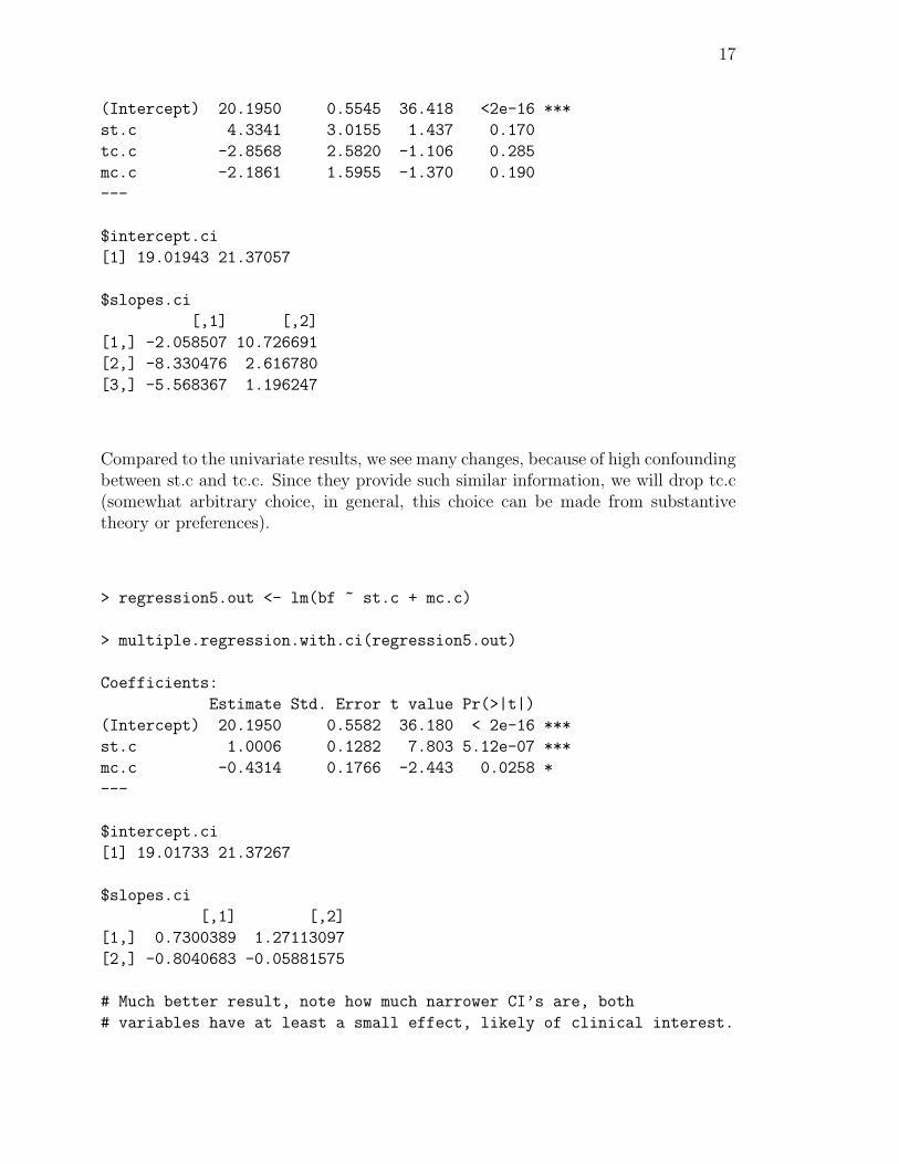
17

(Intercept) 20.1950 0.5545 36.418 <2e-16 ***

st.c 4.3341 3.0155 1.437 0.170

tc.c -2.8568 2.5820 -1.106 0.285

mc.c -2.1861 1.5955 -1.370 0.190

---

$intercept.ci

[1] 19.01943 21.37057

$slopes.ci

[,1] [,2]

[1,] -2.058507 10.726691

[2,] -8.330476 2.616780

[3,] -5.568367 1.196247

Compared to the univariate results, we see many changes, because of high confoundingbetween st.c and tc.c. Since they provide such similar information, we will drop tc.c(somewhat arbitrary choice, in general, this choice can be made from substantivetheory or preferences).

> regression5.out <- lm(bf ~ st.c + mc.c)

> multiple.regression.with.ci(regression5.out)

Coefficients:

Estimate Std. Error t value Pr(>|t|)

(Intercept) 20.1950 0.5582 36.180 < 2e-16 ***

st.c 1.0006 0.1282 7.803 5.12e-07 ***

mc.c -0.4314 0.1766 -2.443 0.0258 *

---

$intercept.ci

[1] 19.01733 21.37267

$slopes.ci

[,1] [,2]

[1,] 0.7300389 1.27113097

[2,] -0.8040683 -0.05881575

# Much better result, note how much narrower CI’s are, both

# variables have at least a small effect, likely of clinical interest.

18

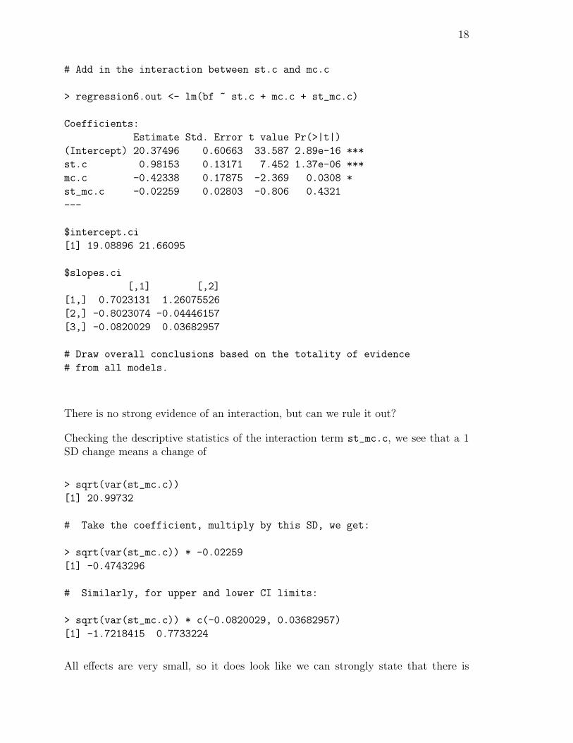
# Add in the interaction between st.c and mc.c

> regression6.out <- lm(bf ~ st.c + mc.c + st_mc.c)

Coefficients:

Estimate Std. Error t value Pr(>|t|)

(Intercept) 20.37496 0.60663 33.587 2.89e-16 ***

st.c 0.98153 0.13171 7.452 1.37e-06 ***

mc.c -0.42338 0.17875 -2.369 0.0308 *

st_mc.c -0.02259 0.02803 -0.806 0.4321

---

$intercept.ci

[1] 19.08896 21.66095

$slopes.ci

[,1] [,2]

[1,] 0.7023131 1.26075526

[2,] -0.8023074 -0.04446157

[3,] -0.0820029 0.03682957

# Draw overall conclusions based on the totality of evidence

# from all models.

There is no strong evidence of an interaction, but can we rule it out?

Checking the descriptive statistics of the interaction term st_mc.c, we see that a 1SD change means a change of

> sqrt(var(st_mc.c))

[1] 20.99732

# Take the coefficient, multiply by this SD, we get:

> sqrt(var(st_mc.c)) * -0.02259

[1] -0.4743296

# Similarly, for upper and lower CI limits:

> sqrt(var(st_mc.c)) * c(-0.0820029, 0.03682957)

[1] -1.7218415 0.7733224

All effects are very small, so it does look like we can strongly state that there is

19

no interaction here. Had the CI been wider and included clinically interesting ef-fects, it would have been inconclusive (this is extremely common when investigatinginteractions).

Final Comments

• We have looked only at “first order” interactions, and only at interactions be-tween two variables at a time. However, second order interactions, or interac-tions between three or more variables are also possible.

• For example, it is not difficult to find situations where one independent X1

variable may be related to an outcome Y say with a quadratic term, and, atthe same time, this variable interactions with another continuous or indicatorvariable, say Z. For example, we may have an equation like this:

Y = α + β1X + β2X2 + β3Z + β4XZ + β5X

2Z

or more simply

Y = α + β1X + β2X2 + β3Z + β4XZ

• As another example, there may be three variables which all interact with eachother. A possible equation may then look like this:

Y = α + β1X + β2W + β3Z + β4XWZ

• This can become even more complicated if both two and three variable interac-tions co-exist. For example, we may have an equation like this:

Y = α + β1X + β2W + β3Z + β4XWZ + β5XW + β6XZ + β7WZ

or

Y = α + β1X + β2W + β3Z + β4XWZ + β5XW + β6XZ

and so on.

• In all of the above cases, the principles detailed above for simpler interactionsapply.

• A general practical problem with all interactions is that they can be hard todetect in small or moderately sized data sets, i.e., the confidence intervals for theinteraction term β coefficients will be very wide, and thus inconclusive. Thereis not much that can be done about this at the analysis stage of a study, but ifyou are planning a study you can try to ensure a large enough sample size, andmeasure all variables as accurately as possible.