3.1 Introduction

The previous chapter has provided some insight into the basic measurements that arenecessary for inertial navigation. For the purposes of the ensuing discussion, it isassumed that measurements of specific force and angular rate are available alongand about axes which are mutually perpendicular. Attention is focused on how thesemeasurements are combined and processed to enable navigation to take place.

3.2 A simple two-dimensional strapdown navigation system

We begin this chapter by describing a simplified two-dimensional strapdown navi-gation system. Although functionally identical to the full three-dimensional systemdiscussed later, the computational processes which must be implemented to performthe navigation task in two dimensions are much simplified compared with a fullstrapdown system. Therefore, through this introductory discussion, it is hoped toprovide the reader with an appreciation of the basic processing tasks which must beimplemented in a strapdown system without becoming too deeply involved in theintricacies and complexities of the full system computational tasks.

For the purposes of this discussion, it is assumed that a system is required tonavigate a vehicle which is constrained to move in a single plane. A two-dimensionalstrapdown system capable of fulfilling this particular navigation task was introducedvery briefly in Chapter 2 and is shown diagrammatically in Figure 3.1.

The system contains two accelerometers and a single axis rate gyroscope, all ofwhich are attached rigidly to the body of the vehicle. The vehicle body is represented,in the figure, by the block on which the instruments shown are mounted. The sen-sitive axes of the accelerometers, indicated by the directions of the arrows in thediagram, are at right angles to one another and aligned with the body axes of the

Chapter 3

Basic principles of strapdown inertialnavigation systems

Figure 3.2 Reference frames for two-dimensional navigation

vehicle in the plane of motion; they are denoted as the x\> and Zh axes. The gyroscopeis mounted with its sensitive axis orthogonal to both accelerometer axes allowing itto detect rotations about an axis perpendicular to the plane of motion; the Vb axis. It isassumed that navigation is required to take place with respect to a space-fixed refer-ence frame denoted by the axes X1 and z\. The reference and body axis sets are shownin Figure 3.2, where 0 represents the angular displacement between the body andreference frames.

Figure 3.1 Two-dimensional strapdown inertial navigation system

Key:Sensitive axis

Resolution

Integration

Accelerometer

Gyroscope

Figure 3.3 Two-dimensional strapdown navigation system equations

Referring now to Figure 3.1, body attitude, #, is computed by integrating themeasured angular rate, co b, with respect to time. This information is then usedto resolve the measurements of specific force, fx\> and /zb, into the reference frame.A gravity model, stored in the computer, is assumed to provide estimates of the gravitycomponents in the reference frame, gx{ and gz{. These quantities are combined with theresolved measurements of specific force, fx{ and / z i , to determine true accelerations,denoted by vx\ and vz\. These derivatives are subsequently integrated twice to obtainestimates of vehicle velocity and position. The full set of equations which must besolved are given in Figure 3.3.

Having defined the basic functions which must be implemented in a strapdowninertial navigation system, consideration is now given to the application of the two-dimensional system, described above, for navigation in a rotating reference frame.For instance, consider the situation where it is required to navigate a vehicle moving ina meridian plane around the Earth, as depicted in Figure 3.4. Hence, we are concernedhere with a system which is operating in the vertical plane alone. Such a system wouldbe required to provide estimates of velocity with respect to the Earth, position alongthe meridian and height above the Earth.

Whilst the system mechanisation as described could be used to determine suchinformation, this would entail a further transformation of the velocity and position,derived in space fixed coordinates, to a geographic frame. An alternative and oftenused approach is to navigate directly in a local geographic reference frame, defined inthis simplified case by the direction of the local vertical at the current location of thevehicle. In order to provide the required navigation information, it now becomes nec-essary to keep track of vehicle attitude with respect to the local geographic framedenoted by the axes x and z. This information can be extracted by differencingthe successive gyroscopic measurements of body turn rate with respect to inertialspace, and the current estimate of the turn rate of the reference frame with respectto inertial space. For a vehicle moving at a velocity, Vx, in a single plane around aperfectly spherical Earth of radius Ro9 this rate is given by vx/(Ro + z) where z is theheight of the vehicle above the surface of the Earth. This is often referred to as thetransport rate.

Figure 3.5 Simplified two-dimensional strapdown system equations for navigationin a rotating reference frame

Figure 3.4 shows a modified two-dimensional strapdown system for navigationin the moving reference frame. As shown in the figure, an estimate of the turnrate of the reference frame is derived using the estimated component of horizontalvelocity.

The equations which must be solved in this system are given in Figure 3.5.Comparison with the equations given in Figure 3.3, relating to navigation with

respect to a space-fixed axis set, reveals the following differences. The attitude com-putation is modified to take account of the turn rate of the local vertical reference frame

Key:Sensitive axisResolution

Integration

Summingjunction

Accelerometer

Gyroscope

Earth's surfaceEarth'sradius R0

Figure 3.4 Two-dimensional strapdown inertia! system for navigation in a rotatingreference frame

as described above. Consequently, the equation in 0 is modified by the subtractionof the term Vx/(RQ + z) in Figure 3.4. The terms vxvz/(Ro + z) and v*/(Ro + z)which appear in the velocity equations are included to take account of the addi-tional forces acting as the system moves around the Earth (Coriolis forces, seeSection 3.4). The gravity term (g) appears only in the vz equation as it is assumedthat the Earth's gravitational acceleration acts precisely in the direction of the localvertical.

This section has outlined the basic form of the computing tasks to be implementedin a strapdown navigation system using a much simplified two-dimensional repre-sentation. In the remainder of this chapter the extension of this simple strapdownsystem to three dimensions is described in some detail. It will be appreciated thatthis entails a substantial increase in the complexity of the computing tasks involved.In particular, attitude information in three dimensions can no longer be obtained bya simple integration of the measured turn rates.

3.3 Reference frames

Fundamental to the process of inertial navigation is the precise definition of a numberof Cartesian co-ordinate reference frames. Each frame is an orthogonal, right-handed,co-ordinate frame or axis set.

For navigation over the Earth, it is necessary to define axis sets which allowthe inertial measurements to be related to the cardinal directions of the Earth, that is,frames which have a physical significance when attempting to navigate in the vicinityof the Earth. Therefore, it is customary to consider an inertial reference frame which isstationary with respect to the fixed stars, the origin of which is located at the centre ofthe Earth. Such a reference frame is shown in Figure 3.6, together with an Earth-fixedreference frame and a local geographic navigation frame defined for the purposes ofterrestrial inertial navigation.

The following co-ordinate frames are used in the text:

The inertial frame (i-frame) has its origin at the centre of the Earth and axes whichare non-rotating with respect to the fixed stars, defined by the axes Ojq, Oy1, Ozj,with OZi coincident with the Earth's polar axis (which is assumed to be invariantin direction).

The Earth frame (e-frame) has its origin at the centre of the Earth and axes which arefixed with respect to the Earth, defined by the axes Ojce, Ove, Oze with Oze alongthe Earth's polar axis. The axis Oxe lies along the intersection of the plane of theGreenwich meridian with the Earth's equatorial plane. The Earth frame rotates,with respect to the inertial frame, at a rate £2 about the axis Ozi.

The navigation frame (n-frame) is a local geographic frame which has its origin atthe location of the navigation system, point P, and axes aligned with the directionsof north, east and the local vertical (down). The turn rate of the navigation frame,with respect to the Earth-fixed frame, ooen, is governed by the motion of the pointP with respect to the Earth. This is often referred to as the transport rate.

Greenwichmeridian

lnertialaxes

Localgeographic/navigation

axes

Localmeridian

plane

Equatorialplane

Figure 3.6 Frames of reference

Figure 3.7 Illustration of a body reference frame

The wander azimuth frame (w-frame) may be used to avoid the singularities in thecomputation which occur at the poles of the navigation frame. Like the navigationframe, it is locally level but is rotated through the wander angle about the localvertical. Its use is described in Section 3.5.

The body frame (b-frame), depicted in Figure 3.7, is an orthogonal axis set which isaligned with the roll, pitch and yaw axes of the vehicle in which the navigationsystem is installed.

3.4 Three-dimensional strapdown navigation system - general analysis

3.4.1 Navigation with respect to a fixed frame

Consider the situation where it is required to navigate with respect to a fixed, ornon-accelerating, and non-rotating set of axes. The measured components of specific

Earthaxes

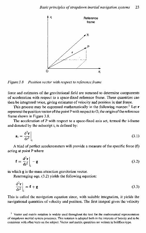
Figure 3.8 Position vector with respect to reference frame

force and estimates of the gravitational field are summed to determine componentsof acceleration with respect to a space-fixed reference frame. These quantities canthen be integrated twice, giving estimates of velocity and position in that frame.

This process may be expressed mathematically in the following manner.1 Let rrepresent the position vector of the point P with respect to O, the origin of the referenceframe shown in Figure 3.8.

The acceleration of P with respect to a space-fixed axis set, termed the i-frameand denoted by the subscript i, is defined by:

d2r

A triad of perfect accelerometers will provide a measure of the specific force (f)acting at point P where

d2rf=wrg (3-2)in which g is the mass attraction gravitation vector.

Rearranging eqn. (3.2) yields the following equation:

d2r

d?r f+g (3-3)

This is called the navigation equation since, with suitable integration, it yields thenavigational quantities of velocity and position. The first integral gives the velocity

1 Vector and matrix notation is widely used throughout the text for the mathematical representationof strapdown inertial system processes. This notation is adopted both in the interests of brevity and to beconsistent with other texts on the subject. Vector and matrix quantities are written in boldface type.

Referenceframe

of point P with respect to the i-frame, viz.

(3.4)

whilst a second integration gives its position in that frame.

3.4.2 Navigation with respect to a rotating frame

In practice, one often needs to derive estimates of a vehicle's velocity and positionwith respect to a rotating reference frame, as when navigating in the vicinity of theEarth. In this situation, additional apparent forces will be acting which are functionsof reference frame motion. This results in a revised form of the navigation equationwhich may be integrated to determine the ground speed of the vehicle, ve, directly.Alternatively, ve may be computed from the inertial velocity, Vi, using the theoremof Coriolis, as follows,

(3.5)

where (Oje = [0 0 Q]T is the turn rate of the Earth frame with respect to the i-frameand x denotes a vector cross product.

Revised forms of the navigation equation suitable for navigation with respect tothe Earth are the subject of Section 3.5.

3.4.3 The choice of reference frame

The navigation equation, eqn. (3.3), may be solved in any one of a number of referenceframes. If the Earth frame is chosen, for example, then the solution of the navigationequation will provide estimates of velocity with respect to either the inertial frame orthe Earth frame, expressed in Earth coordinates, denoted v? and v^, respectively.2

In Section 3.5, a number of different strapdown system mechanisations fornavigating with respect to the Earth are described. In each case, it will be shownthat the navigation equation is expressed in a different manner depending on thechoice of reference frame.

3.4.4 Resolution of accelerometer measurements

The accelerometers usually provide a measurement of specific force in a body fixedaxis set, denoted fb. In order to navigate, it is necessary to resolve the components ofthe specific force in the chosen reference frame. In the event that the inertial frameis selected, this may be achieved by pre-multiplying the vector quantity fb by thedirection cosine matrix, C^, using,

f1 = C{,fb (3.6)

2 Superscripts attached to vector quantities denote the axis set in which the vector quantity coordinatesare expressed.

where Cj5 is a 3 x 3 matrix which defines the attitude of the body frame with respectto the i-frame. The direction cosine matrix CJ5 may be calculated from the angularrate measurements provided by the gyroscopes using the following equation:

(3.7)

where ^Jj5 is the skew symmetric matrix:

(3.8)

This matrix is formed from the elements of the vector G)-J5 = [p q r ]T whichrepresents the turn rate of the body with respect to the i-frame as measured by thegyroscopes. Equation (3.7) is derived in Section 3.6.

The attitude of the body with respect to the chosen reference frame, which isrequired to resolve the specific force measurements into the reference frame, may bedefined in a number of different ways. For the purposes of the discussion of navigationsystem mechanisations in this and the following section, the direction cosine methodwill be adopted. Direction cosines and some alternative attitude representations aredescribed in some detail in Section 3.6.

3.4.5 System example

Consider the situation in which it is required to navigate with respect to inertial spaceand the solution of the navigation takes place in the i-frame. Equation (3.3) may beexpressed in i-frame coordinates as follows:

(3.9)

It is clear from the preceding discussion that the integration of the navigationequation involves the use of information from both the gyroscopes and theaccelerometers contained within the inertial navigation system. A block diagramrepresentation of the resulting navigation system is given in Figure 3.9.

The diagram displays the main functions to be implemented within a strapdownnavigation system; the processing of the rate measurements to generate body attitude,the resolution of the specific force measurements into the inertial reference frame,gravity compensation and the integration of the resulting acceleration estimates todetermine velocity and position.

3.5 Strapdown system mechanisations

Attention is focused here on inertial systems which may be used to navigate in thevicinity of the Earth. It has been shown in Section 3.4 how estimates of positionand velocity are derived by integrating a navigation equation of the form given in

Bodymounted

accelerometers

Resolutionof

specific forcemeasurements

Gravitycomputer

Navigationcomputer Position

and velocity (V1)estimates

Bodymounted

gyroscopes

Attitudecomputer

Initial estimates ofvelocity and position

Initial estimates ofattitude

Figure 3.9 Strapdown inertial navigation system

eqn. (3.3). In systems of the type described later, in which it is required to deriveestimates of vehicle velocity and position with respect to an Earth fixed frame, addi-tional apparent forces will be acting which are functions of the reference frame motion.In this section, further forms of the navigation equation are derived, correspondingto different choices of reference frame [I].

The resulting system mechanisations are described together with their appli-cations. As will become apparent, the variations in the mechanisations describedhere are in the strapdown computational algorithms and not in the arrangement ofthe sensors or the mechanical layout of the system.

3.5.1 Inertial frame mechanisation

In this system, it is required to calculate vehicle speed with respect to the Earth, theground speed, in inertial axes, denoted by the symbol v^. This may be accomplishedby expressing the navigation equation (eqn. (3.3)) in inertial axes and deriving anexpression for ^ f |e in terms of ground speed and its time derivatives with respect tothe inertial frame.

Inertial velocity may be expressed in terms of ground speed using the Coriolisequation, viz.

(3.10)

Differentiating this expression and writing ^ |e = ve, we have,

(3.11)

Applying the Coriolis equation in the form of eqn. (3.10) to the second term ineqn. (3.11) gives:

(3.12)

In generating the above equation, it is assumed that the turn rate of the Earth isconstant, hence ^ ^ = 0.

Combining eqns. (3.3) and (3.12) and rearranging yields:

(3.13)

In this equation, f represents the specific force acceleration to which the navigationsystem is subjected, while coie x ve is the acceleration caused by its velocity over thesurface of a rotating Earth, usually referred to as the Coriolis acceleration. The term(Oie x [coie x r], in eqn. (3.13), defines the centripetal acceleration experienced by thesystem owing to the rotation of the Earth, and is not separately distinguishable fromthe gravitational acceleration which arises through mass attraction, g. The sum of theaccelerations caused by the mass attraction force and the centripetal force constituteswhat is known as the local gravity vector, the vector to which a 'plumb bob' wouldalign itself when held above the Earth (Figure 3.10). This is denoted here by thesymbol gi, that is:

(3.14)

Earth's rate

Localgravityvector

Gravitational field intensityat point P

Figure 3.10 Diagram showing the components of the gravitational field

Combining eqns. (3.13) and (3.14) gives the following form of the navigationequation:

(3.15)

This equation may be expressed in inertial axes, as follows, using the superscriptnotation mentioned earlier.

(3.16)

The measurements of specific force provided by the accelerometers are in body axes,as denoted by the vector quantity fb. In order to set up the navigation eqn. (3.16),the accelerometer outputs must be resolved into inertial axes to give f1. This may beachieved by pre-multiplying the measurement vector fb by the direction cosine matrixC^ as described in Section 3.4.4 (eqn. (3.6)). Given knowledge of the attitude of thebody at the start of navigation, the matrix C^ is updated using eqns. (3.7) and (3.8)based on measurements of the body rates with respect to the i-frame which may beexpressed as follows:

(3.17)

Substituting for f1 from eqn. (3.6) in eqn. (3.16) gives the following form of thenavigation equation:

(3.18)

The final term in this equation represents the local gravity vector expressed in theinertial frame.

A block diagram representation of the resulting inertial frame mechanisation isshown in Figure 3.11.

3.5.2 Earth frame mechanisation

In this system, ground speed is expressed in an Earth-fixed co-ordinate frame togive V®. It follows from the Coriolis equation, that the rate of change of ve, withrespect to Earth axes, may be expressed in terms of its rate of change in inertial axesusing:

(3.19)

Substituting for ^ - 1 1 from eqn. (3.15), we have:

(3.20)

Bodymounted

accelerometers

Bodymounted

gyroscopes

Resolutionof

specific forcemeasurements

Attitudecomputer

Initial estimates ofvelocity and position

Positionand velocity (v^)

estimates

Initial estimates ofattitude

Figure 3.11 Strapdown inertia! navigation system - inertial frame mechanisation

This may be expressed in Earth axes as follows:

(3.21)

where C£ is the direction cosine matrix used to transform the measured specificforce vector into Earth axes. This matrix propagates in accordance with the followingequation:

(3.22)

where Q^ is the skew symmetric form of O)J , the body rate with respect to theEarth-fixed frame. This is derived by differencing the measured body rates, Gt)Jj5,and estimates of the components of Earth's rate, <*)ie, expressed in body axes asfollows:

(3.23)

in which Cg = C£T, the transpose of the matrix C£.A block diagram representation of the Earth frame mechanisation is shown in

Figure 3.12.A variation on this system may be used when it is required to navigate over

relatively short distances, with respect to a fixed point on the Earth. A mechanisa-tion of this type may be used for a tactical missile application in which navigationis required with respect to a ground based tracking station. In such a system,

Gravitycomputer

Positioninformation

Corioliscorrection

Navigationcomputer

Figure 3.12 Strapdown inertial navigation system - Earth frame mechanisation

target tracking information provided by the ground station may need to be com-bined with the outputs of an on-board inertial navigation system to provide missilemid-course guidance commands. In order that the missile may operate in harmonywith the ground systems, all information must be provided in a common frame ofreference.

In this situation, an Earth-fixed reference frame may be defined, the origin ofwhich is located at the tracking station, its axes aligned with the local vertical anda plane which is tangential to the Earth's surface, as illustrated in Figure 3.13.

For very short term navigation, as required for some tactical missile applications,further simplifications to this system mechanisation may be permitted. For instance,where the navigation period is short, typically 10 minutes or less, the effects of therotation of the Earth on the attitude computation process can sometimes be ignored,and Coriolis corrections are no longer essential in the velocity equation to givesufficiently accurate navigation. In this situation, attitude is computed solely as afunction of the turn rates measured by the gyroscopes, and eqn. (3.21) reduces tothe following:

*e = Cgfb + gf (3.24)

It is stressed, that such simplifications can only be allowed in cases where thenavigation errors, induced by the omission of Earth rate and Coriolis terms, lie withinthe error bounds in which the navigation system is required to operate. This situationarises when the permitted gyroscopic errors are in excess of the rotation rate of theEarth, and allowable accelerometer biases are in excess of the acceleration errorsintroduced by ignoring the Coriolis forces.

Bodymounted

accelerometers

Resolutionof

specific forcemeasurements

Bodymounted

gyroscopes

Gravitycomputer

Navigationcomputer

Initial estimates ofvelocity and position

Attitudecomputer

Initial estimates ofattitude

Positioninformation

Corioliscorrection

Positionand

velocity (vf)estimates

Figure 3.14 Geographic co-ordinate system

3.5.3 Local geographic navigation frame mechanisation

In order to navigate over large distances around the Earth, navigation informationis most commonly required in the local geographic or navigation axis set describedearlier. Position on the Earth may be specified in terms of latitude (degrees northor south of a datum) and longitude (degrees east or west of a datum). Figure 3.14shows this geographic co-ordinate system on a globe. Lines of constant latitude andlongitude are called parallels and meridians, respectively.

Navigation data are expressed in terms of north and east velocity components,latitude, longitude and height above the Earth. Whilst such information can be

Localvertical

axis

Tangentplaneaxis

Figure 3.13 Tangent plane axis set

True north

Latitude

Meridian linespass through the

polesEquator

Latitude

Longitude

computed using the position estimates provided by the inertial or Earth frame mech-anisations described before, this involves a further transformation of the vectorquantities v^ or v|. Further, difficulties arise in representing the Earth's gravitationalfield precisely in a computer. For these reasons, the navigation frame mechanisation,described here, is often used when navigating around the Earth.

In this mechanisation, ground speed is expressed in navigation coordinates togive Vg. The rate of change of v£ with respect to navigation axes may be expressedin terms of its rate of change in inertial axes as follows:

(3.25)

Substituting for ^p- |i? from eqn. (3.15), we have:

(3.26)

This may be expressed in navigation axes as follows:

(3.27)

where C£ is a direction cosine matrix used to transform the measured specific forcevector into navigation axes. This matrix propagates in accordance with the followingequation.

(3.28)

where ft J is the skew symmetric form of co^b, the body rate with respect to thenavigation frame. This is derived by differencing the measured body rates, G)-J3,and estimates of the components of navigation frame rate, Win. The latter term isobtained by summing the Earth's rate with respect to the inertial frame and the turnrate of the navigation frame with respect to the Earth, that is, (Oin = <0ie + <oen-Therefore,

(3.29)

A block diagram representation of the navigation frame mechanisation is shownin Figure 3.15.

It is instructive to consider the physical significance of the various terms in thenavigation equation (3.27). From this equation, it can be seen that the rate of changeof the velocity, with respect to the surface of the Earth, is made up of the followingterms:

1. The specific force acting on the vehicle, as measured by a triad of accelerometersmounted within it.

2. A correction for the acceleration caused by the vehicle's velocity over the surfaceof a rotating Earth, usually referred to as the Coriolis acceleration. The effectin two dimensions is illustrated in Figure 3.16. As the point P moves away

Localgravityvector

Bodymounted

accelerometers

Resolutionof

specific forcemeasurements

Bodymounted

gyroscopes

Gravitycomputer

Positioninformation

Corioliscorrection

Navigationcomputer

Initial estimates ofvelocity and position

Attitudecomputer

Positionand

velocity (v£)estimates

Initial estimates ofattitude

Figure 3.15 Strapdown inertial navigation system - local geographic navigationframe mechanisation

Figure 3.16 Illustration of the effect of Coriolis acceleration

from the axis of rotation, it traces out a curve in space as a result of the Earth'srotation.

3. A correction for the centripetal acceleration of the vehicle, resulting from itsmotion over the Earth's surface. For instance, a vehicle moving due east over

Dotted line istrajectory requiredto travel from O to Ron a rotating earth

the surface of the Earth will trace out a circular path with respect to inertial axes.To follow this path, the vehicle is subject to a force acting towards the centre ofthe Earth of magnitude equal to the product of its mass, its linear velocity and itsturn rate with respect to the Earth.

4. Compensation for the apparent gravitational force acting on the vehicle. Thisincludes the gravitational force caused by the mass attraction of the Earth, andthe centripetal acceleration of the vehicle resulting from the rotation of the Earth.The latter term arises even if the vehicle is stationary with respect to the Earth,since the path which its follows in space is circular.

A simple example serves to illustrate the importance of the Coriolis effect.Consider a vehicle launched from the north pole with the intention of flying toNew York city. The vehicle is assumed to travel at an average speed of 3600 miles/h.During the flight, of approximately 1 h, the Earth will have rotated by about 15°,a distance of approximately 900 miles at the latitude of New York. Consequently,if no Coriolis correction was made to the on-board inertial guidance system duringthe course of the flight, the vehicle would arrive in the Chicago area rather thanNew York as originally intended.

3.5.4 Wander azimuth navigation frame mechanisation

In the local geographic navigation frame mechanisation described in the previoussection, the n-frame is required to rotate continuously as the system moves over thesurface of the Earth in order to keep its ;c-axis parallel to true north. In order toachieve this condition worldwide, the n-frame must rotate at much greater rates aboutits z-axis as the navigation system moves over the surface of the Earth in the polarregions, compared to the rates required at lower latitudes. This effect is illustratedin Figure 3.17 which shows a polar view of a near polar crossing. It should be clearfrom the diagram that the rate at which the local geographic navigation frame mustrotate about its z-axis in order to maintain the x-axis pointing at the pole becomesvery large, the heading direction slewing rapidly through 180° when moving pastthe pole. In the most extreme case, a direct crossing of the pole, the turn rate becomesinfinite when passing over the pole.

The effect is illustrated mathematically as follows. The turn rate of the navigationframe, the transport rate, may be expressed in component form as:

(3.30)

where UN is the north velocity, v^ the east velocity, Ro the radius of the Earth, L thelatitude and h the height above ground.

It will be seen that the third component of the transport rate becomes indeterminateat the geographic poles.

One way of avoiding the singularity, and so providing a navigation system withworld-wide capability, is to adopt a wander azimuth mechanisation in which thez-component of <*>£n is set to zero. A wander axis system is a locally level frame

x-axis ofnavigation

frame

Latitude 87°

x-axis ofnavigation

frame

Near polarcrossing

trajectory

Figure 3.17 Geographic reference singularity at pole crossings

Local geographic navigation frame Wander azimuth navigation frame

Figure 3.18 Illustration of wander azimuth frame

which moves over the Earth's surface with the vehicle, as depicted in Figure 3.18.However, as the name implies, the azimuth angle between true north and the x-axisof the wander axis frame varies with vehicle position on the Earth. This varia-tion is chosen in order to avoid discontinuities in the orientation of the wander

frame with respect to the Earth as the vehicle passes over either the north or southpoles.

A navigation equation for a wander azimuth system, which is similar in form toeqn. (3.27), may be constructed as follows:

(3.31)

This equation is integrated to generate estimates of vehicle ground speed in the wanderazimuth frame, v^. This is then used to generate the turn rate of the wander framewith respect to the Earth, co^. The direction cosine matrix which relates the wanderframe to the Earth frame, C™, may be updated using the equation

Cr = C S C (3.32)

where £1™W is a skew symmetric matrix formed from the elements of the angular ratevector (o^. This process is implemented iteratively and enables any singularities to beavoided. Further details concerning wander azimuth systems and the mechanisationsdescribed earlier appear in Reference 1.

3.5.5 Summary ofstrapdown system mechanisations

This section has provided outline descriptions of a number of possible strapdowninertial navigation system mechanisations. Further details are given in Reference 1.The choice of mechanisation is dependent on the application. Whilst any of theschemes described may be used for navigation close to the Earth, the local geographicnavigation frame mechanisation is commonly employed for navigation over largedistances. The wander azimuth system provides a world-wide navigation capability.These mechanisations provide navigation data in terms of north and east velocity,latitude and longitude and allow a relatively simple gravity model to be used. Fornavigation over shorter distances, an Earth fixed reference system may be applicable.

3.6 Strapdown attitude representations

3.6.1 Introductory remarks

Consider now ways in which a set of strapdown gyroscopic sensors may be usedto instrument a reference co-ordinate frame within a vehicle which is free to rotateabout any direction. The attitude of the vehicle with respect to the designated referenceframe may be stored as a set of numbers in a computer within the vehicle. The storedattitude is updated as the vehicle rotates using the measurements of turn rate providedby the gyroscopes.

The co-ordinate frames referred to during the course of the discussion whichfollows are orthogonal, right-handed axis sets in which positive rotations about eachaxis are taken to be in a clockwise direction looking along the axis from the origin,as indicated in the Figure 3.19. A negative rotation acts in an opposite sense, that is,in an anti-clockwise direction. This convention is used throughout this book.

Figure 3.19 Definition of axis rotations

It is important to remember that the change in attitude of a body, which issubjected to a series of rotations about different axes, is not only a function of theangles through which it rotates about each of those axes, but the order in which therotations occur. The illustration given in Figure 3.20, although somewhat extreme,shows quite clearly that the order in which a sequence of rotations occurs is mostimportant.

Rotations are defined here with respect to the orthogonal right-handed axis set,Oxyz, indicated in the figure. The sequence of rotations shown in the left half ofthe figure is made up of a 90° pitch, or v-axis rotation, followed by a 90° yaw,or z-axis rotation, and a further pitch rotation of —90°. On completion of thissequence of turns, it can be seen that a net rotation of 90° about the roll (x) axishas taken place. In the right hand figure, the order of the rotations has been reversed.Although the body still ends up with its roll axis aligned in the original direction,it is seen that a net roll rotation of —90° has now taken place. Hence, individualaxis rotations are said to be non-commutative. It is clear that failure to take accountof the order in which rotations arise can lead to a substantial error in the computedattitude.

Various mathematical representations can be used to define the attitude of a bodywith respect to a co-ordinate reference frame. The parameters associated with eachmethod may be stored within a computer and updated as the vehicle rotates usingthe measurements of turn rate provided by the strapdown gyroscopes. Three attituderepresentations are described here, namely:

1. Direction cosines. The direction cosine matrix, introduced in Section 3.5, is a3 x 3 matrix, the columns of which represent unit vectors in body axes projectedalong the reference axes.

2. Euler angles. A transformation from one co-ordinate frame to another is definedby three successive rotations about different axes taken in turn. The Euler anglerepresentation is perhaps one of the simplest techniques in terms of physical

Positivey rotation

Positivex rotation

Positivez rotation

Figure 3.20 Illustration of effect of order of body rotations

appreciation. The three angles correspond to the angles which would be measuredbetween a set of mechanical gimbals,3 which is supporting a stable element,where the axes of the stable element represent the reference frame, and with thebody being attached via a bearing to the outer gimbal.

3. Quaternions. The quaternion attitude representation allows a transformationfrom one co-ordinate frame to another to be effected by a single rotation abouta vector defined in the reference frame. The quaternion is a four-element vec-tor representation, the elements of which are functions of the orientation of thisvector and the magnitude of the rotation.

•* A gimbal is a rigid mechanical frame which is free to rotate about a single-axis to isolate it fromangular motion in that direction. A stable platform can be isolated from body motion if supported by threesuch frames with their axes of rotation nominally orthogonal to each other.

90° Pitch -90° Pitch

90° Yaw 90° Yaw

-90° Pitch 90° Pitch

Net rotation+90° Roll

Net rotation-90° Roll

In the following sections, each of these attitude representations is described indetail.

3.6.2 Direction cosine matrix

3.6.2.1 IntroductionThe direction cosine matrix, denoted here by the symbol CJ, is a 3 x 3 matrix, thecolumns of which represent unit vectors in body axes projected along the referenceaxes. CJ is written here in component form as follows:

(3.33)

The element in the /th row and the yth column represents the cosine of the anglebetween the /-axis of the reference frame and the y-axis of the body frame.

3.6.2.2 Use of direction cosine matrix for vector transformation

A vector quantity defined in body axes, rb, may be expressed in reference axesby pre-multiplying the vector by the direction cosine matrix as follows:

rn = Cjrb (3.34)

3.6.2.3 Propagation of direction cosine matrix with time

The rate of change of CJ with time is given by:

(3.35)

where CJ(O and CJ (/ + St) represent the direction cosine matrix at times t andt + St, respectively. CJ(^ + St) can be written as the product of two matrices asfollows:

(3.36)

where A(O is a direction cosine matrix which relates the b-frame at time t tothe b-frame at time t + St. For small angle rotations, A(O may be written asfollows:

A(r) = [I + *#] (3.37)

where I is a 3 x 3 identity matrix and

(3.38)

in which S\/r9 SO and Sc/) are the small rotation angles through which the b-framehas rotated over the time interval St about its yaw, pitch and roll axes, respectively.

In the limit as 8t approaches zero, small angle approximations are valid and the orderof the rotations becomes unimportant.

Substituting for Cg (f + 8t) in eqn. (3.35) we obtain:

(3.39)

In the limit as St -> 0, h^f/St is the skew symmetric form of the angular rate vectorcojjb = [GO* coy coz]

T, which represents the turn rate of the b-frame with respect tothe n-frame expressed in body axes, that is,

(3.40)

Substituting in eqn. (3.39) gives:

(3.41)

where

(3.42)

An equation of the form of eqn. (3.41) may be solved within a computer in a strapdowninertial navigation system to keep track of body attitude with respect to the chosenreference frame. It may be expressed in component form as follows:

(3.43)

3.6.3 Euler angles

3.6.3.1 Introduction

A transformation from one co-ordinate frame to another can be carried out asthree successive rotations about different axes. For instance, a transformation fromreference axes to a new co-ordinate frame may be expressed as follows:

rotate through angle if/ about reference z-axisrotate through angle 0 about new y-axisrotate through angle (f> about new jc-axis

where \j/, 0 and 0 are referred to as the Euler rotation angles. This type of representationis popular because of the physical significance of the Euler angles which correspondto the angles which would be measured by angular pick-offs between a set of threegimbals in a stable platform inertial navigation system.

3.6.3.2 Use ofEuler angles for vector transformation

The three rotations may be expressed mathematically as three separate directioncosine matrices as defined below:

cos \jf sin V 0rotation \j/ about z-axis, Ci = —sin^r cos\jr 0 (3.44)

L ° 0Lcos 0 0 — sin 0

rotation 0 about v-axis, C2 = 0 1 0 (3.45)sin 0 0 cos 0

" 1 0 0rotation 0 about x-axis, C3 = 0 cos0 sin0 (3.46)

0 — sin 0 cos (j)

Thus, a transformation from reference to body axes may be expressed as the productof these three separate transformations as follows:

C^ = C3C2C1 (3.47)

Similarly, the inverse transformation from body to reference axes is given by:

(3.48)

(3.49)

This is the direction cosine matrix given by eqn. (3.33) expressed in terms ofEulerangles.

For small angle rotations, sin 0 -> 0, sin 0 -> 0, sin if/ -> x/r and the cosines ofthese angles approach unity. Making these substitutions in eqn. (3.49) and ignoringproducts of angles which also become small, the direction cosine matrix expressedin terms of the Euler rotations reduces approximately to the skew symmetric formshown below:

(3.50)

This form of matrix is used in Chapter 11 to represent the small change in attitudewhich occurs between successive updates in the real time computation of bodyattitude, and in Chapters 10 and 12 to represent the error in the estimated directioncosine matrix.

3.6.3.3 Propagation ofEuler angles with time

Following the gimbal analogy mentioned earlier, 0, 0 and x/r are the gimbal anglesand 0, 6 and x// are the gimbal rates. The gimbal rates are related to the body rates,Cox, ody and coz as follows:

(3.51)

This equation can be rearranged and expressed in component form as follows:

0 = (CO37 sin 0 + coz cos 0) tan 0 + Cox

0 = (Ay cos0 — coz sin 0 (3.52)

\fr = (coy sin 0 + coz cos 0) sec 0

Equations of this form may be solved in a strapdown system to update the Eulerrotations of the body with respect to the chosen reference frame. However, theiruse is limited since the solution of the 0 and \j/ equations become indeterminatewhen 0 = ±90°.

3.6.4 Quaternions

3.6.4.1 In troduction

The quaternion attitude representation is a four-parameter representation based onthe idea that a transformation from one co-ordinate frame to another may be effectedby a single rotation about a vector |x defined with respect to the reference frame.The quaternion, denoted here by the symbol q, is a four element vector, the elementsof which are functions of this vector and the magnitude of the rotation:

(3.53)

where /JLX, \iy, fiz are the components of the angle vector \L and /x the magnitudeof [i.

The magnitude and direction of \i are defined in order that the reference framemay be rotated into coincidence with the body frame by rotating about |x through anangle /x.

A quaternion with components a, b, c and d may also be expressed as a four-parameter complex number with a real component a, and three imaginary components,

b, c and d, as follows:

q = a + ib + ]c + kd (3.54)

This is an extension of the more usual two parameter complex number form with onereal component and one imaginary component, x = a -f ib, with which the reader ismore likely to be familiar.

The product of two quaternions, q = a + ib + \c -f kd and p = e + i / +jg 4- kh may then be derived as shown below applying the usual rules for productsof complex numbers, viz:

i i = - l i j = k j i = - k . . . etc.

Hence,

(3.55)

Alternatively, the quaternion product may be expressed in matrix form as:

(3.56)

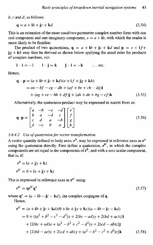
3.6.4.2 Use of quaternion for vector transformation

A vector quantity defined in body axes, rb, may be expressed in reference axes as rn

using the quaternion directly. First define a quaternion, rb , in which the complexcomponents are set equal to the components of rb, and with a zero scalar component,that is, if:

This is expressed in reference axes as r11' using:

i*' = qrb'q* (3.57)

where q* = (a — ib — }c — kJ), the complex conjugate of q.Hence,

(3.58)

Alternatively, rn' may be expressed in matrix form as follows:

rn' = C'rb'

where

and

(3.59)

which is equivalent to writing:

rn = Crb

Comparison with eqn. (3.34) reveals that C is equivalent to the direction cosinematrix C£.

3.6.4.3 Propagation of quaternion with time

The quaternion, q, propagates in accordance with the following equation:

q = 0.5q-p£b (3.60)

This equation may be expressed in matrix form as a function of the componentsof q and p£b = [0, co£b

T]T as follows:

(3.61)

that is,

(3.62)

Equations of this form may be solved in a strapdown navigation system to keeptrack of the quaternion parameters which define body orientation. The quaternionparameters may then be used to compute an equivalent direction cosine matrix,or used directly to transform the measured specific force vector into the chosenreference frame (see eqn. (3.57)).

3.6.5 Relationships between direction cosines, Euler anglesand quaternions

As shown in the preceding sections, the direction cosines may be expressed in termsof Euler angles or quaternions, viz:

(3.63)

By comparing the elements of the above equations, the quaternion elements may beexpressed directly in terms of Euler angles or direction cosines. Similarly, the Eulerangles may be written in terms of direction cosines or quaternions. Some of theserelationships are summarised in the following sections.

3.6.5.1 Quaternions expressed in terms of direction cosines

For small angular displacements, the quaternion parameters may be derived using thefollowing relationships:

(3.64)

A more comprehensive algorithm for the extraction of quaternion parameters fromthe direction cosines, which takes account of the relative magnitudes of the directioncosine elements, is described by Shepperd [2].

3.6.5.2 Quaternions expressed in terms ofEuler angles

(3.65)

3.6.5.3 Euler angles expressed in terms of direction cosines

The Euler angles may be derived directly from the direction cosines as describedbelow. For conditions where 0 is not equal to 90° the Euler angles can be determinedusing

(3.66)

For situations in which 9 approaches n/2 radians, the equations in 0 and \j/ becomeindeterminate because the numerator and the denominator approach zero simulta-neously. Under such conditions, alternative solutions for 0 and ty are sought basedupon other elements of the direction cosine matrix. This difficulty may be overcomeby using the direction cosine elements en, en , Q2 and C23, which do not appear ineqn. (3.66), to derive the following relationships:

(3.67)

For 0 near -\-n/2\

For 9 near — n/2:

(3.68)

Equations (3.67) and (3.68) provide values for the sum and difference of 0 and \j/under conditions where 0 approaches n/2. Separate solutions for 0 and x/r cannot be

obtained when 0 = +n/2 because both become measures of angle about parallel axes(about the vertical), that is, a degree of rotational freedom is lost. This is equivalent tothe 'gimbal lock' (or nadir) condition which arises with a set of mechanical gimbalswhen the pitch, or inner, gimbal is rotated through 90°.

When 6 approaches H-TT/2, either (f> or \fs may be selected arbitrarily to satisfysome other condition while the unspecified angle is chosen to satisfy eqn. (3.68).To avoid 'jumps' in the values of 0 or ^ between successive calculations when 0 is inthe region of+;r/2, one approach would be to 'freeze' one angle, 0, for instance, at itscurrent value and to calculate ^ in accordance with eqn. (3.68). At the next iteration,\f/ would be frozen and (j> determined using eqn. (3.68). This process of updating (f>or \fr alone at successive iterations would continue until 0 is no longer in the regionof+jr/2.

3.7 Detailed navigation equations

3.7.1 Navigation equations expressed in component form

For a terrestrial navigation system operating in the local geographic reference frame,it has been shown (Section 3.5.3) that the navigation equation may be expressedas follows:

(3.69)

where, v£ represents velocity with respect to the Earth expressed in the localgeographic frame defined by the directions of true north, east and the local vertical,in component form:

Ve=[VN VE VDf (3.70)

fn is the specific force vector as measured by a triad of accelerometers and resolvedinto the local geographic reference frame;

fn = [/N / E / D ] T (3.71)

CO6 is the turn rate of the Earth expressed in the local geographic frame;

«fe = [Q cos L 0 - f t sin L]T (3.72)

(Ogn represents the turn rate of the local geographic frame with respect to theEarth-fixed frame; the transport rate. This quantity may be expressed in terms ofthe rate of change of latitude and longitude as follows:

(o£n = [£ cos L -L -I sin L]T (3.73)

Writing t = VE/(RO + h) cos L and L = V^f(Ro + h) yields:

(3.74)

where RQ is the radius of the Earth and h is the height above the surface of the Earth.

gj1 is the local gravity vector which includes the combined effects of the mass attractionof the Earth (g) and the centripetal acceleration caused by the Earth's rotation (<*>ie x(die x R)- Hence, we may write

(3.75)

The navigation equation may be expressed in component form as follows:

(3.76)

(3.77)

(3.78)

where § and rj represent angular deflections in the direction of the local gravityvector with respect to the local vertical owing to gravity anomalies, as discussed inSection 3.7.4.

Latitude, longitude and height above the surface of the Earth are given by:

(3.79)

(3.80)

(3.81)

It is assumed, in the equations given above, that the Earth is perfectly spherical inshape. Additionally, it is assumed that there is no variation in the Earth's gravitationalfield with changes in the position of the navigation system on the Earth or its heightabove the surface of the Earth.

The modifications which must be applied to the navigation equations in order totake account of the errors introduced by these assumptions and so permit accuratenavigation over the surface of the Earth are summarised briefly in the followingsections. The reader requiring a more detailed analysis of these effects is referred tothe texts by Britting [3] and Steiler and Winter [4] in which such aspects are discussedin detail.

3.7.2 The shape of the Earth

It is clear from the preceding analysis that, in order to determine position on the Earthusing inertial measurements, it is necessary to make some assumptions regarding theshape of the Earth. The spherical model assumed so far is not sufficiently represen-tative for very accurate navigation. Owing to the slight flattening of the Earth at thepoles, it is customary to model the Earth as a reference ellipsoid which approximatesmore closely to the true geometry. Terrestrial navigation involves the determinationof velocity and position relative to a navigational grid which is based on the referenceellipsoid; see illustration in Figure 3.21.

In accordance with this model, the following parameters may be defined:

the length of the semi-major axis, R

the length of the semi-minor axis, r = R(I — / )

the flattening of the ellipsoid, / = (R - r)/R

the major eccentricity of the ellipsoid, e = [/(2 — f)]1^2

By modelling the Earth in accordance with a reference ellipsoid as defined here,a meridian radius of curvature (R^) and a transverse radius of curvature (RE) maybe derived in accordance with the following equations:

(3.83)

(3.84)

Polaraxis

Localmeridian

plane

Referenceellipsoid

Surfaceof the earth

(not to scale)

Figure 3.21 Reference ellipsoid

The rates of change of latitude and longitude may then be expressed in terms ofa R^ and R^ as follows:

(3.85)

(3.86)

The mean radius of curvature used in the earlier equations, Ro = (RERN)1^2- Theflattening of the Earth at the poles gives rise to a difference of approximately 20 kmbetween the mean radius used for a spherical earth model and the measured polarradius of approximately 20 km.

Similarly, the transport rate now takes the following form:

(3.87)

Further discussion regarding the shape of the Earth and the choice of datum referenceframes appears in the following section.

With the aid of Figure 3.22, the distinction is drawn here between geocentric andgeodetic latitude (see following section).

Geocentric latitude at a point on the surface of the Earth is the angle between theequatorial plane and a line passing through centre of Earth and the surface locationpoint. Geodetic latitude at a point on the surface of the Earth is the angle betweenthe equatorial plane and a line normal to the reference ellipsoid which passes throughthe point.

North

Geocentriclatitude Geodetic

latitude

Figure 3.22 Geocentric and geodetic latitude

3.7.3 Datum reference models

The surface of the Earth is highly irregular in shape and can be modelled in variousways.

Topographic models represent the physical shape of the Earth and the mean level ofthe oceans.

Geodetic models yield a surface which is perpendicular to the local gravity vectorat all points; an 'equipotential surface'. The resulting shape is referred to as ageoid.

Geodesy is the name given to the study of the size and shape of the Earth, andthe term geodetic navigation is used here to refer to navigation which takes properaccount of this shape. Aspects of geodesy and the use of geodetic datum points formapping, surveying and navigation are discussed in the following paragraphs. For amore detailed discussion of the subject and a full definition of the terminology, thereader is referred to the standard text book by Bomford [5].

Local variations in gravity, caused by variations in the Earth's core and surfacematerials, cause the surface of the geoid, the gravity surface, to be irregular. Whilst it ismuch smoother than the physical surface of the Earth, as represented by a topographicmodel, it is too irregular to be used as a surface in which to specify spatial coordi-nates. For terrestrial navigation, a geometrical shape that approximates closely to thegeoid model is used; an ellipsoid, which in this context is a three-dimensional (3-D)shape formed by rotating an ellipse about its minor axis. The term oblate spheroid issometimes used in place of ellipsoid.

The term geodetic datum is used to define the ellipsoid and its positional relation-ship with respect to the solid Earth. In combination with an axis definition, a geodeticdatum defines a 3-D geographic co-ordinate system, the dimensions being geode-tic latitude and longitude and ellipsoidal height (height above the surface of theellipsoid).

In practice, vertical position is not defined with respect to the surface of theellipsoid because this surface offers no physical reference point for measurement.The geoid, which corresponds approximately to mean sea level, offers a much moreconvenient vertical reference. For this reason, height above mean sea level is mostcommonly used. For land based surveys [6], the reference level used as a zero datumis defined by mean sea level at a selected coastal location, or an average value of meansea level at several locations, over a specified period of time. Land surveys shouldreference the vertical datum chosen. In the United Kingdom, the vertical datum usedis Ordnance Datum Newlyn (ODN) and in the United States, the North AmericanVertical Datum of 1988 (NAVD88).

It is possible to define a geodetic datum which approximates to the shape ofthe Earth over the entire globe. The figures given in Figure 3.23 were defined forsuch a datum by the World Geodetic System Committee in 1984, the WGS-84model [7]. The value of Earth's rate is discussed in Figure 3.24.

Many geodetic datum points used for mapping, surveying and navigation aredefined to provide a more precise fit over a restricted geographical area, the

Figure3.23 WGS-84 model4

The duration of a solar day is 24h, the time taken between successive rotations foran Earth-fixed object to point directly at the sun. The Sidereal day represents thetime taken for the Earth to rotate to the same orientation in space and is of slightlyshorter duration than the solar day, 23h, 56min, 4.1s. The Earth rotatesthrough one geometric revolution each Sidereal day, not in 24h, which accountsfor the slightly strange value of Earth's rate.

Solar day =24hSidereal day = 23 h 56min 4.1 sEarth's day = 1 revolution/Sidereal day

= 7.292115x10"5rad/s= 15.041067%

Earth

Siderealday

Solar day

Figure 3.24 The solar day and the sidereal day

UK Ordnance Survey (OSGB 1936), the British National Grid for example. Regionaldatum points such as this have proliferated over time with the result that their areasof application may overlap. As a consequence, it is necessary when referring to apositional location on the Earth in terms of its latitude and longitude, to specify also

4 The former Soviet Union devised a similar model, SGS-90 or PZ-90, discussed in Appendix D.

Length of the semi-major axis,

Length of the semi-minor axis,

Flattening of the ellipsoid,

Major eccentricity of

the ellipsoid,

Earth's rate (see Figure 3.24),

Figure 3.26 Standard Mercator projection

the corresponding geodetic datum or geographic co-ordinate reference. Contrary tocommon belief, the coordinates alone do not adequately define a particular location.

Lines of constant latitude and longitude are curved in three dimensions, but may berepresented on a plane by means of a projection. The resulting rectangular co-ordinatesystem on the plane is called a grid. Various projections of the Earth's surface intotwo dimensions have been used, using a geodetic reference ellipsoid as the basis forprojection.

A flat grid system can be obtained by projecting the reference ellipsoid ontoa cylindrical, conical or flat shape as indicated in Figure 3.25. It is noted that the JCand y axes must be orthomorphic, that is, of equal scale.

The Standard Mercator projection, illustrated in Figure 3.26, is generated byplacing a cylinder over the Earth so that the contact point is around the equator. A point

Cylindrical

Zenithal Conical

Figure 3.25 Examples of orthomorphic projection schemes used for mapping

Figure 3.28 Universal Transverse Mercatorprojection

on the Earth is projected onto the inside of the cylinder by taking a line from the centreof the Earth through the point (e.g. x to x\ y to / as shown in Figure 3.26). When allpoints have been projected onto the cylinder, the cylinder is unwrapped and laid flat.This type of projection produces the most commonly observed map of the world.

The Mercator is a useful projection for navigation because a bearing directionon the globe is very similar to a direction on the projection. However, distancesand areas will be distorted on small scale maps. Mercator and other projections donot preserve scale or area. For instance, with Standard Mercator, distance along theequator is represented exactly, but distance at higher latitude is magnified. As a result,Greenland appears to be the same size as South America, whereas it is actually aboutone-third of the size.

Various projection techniques are used to overcome the effects of distortion inregional maps where it is required to have a map or rectangular grid system that isappropriate to the locality of interest. For example, the Lambert conical projection,illustrated in Figure 3.27, provides an accurate representation of the area around thepoint of contact between the cone and the reference ellipsoid. Alternatively, the useof a cylinder or cone that cuts the reference ellipsoid in two places close to the area ofinterest may be used. This allows a reduction in the distortion to be achieved adjacentto and between the points of contact, providing two horizontal parallels and minimumvertical distortion.

One of the most commonly used projections is the Universal Transverse Mercator(UTM) projection. This uses the same principle as the Standard Mercator, withthe exception that the cylinder is rotated through 90° so that the contact point ofthe cylinder with the Earth is along a meridian line; see Figure 3.28. To minimise dis-tortion and preserve accuracy, the technique is employed of using only a small strip oneither side of a designated central meridian. The UTM projection is used worldwide.

Figure 3.27 Lambert conical projection

Central meridian

Figure 3.29 Universal Transverse Mercator grid zone

The UTM system uses the Transverse Mercator in separate zones each 6° wide.UTM zones are identified alphanumerically; numbering from 1 to 60, starting with1 in the 1800W-174°W zone and increasing eastwards to 60 in the 174°E-180°Ezone. Hence grid zone 32 is from 6° to 12° longitude. The UTM grid is furthersubdivided into blocks of 8° of latitude from —80° to +80° which are identified bythe use of the letters C to X, excluding I and O (e.g. 64°S-56°S is E).

Any UTM grid zone can be represented as shown in Figure 3.29 where the centralmeridian is an odd number and a multiple of 3. The grid north and the true north willonly be coincident along the central meridian and on the equator. At all other pointsthere is a difference referred to as 'convergence'. It is noted that to the true north iswest of grid north to the right of the central meridian and true north is east of gridnorth to the left of the central meridian.

3.7.4 Variation of gravitational attraction over the Earth

As described earlier, accelerometers provide measurements of the difference betweenthe acceleration with respect to inertial space and the gravitational attraction actingat the location of the navigation system. In order to extract the precise estimates oftrue acceleration needed for very accurate navigation in the vicinity of the Earth,it is necessary to model accurately the Earth's gravitational field. This of course isalso true for navigation close to any other body with a gravitational field.

Grid northWest of central

meridian - grid

convergence is

negative

True north

Grid north

East of central

meridian - grid

convergence is

positive

Northern hemisphere

Equator

Southern hemisphere

Geographic (geodetic)latitude

Figure 3.30 Deflection of local vertical owing to gravity anomalies

It is assumed in the earlier derivation of the navigation equation that the gravityvector acts vertically downwards, that is, normal to the referenced ellipsoid. In prac-tice, both the magnitude and the direction of the gravity vector vary with positionon the Earth's surface and height above it. Variations occur because of the variationbetween the mass attraction of the Earth and gravity vector; the centrifugal accelera-tion being a function of latitude. In addition, gravity varies with position on the Earthbecause of the inhomogenous mass distribution of the Earth. Such deviations in themagnitude and direction of the gravity vector from the calculated values are knownas gravity anomalies.

Mathematical representations of the Earth's gravitational field are discussed insome depth by Britting [3]. The deflection of the local gravity vector from the verticalmay be expressed as angular deviations about the north and east axes of the localgeographic frame as follows:

S = [&, -rig, gf (3.88)

where £ is the meridian deflection and r\ is the deflection perpendicular to the meridian.The deflection in the meridian plane is illustrated in Figure 3.30.

The resulting deviation of the vertical over the surface of the Earth varies by upto 30 arc s.

The precise knowledge of the gravity vector becomes important for certainhigh accuracy applications, such as for marine navigation where the deflection ofthe vertical becomes an important factor. Exact knowledge of the magnitude ofgravity is also vital for the testing of very precise accelerometers, that is, sensorshaving a measurement bias of less than 10~~5g. Similarly, it is important for survey-ing and gravity gradiometry, where attempts are made to measure the gravity vectorvery accurately.

Various international models for the variation of gravity with latitude are given inthe literature. Steiler and Winter [4] give the following expressions for the variation

Polaraxis

Localmeridian

plane

Referenceellipsoid

of the magnitude of the gravity vector with latitude at sea level (h = 0) and its rateof change with height above ground:

S(O) = 9.780318(1+ 5.3024 x 10"3 sin2 L - 5.9 x 10"6sin22L)m/s2

(3.89)

dje(O) , 9 9

-51-1 = -0.0000030877(1 - 1.39 x 10~3 sin2 L) m/s2/m (3.90)dh

For many applications, precise knowledge of gravity is not required and it is sufficientto assume that the variation of gravity with altitude is as follows:

*»-(HS5F <391)

where g(0) is derived from eqn. (3.89).

References

1 WRAY, G.L., and FLYTMN, DJ.: 'An assessment of various solutions of thenavigation equation for a strapdown inertial system'. Technical report 79017, RoyalAircraft Establishment, January 1979

2 SHEPPERD, S.W.: 'Quaternion from rotation matrix', AIAA Journal of Guidanceand Control 1978,1(3)

3 BRITTING, K.: 'Inertial navigation system analysis' (Wiley Interscience,New York, 1971)

4 STEILER, B., and WINTER, H.: 'AGARD flight test instrumentation volume 15on gyroscopic instruments and their application to flight testing'. AGARD-AG-160-VOL.15, September 1982

5 BOMFORD, G.: 'Geodesy' (Oxford University Press Inc., New York City, 1985,4th edn.)

6 WILLIAMSON, H.S., and WILSON, H.F.: 'Directional drilling and earth curva-ture', SPE Drill & Completions, 2000,15 (1)

7 'Department of Defence World Geodetic System 1984: Its definition andrelationship with local geodetic systems'. DMATR 8350.2, September 1987