Basic Production Engineering and Well Performance

Dr. Hemanta MukherjeeiPoint LLCWestminster, CO. 80031January 2011

Texts and References1. Brown, K.E. et al.: “The Technology of Artificial Lift Methods”,“Production Optimization of Oil and Gas Wells by Nodal Systems Analysis,”PennWell Publishing Co., Tulsa, OK (1984), Vol. 4.2. Brown, K.E. et al.: “The Technology of Artificial Lift Methods”,“Introduction of Artificial Lift Systems, Beam Pumping Design and Analysis,Gas Lift”, The Petroleum Publishing Co., Tulsa, OK (1980) Vol. 2a.3. Golan, Michael and Whitson, Curtis H.: Well Performance, PrenticeHall, Englewood Cliffs, NJ (1991).4. Muskat, M.: “The Flow of Homogeneous Fluids Through Porous Media,”The Society of Petroleum Engineers, Inc., 1982, copyright by IHRDC, Boston.5. James P. Brill and Hemanta Mukherjee : Multiphase Flow In Wells, SPEMonograph Volume 17, SPE Dallas, TX (1977) 5.

Drilling Rig

Well Performance Analysis

Also called Production System Analysis

Essential for optimized production from wells

Essential Component of Reservoir Management

Reservoir Management Reservoir Definition/Characterization

Geology / GeophysicsSurface Seismics

Reservoir PerformanceExploratory and Development WellsWell Data - logs,cores,well tests,VSPs etcWell Performance and Issues:

Optimum CompletionWell Surveillance

• Stimulation,Artificial Lift,Pressure Maintenance• Secondary and Tertiary Recovery etc

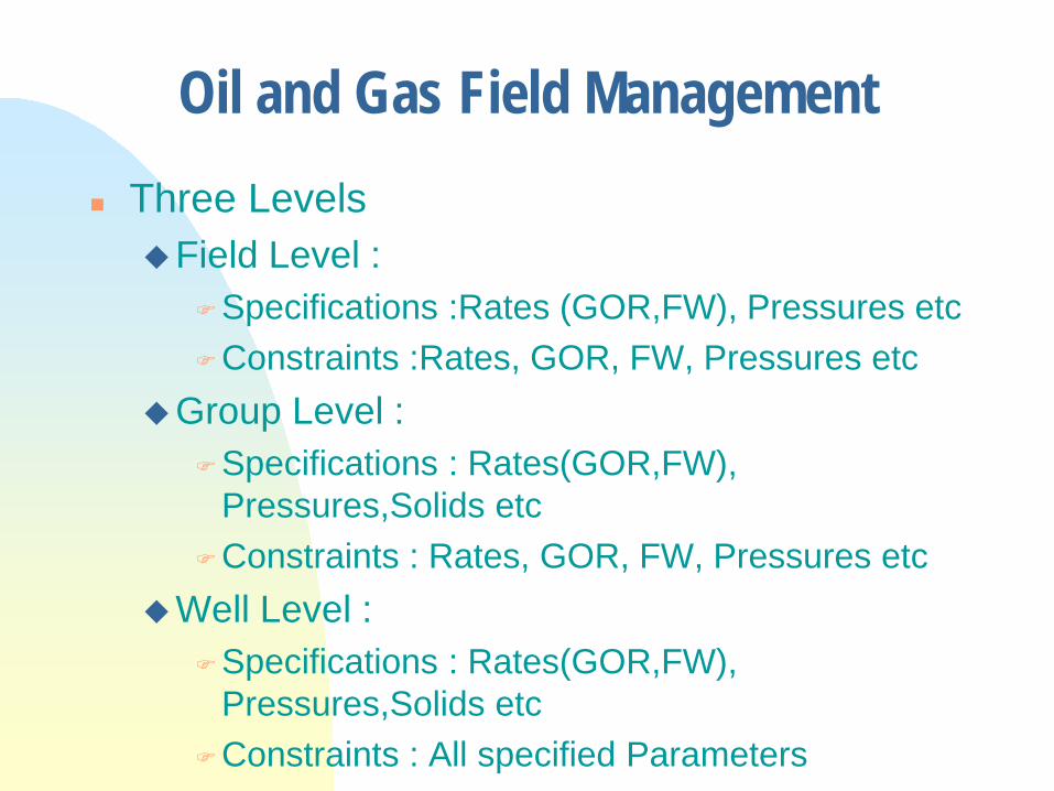
Oil and Gas Field Management Three Levels

Field Level :Specifications :Rates (GOR,FW), Pressures etcConstraints :Rates, GOR, FW, Pressures etc

Group Level :Specifications : Rates(GOR,FW),

Pressures,Solids etcConstraints : Rates, GOR, FW, Pressures etc

Well Level :Specifications : Rates(GOR,FW),

Pressures,Solids etcConstraints : All specified Parameters

Why Manage Reservoirs ?

Earnings and Investment AppraisalRevenue Projections --- Oil & Gas Price

Investment Decisions Based on Revenue Overall Development Strategy

Primary Recovery / Artificial LiftSecondary RecoveryTertiary RecoveryPossible Environmental Impact

Engineering Tools Used

Formation Evaluation - Geological Information , Rock and

Fluid Properties

Reservoir SimulatorPredictionHistory Matching

Well Performance and Completion SimulatorsManagement of a Reservoir at the Well Level

Historical Preview

W.E.Gilbert ( 1944,1954 ) of ShellFlowing and Gas Lift Well Performance (Concept)

ProblemsComputersLack of understanding of MultiPhase Flow in Pipes

and Piping ComponentsPoettman and Carpenter ( 1952 ) - Oil & Gas Flow

in Vertical Pipes

Historical Preview ( Contd. )

A. E. Dukler( 1969 ) Revolution in Computer Technology ( 1960s ) H.D.Beggs and J.P.Brill ( 1973 ) - Gas-Liquid

Flow in Inclined Pipes Joe Mach, E.A. Proano and Kermit Brown (1977)

Systems Analysis

Objectives and Importance

Optimization of Oil & Gas Well Performance Minimization of unnecessary Well Costs

Optimum Tubing sizeOptimum Separator PressureOptimum Completion

Perforation : Shot Density, Tunnel Length, Phasing etc

Stimulation • Fracturing : Half Length, Conductivity• Matrix Treatments : Acid, Solvents, Scale Removal etc

Objectives and Importance (Contd.)

Optimization of Artificial Lift Prediction and Control of Unacceptable

Production ConditionsSlugging or Surging

Slug CatchersVelocity strings

Liquid LoadingVelocity Strings, Plunger Lift

Control of Undesired - Water and Gas

Economic Impact

Maximization of Return on Investment ( ROI ) Net Present Value ( NPV ) Considerations

8

76

5

4

3 2 1

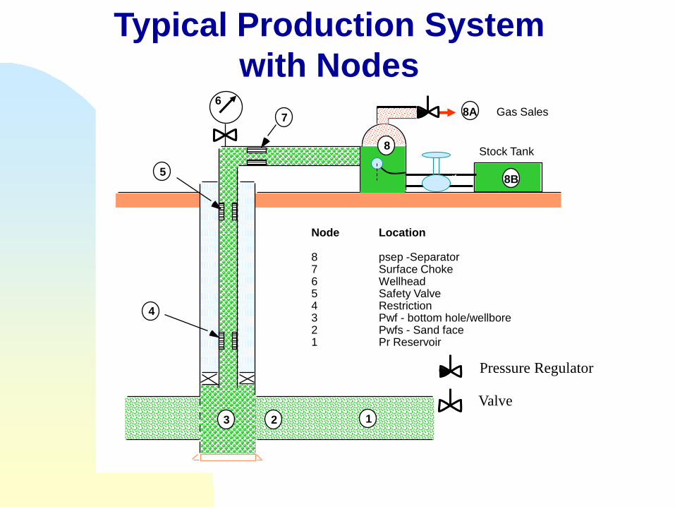
Node Location

8 psep -Separator7 Surface Choke6 Wellhead5 Safety Valve4 Restriction3 Pwf - bottom hole/wellbore2 Pwfs - Sand face1 Pr Reservoir

8A

8B

Gas Sales

Stock Tank

Pressure Regulator

Valve

Typical Production System with Nodes

What is a Node?

Any point in the well Rate into the node = Rate out

of the node Only one pressure exists at

the node

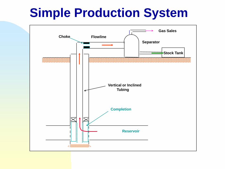
Simple Production System

Vertical or InclinedTubing

Choke FlowlineGas Sales

Separator

Stock Tank

Reservoir

Completion

Possible Pressure Losses in Production System

PwhGas Sales

Separator

Stock Tank

∆P1 = (Pr - Pwfs) = Loss in Porus Medium∆P2 = (Pwfs - Pwf) = Loss across Completion∆P3 = (PUR - PDR) = Loss across Restriction∆P4 = (PUSV - PDSV) = Loss across Safety Valve∆P5 = (Pwh - PDSC) = Loss across Surface Choke∆P6 = (PDSC - Psep) = Loss in Flowline∆P7 = (Pwf - Pwh) = Total Loss in Tubing∆ P8 = (Pwh - Psep) = Total Loss in Flowline

∆P5

∆P8

∆P6

PUR

PDR∆P3

∆P1

PDSV

PUSV

∆P4

∆P7

Pr∆P2Pwf Pwfs

Psep

Pressure Balance

( )p p p p p p pwf sep h fl t ch f acc= + + + + +∆ ∆ ∆ ∆ ∆

Subscripts:

sep = Separator

h = Hydrostatic

fl = Flow Line

t = Tubing

acc = Acceleration

Tubing gradients

9,810 ft at top perf.

0

2000

4000

6000

8000

10000

12000

0 500 1000 1500 2000 2500 3000 3500Pressure (psig)

<--

---

Dep

th (

ft)

Ansari

Aziz

BB

HB

Muk BR

ORK

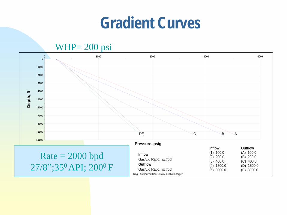
Gradient Curves

0 1000 2000 3000 40000

1000

2000

3000

4000

5000

6000

7000

8000

9000

10000Pressure, psig

Dep

th, f

t

Gradient (A) Case 2 (B)

Case 3 (C) Case 4 (D)

Case 5 (E) Not Used

ABCDE

Inflow

Outflow

Inflow Outflow

Gas/Liq Ratio, scf/bbl

Gas/Liq Ratio, scf/bbl

(1) 100.0 (A) 100.0(2) 200.0 (B) 200.0(3) 400.0 (C) 400.0(4) 1500.0 (D) 1500.0(5) 3000.0 (E) 3000.0

Reg: Authorized User - Dowell Schlumberger

WHP= 200 psi

Rate = 2000 bpd27/8”;350 API; 2000 F

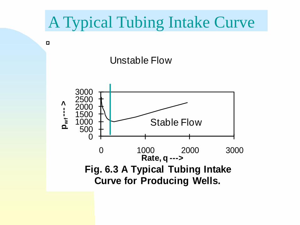
0500

10001500200025003000

0 1000 2000 3000

p wf-

-->

Rate, q --->Fig. 6.3 A Typical Tubing Intake

Curve for Producing Wells.

Stable Flow

Unstable Flow

A Typical Tubing Intake Curve

qg = gas rate, Mscf/Dre = reservoir radius, ft

qo = oil rate, bopdre = reservoir radius, ft

Units

( )q kh

p p

Brr

So

r wf

o oe

w

= ×−

− +

−7 08 1034

3.

lnµ

PI qp p

kh

B rr

Sr wfo o

e

w

=−

= ×

− +

−7 08 10

34

3.

lnµ

Darcy’s Law (Liquid): PSS

Skin Effect

ST = Sdrill + Scement + Sperfs+Sgp+Dq + S(time) + Spseudo+etc

Sdrill = Sinv + Drilling Induced Skin

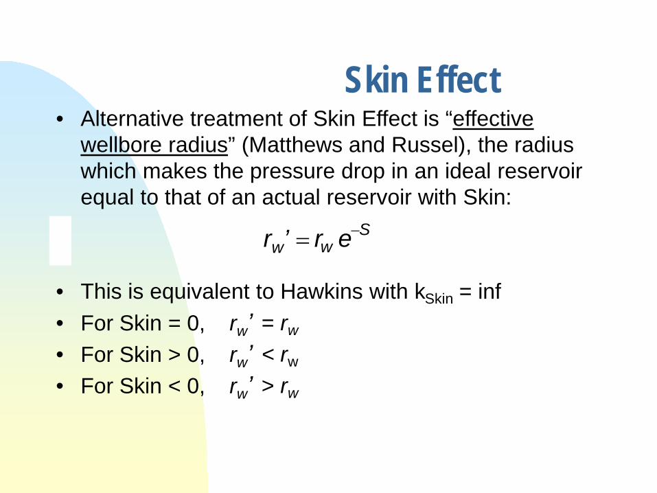
• Alternative treatment of Skin Effect is “effectivewellbore radius” (Matthews and Russel), the radiuswhich makes the pressure drop in an ideal reservoirequal to that of an actual reservoir with Skin:

••• This is equivalent to Hawkins with kSkin = inf• For Skin = 0, rw’ = rw

• For Skin > 0, rw’ < rw

• For Skin < 0, rw’ > rw

Sw errw’ −=

Skin Effect

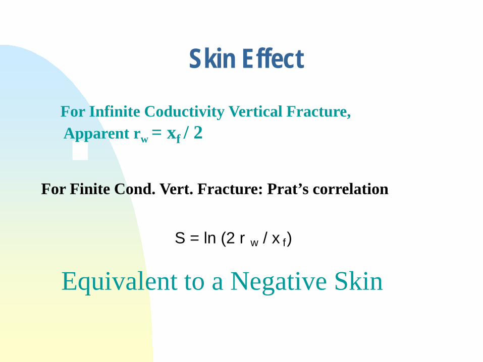
S = ln (2 r w / x f)

For Finite Cond. Vert. Fracture: Prat’s correlation

Skin Effect

For Infinite Coductivity Vertical Fracture,Apparent rw = xf / 2

Equivalent to a Negative Skin

• Added pressure difference due to Skin effect• k around well can be damaged by well drilling

process, by frac, acid or perfs. To accommodate forthis, Van Everdingen defined and area of infinitesimalsize around the wellbore

• For (+) Skin - OK• For (-) Skin - difficult physical interpretation• Hawkins defined Skin of finite radius rSkin with kSkin:

w

Skin

Skin rr

kkS ln)( 1−=

• Unfortunately, there is no unique rSkin, kSkin for any S

Skin Effect

Rate, q (STB/D)

Darcy’s Law (Liquid)

AOFP

pr

Inflow Performance Relationship (IPR)

Rate, q (STBO/D)

Darcy’s Law (Liquid)

AOFP = 3,672 STBO/D

3,000

J = 1.22 STBO/psi-D

Productivity Index (J)

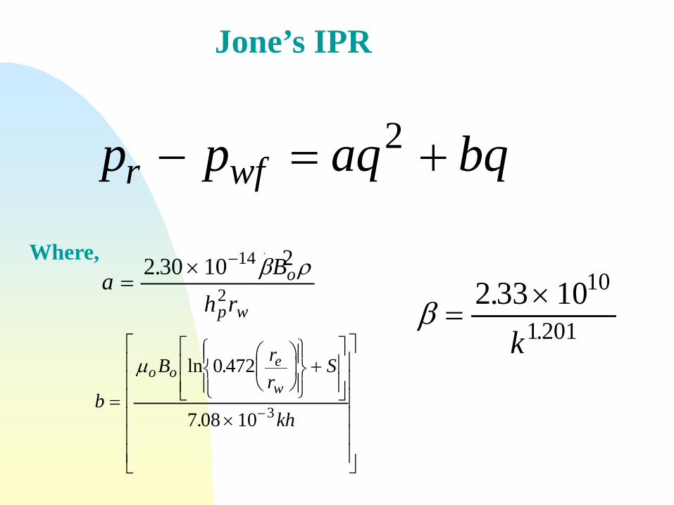
p p aq bqr wf− = +2

Jone’s IPR

,

a Bh r

o

p w=

× −2 30 10 14

2. β ρ

β =×2 33 1010

1 201.

.k

b

B rr

S

kh

o oe

w=

+

×

−

µ ln .

.

0 472

7 08 10 3

Where, 2

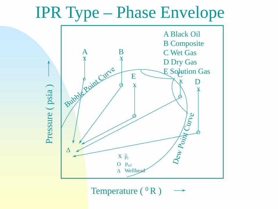
Temperature ( 0 R )

Pres

sure

( ps

ia )

A B

E CD

A Black OilB CompositeC Wet GasD Dry GasE Solution Gas

X X

XX

X

οΟ

Ο

Ο

Ο

∆

Ο ∆

X prpwfWellhead

IPR Type – Phase Envelope

q qpp

ppo o

wf

r

wf

r= − −

max . .1 0 2 08

2

Vogel’s IPR ( Oil Below Bubble Point )

−−=

∗+2

8.02.01)8.1

(b

wf

b

wfbo p

pppbqq

pPI

Vogel’s IPR ( Composite Reservoir )

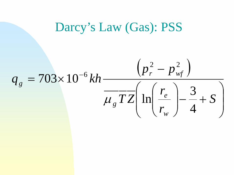
Darcy’s Law (Gas): PSS

( )

+−

−×= −

Srr

ZT

ppkhq

w

eg

wfrg

43ln

1070322

6

µ

( )

+−

−=

Srr

ZT

ppkhq

w

eg

wfrg

43ln

1424

22

µ

Darcy’s Law (Gas)

Jone’s IPR ( Gas )

p p aq bqr wf2 2 2− = +

aTZ

h rg

p w=

× −316 10 12

2

. βγ

b

TZ rr

S

kh

ge

w=

×

+

−1424 10 0 4723. ln .µ

q c p pg r wf

n= −

2 2

c kh

TZ rr

Sge

w

= ×

− +

−703 10

34

6

µ ln

0 5 1. < <n,

Where,

Back Pressure Equation

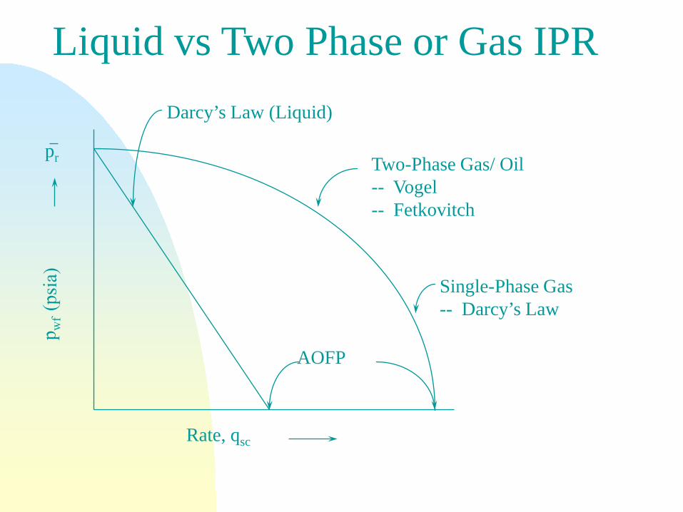
Rate, qsc

Darcy’s Law (Liquid)

Two-Phase Gas/ Oil-- Vogel-- Fetkovitch

Single-Phase Gas-- Darcy’s Law

AOFP

pr

Liquid vs Two Phase or Gas IPR

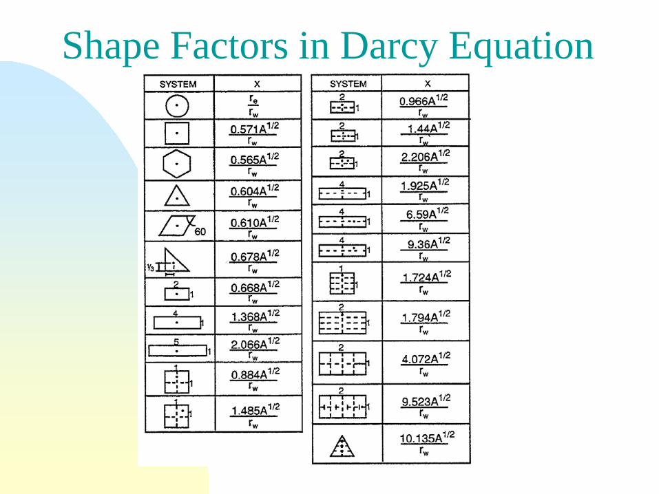
Shape Factors in Darcy Equation

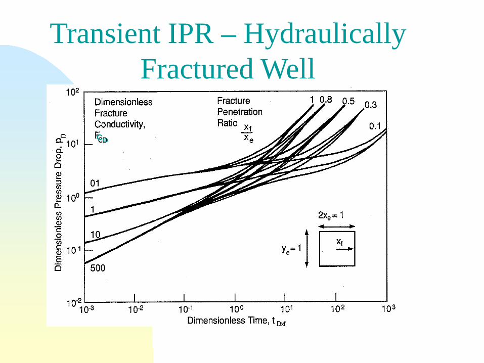
CfD

Transient IPR – Hydraulically Fractured Well

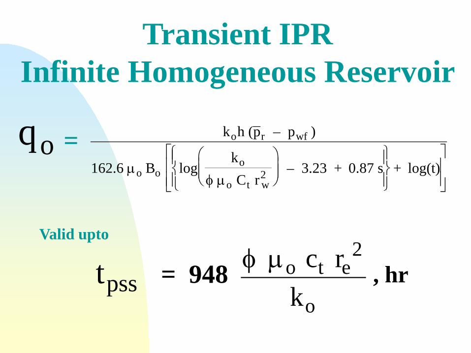
qo k h (p – p )

162.6 B logk

C r – 3.23 + 0.87 s + log(t)

o r wf

o oo

o t w2µ

φ µ

=

Valid upto

tpssφ µo t e

o

c rk

2= 948 , hr

Transient IPRInfinite Homogeneous Reservoir

Transient IPRs

Horizontal Well

Vertical Well Drainage Model

h rev

2rw

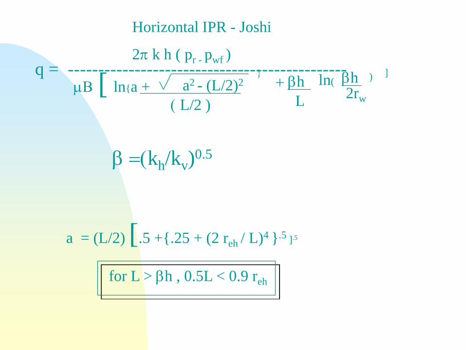
q = ----------------------------------------------2π k h ( pr - pwf )

µΒ [ ln{a + a2 - (L/2)2}

( L/2 )+ βh

Lln( βh

2rw

) ]

β =(kh/kv)0.5

a = (L/2) [.5 +{.25 + (2 reh / L)4 }.5 ].5

for L > βh , 0.5L < 0.9 reh

Horizontal IPR - Joshi

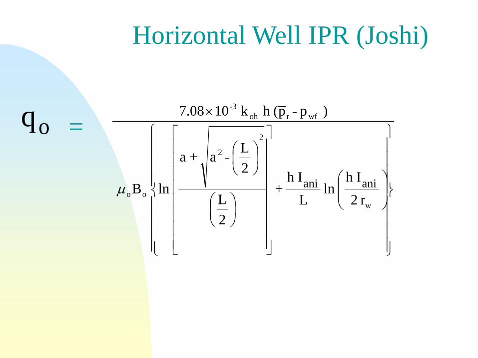
qo

×

w

2

2

oo

wfr oh-3

r 2Ih

ln LIh

+

2L

2L a+a

ln B

) p p(h k 10 7.08

anianiµ

=

Horizontal Well IPR (Joshi)

( )

×≡

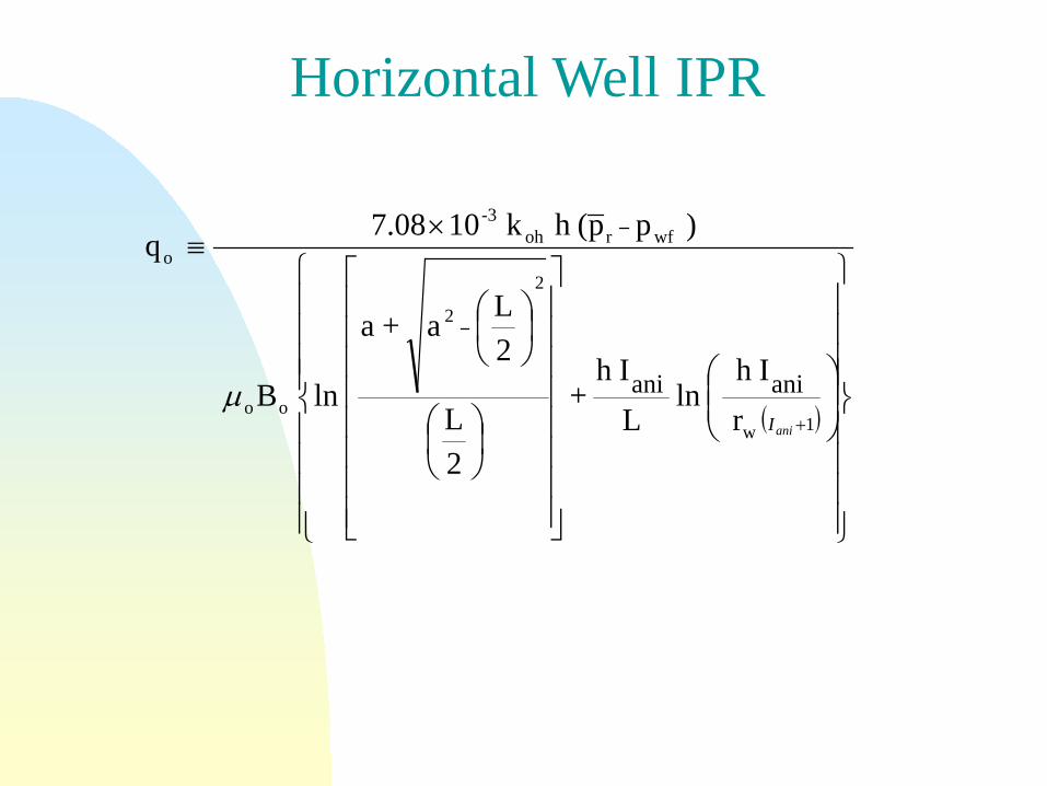
+1w

2

2

oo

wfr oh-3

o

r Ih

ln LIh

+

2L

2L a+a

ln B

) p p(h k 10 7.08 q

anianianiI

µ

Horizontal Well IPR

( )

+−

×≡

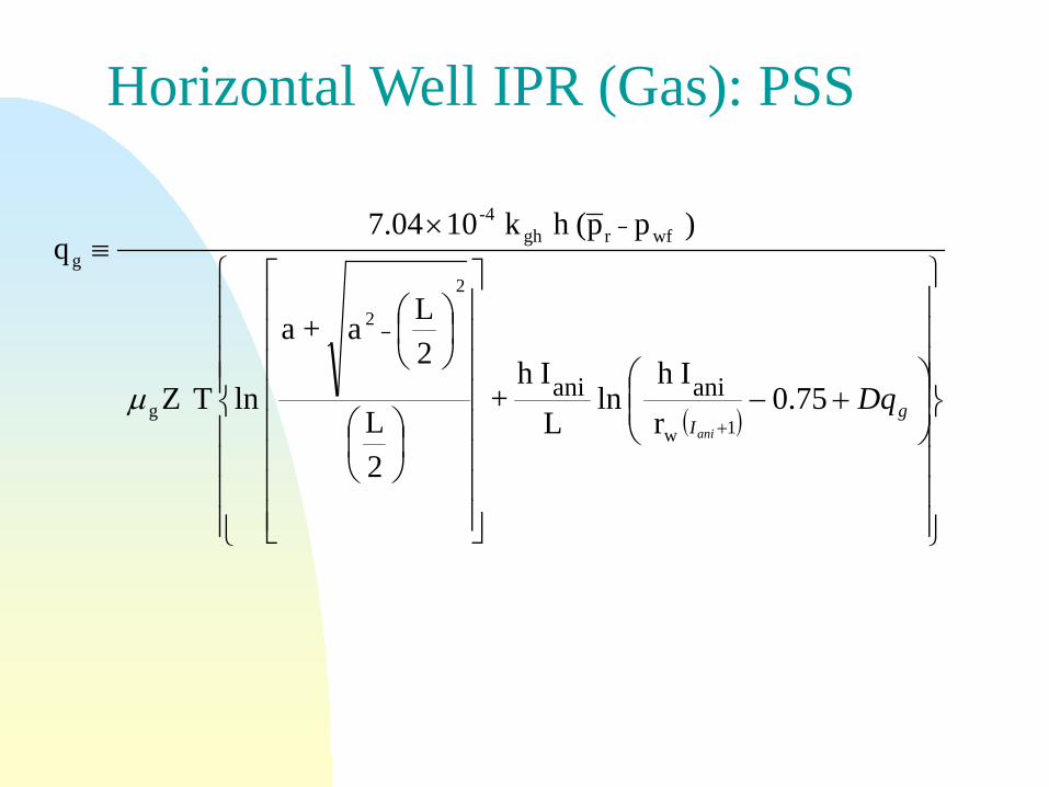
+g

IDq

ani

75.0r

Ih ln

LIh

+

2L

2L a+a

ln TZ

) p p(h k 10 7.04 q

1w

2

2

g

wfr gh-4

g

anianiµ

Horizontal Well IPR (Gas): PSS

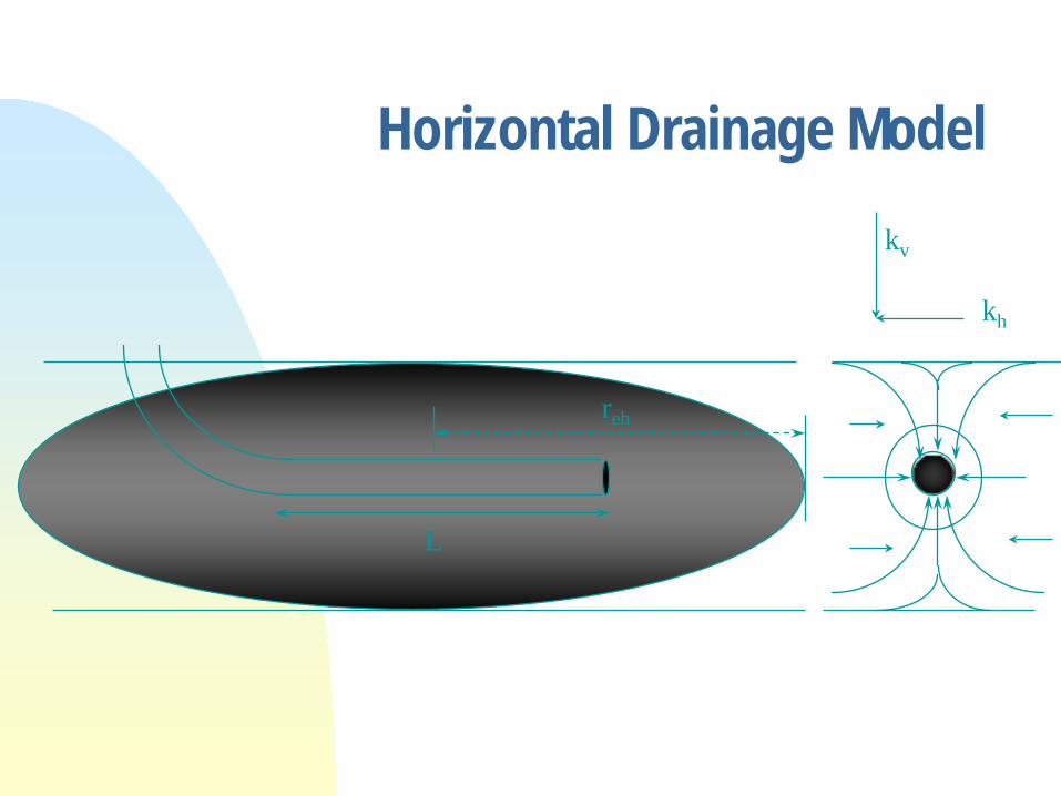
Horizontal Drainage Model

L

reh

kh

kv

Horizontal Well - Flow Components

Β

= +

Β

Α

Α

Α Α

Β

Β2a

h

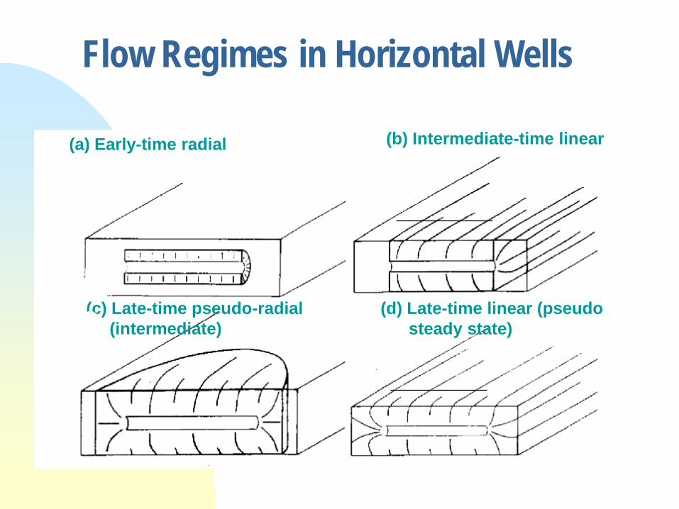
Flow Regimes in Horizontal Wells

(a) Early-time radial (b) Intermediate-time linear

(c) Late-time pseudo-radial(intermediate)

(d) Late-time linear (pseudosteady state)

Goode et alOdeh et al

SPE 69700 : Example of Gull Wing, Crows Feet and Fishbone Multilaterals

Well Performance

A typical systems graph

pwf

( psi )

Rate

pr

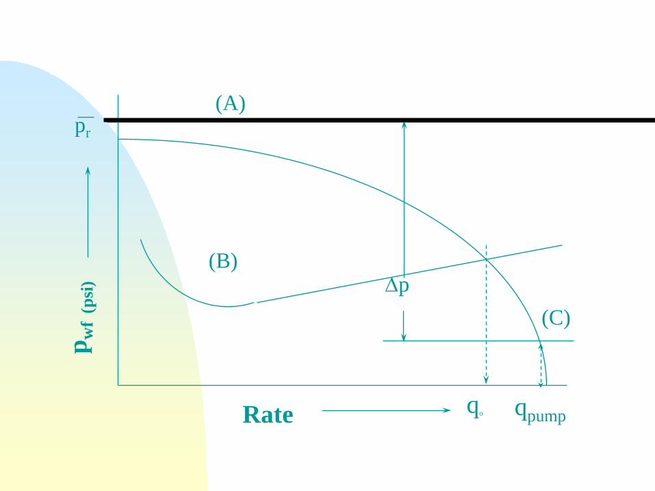
p wf

(psi

)

Rate qo

(A)

(B)

(C)

pr

qpump

∆p

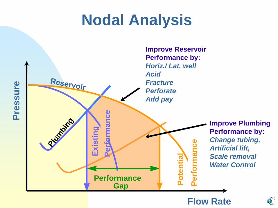
Nodal AnalysisPr

essu

re

Flow Rate

Improve ReservoirPerformance by: Horiz./ Lat. wellAcidFracturePerforateAdd pay

Exis

ting

Perf

orm

ance

PerformanceGap Po

tent

ial

Perf

orm

ance

Improve PlumbingPerformance by:Change tubing,Artificial lift,Scale removalWater Control

Flowrate

- Single well IPR = f (t, Np) - Plumbing - Pwf Caused By Pumps

• Lift System Problems•ESP ( CAMCO )

Potential

Actual

Actual

Potential

Actual

Potential

Actual

Potential

- P = f (q)

P

Services Needed to Define Unknown Reservoir Parameters :

Parameters Affecting Performance :

Remedial Actions / Solutions :

Production GapRESERVOIRPERFORMANCE

COMPLETIONPERFORMANCE

FLOW CONDUITPERFORMANCE

ARTIFICIAL LIFTPERFORMANCE

OBJECTIVE

Bot

tom

Hol

e Fl

owin

g Pr

essu

re

2spf

12 spf

OBJECTIVE OBJECTIVE OBJECTIVE

Flowrate Flowrate Flowrate

Bot

tom

Hol

e Fl

owin

g Pr

essu

re

Bot

tom

Hol

e Fl

owin

g Pr

essu

re

• PVT• Darcy’s Law• Physical Description• Impact

• Perfs• Sand Control• Acid/ Skin• Zone Isolation

• Tubing & Flowlines• Traps• Restrictions• Erosional Velocity

• PTA / RST• PL• DPS

• SPAN / PL• RST• USI

• Calipers / CCL• USI • PL

• PL / Data Pump

• Perforation• Stimulation - Frac/Acid• Squeeze Cem.- Isolation• Laterals

• Reperforate• Gravel Pack• Squeeze Cementing• Acidizing

• Acidizing• Scale Removal (CT)• CT Completion

• Velocity String

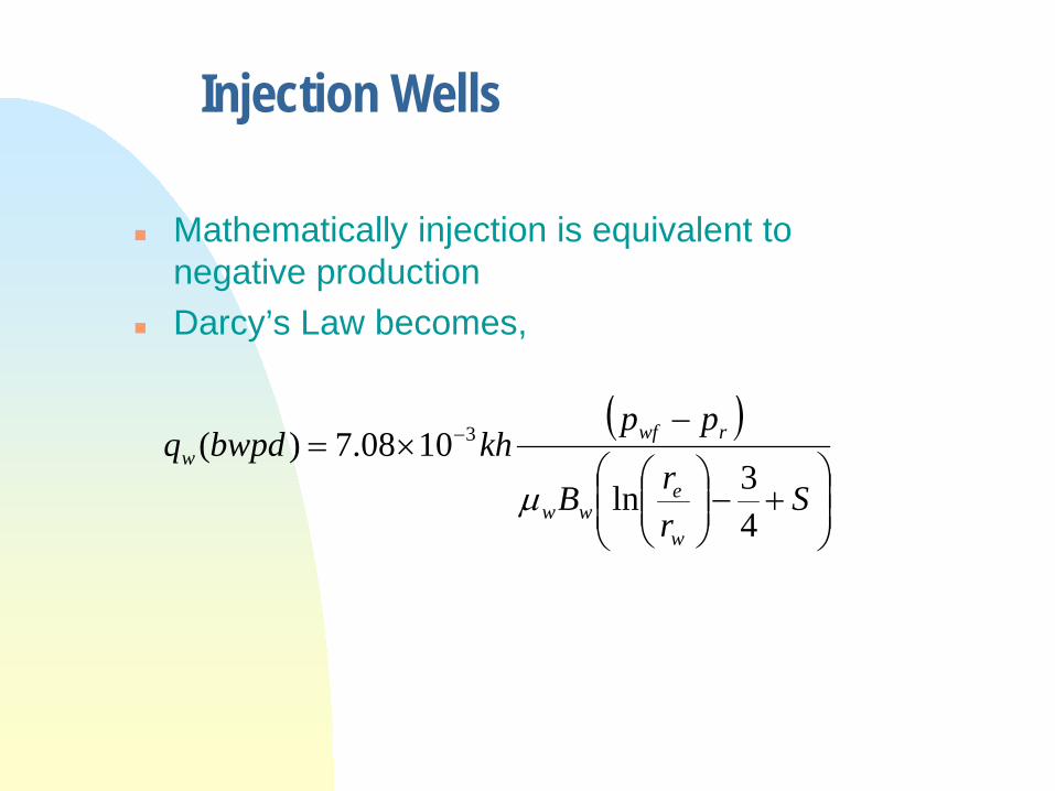
Injection Wells

Mathematically injection is equivalent to negative production

Darcy’s Law becomes,

( )

+−

−×= −

SrrB

ppkhbwpdq

w

eww

rwfw

43ln

1008.7)( 3

µ

Systems Graph- Injection Well

Fracture Pressure

p wi -

-

Injection Rate --

pr

qi

Completion

PerforationMcLeod Model

Gravel PackJones, Blount and Glaze Model

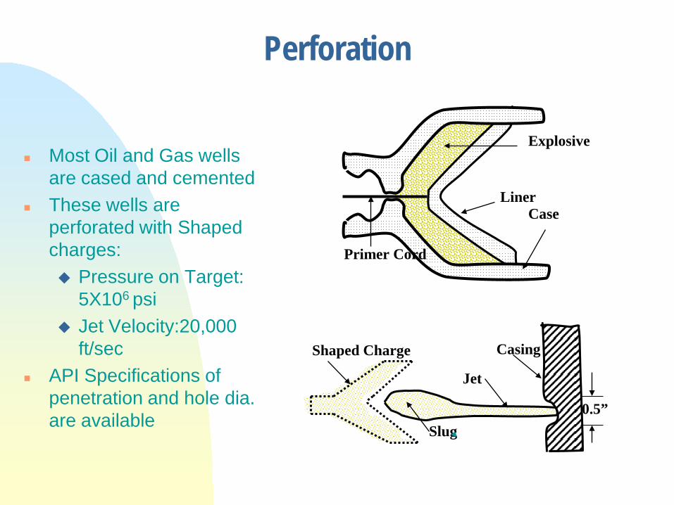
Perforation

Most Oil and Gas wells are cased and cemented

These wells are perforated with Shaped charges: Pressure on Target:

5X106 psi Jet Velocity:20,000

ft/sec API Specifications of

penetration and hole dia. are available

Liner

Explosive

Case

Primer Cord

Shaped Charge

Slug

Jet

0.5”

Casing

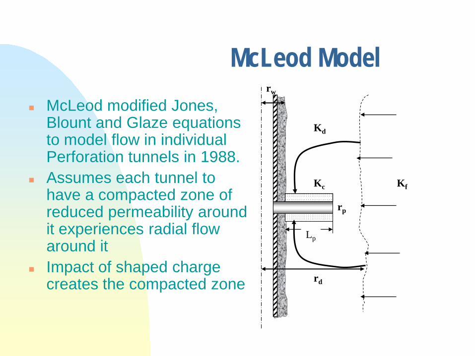
McLeod Model McLeod modified Jones,

Blount and Glaze equations to model flow in individual Perforation tunnels in 1988.

Assumes each tunnel to have a compacted zone of reduced permeability around it experiences radial flow around it

Impact of shaped charge creates the compacted zone

Lp

Kd

KfKc

rp

rd

rw

Perforation Model (oil)

qkL

rrB

qL

rrB

ppp

p

coo

p

cpo

×

+

−×

=∆ −

−

32

2

214

1008.7

ln111030.2 µρβ

pwfs – pwf = aq2 + bq = ∆p

201.1

101033.2

pk×

=β

Perforation Model (gas)

qLk

rrTZ

qL

rrTZ

pp

p

c

p

cpg

×

+

−×

=

− ln10424.1111016.3 3

22

12 µβγ

p2wfs – p2

wf = aq2 + bq

201.1

101033.2k

×=β

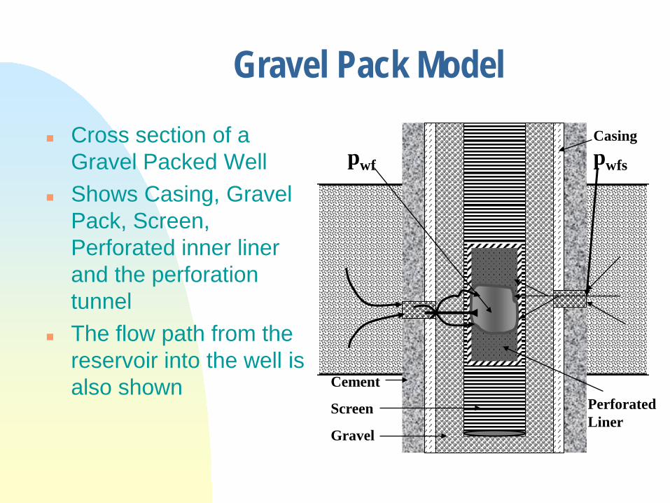
Gravel Pack Model Cross section of a

Gravel Packed Well Shows Casing, Gravel

Pack, Screen, Perforated inner liner and the perforation tunnel

The flow path from the reservoir into the well is also shown

pwf pwfs

Cement

Screen

Gravel

Casing

PerforatedLiner

Gravel Pack Model (oil)

qAk

LBqA

LBpg

oo3

22

213

10127.11008.9

−

−

×+

×=∆

µρβ

pwfs – pwf = aq2 + bq

55.0

71047.1

gk×

=β

Gravel Pack Model (gas)

qAk

TZLqA

TZLpp

g

gwfwfs

µβγ 32

2

1022 1093.810247.1 ×

+×

=−−

p2wfs – p2

wf = aq2 + bq

55.0

71047.1

gk×

=β

Perform Example

Water injection well Vertical well

Dep

th

(ft)

Pressure (psig)

pr

pwhpwh

A

B

Tubing Gradient

0

0

qo

∆p

Casing Gradient

pc

pc

pwf

Gas Lift System

Dep

th (f

t)

Pressure (psig)

prRat

e (S

TBO

/D)

qo

pwh pwh

A

BC

Tubing Gradient

∆ppump

0

0pwf

Pump IntakePressure

Pump DischargePressure

Pumped System

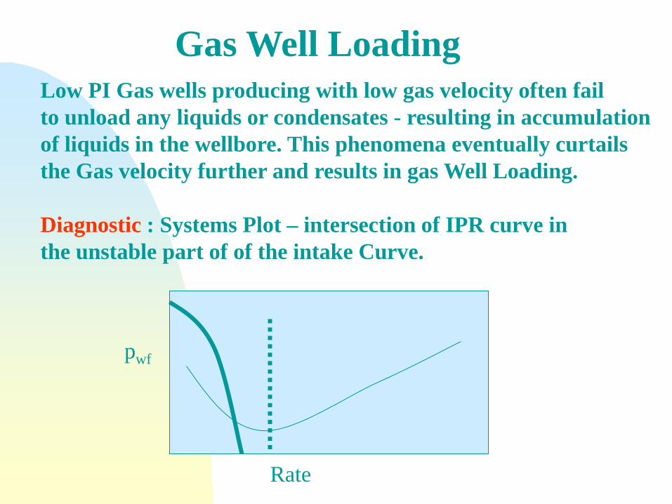
Gas Well LoadingLow PI Gas wells producing with low gas velocity often fail to unload any liquids or condensates - resulting in accumulationof liquids in the wellbore. This phenomena eventually curtailsthe Gas velocity further and results in gas Well Loading.

Diagnostic : Systems Plot – intersection of IPR curve in the unstable part of of the intake Curve.

pwf

Rate

“Gas flow rate at every point in the Tubing has to exceed the critical gasflow rate”

Criteria for Gas WellUnloading

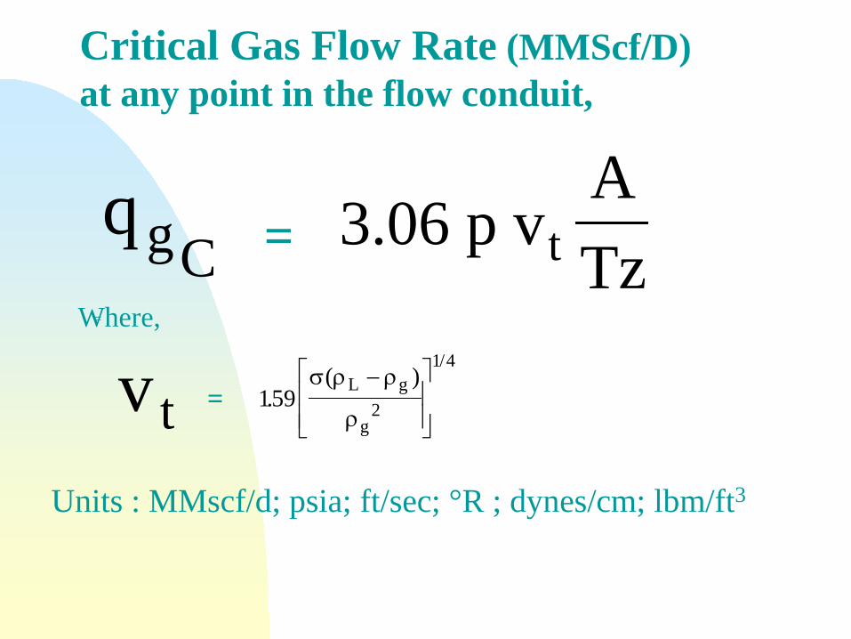
qgC 3.06 p vATzt=

Critical Gas Flow Rate (MMScf/D) at any point in the flow conduit,

Where,=

v t 159 2

1 4

.( )

/σ ρ ρ

ρL g

g

−

=

Units : MMscf/d; psia; ft/sec; °R ; dynes/cm; lbm/ft3

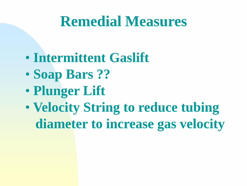
Remedial Measures

• Intermittent Gaslift• Soap Bars ??• Plunger Lift• Velocity String to reduce tubing

diameter to increase gas velocity

Erosion – A real Production Problem

Erosional Velocity

ev C

ρ

=

C = 300 for Liquid impinging on Steel anderosion at 10 mils/year

Units : ft/sec and lbm/ ft3 .

Concept of Equivalent Stagnation Length

Salama and Venkatesh

h = 496920 ( )q v T dsd p2 2/

h = penetration rate in Elbow, mil/yr1 mil = .001 in. or .0254 mmqsd = sand production rate, ft3 / DVp = particle impact velocity, ft/secT = elbow metal hardness, psi (Ref . 37)d = elbow diameter, in

Erosional Velocity - Elbow

v d qe sd= 173. /

Assume:

T = 1.55 e+5 psih = 10 mils/yr

Geothermal and Hydrothermal Gradients in different environments.

Permafrost Marine Environment Earth’s CrustTemperature

Dep

th

Thermal GradientHydrate Zone

Hydrate Formation Temp.

Seabed

Hydrates and Scales

• Clathrate Hydrates – Solids

• Scales

•Organic : Wax and Asphalts

•Inorganic : Sulphates, Chlorides, carbonates

•Mobile Formation Fines

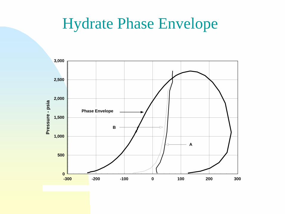
-300 -200 -100 0 100 200 300

Temperature - F

0

500

1,000

1,500

2,000

2,500

3,000

Pres

sure

- ps

ia

Phase Envelope

A

B

Hydrate Phase Envelope

Tubing and Casing patches

Reasons:• To patch holes, corroded or weaker parts• To remediate water or gas leakage• To patch perforations that are water or

gas invaded• provided cement integrity is not a problem

• To isolate zones that are not productive• To protect parts of tubing and casing from

surface damage

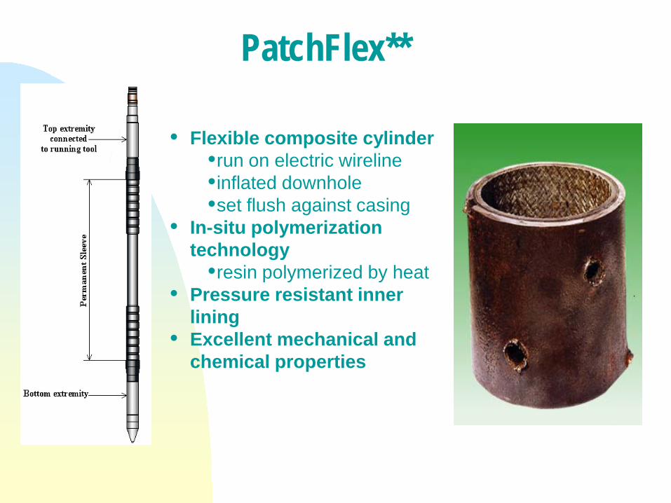
Flexible composite cylinderrun on electric wirelineinflated downholeset flush against casing

In-situ polymerization technologyresin polymerized by heat

Pressure resistant inner lining

Excellent mechanical and chemical properties

PatchFlex**

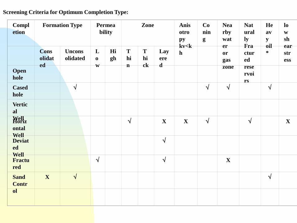
Screening Criteria for Optimum Completion Type:

Completion

Formation Type Permeability

Zone Anisotropykv<kh

Coning

Nearby water or gas zone

Naturally Fractured reservoirs

Heavy oil*

lowshear stress

Consolidated

Unconsolidated

Low

High

Thin

Thick

Layered

Open hole

Cased hole

√ √ √ √

Vertical WellHorizontal Well

√ X X √ √ X

Deviated Well

√

Fractured

√ √ X

Sand Control

X √ √

Texts and References1. Brown, K.E. et al.: “The Technology of Artificial Lift Methods”,“Production Optimization of Oil and Gas Wells by Nodal Systems Analysis,”PennWell Publishing Co., Tulsa, OK (1984), Vol. 4.2. Brown, K.E. et al.: “The Technology of Artificial Lift Methods”,“Introduction of Artificial Lift Systems, Beam Pumping Design and Analysis,Gas Lift”, The Petroleum Publishing Co., Tulsa, OK (1980) Vol. 2a.3. Golan, Michael and Whitson, Curtis H.: Well Performance, PrenticeHall, Englewood Cliffs, NJ (1991).4. Muskat, M.: “The Flow of Homogeneous Fluids Through Porous Media,”The Society of Petroleum Engineers, Inc., 1982, copyright by IHRDC, Boston.5. James P. Brill and Hemanta Mukherjee : Multiphase Flow In Wells, SPEMonograph Volume 17, SPE Dallas, TX (1977) 5.

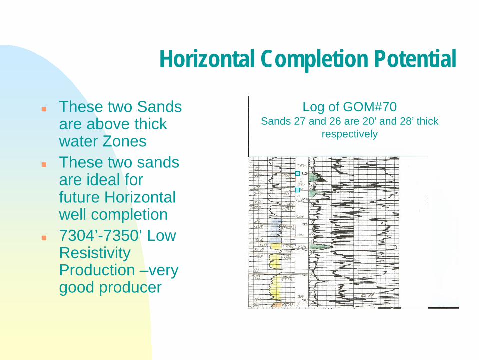
Horizontal Completion Potential

These two Sands are above thick water Zones

These two sands are ideal for future Horizontal well completion

7304’-7350’ Low Resistivity Production –very good producer

Log of GOM#70Sands 27 and 26 are 20’ and 28’ thick

respectively

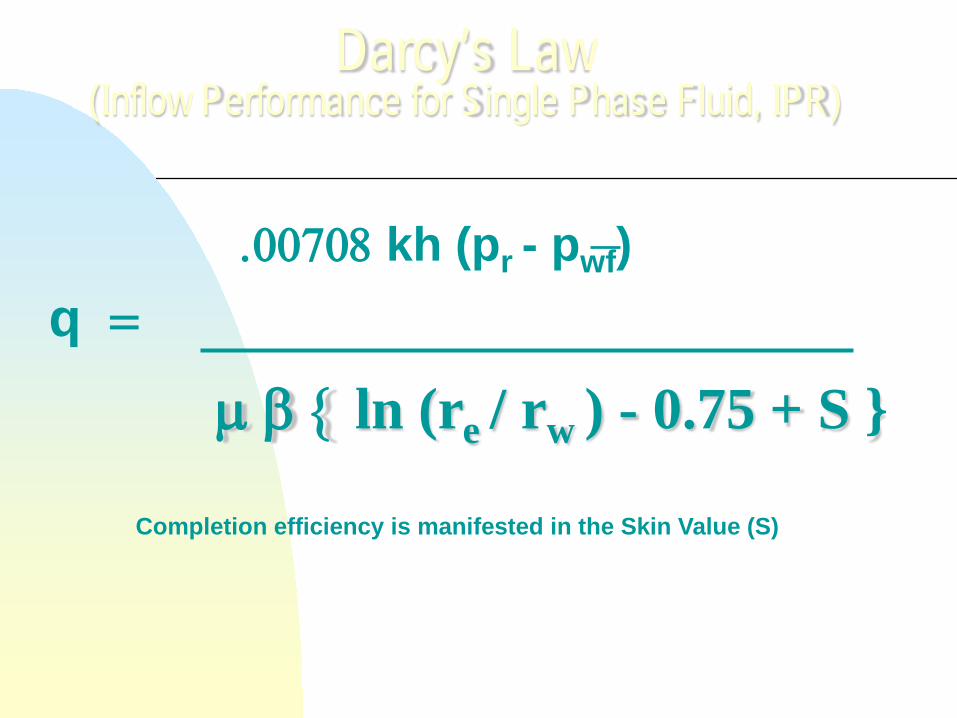
Darcy’s Law(Inflow Performance for Single Phase Fluid, IPR)

.00708 kh (pr - pwf)q =

µ β { ln (re / rw ) - 0.75 + S }

Completion efficiency is manifested in the Skin Value (S)

Horizontal/Lateral Well Screening Criteria

Thin Zones – Difficult to Fracture Effectively High vertical permeability Zones with bottom water Higher Vertical Permeability than Radial Perm.

Naturally Fractured Reservoirs e.g. Rospo Mare field, Italy (Total- Old Elf publications in early1980s)

Drilling Access – Pad Drilling, Island to offshore location etc (Example: Sakhalin Island)

Horizontal Well Applications

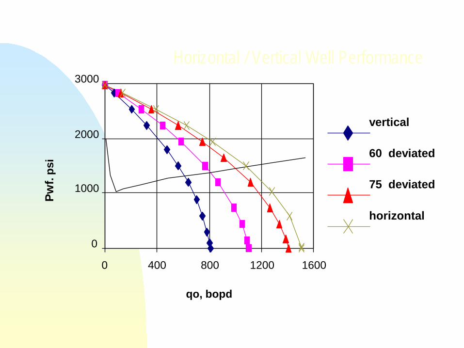
0

1000

2000

3000

0 400 800 1200 1600

qo, bopd

Pwf.

psi

vertical

60 deviated

75 deviated

horizontal

Horizontal / Vertical Well Performance