Basic ranking Models

Boolean and Vector Space Models

Document Processing

Indexing

Ranking

s 3

Boolean Model

Two “classic” models

• Boolean• Vector Space

5

The Boolean Model

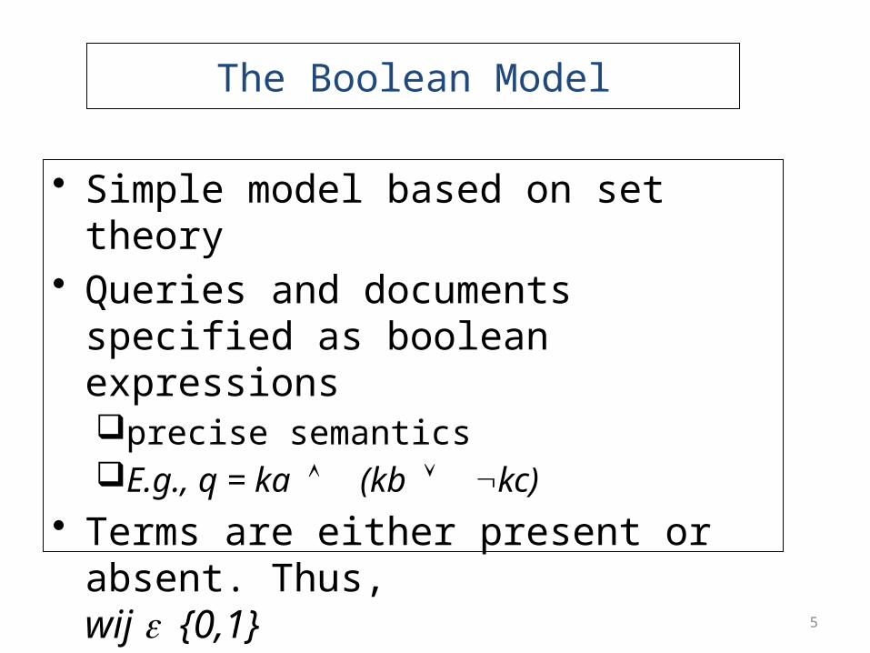
• Simple model based on set theory• Queries and documents specified as

boolean expressions precise semanticsE.g., q = ka (kb kc)

• Terms are either present or absent. Thus, wij {0,1}

6

Example

q = ka (kb kc)vec(qdnf) = (1,1,1) (1,1,0) (1,0,0)

» Disjunctive Normal Form

vec(qcc) = (1,1,0) » Conjunctive component

• Similar/Matching documents• md1 = [ka ka d e] => (1,0,0)• md2 = [ka kb kc] => (1,1,1)

• Unmatched documents• ud1 = [ka kc] => (1,0,1)• ud2 = [d] => (0,0,0)

7

Similarity/Matching function

sim(q,dj) = 1 if vec(dj) vec(qdnf)) 0 otherwise

8

Venn Diagram

q = ka (kb kc)

(1,1,1)(1,0,0)

(1,1,0)

Ka Kb

Kc

s 9

Drawbacks of the Boolean Model

Expressive power of boolean expressions to capture information need and document semantics inadequate

Retrieval based on binary decision criteria (with no partial match) does not reflect our intuitions behind relevance adequately

• As a resultAnswer set contains either too few or too many

documents in response to a user queryNo ranking of documents

s 10

Vector Model

L08VSM-tfidf 11

Ranked retrieval

• Thus far, our queries have all been Boolean.– Documents either match or don’t.– Good for expert users with precise understanding

of their needs and the collection (e.g., library search).

– Also good for applications: Applications can easily consume 1000s of results.

– Not good for the majority of users.– Most users incapable of writing Boolean queries

(or they are, but they think it’s too much work).– Most users don’t want to wade through 1000s of

results (e.g., web search).

12

Problem with Boolean search

• Boolean queries often result in either too few (=0) or too many (1000s) results.– Query 1: “standard user dlink 650” → 200,000 hits– Query 2: “standard user dlink 650 no card found”: 0

hits• It takes skill to come up with a query that produces

a manageable number of hits.

• With a ranked list of documents, it does not matter how large the retrieved set is.

L08VSM-tfidf 13

Scoring as the basis of ranked retrieval

• We wish to return in order the documents most likely to be useful to the searcher

• How can we rank-order the documents in the collection with respect to a query?

• Assign a score – say in [0, 1] – to each document• This score measures how well document and

query “match”.

L08VSM-tfidf 14

Query-document matching scores

• We need a way of assigning a score to a query/document pair

• Let’s start with a one-term query• If the query term does not occur in the document:

score should be 0• The more frequent the query term in the

document, the higher the score (should be)

• We will look at a number of alternatives for this.

L08VSM-tfidf 15

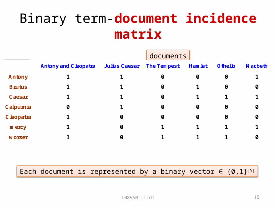
Binary term-document incidence matrix

Antony and Cleopatra Julius Caesar The Tempest Hamlet Othello Macbeth

Antony 1 1 0 0 0 1

Brutus 1 1 0 1 0 0

Caesar 1 1 0 1 1 1

Calpurnia 0 1 0 0 0 0

Cleopatra 1 0 0 0 0 0

mercy 1 0 1 1 1 1

worser 1 0 1 1 1 0

Each document is represented by a binary vector {0,1}∈ |V|

documentswords

L08VSM-tfidf 16

Term-document count matrices

• Consider the number of occurrences of a term in a document: – Each document is a count vector in ℕv

Antony and Cleopatra Julius Caesar The Tempest Hamlet Othello Macbeth

Antony 157 73 0 0 0 0

Brutus 4 157 0 1 0 0

Caesar 232 227 0 2 1 1

Calpurnia 0 10 0 0 0 0

Cleopatra 57 0 0 0 0 0

mercy 2 0 3 5 5 1

worser 2 0 1 1 1 0

17

Bag of words model

• Vector representation doesn’t consider the ordering of words in a document– D1: John is quicker than Mary and D2: Mary is

quicker than John have the same vectors• This is called (as we said in previous lessons)

the bag of words model.– In a sense, this is a step back: the positional index

(see lectures on indexing) was able to distinguish these two documents.

18

Term frequency tf

• The term frequency tft,d of term t in document d is defined as the number of times that t occurs in d.

• We want to use tf when computing query-document match scores. But how?

• Raw term frequency is not what we want:• A document with 10 occurrences of the term may be more

relevant than a document with one occurrence of the term.• But not 10 times more relevant.

• Relevance does not increase proportionally with term frequency.

L08VSM-tfidf 19

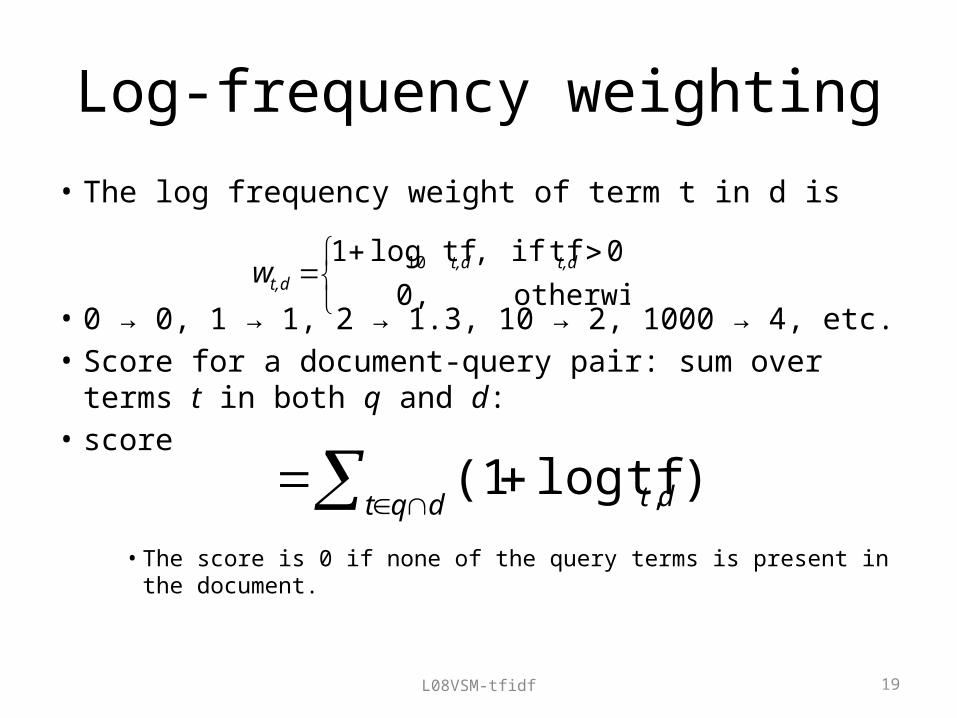
Log-frequency weighting

• The log frequency weight of term t in d is

• 0 → 0, 1 → 1, 2 → 1.3, 10 → 2, 1000 → 4, etc.• Score for a document-query pair: sum over terms t in

both q and d:• score

• The score is 0 if none of the query terms is present in the document.

otherwise 0,

0 tfif, tflog 1 10 t,dt,d

t,dw

dqt dt ) tflog (1 ,

L08VSM-tfidf 20

Document frequency

• Rare terms are more informative than frequent terms

– Recall stop words!

– Consider a term in the query that is rare in the collection (e.g., arachnocentric)

– A document containing this term is very likely to be relevant to the query arachnocentric

– → We want a higher weight for rare terms like arachnocentric.

21

Document frequency, continued

• Consider a query term that is frequent in the collection (e.g., high, increase, line)– A document containing such a term is more likely to be relevant

than a document that doesn’t, but it’s not a sure indicator of relevance.

– → For frequent terms, we want positive weights for words like high, increase, and line, but lower weights than for rare terms.

• We will use document frequency (df) to capture this in the score.

• df ( N) is the number of documents that contain the term

L08VSM-tfidf 22

idf weight

• dft is the document frequency of t: the number of documents that contain t– df is a measure of the informativeness of t

• We define the idf (inverse document frequency) of t by

– We use log N/dft instead of N/dft to “dampen” the effect of idf.

tt N/df log idf 10

Will turn out that the base of the log is immaterial.

L08VSM-tfidf 23

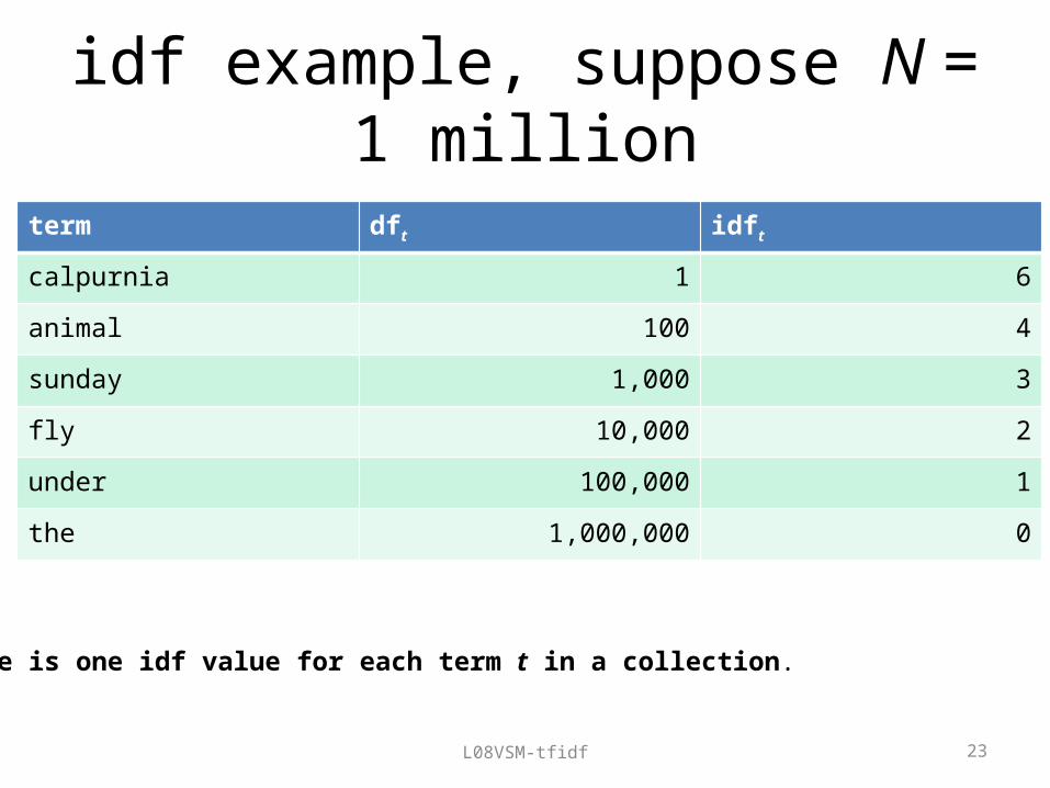
idf example, suppose N = 1 million

term dft idft

calpurnia 1 6

animal 100 4

sunday 1,000 3

fly 10,000 2

under 100,000 1

the 1,000,000 0

There is one idf value for each term t in a collection.

L08VSM-tfidf 24

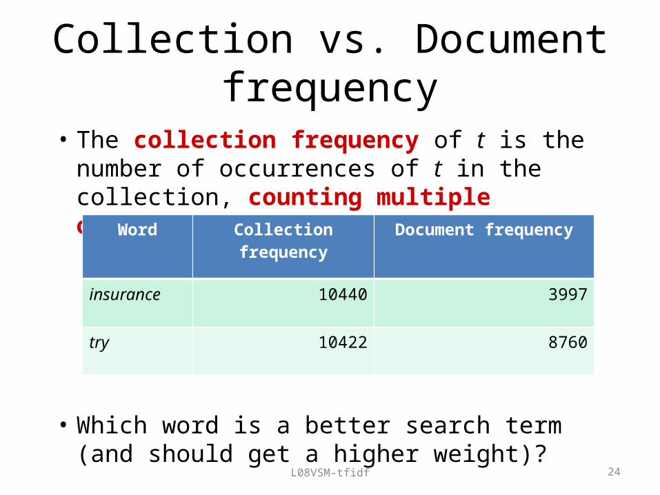
Collection vs. Document frequency

• The collection frequency of t is the number of occurrences of t in the collection, counting multiple occurrences.

• Which word is a better search term (and should get a higher weight)?

Word Collection frequency Document frequency

insurance 10440 3997

try 10422 8760

L08VSM-tfidf 25

tf-idf weighting

• The tf-idf weight of a term is the product of its tf weight and its idf weight.

• Best known weighting scheme in information retrieval• Note: the “-” in tf-idf is a hyphen, not a minus sign!• Alternative names: tf.idf, tf x idf

• Increases with the number of occurrences within a document

• Increases with the rarity of the term in the collection

tdt Ndt

df/log)tflog1(w ,,

L08VSM-tfidf 26

Binary → count → weight matrix

Antony and Cleopatra Julius Caesar The Tempest Hamlet Othello Macbeth

Antony 5.25 3.18 0 0 0 0.35

Brutus 1.21 6.1 0 1 0 0

Caesar 8.59 2.54 0 1.51 0.25 0

Calpurnia 0 1.54 0 0 0 0

Cleopatra 2.85 0 0 0 0 0

mercy 1.51 0 1.9 0.12 5.25 0.88

worser 1.37 0 0.11 4.15 0.25 1.95

Each document is now represented by a real-valued vector of tf-idf weights ∈R|V|

L08VSM-tfidf 27

Documents as vectors

• So we have a |V|-dimensional vector space• Terms are axes of the space• Documents are points or vectors in this space

• Very high-dimensional: hundreds of millions of dimensions when you apply this to a web search engine

• This is a very sparse vector - most entries are zero.

L08VSM-tfidf 28

Queries as vectors

• Key idea 1: Do the same for queries: represent them as vectors in the space

• Key idea 2: Rank documents according to their proximity to the query in this space

• proximity = similarity of vectors• proximity ≈ inverse of distance• Recall: We do this because we want to get away from

the you’re-either-in-or-out Boolean model.• Instead: rank more relevant documents higher than

less relevant documents

L08VSM-tfidf 29

Formalizing vector space proximity

• First cut: distance between two points– ( = distance between the end points of the two

vectors)• Euclidean distance?

• Euclidean distance is a bad idea . . .• . . . because Euclidean distance is large for

vectors of different lengths.

30

Why Euclidean distance is a bad idea

The Euclidean distance between qand d2 is large even though thedistribution of terms in the query q and the distribution ofterms in the document d2 are

very similar.

L08VSM-tfidf 31

Use angle instead of distance

• Experiment: take a document d and append it to itself. Call this document d .′

• “Semantically” d and d have the same content′• The Euclidean distance between the two documents

can be quite large (word frequency doubles in d’)• The angle between the two documents is 0,

corresponding to maximal similarity.• Key idea: Rank documents according to angle with

query.

L08VSM-tfidf 32

From angles to cosines

• The following two notions are equivalent.– Rank documents in decreasing order of the angle

between query and document– Rank documents in increasing order of

cosine(query,document)

• Cosine is a monotonically decreasing function for the interval [0o, 180o]

L08VSM-tfidf 33

Length normalization

• A vector can be (length-) normalized by dividing each of its components by its length – for this we use the L2 norm:

– Dividing a vector by its L2 norm makes it a unit (length) vector

– Effect on the two documents d and d (d appended to ′itself) from earlier slide: they have identical vectors after length-normalization.

i ixx 2

2

34

cosine(query,document)

V

i i

V

i i

V

i ii

dq

dq

d

d

q

q

dq

dqdq

1

2

1

2

1),cos(

Dot product Unit vectors

qi is the tf-idf weight of term i in the querydi is the tf-idf weight of term i in the documentcos(q,d) is the cosine similarity of q and d … or,equivalently, the cosine of the angle between q and d.

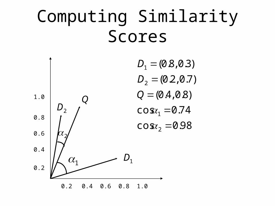
Computing Similarity Scores

2

1 1D

Q2D

98.0cos

74.0cos

)8.0 ,4.0(

)7.0 ,2.0(

)3.0 ,8.0(

2

1

2

1

Q

D

D

1.0

0.8

0.6

0.8

0.4

0.60.4 1.00.2

0.2

Documents in Vector Space

t1

t2

t3D1

D2

D10

D3

D9

D4

D7

D8

D5

D11

D6

L08VSM-tfidf 37

Cosine similarity amongst 3 documents

term SaS PaP WH

affection 115 58 20

jealous 10 7 11

gossip 2 0 6

wuthering 0 0 38

How similar arethe novelsSaS: Sense andSensibilityPaP: Pride andPrejudice, andWH: WutheringHeights?

Term frequencies (counts)

3 documents example contd.

Log frequency weighting

term SaS PaP WH

affection 3.06 2.76 2.30

jealous 2.00 1.85 2.04

gossip 1.30 0 1.78

wuthering 0 0 2.58

After normalization

term SaS PaP WH

affection 0.789 0.832 0.524

jealous 0.515 0.555 0.465

gossip 0.335 0 0.405

wuthering 0 0 0.588

cos(SaS,PaP) ≈0.789 0.832 + 0.515 0.555 + 0.335 0.0 + 0.0 0.0∗ ∗ ∗ ∗≈ 0.94cos(SaS,WH) ≈ 0.79cos(PaP,WH) ≈ 0.69

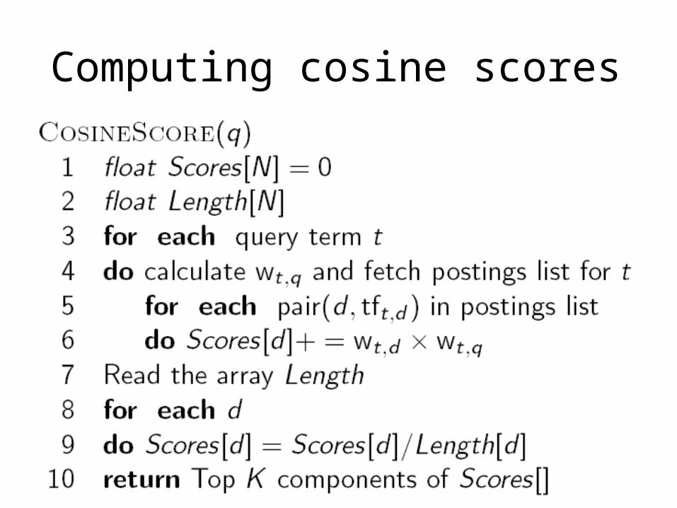
Computing cosine scores

tf-idf weighting has many variants

41

Weighting may differ in queries vs documents

• Many search engines allow for different weightings for queries vs documents

• To denote the combination in use in an engine, we use the notation qqq.ddd with the acronyms from the previous table

• Example: ltn.lnc means:– Query: logarithmic tf (l in leftmost column), idf (t in

second column), no normalization …– Document logarithmic tf, no idf and cosine

normalization

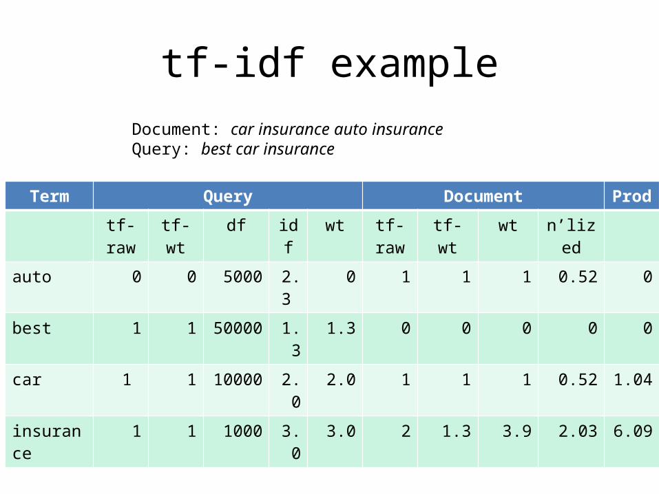
tf-idf example

Term Query Document Prod

tf-raw tf-wt df idf wt tf-raw tf-wt wt n’lized

auto 0 0 5000 2.3 0 1 1 1 0.52 0

best 1 1 50000 1.3 1.3 0 0 0 0 0

car 1 1 10000 2.0 2.0 1 1 1 0.52 1.04

insurance 1 1 1000 3.0 3.0 2 1.3 3.9 2.03 6.09

Document: car insurance auto insuranceQuery: best car insurance

43

Summary – vector space ranking

• Represent the query as a weighted tf-idf vector• Represent each document as a weighted tf-idf

vector

• Compute the cosine similarity score for the query vector and each document vector

• Rank documents with respect to the query by score

• Return the top K (e.g., K = 10) to the user

44

Summary: What’s the point of using vector spaces?

• A well-formed algebraic space for retrieval• Query becomes a vector in the same space as

the docs.– Can measure each doc’s proximity to it.

• Natural measure of scores/ranking – no longer Boolean.– Documents and queries are expressed as bags of

words

45

The Vector Model

• Non-binary (numeric) term weights used to compute degree of similarity between a query and each of the documents.

• Enablespartial matches

• to deal with incompleteness answer set ranking

• to deal with information overload

46

The Vector Model : Pros and Cons

• Advantages:term-weighting improves answer set quality partial matching allows retrieval of docs that

approximate the query conditionscosine ranking formula sorts documents according

to degree of similarity to the query• Disadvantages:

assumes independence of index terms; not clear that this is bad though

Google ranking method

• Ranking is based on the content and on the specific page (later in this course, PageRank)

• Basically, keywords are interpreted as a boolean AND search (advanced options for complex boolean queries)

• However, answers are returned even if a word is not included (basically, it is a mixed boolean-vector space model)

• Additionally, query words are spell-corrected, and additional words can be added (see Query Expansion)