Basic Regression with Time Series DataECONOMETRICS (ECON 360)

BEN VAN KAMMEN, PHD

IntroductionThis chapter departs from the cross-sectional data analysis, which has been the focus in the preceding chapters.

Instead of observing many (“n”) elements in a single time period, time series data are generated by observing a single element over many time periods.

The goal of the chapter is broadly to show what can be done with OLS using time series data.

Specifically students will identify similarities in and differences between the two applications and practice methods unique to time series models.

OutlineThe Nature of Time Series Data.

Stationary and Weakly Dependent Time Series.

Asymptotic Properties of OLS.

Using Highly Persistent Time Series in Regression Analysis.

Examples of (Multivariate) Time Series Regression Models.

Trends and Seasonality.

The nature of time series dataTime series observations have a meaningful order imposed on them, from first to last, in contrast to sorting a cross-section alphabetically or by an arbitrarily assigned ID number.

The values are generated by a stochastic process, about which assumptions can be made, e.g., the mean, variance, covariance, and distribution of the “innovations” (also sometimes called disturbances or shocks) that move the process forward through time.

The nature of time series data (continued)So an observation of a time series, e.g.,

𝑦𝑦𝑡𝑡 ; 𝑡𝑡 ∈ 0, . . . ,𝑛𝑛 , where 𝑛𝑛 is the sample size,

can be thought of as a single realization of the stochastic process.◦ Were history to be repeated, many other realizations for the path of 𝑦𝑦𝑡𝑡 would be possible.

Owing to the randomness generating the observations of y, the properties of OLS that depend on random sampling still hold.

The econometrician’s job is to accurately model the stochastic process, both for the purpose of inference as well as prediction.◦ Prediction is an application for time series model estimates because knowing the process generating

new observations of y naturally enables you to estimate a future (“out of sample”) value.

Stationary and weakly dependent time seriesMany time series processes can be viewed either as ◦ regressions on lagged (past) values with additive disturbances or◦ as aggregations of a history of innovations.

In order to show this, we have to write down a model and make some assumptions about how present values of y (𝑦𝑦𝑡𝑡) are related to past values (e.g., 𝑦𝑦𝑡𝑡−1) and about the variance and covariance structure of the disturbances.

For the sake of clarity, consider a univariate series that does not depend on values of other variables—only on lagged values of itself.

Stationary and weakly dependent time series (continued)

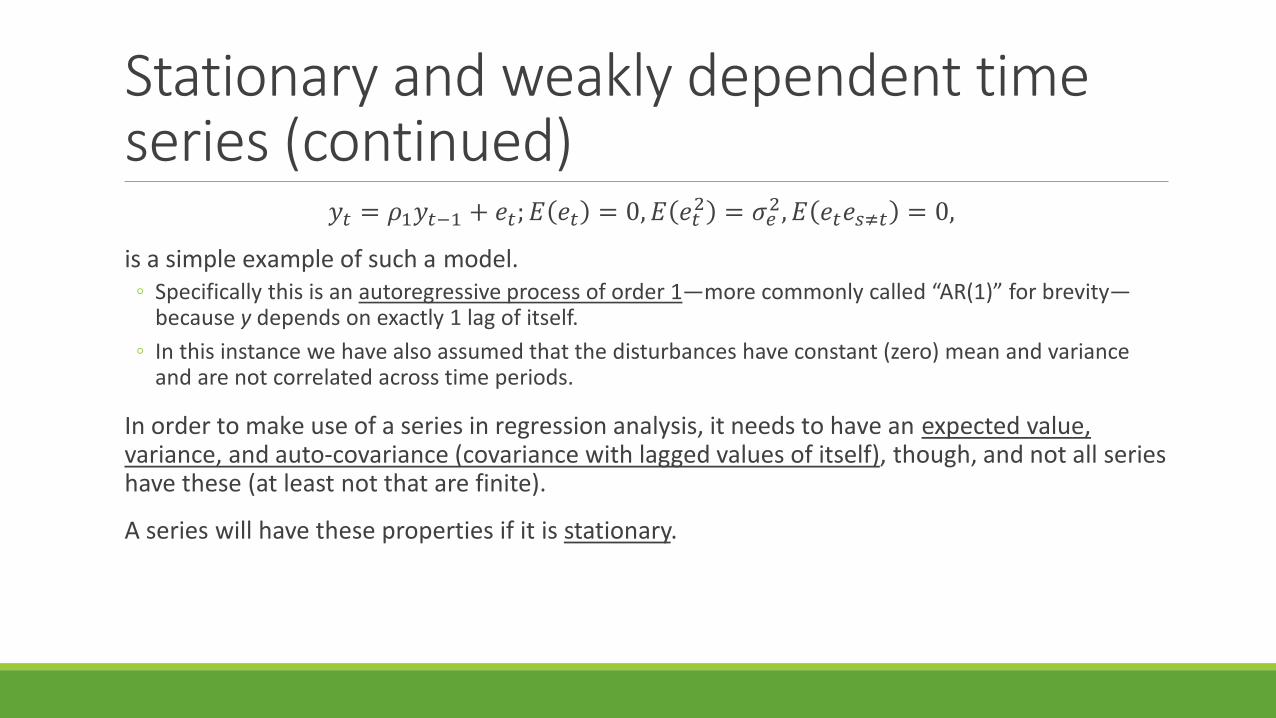
𝑦𝑦𝑡𝑡 = 𝜌𝜌1𝑦𝑦𝑡𝑡−1 + 𝑒𝑒𝑡𝑡;𝐸𝐸 𝑒𝑒𝑡𝑡 = 0,𝐸𝐸 𝑒𝑒𝑡𝑡2 = 𝜎𝜎𝑒𝑒2,𝐸𝐸 𝑒𝑒𝑡𝑡𝑒𝑒𝑠𝑠≠𝑡𝑡 = 0,

is a simple example of such a model.◦ Specifically this is an autoregressive process of order 1—more commonly called “AR(1)” for brevity—

because y depends on exactly 1 lag of itself.◦ In this instance we have also assumed that the disturbances have constant (zero) mean and variance

and are not correlated across time periods.

In order to make use of a series in regression analysis, it needs to have an expected value, variance, and auto-covariance (covariance with lagged values of itself), though, and not all series have these (at least not that are finite).

A series will have these properties if it is stationary.

StationarityThe property of stationarity implies:

1 𝐸𝐸 𝑦𝑦𝑡𝑡 is independent of 𝑡𝑡,

2 𝑉𝑉𝑉𝑉𝑉𝑉 𝑦𝑦𝑡𝑡 is a finite positive constant, independent of 𝑡𝑡,

3 𝐶𝐶𝐶𝐶𝐶𝐶 𝑦𝑦𝑡𝑡 ,𝑦𝑦𝑡𝑡−𝑠𝑠 is a finite function of 𝑡𝑡 − 𝑠𝑠 , but not 𝑡𝑡 or 𝑠𝑠,

4 The distribution of 𝑦𝑦𝑡𝑡 is not changing over time.

For our purposes the 4th condition is unnecessary, and a process that satisfies the first 3 is still weakly stationary or covariance stationary.

Stationarity of AR(1) processThe AR(1) process, 𝑦𝑦𝑡𝑡, is covariance stationary under specific conditions.

𝐸𝐸 𝑦𝑦𝑡𝑡 = 𝜌𝜌1𝐸𝐸 𝑦𝑦𝑡𝑡−1 + 𝐸𝐸 𝑒𝑒𝑡𝑡 ; 1 → 𝐸𝐸 𝑦𝑦𝑡𝑡 = 𝜌𝜌1𝐸𝐸 𝑦𝑦𝑡𝑡 ⇔ 𝐸𝐸 𝑦𝑦𝑡𝑡 = 0,

𝑉𝑉𝑉𝑉𝑉𝑉 𝑦𝑦𝑡𝑡 = 𝐸𝐸 𝑦𝑦𝑡𝑡2 = 𝐸𝐸 𝜌𝜌12𝑦𝑦𝑡𝑡−12 + 𝑉𝑉𝑉𝑉𝑉𝑉 𝑒𝑒𝑡𝑡 = 𝜌𝜌12𝐸𝐸 𝑦𝑦𝑡𝑡2 + 𝜎𝜎𝑒𝑒2,

⇔ 𝑉𝑉𝑉𝑉𝑉𝑉 𝑦𝑦𝑡𝑡 ≡ 𝜎𝜎𝑦𝑦2 =𝜎𝜎𝑒𝑒2

1 − 𝜌𝜌12.

This is only finite if 𝜌𝜌1is less than one in absolute value.◦ Otherwise the denominator goes to zero and the variance goes to infinity.

𝜎𝜎𝑦𝑦2 =𝜎𝜎𝑒𝑒2

1 − 𝜌𝜌12; 𝜌𝜌1 < 1.

Using highly persistent time series in regression analysisEven if the weak dependency assumption fails, i.e., 𝜌𝜌1 = 1, an autoregressive process can be analyzed using a (1st difference) transformed OLS model, which makes a non-stationary, strongly dependent process stationary.◦ The differences in the following process (called a “random walk”) are stationary.

𝑦𝑦𝑡𝑡 = 1 ∗ 𝑦𝑦𝑡𝑡−1 + 𝑒𝑒𝑡𝑡 → ∆𝑦𝑦𝑡𝑡 ≡ 𝑦𝑦𝑡𝑡 − 𝑦𝑦𝑡𝑡−1 = 𝑒𝑒𝑡𝑡,

has a finite mean and variance (distribution) that does not depend on t.

The Wooldridge book contains more information on testing whether a series has this kind of persistence (see pp. 396-399 and 639-644) and selecting an appropriate transformation of the regression model, but these topics are left to the interested student as optional.

Stationarity of AR(1) process (continued)The covariance between two observations that are h periods apart is:

𝐸𝐸 𝑦𝑦𝑡𝑡𝑦𝑦𝑡𝑡+ℎ = 𝜎𝜎𝑦𝑦2𝜌𝜌1ℎ.

This “auto-covariance” does not depend on either of the two places in the time series—only on how far apart they are.◦ To derive this, one needs to iteratively substitute for 𝑦𝑦𝑡𝑡+1:

𝑦𝑦𝑡𝑡+1 = 𝜌𝜌1 𝜌𝜌1𝑦𝑦𝑡𝑡−1 + 𝑒𝑒𝑡𝑡 + 𝑒𝑒𝑡𝑡+1; 𝑦𝑦𝑡𝑡+2 = 𝜌𝜌1[ 𝜌𝜌12𝑦𝑦𝑡𝑡−1 + 𝜌𝜌1𝑒𝑒𝑡𝑡 + 𝑒𝑒𝑡𝑡+1] + 𝑒𝑒𝑡𝑡+2.

With careful inspection, a pattern emerges as you continue substituting.

𝑦𝑦𝑡𝑡+ℎ = 𝜌𝜌1ℎ+1𝑦𝑦𝑡𝑡−1 + �𝑠𝑠=0

ℎ

𝜌𝜌1𝑠𝑠𝑒𝑒𝑡𝑡+ℎ−𝑠𝑠 .

More on this derivation.

Stationarity of AR(1) process (concluded)How persistent the series is depends on how close to one 𝜌𝜌1 is in absolute value. ◦ The closer it is, the more persistent are the values in the series.◦ It is also worth noting how the persistence “dies out” when the gap (h) between the observations is

large.◦ This should confirm the intuition that observations with more time intervening between them will be

less correlated.

Before moving on, let’s summarize a couple more things about the iterative substitution of the AR(1) 𝑦𝑦𝑡𝑡 process.

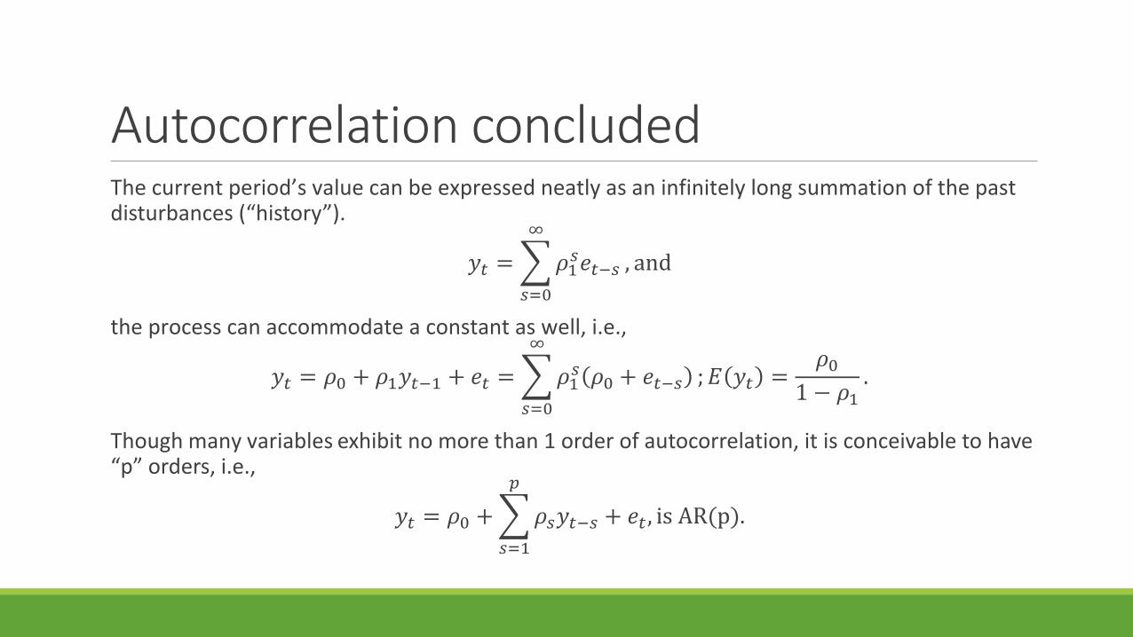
Autocorrelation concludedThe current period’s value can be expressed neatly as an infinitely long summation of the past disturbances (“history”).

𝑦𝑦𝑡𝑡 = �𝑠𝑠=0

∞

𝜌𝜌1𝑠𝑠𝑒𝑒𝑡𝑡−𝑠𝑠 , and

the process can accommodate a constant as well, i.e.,

𝑦𝑦𝑡𝑡 = 𝜌𝜌0 + 𝜌𝜌1𝑦𝑦𝑡𝑡−1 + 𝑒𝑒𝑡𝑡 = �𝑠𝑠=0

∞

𝜌𝜌1𝑠𝑠 𝜌𝜌0 + 𝑒𝑒𝑡𝑡−𝑠𝑠 ;𝐸𝐸 𝑦𝑦𝑡𝑡 =𝜌𝜌0

1 − 𝜌𝜌1.

Though many variables exhibit no more than 1 order of autocorrelation, it is conceivable to have “p” orders, i.e.,

𝑦𝑦𝑡𝑡 = 𝜌𝜌0 + �𝑠𝑠=1

𝑝𝑝

𝜌𝜌𝑠𝑠𝑦𝑦𝑡𝑡−𝑠𝑠 + 𝑒𝑒𝑡𝑡 , is AR(p).

Asymptotic properties of OLSThe assumptions about autoregressive processes made so far lead to disturbances that are contemporaneously exogenous if the parameters were to be estimated by OLS.

This set (next slide) of assumptions leads to Theorem 11.1, which is that OLS estimation of a time series is consistent.

An AR process, for example, will still be biased in finite samples, however, because it violates the stronger Assumption TS.3 (that all disturbances are uncorrelated with all regressors—not just the contemporary one).

More on the biasedness of OLS.

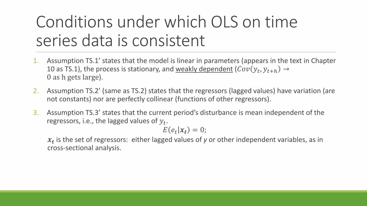
Conditions under which OLS on time series data is consistent

1. Assumption TS.1’ states that the model is linear in parameters (appears in the text in Chapter 10 as TS.1), the process is stationary, and weakly dependent (𝐶𝐶𝐶𝐶𝐶𝐶 𝑦𝑦𝑡𝑡 ,𝑦𝑦𝑡𝑡+ℎ →0 as h gets large).

2. Assumption TS.2’ (same as TS.2) states that the regressors (lagged values) have variation (are not constants) nor are perfectly collinear (functions of other regressors).

3. Assumption TS.3’ states that the current period’s disturbance is mean independent of the regressors, i.e., the lagged values of 𝑦𝑦𝑡𝑡.

𝐸𝐸 𝑒𝑒𝑡𝑡 𝒙𝒙𝒕𝒕 = 0;𝒙𝒙𝒕𝒕 is the set of regressors: either lagged values of y or other independent variables, as in cross-sectional analysis.

Asymptotic properties of OLS (concluded)Under additional Assumptions about the disturbances, inference according to the usual tests is valid:

4. Assumption TS.4’ is the analog of the homoskedasticity assumption:𝑉𝑉𝑉𝑉𝑉𝑉 𝑒𝑒𝑡𝑡|𝒙𝒙𝒕𝒕 = 𝑉𝑉𝑉𝑉𝑉𝑉 𝑒𝑒𝑡𝑡 = 𝜎𝜎2,

which is called contemporaneous homoskedasticity.

5. And Assumption TS.5’ rules out serial correlation in the disturbances:𝐸𝐸 𝑒𝑒𝑡𝑡, 𝑒𝑒𝑡𝑡−ℎ|𝒙𝒙𝒕𝒕,𝒙𝒙𝒕𝒕−𝒉𝒉 = 0|ℎ ≠ 0.

Examples of (multivariate) time series regression modelsThere are numerous time series applications that involve multiple variables moving together over time that this course will not discuss:◦ the interested student should study Chapter 18.

But bringing the discussion of time series data back to familiar realms, consider a simple example in which the dependent variable is a function of contemporaneous and past values of the explanatory variable.

Models that exhibit this trait are called “finite distributed lag” (FDL) models.

Finite distributed lag modelsThis type is further differentiated by its order, i.e., how many lags are relevant for predicting y.

An FDL of order q is written:𝑦𝑦𝑡𝑡 = 𝛼𝛼0 + 𝛿𝛿0𝑧𝑧𝑡𝑡 + 𝛿𝛿1𝑧𝑧𝑡𝑡−1+. . . +𝛿𝛿𝑞𝑞𝑧𝑧𝑡𝑡−𝑞𝑞 + 𝑢𝑢𝑡𝑡 , or compactly as,

𝑦𝑦𝑡𝑡 = 𝛼𝛼0 + �ℎ=0

𝑞𝑞

𝛿𝛿ℎ𝑧𝑧𝑡𝑡−ℎ + 𝑢𝑢𝑡𝑡 .

Note that this contains the “Static Model,” i.e., in which 𝛿𝛿ℎ = 0|ℎ > 0, as a special case.

Applications are numerous. ◦ the fertility (responds to tax code incentives to have children) example in the text ◦ exemplifies short run and long run responses to a market shock.

Finite distributed lag models (continued)In a competitive market, a demand increase will raise prices in the short run but invite entry in the long run, along with its price reducing effects.◦ Also there is a difference between short run and long run demand elasticity; the latter is more elastic. ◦ So the effect of a price change on quantity demanded may be modest in the present but significant over

a longer period of time.

For example demand for gasoline is quite inelastic in the short run but much more elastic in the long run,◦ because consumers can change their vehicles, commuting habits, and locations if given enough time.

These effects could be estimated separately using an FDL model such as:𝑓𝑓𝑢𝑢𝑒𝑒𝑙𝑙𝑡𝑡 = 𝛼𝛼0 + 𝛿𝛿0𝑝𝑝𝑉𝑉𝑝𝑝𝑝𝑝𝑒𝑒𝑡𝑡 + 𝛿𝛿1𝑝𝑝𝑉𝑉𝑝𝑝𝑝𝑝𝑒𝑒𝑡𝑡−1+. . . +𝛿𝛿𝑞𝑞𝑝𝑝𝑉𝑉𝑝𝑝𝑝𝑝𝑒𝑒𝑡𝑡−𝑞𝑞 + 𝑢𝑢𝑡𝑡 .

Finite distributed lag models (concluded)The familiar prediction from microeconomics is that the static effect—sometimes called the impact multiplier—is quite small or zero while the overall effect—the equilibrium multiplier—of a price increase is large and negative.

Formally these could be stated:

𝛿𝛿0 ≈ 0 and �ℎ=0

𝑞𝑞

𝛿𝛿ℎ < 0.

For the long run or “equilibrium” multiplier, one wants to examine the cumulative (sum of the) effects, as a persistently higher price continues to reduce quantity demanded over time periods. ◦ This is the effect of a permanent increase, as described in the text on page 348.

Trends and seasonalityA common source of omitted variable bias in a time series regression is time, itself.

If two variables are trending in the same (opposite) direction over time, they will appear related if time is omitted from the regression.◦ This is true even when there is no substantive relationship between the two variables.◦ Many examples here.

To model a time trend in 𝑦𝑦 that increases it by a constant amount (𝛼𝛼1) each period.𝑦𝑦𝑡𝑡 = 𝛼𝛼0 + 𝛼𝛼1𝑡𝑡 + 𝑒𝑒𝑡𝑡 → ∆𝑦𝑦𝑡𝑡 = 𝛼𝛼0 + 𝛼𝛼1𝑡𝑡 + 𝑒𝑒𝑡𝑡 − 𝛼𝛼0 + 𝛼𝛼1 𝑡𝑡 − 1 + 𝑒𝑒𝑡𝑡−1 ,

⇔ ∆𝑦𝑦𝑡𝑡 = 𝛼𝛼1 𝑡𝑡 − 𝑡𝑡 + 1 + 𝑒𝑒𝑡𝑡 − 𝑒𝑒𝑡𝑡−1 = 𝛼𝛼1 + ∆𝑒𝑒𝑡𝑡.

Trends and seasonality (continued)The difference in consecutive errors has an expectation of zero, so 𝛼𝛼1is the expected change per period.

Were 𝑦𝑦𝑡𝑡 to grow at a constant rate instead of by a constant amount each period, the semi-log specification would more accurately capture the time trend, i.e.,

ln 𝑦𝑦𝑡𝑡 = 𝛼𝛼0 + 𝛼𝛼1𝑡𝑡 + 𝑒𝑒𝑡𝑡 → ∆ln 𝑦𝑦𝑡𝑡 = 𝛼𝛼1 ≈∆𝑦𝑦𝑡𝑡𝑦𝑦𝑡𝑡−1

.

This is the (expected) growth rate of y per period: y grows at 100 ∗ 𝛼𝛼1% per period.

To contrast the two varieties of time trends, observe the following two figures.

Time trends illustrated (1)

Figure 1: Linear Trend

Time trend illustrated (2)

Figure 1: Exponential Trend

Time trends and seasonality (continued)Accounting for the time trend when regressing two time series variables avoids the omitted variable problem that would result from estimating the model,

𝑦𝑦𝑡𝑡 = 𝛽𝛽0 + 𝛽𝛽1𝑥𝑥𝑡𝑡1 + 𝛽𝛽2𝑥𝑥𝑡𝑡2 + 𝛽𝛽3𝑡𝑡 + 𝑢𝑢𝑡𝑡 ,

using only the x variables, thus generating biased estimates of their coefficients.

A detrending interpretation of regressions with a time trendWere the researcher to “de-trend” all of the variables prior to performing the above regression, however, the estimates would not be biased.

By “de-trending” what is meant is to regress each of them on time and subtract the fitted values—so store the residuals. ◦ The following example will illustrate this.

Suppose one regressed a time series of employment in a local area (San Francisco, CA) observations on a time series of the minimum wage.

Detrending (continued)The results would look like this.

The positive coefficient estimate seems to contradict the usual theoretical prediction that a wage floor decreases equilibrium employment.However both variables trend upward over time, as the following regressions demonstrates.

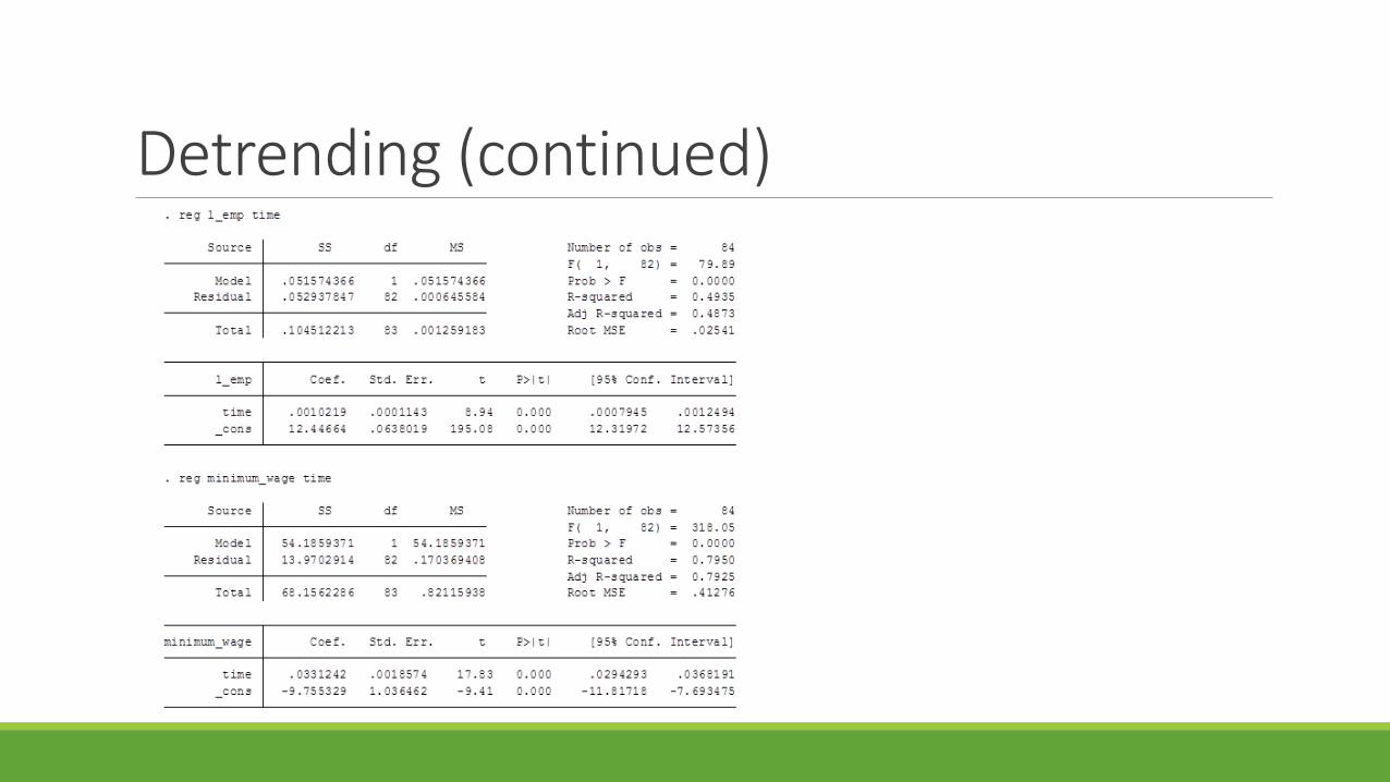
Detrending (continued)

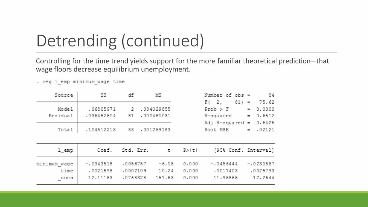
Detrending (continued)Controlling for the time trend yields support for the more familiar theoretical prediction—that wage floors decrease equilibrium unemployment.

Detrending (concluded)The following Stata code would enable you to obtain the same results using de-trended variables.reg l_emp timepredict l_emp_detr, residualsreg minimum_wage timepredict mw_detr, residuals

Then you could regress the residuals on one another (without the time trend) to obtain the estimates without the bias of the omitted time trend.

SeasonalityThe same statements about time trends can be made about seasonal (calendar period-specific) effects:◦ variables that move in predictable ways through the calendar year.◦ These can be accounted for using seasonal indicator variables, e.g.,

𝑚𝑚𝑉𝑉𝑉𝑉𝑝𝑝ℎ𝑡𝑡 = �1, month of observation is 𝑀𝑀𝑉𝑉𝑉𝑉𝑝𝑝ℎ0, otherwise.

Including a set of monthly (quarterly) indicators in a regression accomplishes the same thing as including a time trend:◦ controlling for a spurious variable that would otherwise bias the estimates.

The same process that works with trends works with seasonality: “de-seasonalizing” of variables.

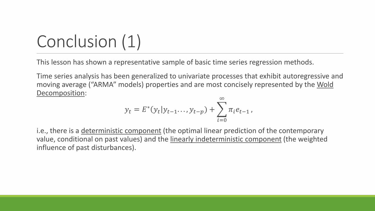
Conclusion (1)This lesson has shown a representative sample of basic time series regression methods.

Time series analysis has been generalized to univariate processes that exhibit autoregressive and moving average (“ARMA” models) properties and are most concisely represented by the WoldDecomposition:

𝑦𝑦𝑡𝑡 = 𝐸𝐸∗ 𝑦𝑦𝑡𝑡 𝑦𝑦𝑡𝑡−1. . . ,𝑦𝑦𝑡𝑡−𝑝𝑝) + �𝑖𝑖=0

∞

𝜋𝜋𝑖𝑖𝑒𝑒𝑡𝑡−1 ,

i.e., there is a deterministic component (the optimal linear prediction of the contemporary value, conditional on past values) and the linearly indeterministic component (the weighted influence of past disturbances).

Conclusion (2)Other directions for more thorough examination by the interested student include:

1. Descriptive measures of autocorrelation, e.g., the autocovariance function and partial autocorrelation coefficients, and the correlogram.

2. Tests for autocorrelation, e.g., the Durbin-Watson Test, Godfrey-Breusch Test, and Box-Pierce Test.

3. Heteroskedasticity robust inference about time series estimates.

4. Tests for the order of integration of a process.

5. The use of time series models for out of sample prediction (“forecasting”).

Collectively these topics would consume far more time that we have in this course. The interested student is advised to indulge any interest in a course such as ECON 573 (Financial Econometrics).

Optional: autocovariance of AR(1) process

𝑦𝑦𝑡𝑡𝑦𝑦𝑡𝑡+ℎ = 𝜌𝜌1ℎ+1𝑦𝑦𝑡𝑡−1 + �𝑠𝑠=0

ℎ

𝜌𝜌1𝑠𝑠𝑒𝑒𝑡𝑡+ℎ−𝑠𝑠 𝜌𝜌1𝑦𝑦𝑡𝑡−1 + 𝑒𝑒𝑡𝑡

= 𝜌𝜌1ℎ+2𝑦𝑦𝑡𝑡−12 + 𝑦𝑦𝑡𝑡−1�𝑠𝑠=0

ℎ

𝜌𝜌1𝑠𝑠+1𝑒𝑒𝑡𝑡+ℎ−𝑠𝑠 + 𝜌𝜌1ℎ+1𝑦𝑦𝑡𝑡−1𝑒𝑒𝑡𝑡 + 𝑒𝑒𝑡𝑡�𝑠𝑠=0

ℎ

𝜌𝜌1𝑠𝑠𝑒𝑒𝑡𝑡+ℎ−𝑠𝑠 .

Take the expectation of this to find the covariance.

Optional: autocovariance of AR(1) process (continued)

𝐶𝐶𝐶𝐶𝐶𝐶 𝑦𝑦𝑡𝑡 ,𝑦𝑦𝑡𝑡+ℎ = 𝐸𝐸 𝑦𝑦𝑡𝑡𝑦𝑦𝑡𝑡+ℎ

= 𝜌𝜌1ℎ+2𝐸𝐸 𝑦𝑦𝑡𝑡−12 + 𝐸𝐸 𝑦𝑦𝑡𝑡−1 �𝑠𝑠=0

ℎ

𝜌𝜌1𝑠𝑠+1𝑒𝑒𝑡𝑡+ℎ−𝑠𝑠 + 𝜌𝜌1ℎ+1𝐸𝐸 𝑦𝑦𝑡𝑡−1𝑒𝑒𝑡𝑡 + 𝐸𝐸 𝑒𝑒𝑡𝑡�𝑠𝑠=0

ℎ

𝜌𝜌1𝑠𝑠𝑒𝑒𝑡𝑡+ℎ−𝑠𝑠 ,

in which (fortunately) most of the terms are uncorrelated:

𝐸𝐸 𝑦𝑦𝑡𝑡𝑦𝑦𝑡𝑡+ℎ = 𝜌𝜌1ℎ+2𝜎𝜎𝑦𝑦2 + 0 + 0 + 𝐸𝐸 𝑒𝑒𝑡𝑡�𝑠𝑠=0

ℎ

𝜌𝜌1𝑠𝑠𝑒𝑒𝑡𝑡+ℎ−𝑠𝑠 = 𝜌𝜌1ℎ+2𝜎𝜎𝑦𝑦2 + 𝜌𝜌1ℎ𝜎𝜎𝑒𝑒2,

where the 2nd equality uses the assumption that the disturbances are uncorrelated across time periods.

𝐸𝐸 𝑒𝑒𝑡𝑡𝑒𝑒𝑡𝑡+ℎ−𝑠𝑠 = �𝜎𝜎𝑒𝑒2, 𝑠𝑠 = ℎ

0, 𝑠𝑠 ≠ ℎ.

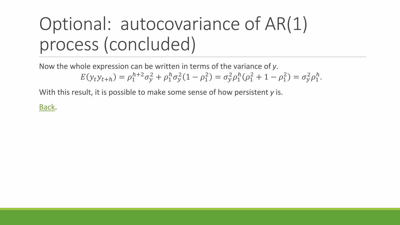
Optional: autocovariance of AR(1) process (concluded)Now the whole expression can be written in terms of the variance of y.

𝐸𝐸 𝑦𝑦𝑡𝑡𝑦𝑦𝑡𝑡+ℎ = 𝜌𝜌1ℎ+2𝜎𝜎𝑦𝑦2 + 𝜌𝜌1ℎ𝜎𝜎𝑦𝑦2 1 − 𝜌𝜌12 = 𝜎𝜎𝑦𝑦2𝜌𝜌1ℎ 𝜌𝜌12 + 1 − 𝜌𝜌12 = 𝜎𝜎𝑦𝑦2𝜌𝜌1ℎ.

With this result, it is possible to make some sense of how persistent y is.

Back.

Optional: biasedness of OLSThe proof of this is fairly complex, but intuitively the bias comes from the fact that the present period disturbance 𝑒𝑒𝑡𝑡 can be expressed as a function of lagged values of the dependent variable; ◦ these are correlated with the regressor, 𝑦𝑦𝑡𝑡−1, resulting in the bias in finite samples.

But the OLS bias with lagged dependent variables as regressor does disappear with large samples,◦ so at least OLS is consistent in these circumstances.

Optional: biasedness of OLS (sketch of “proof”)The estimator of 𝜌𝜌 in an AR(1) regression is:

�𝜌𝜌1 = 𝜌𝜌1 +∑𝑡𝑡=1𝑛𝑛 𝑦𝑦𝑡𝑡−1𝑒𝑒𝑡𝑡∑𝑡𝑡=1𝑛𝑛 𝑦𝑦𝑡𝑡−12 .

𝑒𝑒𝑡𝑡 can be written using a lag operator, 1 − 𝜌𝜌1𝐿𝐿 𝑦𝑦𝑡𝑡 = 𝑦𝑦𝑡𝑡 − 𝜌𝜌1𝑦𝑦𝑡𝑡−1.

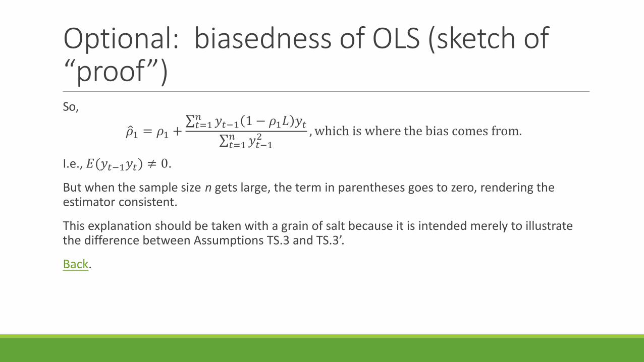
Optional: biasedness of OLS (sketch of “proof”)So,

�𝜌𝜌1 = 𝜌𝜌1 +∑𝑡𝑡=1𝑛𝑛 𝑦𝑦𝑡𝑡−1 1 − 𝜌𝜌1𝐿𝐿 𝑦𝑦𝑡𝑡

∑𝑡𝑡=1𝑛𝑛 𝑦𝑦𝑡𝑡−12 , which is where the bias comes from.

I.e., 𝐸𝐸(𝑦𝑦𝑡𝑡−1𝑦𝑦𝑡𝑡) ≠ 0.

But when the sample size n gets large, the term in parentheses goes to zero, rendering the estimator consistent.

This explanation should be taken with a grain of salt because it is intended merely to illustrate the difference between Assumptions TS.3 and TS.3’.

Back.