Basic Statistical Inference for Survey Data

Professor Ron FrickerNaval Postgraduate School

Monterey, California

1

Goals for this Lecture

• Review of descriptive statistics • Review of basic statistical inference

– Point estimation– Sampling distributions and the standard error– Confidence intervals for the mean– Hypothesis tests for the mean

• Compare and contrast classical statistical assumptions to survey data requirements

• Discuss how to adapt methods to survey data with basic sample designs

2

Two Roles of Statistics

• Descriptive: Describing a sample or population– Numerical: (mean, variance, mode)

– Graphical: (histogram, boxplot)

• Inferential: Using a sample to infer facts about a population– Estimating (e.g., estimating the average starting salary of

those with systems engineering Master’s degrees)

– Testing theories (e.g., evaluating whether a Master’s degree increases income)

– Building models (e.g., modeling the relationship of how an advanced degree increases income)

A Descriptive Statistics Question: What was the average survey response to question 7?

An Inferential Question: Given the sample, what can we say about the average response to question 7 for the population?

Lots of Descriptive Statistics

• Numerical:– Measures of location

• Mean, median, trimmed mean, percentiles

– Measures of variability• Variance, standard deviation,

range, inter-quartile range– Measures for categorical data

• Mode, proportions

• Graphical– Continuous: Histograms, boxplots, scatterplots– Categorical: Bar charts, pie charts

Continuous Data: Sample Mean, Variance, and Standard Deviation

• Sample average or sample mean is a measure of location or central tendency:

• Sample variance is a measure of variability

• Standard deviation is the square root of the variance

1

1 n

ii

x xn =

= ∑

2 2

1

1 ( )1

n

ii

s x xn =

= −− ∑

2ss =7

Statistical Inference

• Sample mean, , and sample variance, s2, are statistics calculated from data

• Sample statistics used to estimate true value of population called estimators

• Point estimation: estimate a population statistic with a sample statistic

• Interval estimation: estimate a population statistic with an interval– Incorporates uncertainty in the sample statistic

• Hypothesis tests: test theories about the population based on evidence in the sample data

x

8

Classical Statistical Assumptions vs. Survey Practice / Requirements

• Basic statistical methods assume:– Population is of infinite size (or so large as to be

essentially infinite)– Sample size is a small fraction of the population– Sample is drawn from the population via SRS

• In surveys:– Population always finite (though may be very large)– Sample could be sizeable fraction of the population

• “Sizeable” is roughly > 5%– Sampling may be complex

9

Point Estimation (1)

• Example: Use sample mean or proportion to estimate population mean or proportion

• Using SRS or a self-weighting sampling scheme, usual estimators for the mean calculated in all stat software packages are generally fine– Assuming no other adjustments are necessary

• E.g., nonresponse, poststratification, etc• Except under SRS, usual point estimates for

standard deviation almost always wrong10

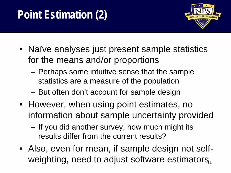
Point Estimation (2)

• Naïve analyses just present sample statistics for the means and/or proportions– Perhaps some intuitive sense that the sample

statistics are a measure of the population– But often don’t account for sample design

• However, when using point estimates, no information about sample uncertainty provided– If you did another survey, how much might its

results differ from the current results?• Also, even for mean, if sample design not self-

weighting, need to adjust software estimators11

Sampling Distributions

• Abstract from people and surveys to random variables and their distributions

12

Sampling Distributions

• Sampling distribution is the probability distribution of a sample statistic

0.0

0.1

0.2

0.3

0.4

0.5

0.6

0.7

0.8

0.9

812 813 814 815 816 817 818Index

IndividualMean of 5

Sampling distribution of means of five

obs

Standard error: 5σσ =X

Distribution individual obswith standard deviation σ

13

Demonstrating Randomness

http://www.ruf.rice.edu/~lane/stat_sim/sampling_dist/index.html

Simulating Sampling Distributions

http://www.ruf.rice.edu/~lane/stat_sim/sampling_dist/index.html

Central Limit Theorem (CLT) for the Sample Mean

• Let X1, X2, …, Xn be a random sample from any distribution with mean µ and standard deviation σ

• For large sample size n, the distribution of the sample mean has approximately a normal distribution – with mean µ, and– standard deviation

• The larger the value of n, the better the approximation

nσ

16

Example: Sums of Dice Rolls

Roll of a Single Die

0

20

40

60

80

100

120

1 2 3 4 5 6

Outcome

Freq

uenc

y

Sum of Two Dice

0

100

200

300

400

500

600

700

2 3 4 5 6 7 8 9 10 11 12Sum

Freq

uenc

y

Sum of 5 Dice

0

10

20

30

40

50

60

70

1 3 5 7 9 11 13 15 17 19 21 23 25

Sum

Freq

uenc

y

Sum of 10 Dice

0

50

100

150

200

250

300

350

5 8 11 14 17 20 23 26 29 32 35 38 41 44 47 50 53 56 59

Sum

Freq

uenc

y

One roll

Sum of 2 rolls

Sum of 5 rolls

Sum of 10 rolls

17

Demonstrating Sampling Distributions and the CLT

http://www.ruf.rice.edu/~lane/stat_sim/sampling_dist/index.html

Interval Estimation for µ

• Best estimate for µ is • But will never be exactly µ

– Further, there is no way to tell how far off• BUT can estimate µ’s location with an interval

and be right some of the time– Narrow intervals: higher chance of being wrong– Wide intervals: less chance of being wrong, but

also less useful• AND with confidence intervals (CIs) can

define the probability the interval “covers” µ!

XX

Confidence Intervals: Main Idea

20

• Alternatively, µ is within 2 s.e.s of 95% of the time

X

0.0

0.1

0.2

0.3

0.4

0.5

0.6

0.7

0.8

0.9

812 813 814 815 816 817 818

Index

Individual

(Unobserved) dist. of population

Mean of 5

(Unobserved) dist. of sample mean

Unobserved pop mean

95% confidence interval for pop mean

• Based on the normal distribution, we know is within 2 s.e.s of µ 95% of the time

X

Sample mean

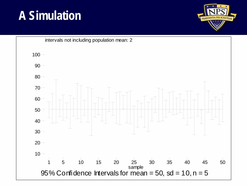
A Simulationintervals not including population mean: 2

95% Confidence Intervals for mean = 50, sd = 10, n = 5sample

1 5 10 15 20 25 30 35 40 45 50

10

20

30

40

50

60

70

80

90

100

Another Simulationintervals not including population mean: 10

95% Confidence Intervals for mean = 50, sd = 10, n = 95sample

1 10 20 30 40 50 60 70 80 90 100 110 120130 140 150160 170 180190 200

20

30

40

50

60

70

80

Confidence Interval for µ (1)

• For from sample of size n from a population with mean µ,

has a t distribution with n-1 “degrees of freedom”– Precisely if population has normal distribution– Approximately for sample mean via CLT

• Use the t distribution to build a CI for the mean:

/XTs n

µ−=

X

( )/ 2, 1 / 2, 1Pr 1n nt T tα α α− −− < < = −

23

Review: the t Distribution

0.00

0.10

0.20

0.30

0.40

-4 -3 -2 -1 0 1 2 3 4

Z= number of SE’s from the mean

normal

T3

T10

T100

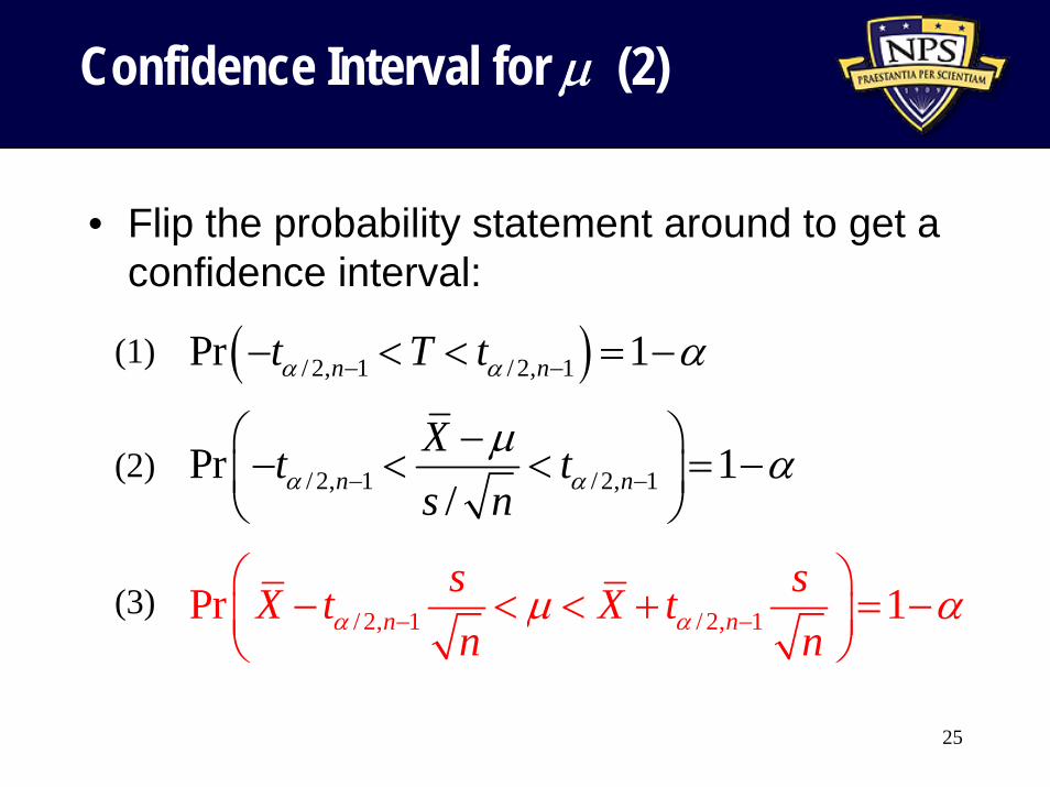
Confidence Interval for µ (2)

• Flip the probability statement around to get a confidence interval:

( )/ 2, 1 / 2, 1Pr 1n nt T tα α α− −− < < = −(1)

/ 2, 1 / 2, 1Pr 1/n n

Xt ts nα α

µ α− −

⎛ ⎞−− < < = −⎜ ⎟

⎝ ⎠(2)

/ 2, 1 / 2, 1Pr 1n ns sX t X tn nα αµ α− −

⎛ ⎞− < < + = −⎜ ⎟⎝ ⎠

(3)

25

Example: Constructing a 95% Confidence Interval for µ

• Choose the confidence level: 1-α• Remember the degrees of freedom (ν) = n -1• Find

– Example: if α = 0.05, df=7 then = 2.365• Calculate and

• Then

X ns /

95.0365.2365.2Pr =⎟⎠

⎞⎜⎝

⎛ +<<−nsX

nsX µ

1,2/ −ntα7,025.0t

Hypothesis Tests

• Basic idea is to test a hypothesis / theory on empirical evidence from a sample– E.g., “The fraction of new students aware of the

school discrimination policy is less than 75%.”– Does the data support or refute the assertion?

27

p̂p=0.75 = 0.832 If we assume this is true, how likely are we to see this

(or something more extreme)?

This is the probability.If it’s small, we don’t

believe our assumption.

One-Sample, Two-sided t-Test

• Hypothesis:H0: µ = µ0

Ha: µ ≠ µ0

• Standardized test statistic:

• p-value = Pr(T<-t and T>t) = Pr(|T|>t), where T follows a t distribution with n-1 degrees of freedom

• Reject H0 if p < α, where α is the predetermined significance level

02 /

Xts n

µ−=

28

One-Sample, One-sided t-Tests

• Hypotheses:H0: µ = µ0 H0: µ = µ0Ha: µ < µ0 Ha: µ > µ0

• Standardized test statistic:

• p-value = Pr(T < t) or p-value = Pr(T > t), depending on Ha, where T follows a tdistribution with n-1 degrees of freedom

• Reject H0 if p < α

02 /

Xts n

µ−=

or

29

Applying Continuous Methods to Binary Survey Questions

• In surveys, often have binary questions, where desire to infer proportion of population in one category or the other

• Code binary question responses as 1/0 variable and for large n appeal to the CLT– Confidence interval for the mean is a CI on the

proportion of “1”s– T-test for the mean is a hypothesis test on the

proportion of “1”s

30

Applying Continuous Methods to Likert Scale Survey Data

• Likert scale data is inherently categorical• If willing to make assumption that “distance”

between categories is equal, then can code with integers and appeal to CLT

Strongly agreeAgreeNeutralDisagreeStrongly disagree

12345

31

Adjusting Standard Errors (for Basic Survey Sample Designs)

• Sample > 5% of population: finite population correction– Multiply the standard error by– E.g.

• Stratified sample, weighted sum of the strata variances:

( ) /N n N−

( ) ( )1

. . /N Var( )H

h hh

s e x N x=

= ∑

. .( ) ( ) / /s e x N n N s n= − ×

32

What We Have Just Reviewed

• Review of descriptive statistics • Review of basic statistical inference

– Point estimation– Sampling distributions and the standard error– Confidence intervals for the mean– Hypothesis tests for the mean

• Compare and contrast classical statistical assumptions to survey data requirements

• Discuss how to adapt methods to survey data with basic sample designs

33