basic statistics. content data types descriptive statistics graphical summaries distributions ...
TRANSCRIPT

Basic Statistics

Content
Data Types
Descriptive Statistics
Graphical Summaries
Distributions
Sampling and Estimation
Confidence Intervals
Hypothesis Testing (Statistical tests)
Errors in Hypothesis Testing
Sample Size

Data Types

Motivation
Defining your data type is always a sensible first consideration
You then know what you can ‘do’ with it

Variables
Quantitative Variable A variable that is counted or measured on a
numerical scale
Can be continuous or discrete (always a whole number).
Qualitative Variable A non-numerical variable that can be classified into
categories, but can’t be measured on a numerical scale.
Can be nominal or ordinal
Continuous Data
Continuous data is measured on a scale.
The data can have almost any numeric value and can be recorded at many different points.
For example:
Temperature (39.25oC)
Time (2.468 seconds)
Height (1.25m)
Weight (66.34kg)

Discrete Data
Discrete data is based on counts, for example:
The number of cars parked in a car park
The number of patients seen by a dentist each day.
Only a finite number of values are possible e.g. a dentist could see 10, 11, 12 people but not 12.3 people

Nominal Data
A Nominal scale is the most basic level of measurement. The variable is divided into categories and objects are ‘measured’ by assigning them to a category.
For example,
Colours of objects (red, yellow, blue, green)
Types of transport (plane, car, boat)
There is no order of magnitude to the categories i.e. blue is no more or less of a colour than red.

Ordinal Data
Ordinal data is categorical data, where the categories can be placed in a logical order of ascendance e.g.;
1 – 5 scoring scale, where 1 = poor and 5 = excellent
Strength of a curry (mild, medium, hot)
There is some measure of magnitude, a score of ‘5 – excellent’ is better than a score of ‘4 – good’.
But this says nothing about the degree of difference between the categories i.e. we cannot assume a customer who thinks a service is excellent is twice as happy as one who thinks the same service is good.

Descriptive Statistics

Motivation
Why important?
– extremely useful for summarising data in a meaningful way
– ‘gain a feel’ for what constitutes a representative value and how the observations are scattered around that value
– statistical measures such as the mean and standard deviation are used in statistical hypothesis testing

Session Content
Measures of Location
Measures of Dispersion

Measures of Location
Measures of location
• Mean
• Median
• Mode
The average is a general term for a measure of location; it describes a typical measurement

Mean
The mean (arithmetic mean) is commonly called the average
In formulas the mean is usually represented by read as ‘x-bar’
The formula for calculating the mean from ‘n’ individual data-points is;
n
xx
x-bar equals the sum of the data divided by the number of data-points

Median
Median means middle
The median is the middle of a set of data that has been put into rank order
Specifically, it is the value that divides a set of data into two halves, with one half of the observations being larger than the median value, and one half smaller
18 24 29 30 32
Half the data > 29Half the data < 29

Mode
The mode represents the most commonly occurring value within a dataset
Rarely used as a summary statistic
Find the mode by creating a frequency distribution and tallying how often each value occurs
If we find that every value occurs only once, the distribution has no mode.
If we find that two or more values are tied as the most common, the distribution has more than one mode
Measures of Dispersion
Range
Interquartile range
Variance
Standard deviation

Measures of spread
The spread/dispersion in a set of data is the variation among the set of data values
They measure whether values are close together, or more scattered
Length of stay in hospital (days)Length of stay in hospital (days)4 162 6 8 10 12 14 42 6 8 10 12

Range
Difference between the largest and smallest value in a data set
The actual max and min values may be stated rather than the difference
The range of a list is 0 if all the data-points in the list are equal
4 16 DaysRange

Interquartile range
Measures of spread not influenced by outliers can be obtained by excluding the extreme values in the data set and determining the range of the remaining values
Interquartile range = Upper quartile – Lower quartile
4 Days
Interquartile Range
209 12Q1 Q3

Variance
Spread can be measured by determining the extent to which each observation deviates from the arithmetic mean
The larger the deviations, the larger the variability
Cannot use the mean of the deviations otherwise the positive differences cancel out the negative differences
Overcome the problem by squaring each deviation and finding the mean of the squared deviations = Variance
Units are the square of the units of the original observations e.g. kg2

Standard Deviation
The square root of the variance
It can be regarded as a form of average of the deviations of the observations from the mean
Stated in the same units as the raw data

Standard Deviation (SD)
Smaller SD = values clustered closer to the mean
Larger SD = values are more scattered
Days8 1210
1 SD1 SD Mean
4 16
Mean
10
1 SD1 SD
6 8 12 14

Variance & Standard Deviation
The following formulae define these measures
Population Sample
22
22
22
1
ss
n
xxs
N
x
Deviation Standard Deviation Standard
VarianceVariance

Variation within-subjects
If repeated measures of a variable are taken on an individual then some variation will be observed
Within-subject variation may occur because:
– the individual does not always respond in the same way (e.g. blood pressure)
– of measurement error
E.g. readings of systolic blood pressure on a man may range between 135-145 mm Hg when repeated 10 times
Usually less variation than between-subjects

Variation between-subjects
Variation obtained when a single measurement is taken on every individual in a group
Between-subject variation
E.g. single measurements of systolic blood pressure on 10 men may range between 125-175 mm Hg
Much greater variation than the 10 readings on one man
Usually more variation than within-subject variation

Session Summary
Measures of Location
Measures of Dispersion

Graphical Summaries

Motivation
Why important?
– extremely useful for providing simple summary pictures, ‘getting a feel’ for the data and presenting results to others
– used to identify outliers

Session Content
Bar Chart
Pie Chart
Box Plot
Histogram
Scatter Plot

Displaying frequency distributions
Qualitative or Discrete numerical data can be displayed visually in a:
– Bar Chart
– Pie Chart
Continuous numerical data can be displayed visually in a:
– Box Plot
– Histogram

Bar Chart
Horizontal or vertical bar drawn for each category
Length proportional to frequency
Bars are separated by small gaps to indicate that the data is qualitative or discrete
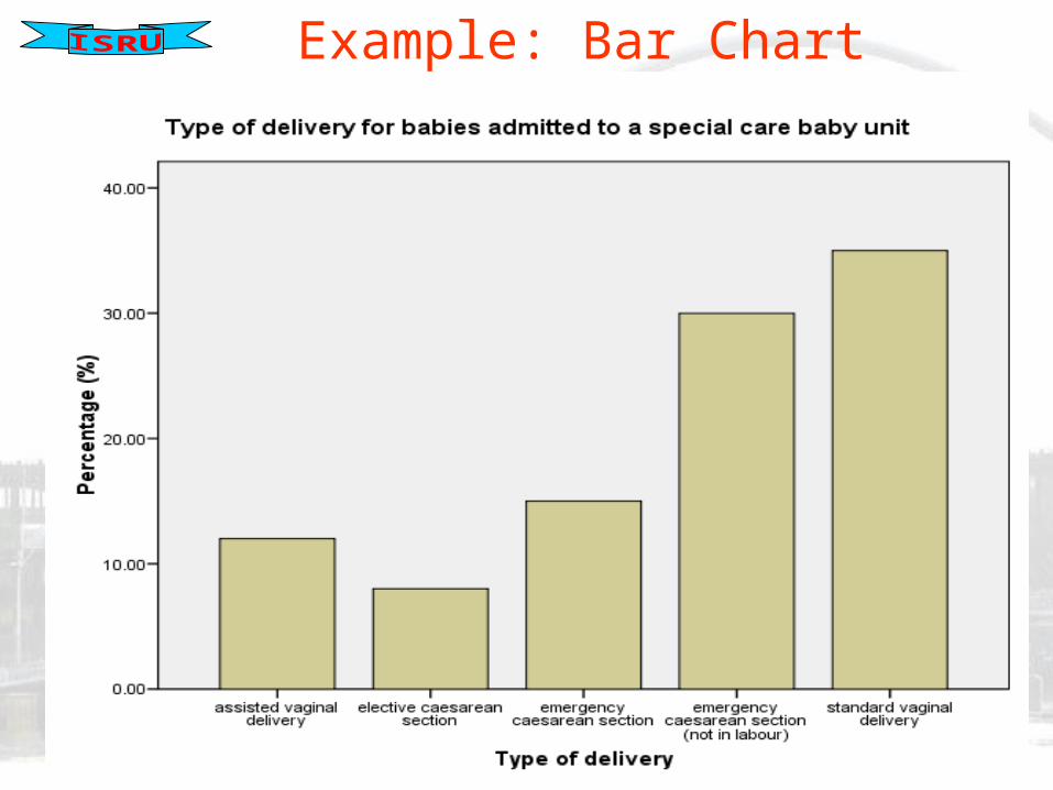
Example: Bar Chart

Pie Chart
A circular ‘pie’ that is split into sections
Each section represents a category
The area of each section is proportional to the frequency in the category

Example: Pie Chart
What could improve this chart?

Box Plot
Sometimes called a ‘Box and Whisker Plot’
A vertical or horizontal rectangle
Ends of the rectangle correspond to the upper and lower quartiles of the data values
A line drawn in the rectangle corresponds to the median value
Whiskers indicate minimum and maximum values but sometimes relate to percentiles (e.g. the 5th and 95th percentile)
Outliers are often marked with an asterix

Example: Box Plot

Histogram
Similar to a bar chart, but no gaps between the bars (the data is continuous)
The width of each bar relates to a range of values for the variable
Area of the bar proportional to the frequency in that range
Usually between 5-20 groups are chosen

Example: Histogram

‘Shape’ of the frequency distribution
The choice of the most appropriate statistical method is often dependent on the shape of the distribution
Shape can be:
– Unimodal – single peak
– Bimodal – Two peaks
– Uniform – no peaks, each value equally likely

Unimodal data
When the distribution is unimodal it’s important to assess where the majority of the data values lie
Is the data:
– Symmetrical (centred around some mid-point)
– Skewed to the right (positively skewed) – long tail to the right
– Skewed to the left (negatively skewed) – long tail to the left

Displaying two variables
If one variable is categorical, separate diagrams showing the distribution of the second variable can be drawn for each of the categories
Clustered or segmented bar charts are also an option
If variables are numerical or ordinal then a scatter plot can be used to display the relationship between the two

Example: Scatter Plot
2520151050
80
70
60
50
40
30
20
10
0
Time on Diet
Weig
ht
Loss
Scatterplot of Weight Loss vs Time on Diet

Fitting the Line
If the scatter plot of y versus x looks approximately linear, how do we decide where to put the line of best fit?
By eye?
A standard procedure for placing the line of best fit is necessary, otherwise the line fitted to the data would change depending on who was examining the data

Regression
The least-squares regression method is used to achieve this
This method minimises the sum of the squared vertical differences between the observed y values and the line i.e. the least-squares regression line minimises the error between the predicted values of y and the actual y values
The total prediction error is less for the least-squares regression line than for any other possible prediction line

Example: Scatter Plot with Regression Line
2520151050
80
70
60
50
40
30
20
10
0
Time on Diet
Weig
ht
Loss
Scatterplot of Weight Loss vs Time on Diet
Weight Loss = 1.69 + 3.47 Time on Diet

Session Summary
Bar Chart
Pie Chart
Box Plot
Histogram
Scatter Plot

Distributions

Motivation
Why important?
– if the empirical data approximates to a particular probability distribution, theoretical knowledge can be used to answer questions about the data
– Note: Empirical distribution is the observed distribution (observed data) of a variable
– the properties of distributions provide the underlying theory in some statistical tests (parametric tests)
– the Normal Distribution is extremely important

Important point
It is not necessary to completely understand the theory behind probability distributions!
It is important to know when and how to use the distributions
Concentrate on familiarity with the basic ideas, terminology and perhaps how to use statistical tables (although statistical software packages have made the latter point less essential)

Normal Distribution
Used as the underlying assumption in many statistical tests
Bell-shaped
Symmetrical about the mean
Flattened as the variance increases (fixed mean)
Peaked as the variance decreases (fixed mean)
Shifted to the right if mean increases
Shifted to the left if mean decreases
Mean and Median of a Normal Distribution are equal


≈ 3 standard deviations (3 )
Intervals of the Normal Distribution
99.7%
95%
68%

Other distributions
t-distribution
distribution
F- distribution
2χ

Sampling and Estimation

Motivation
Why important?
– studying the entire population in the majority of cases is impractical, time consuming and/or resource intensive
– samples are used in studies to estimate characteristics and draw conclusions about the population

Populations and Samples
Population – the entire group of individuals in whom we are interested
E.g.
– All season ticket holders at Newcastle United
– All students at the University of Newcastle upon Tyne
– The entire population of the UK
– All patients with a certain medical condition
Sample – any subset of a population

Sampling
Samples should be ‘representative’ of the population Some degree of sampling error will exist when the
whole population is not used Asking people to choose a ‘representative’ sample is
subjective as people will choose differently. An objective method for selecting the samples is
desirable – a sampling strategy The advantage of sampling strategies are that they
avoid subjectiveness and bias

Sampling Strategies
Include:
Simple Random Sampling (SRS) Systematic Sampling Cluster Sampling Stratified Random Sampling

Simple Random Sampling
Sample chosen so that every member of a
population has the same chance (probability) of being included in the sample
To carryout Simple Random Sampling a list of all the sample units in the population is required (a sampling frame)
Each unit is assigned a number and ‘n’ units are selected from the population
Simple Random Sampling
Advantage SRS is a fairly simple and effective method of
obtaining a random sample from a population
Disadvantages It can theoretically result in an unbalanced sample
that does not truly represent some sector of the population.
It can be an expensive way to sample from a population which is spread out over a large geographic area
Point Estimates
It is often required to estimate the value of a parameter of a population e.g. the mean
Can estimate the value of the population parameter using the data collected in the sample
The estimate is referred to as the point estimate of the parameter as opposed to an interval estimate which takes a range of values

Sampling variation
If repeated samples were taken from a population it is unlikely that the estimates of the population (e.g. estimates of the mean) would be identical in each sample
However, the estimates should all be close to the true value of the population and similar to one other
By quantifying the variability of these estimates, information can be obtained on the precision of the estimate and sampling error can be assessed
In medical studies, usually only one sample is taken from a population, as opposed to many
Have to make use of the knowledge of the theoretical distribution of sample estimates to draw inferences about the population parameter

Sampling distribution of the mean
Many repeated samples of size n from a population can be drawn
If the mean of each sample was calculated a histogram of the means could be drawn; this would show the sampling distribution of the mean
It can be shown that:
– the mean estimates follow a Normal Distribution whatever the distribution of the original data (Central Limit Theorem)
– if the sample size is small, the estimates of the mean follow a Normal Distribution provided the data in the population follow a Normal Distribution
– the mean of the estimates equals the true population mean

Sampling distribution of the mean
– The variability of the distribution is measured by the standard error of the mean (SEM)
– The standard error of the mean is given by:
– where is the population standard deviation and n is the sample size
n
σ SEM
σ

Best estimates in reality
When we have only one sample (as is the usual reality), the best estimate of the population mean is the sample mean and the standard error of the mean is given by:
where s is the standard deviation of the observations in the samples and n is the sample size
n
s SEM

Interpreting standard errors
A large standard error means that the estimate of the population mean is imprecise
A small standard error means that the estimate of the population mean is precise
A more precise estimate of the population mean can be obtained if:
– the size of the sample is increased
– the data is less variable

Using SD or SEM
SD, the standard deviation, is used to describe the variation in the data values
SEM, the standard error of the mean, is used to describe the precision of the sample mean
– should be used if you are interested in the mean of data values

Confidence Intervals

Motivation
Why important?
– used to provide a measure of precision for a population parameter such as the mean
– can be used in statistical tests as a method of testing whether the results are clinically important

Confidence Intervals
The standard error is not by itself particularly useful
It is more useful to incorporate the measure of precision into an interval estimate for the population parameter – this is known as a confidence interval
The confidence interval extends either side of the point estimate by some multiple of the standard error

A 95% Confidence Interval
A 95% confidence interval for the population mean is given by:
If the study were to be repeated many times, this interval would contain the true population mean on 95% of occasions
Usual interpretation: the range of values within which we are 95% confident that the true population lies – although not strictly correct
n
s.xμ
n
s.x
961961

Interpretation of CI intervals
A wide interval indicates that the estimate for the population parameter is imprecise, a narrow one indicates that the estimate is precise
The upper and lower limits provide a means of assessing whether the results of a test are clinically important
Can check whether a hypothesised value for the population parameter falls within the confidence interval

Hypothesis Testing

Motivation
Why important?
– used to quantify a belief against a particular hypothesis (a statistical test is performed)
e.g. the hypothesis is that the rates of cardiovascular disease are the same in men and women in the population
– a statistical test could be conducted to determine the likelihood that this is correct, making a decision based on statistical evidence as to whether the hypothesis should be rejected or not rejected

Hypothesis Testing
Once data is collected a process called Hypothesis Testing is used to analyse it
There are specific types of hypothesis tests
Five general stages for hypothesis testing can be defined:

Stages of Hypothesis Testing
1. Define the Null & Alternative Hypotheses under study
2. Collect data
3. Calculate the value of the test statistic
4. Compare the value of the test statistic to values from a known probability distribution
5. Interpret the P-value and results

The Null Hypothesis
The Null Hypothesis is tested which assumes no effect (e.g. the difference in means equals zero) in the population
E.g. Comparing the rates of cardiovascular disease in men and woman in the population
Null Hypothesis H0: rates of cardiovascular disease are the same in men and woman in the population

The Alternative Hypothesis
The Alternative Hypothesis is then defined, this holds if the Null Hypothesis is not true
E.g. Alternative Hypothesis H1: rates of cardiovascular disease are different in men and woman in the population

Two-tail testing
In the previous example no direction for the difference in rates was specified
i.e. it was not stated whether men have higher or lower rates than woman
A two-tailed test is often recommended because the direction is rarely certain in advance, if one does exist
There are circumstance in which a one-tailed test is relevant

The test statistic
After data collection, the sample values are substituted into a formula, specific to the type of hypothesis test
A test statistic is calculated
The test statistic is effectively the amount of evidence in the data against H0
The larger the value (irrelevant of sign), the greater the evidence
Test statistics follow known theoretical probability distributions

The P-value
The test statistic is compared to values from a known probability distribution to obtain the P-value
The P-value is the area in both tails (occasionally one) of the probability distribution
The P-value is the probability of obtaining our results, or something more extreme, if the Null Hypothesis is true
The Null Hypothesis relates to the population rather than the sample

Use of the P-value
A decision must be made as to how much evidence is required to reject H0 in favour of H1
The smaller the P-value, the greater the evidence against H0

Conventional use of the P-value – rejecting H0
Conventionally, if the P-value < 0.05, there is sufficient evidence to reject H0
There is only a small chance of the results occurring if H0 is true
– H0 is rejected, the results are significant at the 5% level
Conventional use of the P-value – not rejecting H0
If the P-value > 0.05, there is insufficient evidence to reject H0
– H0 is not rejected, the results are not significant at the 5% level
NB: This does not mean that the null hypothesis is true, simply that we do not have enough evidence to reject it!

Using 5%
The choice of 5% is arbitrary, on 5% of occasions H0 will be incorrectly rejected when it is true (Type I error)
In some clinical situations stronger evidence may be required before rejecting H0
– e.g. rejecting H0 if the P-value is less than 1% or 0.1%
The chosen cut-off for the P-value is called the significance level of the test; it must be chosen before the data is collected

Parametric vs. Non-Parametric Tests
Hypothesis Tests which are based on knowledge of the probability distribution that the data follow are known as parametric tests
Often data does not conform to the assumptions that underly these methods
In these cases non-parametric tests are used
Non-Parametric Tests make no assumption about the probability distribution and generally replace the data with their ranks

Non-parametric tests
Useful when:
• sample size is small
• data is measured on a categorical scale (though can be used on numerical data as well)
However:
• they have less power of detecting a real difference than the equivalent parametric tests if all the assumptions underlying the parametric test are true
• they lead to decisions rather than generating a true understanding of the data

Statistical tests
Quantitative data, Parametric tests
– One-sample t-test
– Two-sample t-test
– Paired t-test
– One-way ANOVA

Statistical tests
Quantitative data, Non-parametric tests
– Sign test
– Wilcoxon signed ranks test
– Mann-Whitney U test
– Kruskal-Wallis test

Statistical tests
Qualitative data, Non-parametric tests
– z-test for a proportion
– McNemar’s test
– Chi-squared test
– Fisher’s exact test

Choosing a statistical test
Useful medical statistical books will contain a flowchart to help decide on the correct statistical test
Considerations include:
– Is the data quantitative or qualitative?
– How many groups of data are there?
– Can a probability distribution be assumed?

Examples

Paired t-test

Two sample t-test (paired)
Two samples related to each other and one numerical or ordinal variable of interest
E.g. in a cross-over trial, each patient has two measurements on the variable, one while taking treatment, one while taking a placebo
E.g. the individuals in each sample may be different but linked to each other in some way

Assumptions
The individual differences are Normally distributed with a given variance
A reasonable sample size has been taken so that the assumption of Normality can be checked

Assumptions not satisfied
If the differences do not follow a Normal distribution, the assumption underlying the t-test is not satisfied
Options:
– Transform the data
– Use a non-parametric test such as the Sign Test or Wilcoxon signed ranks test
Example
A peak expiratory flow rate (PEFR) was taken from a random sample of 9 asthmatics before and after a walk on a cold day
The mean of the differences before and after the walk = 56.11
The standard deviation of the differences = 34.17
Does the walk significantly influence the PEFR?
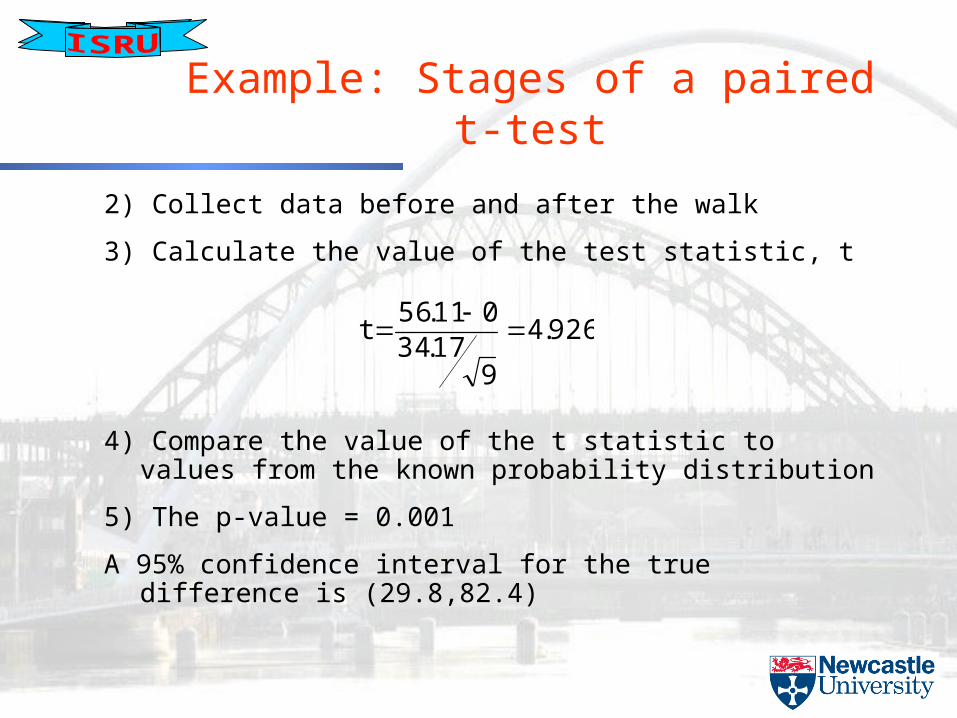
Example: Stages of a paired t-test
1) Define the Null and Alternative hypotheses under study:
Ho: the mean difference = 0
H1: the mean difference ≠ 0
Example: Stages of a paired t-test
2) Collect data before and after the walk
3) Calculate the value of the test statistic, t
4) Compare the value of the t statistic to values from the known probability distribution
5) The p-value = 0.001
A 95% confidence interval for the true difference is (29.8,82.4)
xt
926.4
917.34
011.56t

Paired t-test results
– there is strong evidence to reject the Null Hypothesis in favour of the Alternative Hypothesis
– there is strong evidence that the walk significantly effects PEFR, the difference ≠ 0
Paired Samples Statistics
323.8889 9 59.82567 19.94189
267.7778 9 50.00694 16.66898
Before Walk
After walk
Pair1
Mean N Std. DeviationStd. Error
Mean
Paired Samples Test
56.11111 34.17398 11.39133 29.84266 82.37956 4.926 8 .001Before Walk - After walkPair 1Mean Std. Deviation
Std. ErrorMean Lower Upper
95% ConfidenceInterval of the
Difference
Paired Differences
t df Sig. (2-tailed)

Mann-Whitney test

Mann-Whitney U test
The Mann-Whitney U test – two independent samples test
It is equivalent to the Kruskal-Wallis test for two groups
Mann-Whitney tests that two sampled populations are equivalent in location

Methodology
The observations from both groups are combined and ranked, with the average rank assigned in the case of ties
If the populations are identical in location, the ranks should be randomly mixed between the two samples
The test calculates the number of times that a score from group 1 precedes a score from group 2 and the number of times that a score from group 2 precedes a score from group 1
Example
Two samples of diastolic blood pressure were taken
Is there a difference in the population locations without assuming a parametric model for the distributions?
The equality of population means is tested through the use of a Mann-Whitney test
Are the two populations significantly different?

Example - Mann-Whitney U test
Ranks
8 7.50 60.00
9 10.33 93.00
17
Group1.00
2.00
Total
Diastolic BloodPressure 1
N Mean Rank Sum of Ranks
Test Statisticsb
24.000
60.000
-1.156
.248
.277a
Mann-Whitney U
Wilcoxon W
Z
Asymp. Sig. (2-tailed)
Exact Sig. [2*(1-tailedSig.)]
DiastolicBlood
Pressure 1
Not corrected for ties.a.
Grouping Variable: Groupb.
- there is no evidence to reject the Null Hypothesis in favour of the Alternative Hypothesis, p-value = 0.277 >0.05
- there is no evidence of a difference in blood pressure medians

Errors in Hypothesis Testing

Motivation
Why important?
– when interpreting the results of a statistical test, there is always a probability of making an erroneous conclusion (however minimal)
– it is important to ensure that these probabilities are minimised
– possible mistakes are called Type I and Type II errors

Type I error
Rejecting the Null Hypothesis when it is true
Concluding that there is an effect when in reality there is none
The maximum chance of making a Type I error is denoted by alpha α
α is the significance level of the test, we reject the null hypothesis if the p-value is less than the significance level

Type II error
Not rejecting the Null Hypothesis when it is false
Concluding that there is no effect when one really exists
The chance of making a Type II error is denoted by beta β
Its compliment 1- β, is the power of the test

Power of the test
The Power is the probability of rejecting the Null Hypothesis when it is false
i.e. the probability of making a correct decision
The ideal power of the test is 100%
However there is always a possibility of making a Type II error

Sample Size

Motivation
Why important?
– if the sample size is too small, there may be inadequate test power to detect an important existing effect/difference and resources will be wasted
– if the sample size is too large, the study may be unnecessarily time consuming, expensive and unethical
– have to determine a sample size which strikes a balance between making a Type I or Type II error
– an optimal sample size can be difficult to establish as an estimate of the results expected in the study is required

Calculating an optimal sample size for a test
The following quantities need to be specified at the design stage of the investigation in order to calculate an optimal sample size:
– The Power
– Significance level
– Variability
– Smallest effect of interest

Summary
Data Types
Descriptive Statistics
Graphical Summaries
Distributions
Sampling and Estimation
Confidence Intervals
Hypothesis Testing (Statistical tests)
Errors in Hypothesis Testing
Sample Size

Book Reference
Medical Statistics at a Glance, 3rd Edition
(Aviva Petrie & Caroline Sabin)
ISBN: 978-1-4051-8051-1