Basic Statistics I

Biostatistics, MHA, CDC, Jul 09

Prof. K.G. Satheesh Kumar

Asian School of Business

What and why!

Statistics* is a discipline that deals with:• collection of data;• their classification and summarising;• analysis

for drawing conclusions and making decisions* Statistics also refers to the data obtained from sample (as against parameter for

population data)

Analysis provides us an understanding of the variation# and its causes in a phenomenon

# World is full of variations that it is hard to tell real differences from natural variations

Descriptive & Inferential Statistics

• Descriptive Statistics is concerned with organisation, summarisation and presentation of data

• Inferential Statistics deals with drawing conclusions about large groups of subjects (population) on the basis of observations obtained from some of them (sample)

Variables

• A variable is what is being observed or measured

• Gender, age, height, weight, colour of eye, responsiveness to treatment, life expectancy, preferences etc. are examples

• Dependent variable is an outcome of interest that changes in response to some intervention

• Independent variable is the intervention, or what is being manipulated (sometimes without manipulation e.g. age)

Types of Data

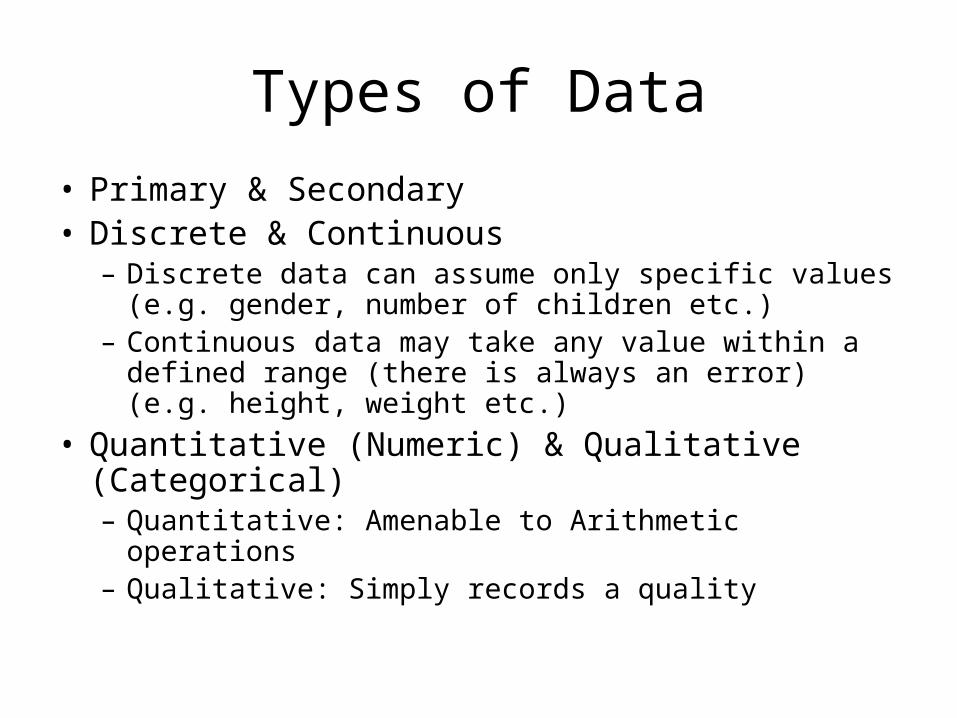
• Primary & Secondary• Discrete & Continuous

– Discrete data can assume only specific values (e.g. gender, number of children etc.)

– Continuous data may take any value within a defined range (there is always an error) (e.g. height, weight etc.)

• Quantitative (Numeric) & Qualitative (Categorical)– Quantitative: Amenable to Arithmetic operations– Qualitative: Simply records a quality

Types of Data (Contd…)

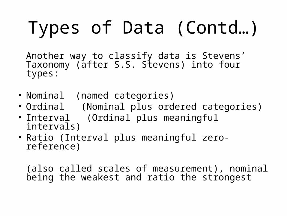
Another way to classify data is Stevens’ Taxonomy (after S.S. Stevens) into four types:

• Nominal (named categories)• Ordinal (Nominal plus ordered categories)• Interval (Ordinal plus meaningful intervals)• Ratio (Interval plus meaningful zero-reference)

(also called scales of measurement), nominal being the weakest and ratio the strongest

Nominal Variable

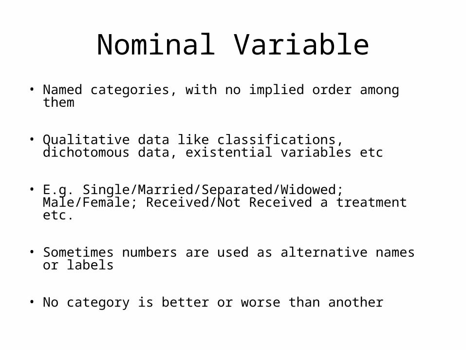
• Named categories, with no implied order among them

• Qualitative data like classifications, dichotomous data, existential variables etc

• E.g. Single/Married/Separated/Widowed; Male/Female; Received/Not Received a treatment etc.

• Sometimes numbers are used as alternative names or labels

• No category is better or worse than another

Ordinal Variable

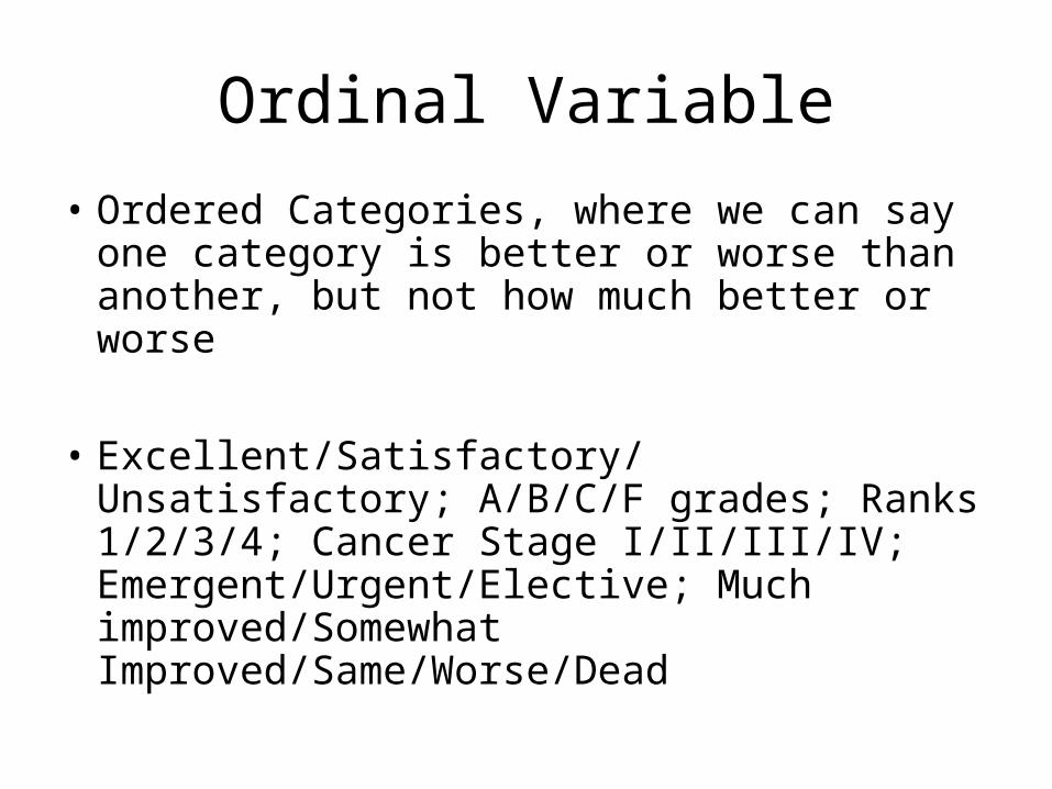
• Ordered Categories, where we can say one category is better or worse than another, but not how much better or worse

• Excellent/Satisfactory/Unsatisfactory; A/B/C/F grades; Ranks 1/2/3/4; Cancer Stage I/II/III/IV; Emergent/Urgent/Elective; Much improved/Somewhat Improved/Same/Worse/Dead

Interval Variable

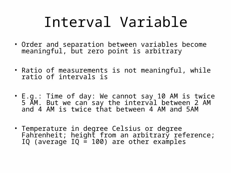
• Order and separation between variables become meaningful, but zero point is arbitrary

• Ratio of measurements is not meaningful, while ratio of intervals is

• E.g.: Time of day: We cannot say 10 AM is twice 5 AM. But we can say the interval between 2 AM and 4 AM is twice that between 4 AM and 5AM

• Temperature in degree Celsius or degree Fahrenheit; height from an arbitrary reference; IQ (average IQ = 100) are other examples

Ratio Variable

• If the zero point is meaningful, the ratio between two measurements is also meaningful – such variables are ratio variables

• Lengths, weights, money, absolute temperature, duration (not time of day), volume, area etc. are examples

Describing Data

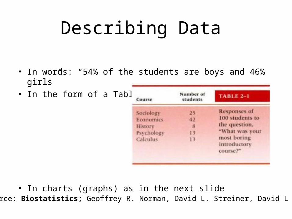
• In words: “54% of the students are boys and 46% girls”• In the form of a Table*

• In charts (graphs) as in the next slide* Source: Biostatistics; Geoffrey R. Norman, David L. Streiner, David L Streiner

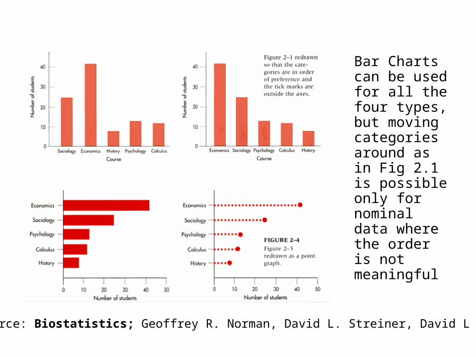
Bar Charts can be used for all the four types, but moving categories around as in Fig 2.1 is possible only for nominal data where the order is not meaningful

* Source: Biostatistics; Geoffrey R. Norman, David L. Streiner, David L Streiner

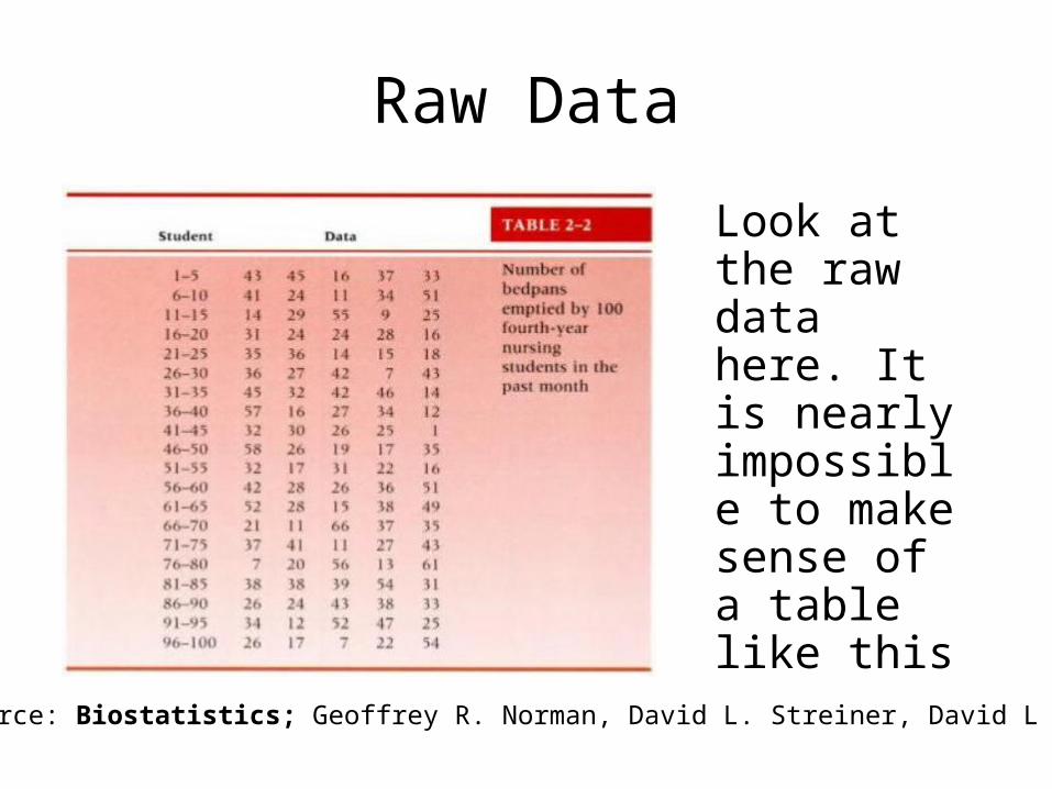
Raw Data

Look at the raw data here. It is nearly impossible to make sense of a table like this

* Source: Biostatistics; Geoffrey R. Norman, David L. Streiner, David L Streiner

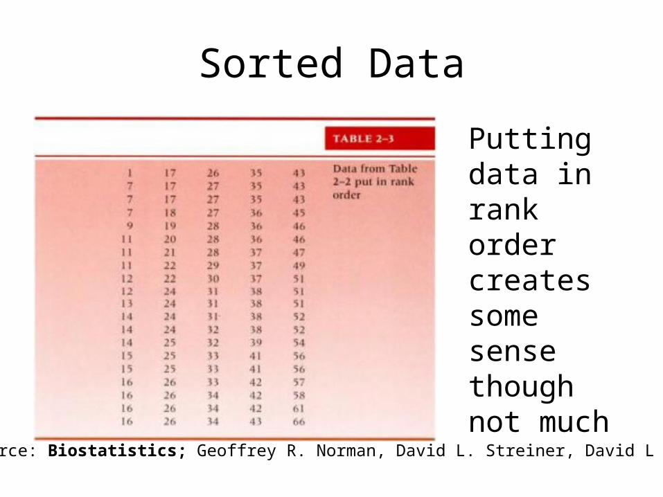
Sorted Data

Putting data in rank order creates some sense though not much

* Source: Biostatistics; Geoffrey R. Norman, David L. Streiner, David L Streiner

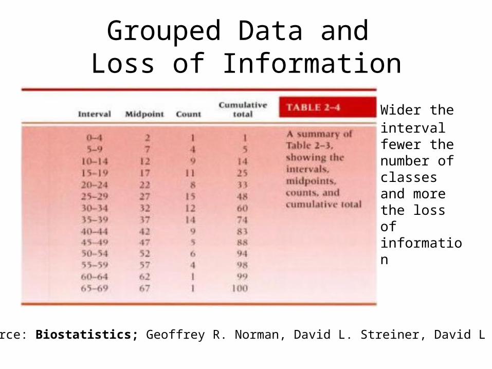
Grouped Data and Loss of Information

Wider the interval fewer the number of classes and more the loss of information

* Source: Biostatistics; Geoffrey R. Norman, David L. Streiner, David L Streiner

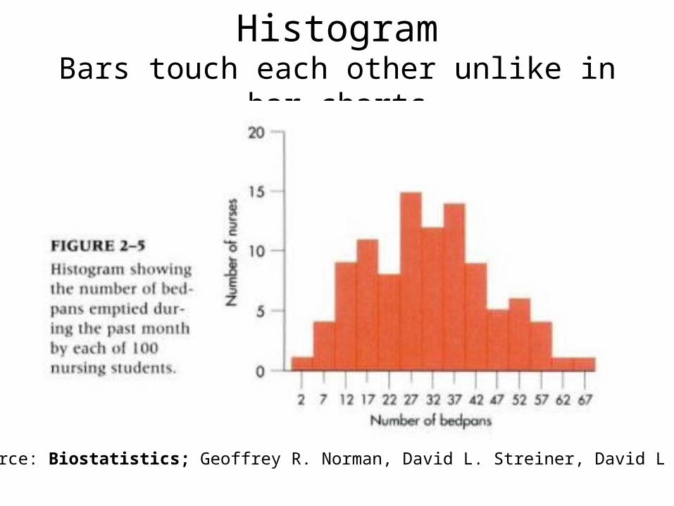
HistogramBars touch each other unlike in bar charts

* Source: Biostatistics; Geoffrey R. Norman, David L. Streiner, David L Streiner

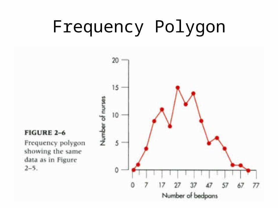
Frequency Polygon

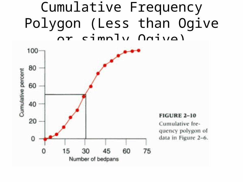
Cumulative Frequency Polygon (Less than Ogive or simply Ogive)

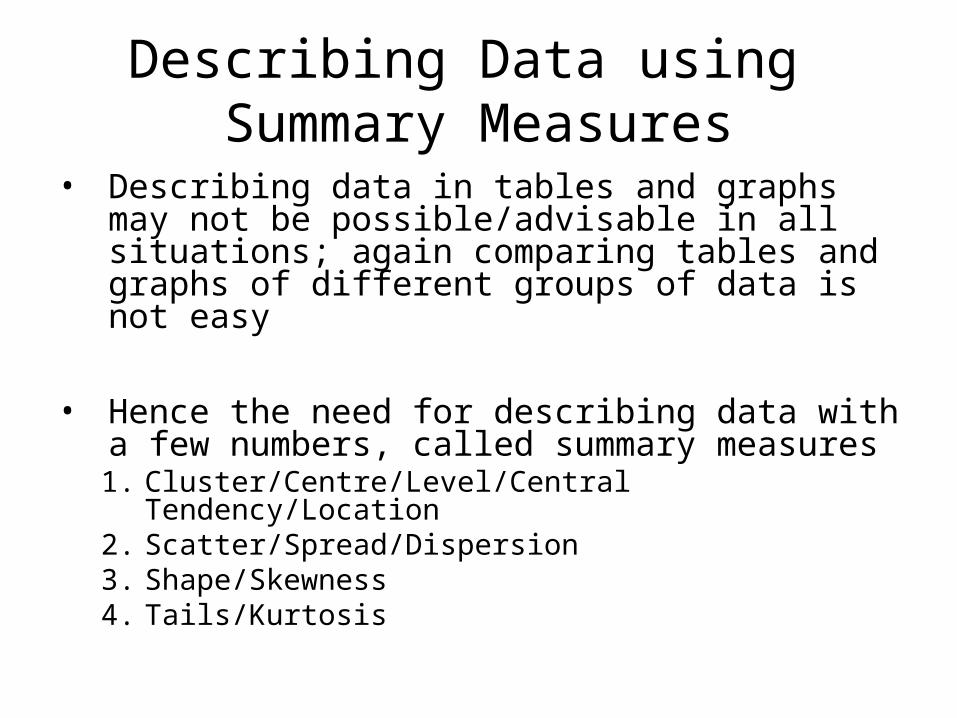
Describing Data using Summary Measures

• Describing data in tables and graphs may not be possible/advisable in all situations; again comparing tables and graphs of different groups of data is not easy

• Hence the need for describing data with a few numbers, called summary measures1. Cluster/Centre/Level/Central Tendency/Location2. Scatter/Spread/Dispersion3. Shape/Skewness4. Tails/Kurtosis

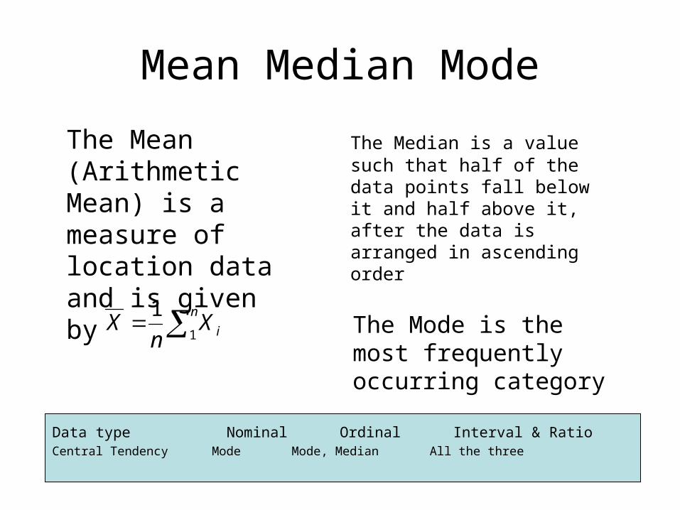
Mean Median Mode

The Mean (Arithmetic Mean) is a measure of location data and is given by

n

iXnX

1

1

The Median is a value such that half of the data points fall below it and half above it, after the data is arranged in ascending order

The Mode is the most frequently occurring category

Data type Nominal Ordinal Interval & RatioCentral Tendency Mode Mode, Median All the three

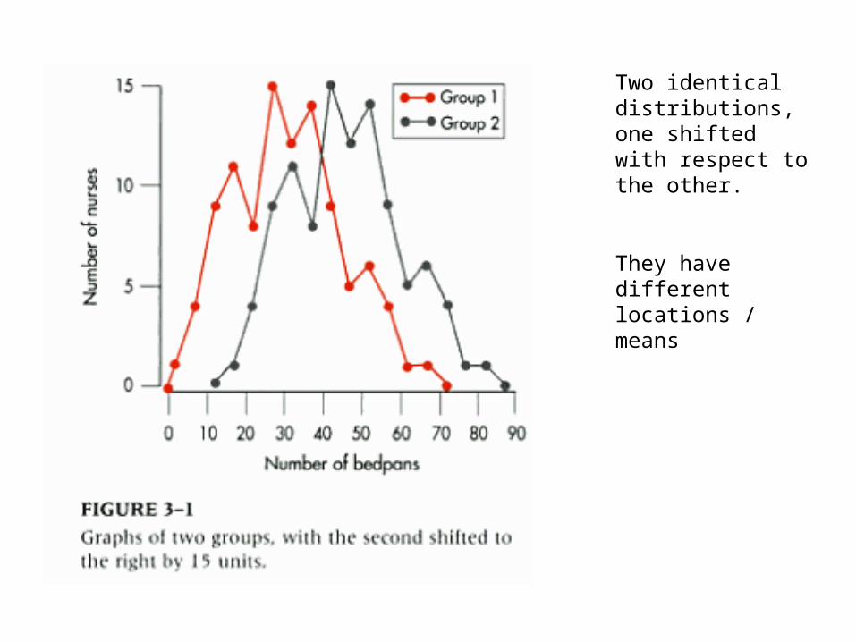
Two identical distributions, one shifted with respect to the other.

They have different locations / means

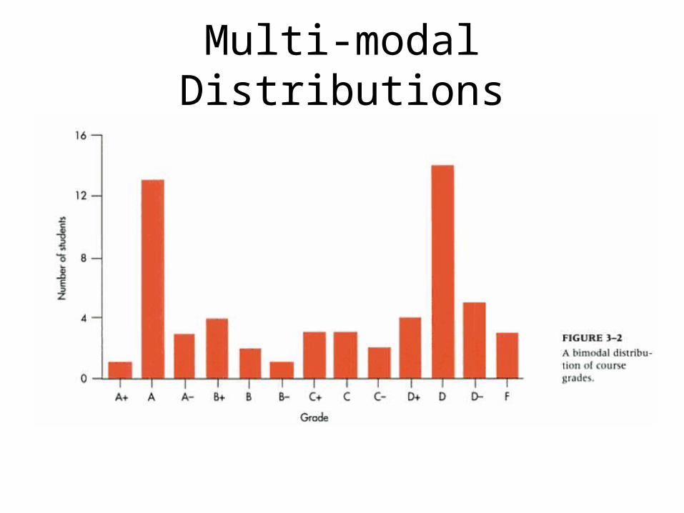
Multi-modal Distributions

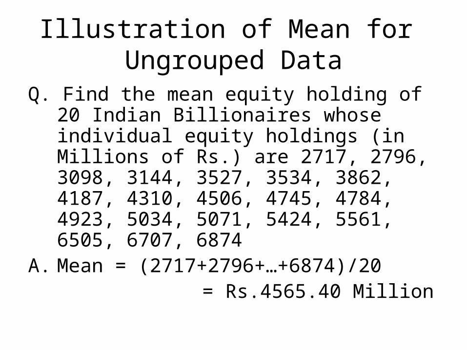
Illustration of Mean for Ungrouped Data

Q. Find the mean equity holding of 20 Indian Billionaires whose individual equity holdings (in Millions of Rs.) are 2717, 2796, 3098, 3144, 3527, 3534, 3862, 4187, 4310, 4506, 4745, 4784, 4923, 5034, 5071, 5424, 5561, 6505, 6707, 6874

A. Mean = (2717+2796+…+6874)/20 = Rs.4565.40 Million

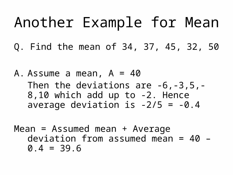
Another Example for Mean

Q. Find the mean of 34, 37, 45, 32, 50

A. Assume a mean, A = 40Then the deviations are -6,-3,5,-8,10 which add up to -2. Hence average deviation is -2/5 = -0.4

Mean = Assumed mean + Average deviation from assumed mean = 40 – 0.4 = 39.6

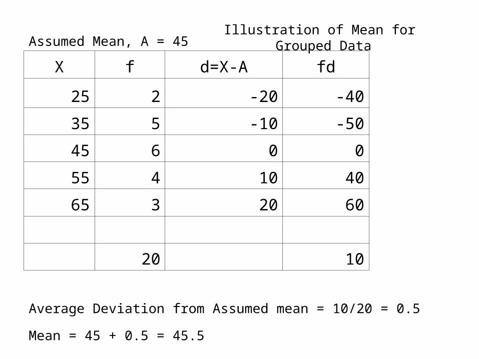
Illustration of Mean for Grouped DataAssumed Mean, A = 45

X f d=X-A fd

25 2 -20 -40

35 5 -10 -50

45 6 0 0

55 4 10 40

65 3 20 60

       

  20   10

Average Deviation from Assumed mean = 10/20 = 0.5

Mean = 45 + 0.5 = 45.5

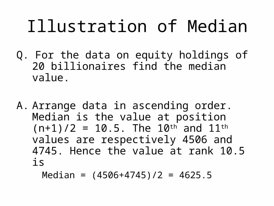
Illustration of Median

Q. For the data on equity holdings of 20 billionaires find the median value.

A. Arrange data in ascending order. Median is the value at position (n+1)/2 = 10.5. The 10th and 11th values are respectively 4506 and 4745. Hence the value at rank 10.5 is

Median = (4506+4745)/2 = 4625.5

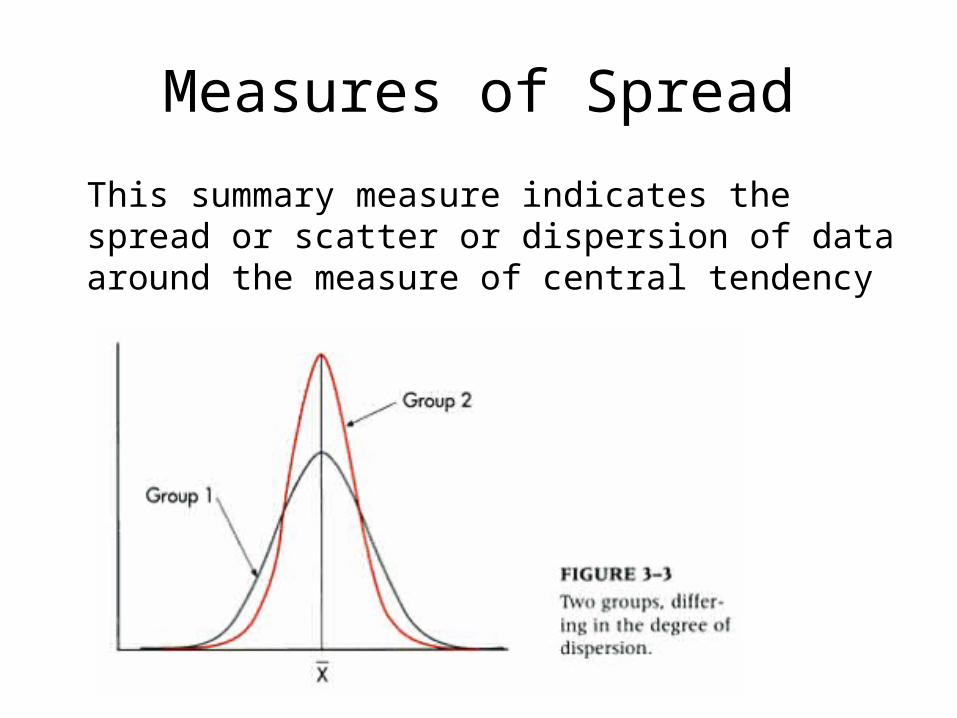
Measures of Spread

This summary measure indicates the spread or scatter or dispersion of data around the measure of central tendency

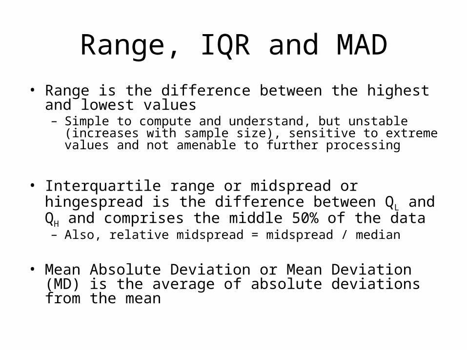
Range, IQR and MAD

• Range is the difference between the highest and lowest values– Simple to compute and understand, but unstable (increases with

sample size), sensitive to extreme values and not amenable to further processing

• Interquartile range or midspread or hingespread is the difference between QL and QH and comprises the middle 50% of the data– Also, relative midspread = midspread / median

• Mean Absolute Deviation or Mean Deviation (MD) is the average of absolute deviations from the mean

Quartiles

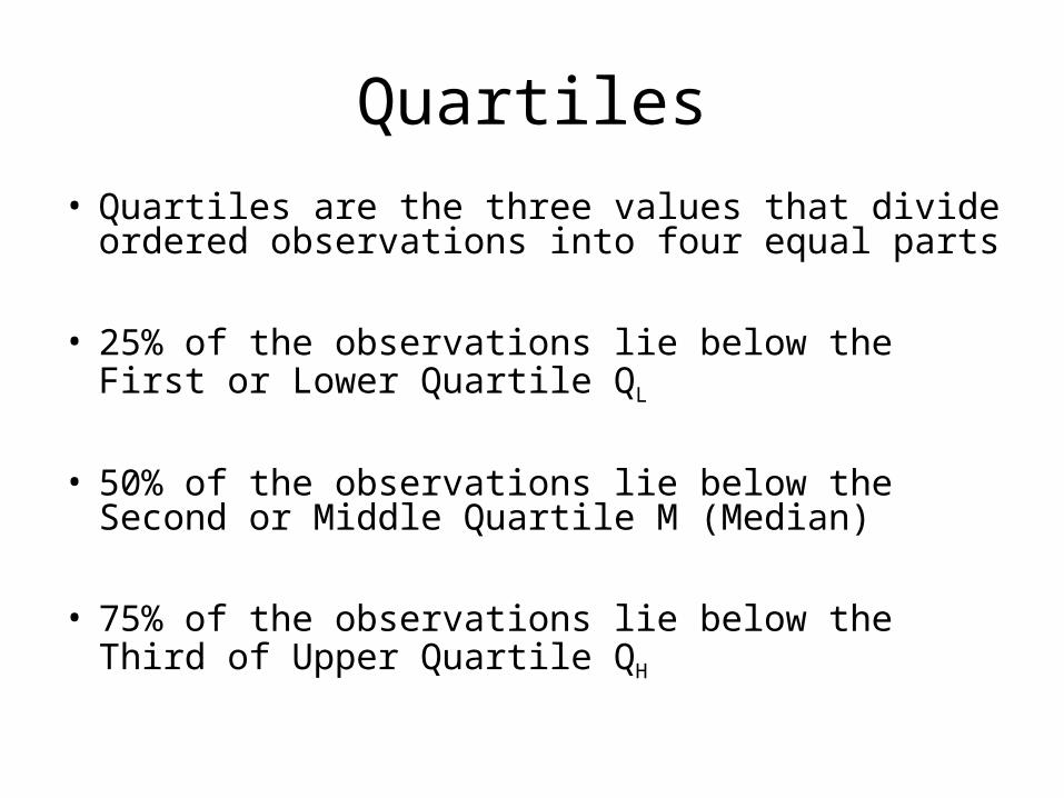
• Quartiles are the three values that divide ordered observations into four equal parts

• 25% of the observations lie below the First or Lower Quartile QL

• 50% of the observations lie below the Second or Middle Quartile M (Median)

• 75% of the observations lie below the Third of Upper Quartile QH

Illustration

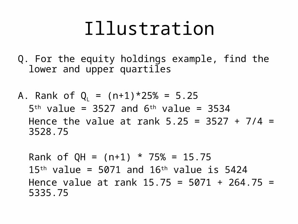
Q. For the equity holdings example, find the lower and upper quartiles

A. Rank of QL = (n+1)*25% = 5.255th value = 3527 and 6th value = 3534 Hence the value at rank 5.25 = 3527 + 7/4 = 3528.75

Rank of QH = (n+1) * 75% = 15.7515th value = 5071 and 16th value is 5424Hence value at rank 15.75 = 5071 + 264.75 = 5335.75

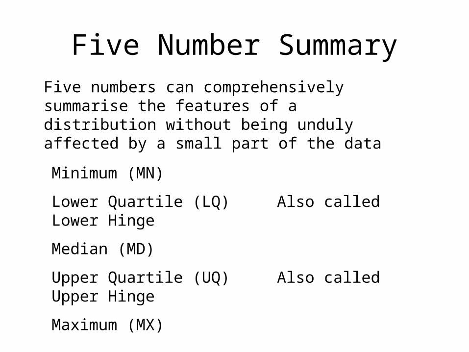
Five Number SummaryFive numbers can comprehensively summarise the features of a distribution without being unduly affected by a small part of the data

Minimum (MN)

Lower Quartile (LQ) Also called Lower Hinge

Median (MD)

Upper Quartile (UQ) Also called Upper Hinge

Maximum (MX)

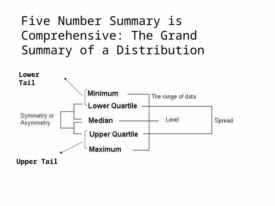
Lower Tail

Upper Tail

Five Number Summary is Comprehensive: The Grand Summary of a Distribution

Variance and Standard Deviation

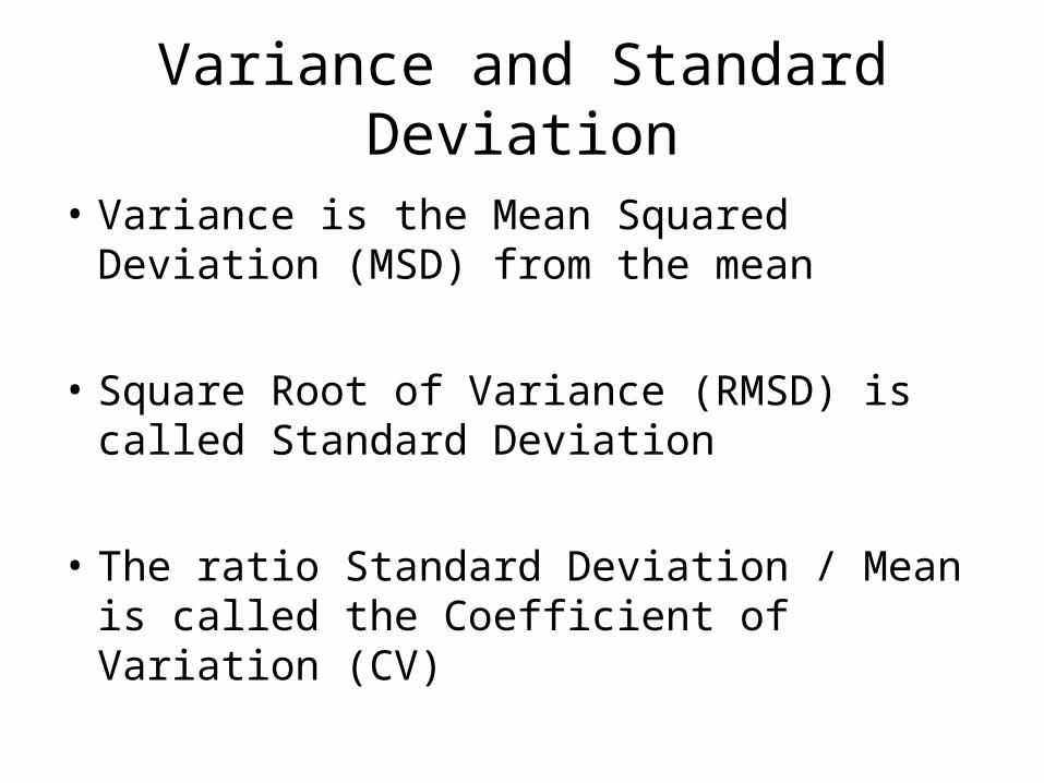
• Variance is the Mean Squared Deviation (MSD) from the mean

• Square Root of Variance (RMSD) is called Standard Deviation

• The ratio Standard Deviation / Mean is called the Coefficient of Variation (CV)

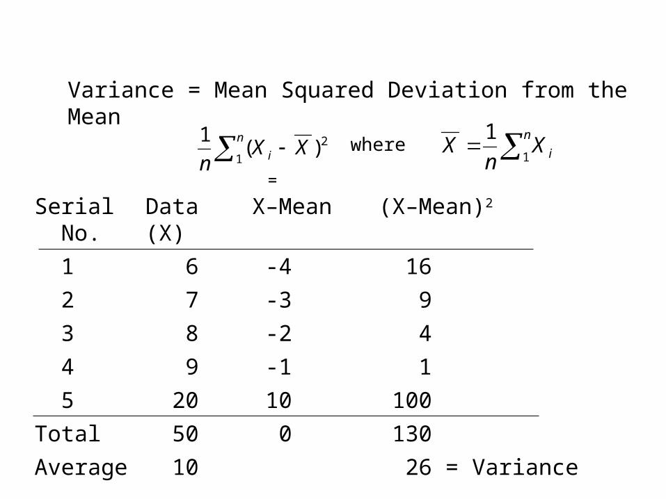
Variance = Mean Squared Deviation from the Mean

= n

i XXn 1

2)(1

Serial No.

Data (X)

X–Mean (X–Mean)2

1 6 -4 16

2 7 -3 9

3 8 -2 4

4 9 -1 1

5 20 10 100

Total 50 0 130

Average 10 26 = Variance

n

iXnX

1

1where

Covariance

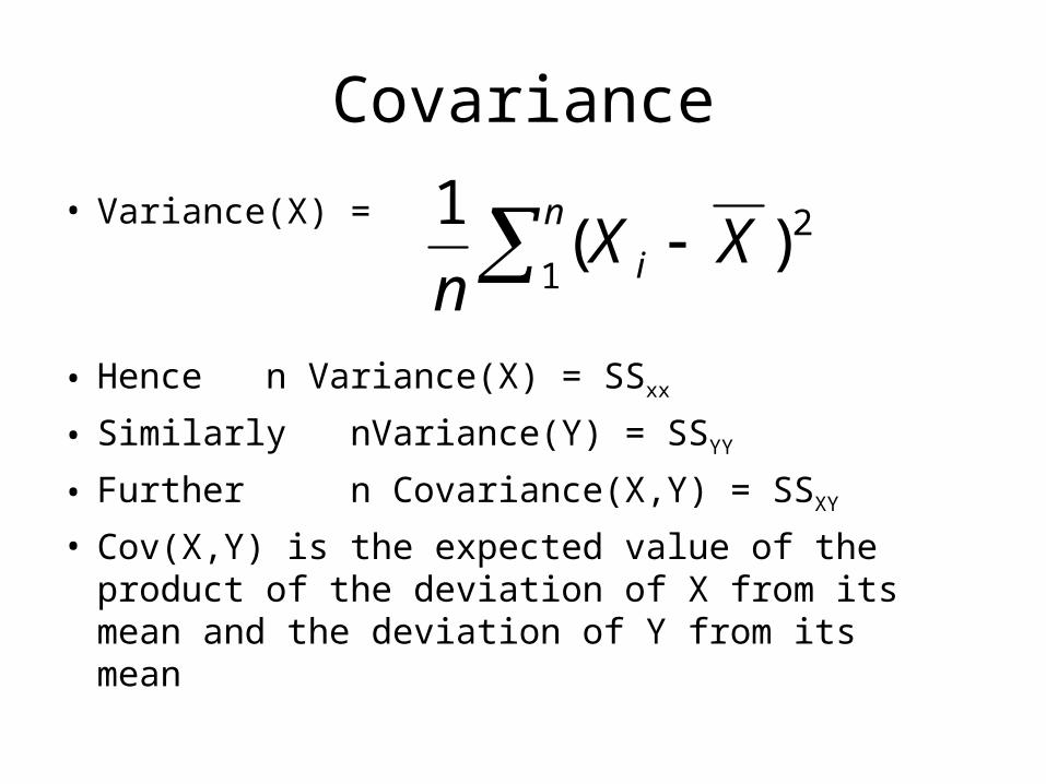
• Variance(X) =

• Hence n Variance(X) = SSxx

• Similarly nVariance(Y) = SSYY

• Further n Covariance(X,Y) = SSXY

• Cov(X,Y) is the expected value of the product of the deviation of X from its mean and the deviation of Y from its mean

n

i XXn 1

2)(1

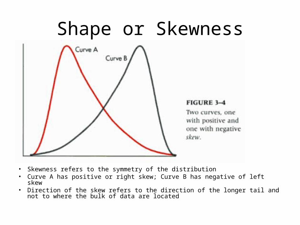
Shape or Skewness

• Skewness refers to the symmetry of the distribution• Curve A has positive or right skew; Curve B has negative of left skew• Direction of the skew refers to the direction of the longer tail and not to

where the bulk of data are located

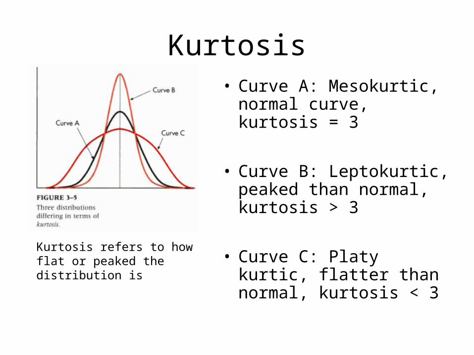
Kurtosis• Curve A: Mesokurtic,

normal curve, kurtosis = 3

• Curve B: Leptokurtic, peaked than normal, kurtosis > 3

• Curve C: Platy kurtic, flatter than normal, kurtosis < 3

Kurtosis refers to how flat or peaked the distribution is

Continued…