basic transformations in 3d - unam · basic geometric transformations in 2d and 3d a tutorial jorge...
TRANSCRIPT
Basic Geometric Transformations in 2D and 3D A Tutorial
Jorge Alberto Márquez Flores, PhD Image Analysis and Visualization Laboratory, CCADET-UNAM, 2012
1. Homogeneous Coordinates. To understand the matrix formulation of 2D and 3D transformations, we justify in this section the practice of using homogeneous coordinates. We first note that a common transformation T in 2D consists of a system of two simultaneous equations:
{: u a x b y cv d x e y f
= + += + +
T (1)
If c = f = 0, T is a linear transformation on (x, y); otherwise, we cannot write a matrix T to transform (x, y) into (u, v) if a non-zero translation (c, f) exists. This because, in able to use Linear Algebra, equation (1) must be a linear transformation, that is, T(x1+x2, y1+y2) should be equal to (T(x1, y1) + T(x2+y2)) and T(αx, αy) = αT(x, y), but (1) does not satisfy in general such conditions: it is not a linear transformation. To “linearize” T we observe that a matrix-product formulation is possible, by stepping up to 3D, if we add a third “idle” equation, “1 = 1”, as follows:
1 1 1 0 0 1 1
u ax b y c u a b c xv d x e y f v c d f y
= + +⎧ ⎛ ⎞ ⎛ ⎞⎛ ⎞⎪ ⎜ ⎟ ⎜ ⎟⎜ ⎟= + + ⇒ =⎨ ⎜ ⎟ ⎜ ⎟⎜ ⎟⎪ =⎩ ⎝ ⎠ ⎝ ⎠⎝ ⎠ (2)
Equations (2) and (1) are equivalent, but a linear formulation in a higher dimension (albeit, consisting of a fixed constant “1”) is obtained: U=TX, enabling the use of Linear Algebra. A similar approach is used for 3D transformations to write column vectors [u v w 1]T=T3D[x y z 1]T. Such extended coordinates are called homogeneous coordinates and also constitute a particular case of a quaternion formulation, where quaternions are an extension of complex numbers to complex 2D vectors. Remember that a complex product is isomorphic to a rotation. Quaternion formulation is an alternative way for deducing the 3D-to-4D extension of equation (2). The tautological, idle or dummy equation “1=1” has a similar role as multiplying a complex quotient by a “special 1”: both numerator and denominator are multiplied by the complex conjugate of the denominator, (thus having a dummy product by a factor 1, and allowing to separate into real and imaginary terms), or when adding a constant “0 = (+a – a)” to complete an expression where a is the missing piece, and making evident some kind of offset equal to –a. Equation (2) is often generalized by introducing the idle equation “k = k”, with k ≠ 0 instead of “1 = 1”. This allows introducing a normalization factor for homogeneous
Basic Transformations in 2D and 3D 2
Computer Graphics - Tutorial by Jorge Marquez - CCADET UNAM 2011
coordinates, in order to have, at the end, the form (x/k, y/k, z/k, 1), with k ≠ 0. See elsewhere the topic of Perspective, where such k becomes a useful device. Without homogeneous coordinates, a matrix approach requires to separate the translation component, to write: [u v w]T = T[x y z]T − [x0 y0 z0]T. *A Note on Extrinsic and Intrinsic Differences, and Invariance
A common concern when comparing two sets of points or objects is to distinguish differences consisting in deformations, orientation, etc, from (natural) differences in shape. The first kind of differences is part of what is called extrinsic differences, and also includes: noise or degradation in general, deformations, computer representation and data acquisition parameters, such as resolution, dynamic range, etc. They also depend on the coordinate system, hence, on position and orientation. The second kind is called intrinsic differences and do not depend on acquisition, orientation, representation, etc., that is, they do not depend on factors external to the objects. Thus, a particular (morphological) feature can be invariant to rotations, and other transformations. Volume, for example is a measure invariant to differences in position, but not invariant to scaling, and such transformation should be compensated, that is, unwarped. The identification and elimination of extrinsic differences is required when comparing two or more objects or data sets. A first step for such elimination is to make corresponding features to match in space, that is, to align both objects and to make their corresponding point representations have coordinates in the same coordinate system. Besides alignment for analysis, geometric transformations are widely used in Computer Graphics and Virtual Reality. Note 1: A non-linear deformation or distortion can be seen as extrinsic or intrinsic. It is extrinsic when it was caused somehow, and intrinsic, when it comes from natural variation. Some authors refer in the first case as distortion, and deformation to the second. It also may combine both, extrinsic and intrinsic components, and they may be difficult to separate. Non-linear deformations are best studied and applied when basic alignment is achieved (that is, when most important extrinsic differences have been eliminated) and they are treated in another tutorial. In the following we will use the convention of the right-handed system of coordinates, with axis lines x, y, z oriented as shown by the arrows in figure 1. A mnemonic for an orientation choice is the right-hand rule: form the orthogonal axis with the right hand with the thumb being axis x, the index corresponding to axis y and the middle finger pointing orthogonally to both, towards the direction of axis z. The orientation of rotations is chosen to be the same for each coordinate axis as anti-clockwise or counterclockwise as watching along that axis towards the origin. This is illustrated in figure 1 for axis Z. The sign convention may however change according to applications and disciplines.
Basic Transformations in 2D and 3D 3
Computer Graphics - Tutorial by Jorge Marquez - CCADET UNAM 2011
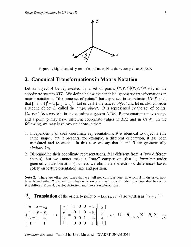
Figure 1. Right-handed system of coordinates. Note the vector product Z=X×Y.
2. Canonical Transformations in Matrix Notation
Let an object A be represented by a set of points{ }( , , )|( , , )x y z x y z A∈ , in the coordinate system XYZ. We define below the canonical geometric transformations in matrix notation as “the same set of points”, but expressed in coordinates UVW, such that [u v w 1]T = T [x y z 1]T. Let us call A the source object and let us also consider a second object B, called the target object. B is represented by the set of points: { }( , , )|( , , )u v w u v w B∈ , in the coordinate system UVW. Representations may change and a point p may have different coordinate values in XYZ and in UVW. In the following, we may have two situations, either: 1. Independently of their coordinate representations, B is identical to object A (the
same shape), but it presents, for example, a different orientation, it has been translated and re-scaled. In this case we say that A and B are geometrically similar. Or,
2. Disregarding their coordinate representations, B is different from A (two different shapes), but we cannot make a “pure” comparison (that is, invariant under geometric transformations), unless we eliminate the extrinsic differences based solely on feature orientation, size and position.
Note 2: There are other two cases that we will not consider here, in which A is distorted non-linearly and either B is equal to A plus distortion plus linear transformations, as described below, or B is different from A, besides distortion and linear transformations.
0pT Translation of the origin to point p0 = (x0, y0, z0) (also written as [x0 y0 z0]T):
0 0 0 0, ,
0 0
0 0
0 0
1 0 00 1 0 ,0 0 1
1 11 1 0 0 0 1
x y z
u x x xu xv y y yv y orw zw z z z
= − −⎡ ⎤⎧ ⎡ ⎤ ⎡ ⎤⎢ ⎥⎪ ⎢ ⎥ ⎢ ⎥= − −⎪ → = ⎢ ⎥⎨ ⎢ ⎥ ⎢ ⎥= − −⎢ ⎥⎪ ⎢ ⎥ ⎢ ⎥
= ⎢ ⎥⎣ ⎦ ⎣ ⎦⎪⎩ ⎣ ⎦
pU = X = XT T (3)
X Y
Z
θ
Basic Transformations in 2D and 3D 4
Computer Graphics - Tutorial by Jorge Marquez - CCADET UNAM 2011
Homogeneous coordinates are required if we want to use matrix notation; that is, translation, formulated in homogeneous coordinates, is a linear transform. A translation may be stated in UVW coordinates as (x0, y0, z0) = ( −u0, −v0, −w0) as follows (Note that this applies for translation alone, without rotations or scaling):
0 0 0
0 0 0
0 0 0
1 0 00 1 00 0 1
1 11 1 1 1 0 0 0 1
u u x u x u uu xv v y v y v vv y
w zw w z w z w w
− = = + ⎡ ⎤⎧ ⎧ ⎡ ⎤ ⎡ ⎤⎢ ⎥⎪ ⎪ ⎢ ⎥ ⎢ ⎥− = = +⎪ ⎪→ → = ⎢ ⎥⎨ ⎨ ⎢ ⎥ ⎢ ⎥− = = + ⎢ ⎥⎪ ⎪ ⎢ ⎥ ⎢ ⎥
= = ⎢ ⎥⎣ ⎦ ⎣ ⎦⎪ ⎪⎩ ⎩ ⎣ ⎦
(4)
When row vectors XT are used, the matrix must be transposed and post-multiplied:
0
0 0 0
1 0 0 00 1 0 0[ 1] [ 1] ,0 0 1 0
1
u v w x y z or
x y z
⎡ ⎤⎢ ⎥
= ⎢ ⎥⎢ ⎥− − −⎢ ⎥⎣ ⎦
pU = X TTT T (5)
Without homogeneous coordinates, no matrix transform “0 0 0( , , )x y zT ” exists, and we can
only write equation (3) as [u v w]T = [x y z]T - [x0 y0 z0]T. S* Scaling (anisotropic) in each dimension: In dimension X, and using homogeneous coordinates:
0 0 00 1 0 0 , or0 0 1 0
1 11 1 0 0 0 1x
x xu s x su xv yv yw zw z
=⎧ ⎡ ⎤⎡ ⎤ ⎡ ⎤⎪ ⎢ ⎥⎢ ⎥ ⎢ ⎥= → =⎨ ⎢ ⎥⎢ ⎥ ⎢ ⎥=⎪ ⎢ ⎥⎢ ⎥ ⎢ ⎥
= ⎣ ⎦ ⎣ ⎦⎩ ⎣ ⎦
U = S X (6)
The scaling factor sx may be larger, equal or smaller than 1. In general, the scaling Sxyz by different factors sx, sy, sz is defined as:
0 0 0
0 0 0, or
0 0 01 11 1 0 0 0 1
x y z xyz
x x
y y
z z
u s x su xv s y sv y
w zw s z s
=⎧ ⎡ ⎤⎡ ⎤ ⎡ ⎤⎪ ⎢ ⎥⎢ ⎥ ⎢ ⎥=⎪ → = =⎢ ⎥⎨ ⎢ ⎥ ⎢ ⎥= ⎢ ⎥⎪ ⎢ ⎥ ⎢ ⎥
⎢ ⎥= ⎣ ⎦ ⎣ ⎦⎪⎩ ⎣ ⎦
U = S S S X S X (7)
We consider that all scaling factors are ≠ 0. It is often desired to preserve the aspect ratio, which means that sx / sy = 1, sy / sz = 1 and sz / sx = 1. This is only possible if we have sx = sy = sz.
Basic Transformations in 2D and 3D 5
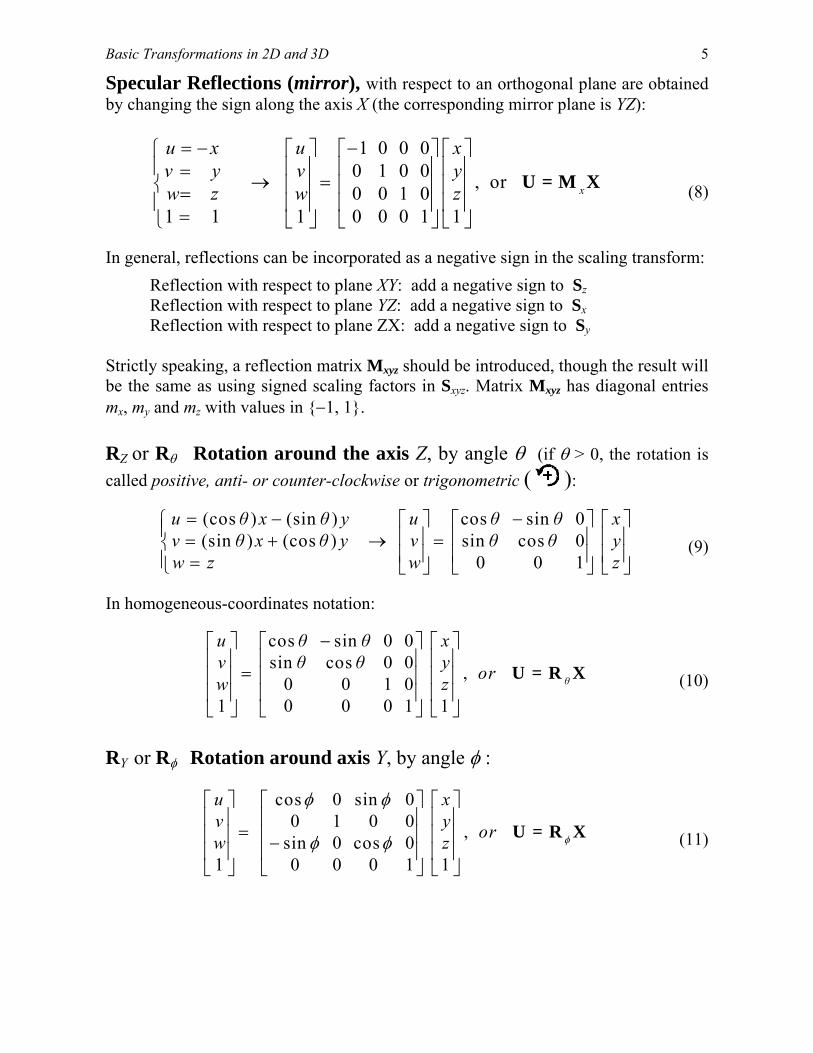
Specular Reflections (mirror), with respect to an orthogonal plane are obtained by changing the sign along the axis X (the corresponding mirror plane is YZ):
1 0 0 00 1 0 0 , or0 0 1 0
1 1 1 0 0 0 1 1x
u x u xv y v yw z w z
= − −⎧ ⎡ ⎤ ⎡ ⎤ ⎡ ⎤⎪ ⎢ ⎥ ⎢ ⎥ ⎢ ⎥= → =⎨ ⎢ ⎥ ⎢ ⎥ ⎢ ⎥=⎪ ⎢ ⎥ ⎢ ⎥ ⎢ ⎥
=⎩ ⎣ ⎦ ⎣ ⎦ ⎣ ⎦
U = M X (8)
In general, reflections can be incorporated as a negative sign in the scaling transform:
Reflection with respect to plane XY: add a negative sign to Sz Reflection with respect to plane YZ: add a negative sign to Sx Reflection with respect to plane ZX: add a negative sign to Sy
Strictly speaking, a reflection matrix Mxyz should be introduced, though the result will be the same as using signed scaling factors in Sxyz. Matrix Mxyz has diagonal entries mx, my and mz with values in {−1, 1}.
RZ or Rθ Rotation around the axis Z, by angle θ (if θ > 0, the rotation is called positive, anti- or counter-clockwise or trigonometric ( ):
(cos ) (sin ) cos sin 0(sin ) (cos ) sin cos 0
0 0 1
u θ x θ y u θ θ xv θ x θ y v θ θ yw z w z
= − −⎧ ⎡ ⎤ ⎡ ⎤ ⎡ ⎤⎪ ⎢ ⎥ ⎢ ⎥ ⎢ ⎥= + → =⎨⎢ ⎥ ⎢ ⎥ ⎢ ⎥⎪ =⎩ ⎣ ⎦ ⎣ ⎦ ⎣ ⎦
(9)
In homogeneous-coordinates notation:
cos sin 0 0sin cos 0 0 ,0 0 1 0
1 0 0 0 1 1θ
u θ θ xv θ θ y orw z
−⎡ ⎤ ⎡ ⎤ ⎡ ⎤⎢ ⎥ ⎢ ⎥ ⎢ ⎥
=⎢ ⎥ ⎢ ⎥ ⎢ ⎥⎢ ⎥ ⎢ ⎥ ⎢ ⎥⎣ ⎦ ⎣ ⎦ ⎣ ⎦
U = R X (10)
RY or Rφ Rotation around axis Y, by angle φ :
cos 0 sin 00 1 0 0 ,sin 0 cos 0
1 0 0 0 1 1
u xv y orw z φ
φ φ
φ φ
⎡ ⎤ ⎡ ⎤ ⎡ ⎤⎢ ⎥ ⎢ ⎥ ⎢ ⎥
=⎢ ⎥ ⎢ ⎥ ⎢ ⎥−⎢ ⎥ ⎢ ⎥ ⎢ ⎥⎣ ⎦ ⎣ ⎦ ⎣ ⎦
U = R X (11)
Basic Transformations in 2D and 3D 6
Computer Graphics - Tutorial by Jorge Marquez - CCADET UNAM 2011
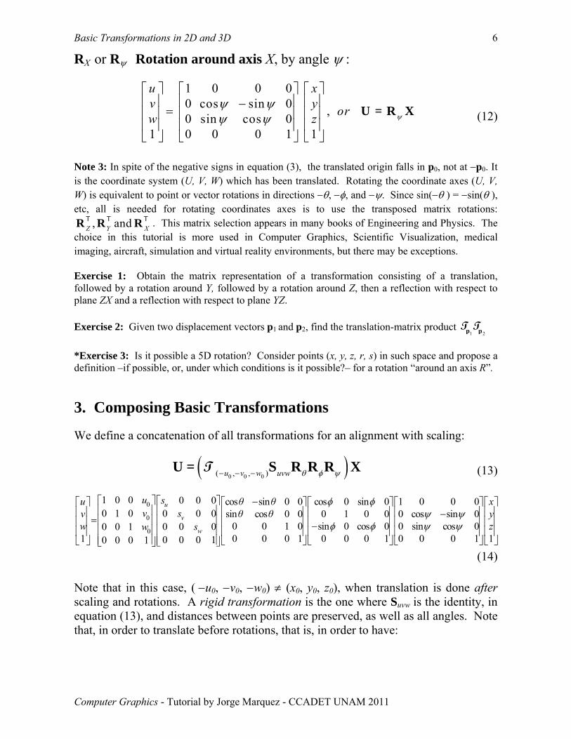
RX or Rψ Rotation around axis X, by angle ψ :
1 0 0 00 cos sin 0 ,0 sin cos 0
1 0 0 0 1 1
u xv y orw z ψ
ψ ψψ ψ
⎡ ⎤ ⎡ ⎤ ⎡ ⎤⎢ ⎥ ⎢ ⎥ ⎢ ⎥−=⎢ ⎥ ⎢ ⎥ ⎢ ⎥⎢ ⎥ ⎢ ⎥ ⎢ ⎥⎣ ⎦ ⎣ ⎦ ⎣ ⎦
U = R X (12)
Note 3: In spite of the negative signs in equation (3), the translated origin falls in p0, not at −p0. It is the coordinate system (U, V, W) which has been translated. Rotating the coordinate axes (U, V, W) is equivalent to point or vector rotations in directions −θ, −φ, and −ψ. Since sin(−θ ) = −sin(θ ), etc, all is needed for rotating coordinates axes is to use the transposed matrix rotations:
, andZ Y XR R RT T T . This matrix selection appears in many books of Engineering and Physics. The choice in this tutorial is more used in Computer Graphics, Scientific Visualization, medical imaging, aircraft, simulation and virtual reality environments, but there may be exceptions. Exercise 1: Obtain the matrix representation of a transformation consisting of a translation, followed by a rotation around Y, followed by a rotation around Z, then a reflection with respect to plane ZX and a reflection with respect to plane YZ. Exercise 2: Given two displacement vectors p1 and p2, find the translation-matrix product
1 2p pT T *Exercise 3: Is it possible a 5D rotation? Consider points (x, y, z, r, s) in such space and propose a definition –if possible, or, under which conditions is it possible?– for a rotation “around an axis R”. 3. Composing Basic Transformations We define a concatenation of all transformations for an alignment with scaling:
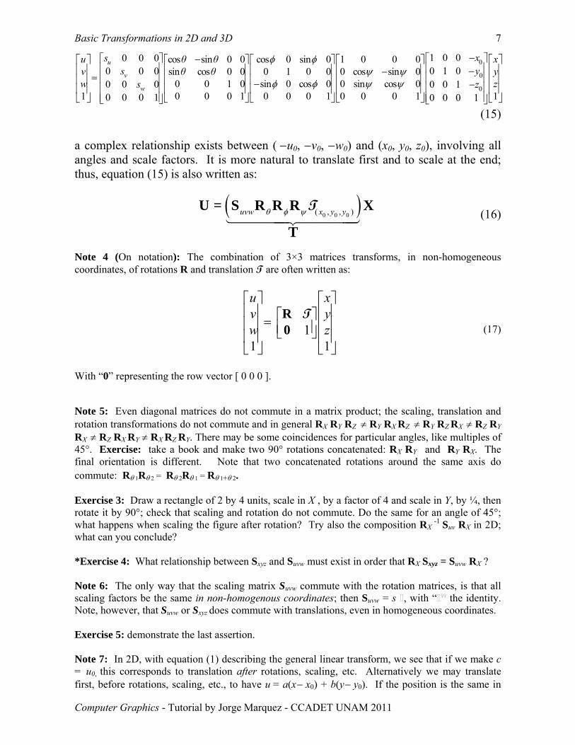
( )0 0 0( , , )u v w uvw θ φ ψ− − −U = S R R R XT (13)
0
0
0
1 0 0 0 0 0 cos sin 0 0 cos 0 sin 0 1 0 0 00 1 0 0 0 0 sin cos 0 0 0 1 0 0 0 cos sin 0
0 0 1 0 sin 0 cos 0 0 sin cos 00 0 00 0 11 0 0 0 1 0 0 0 1 0 0 0 1 10 0 0 10 0 0 1
u
v
w
u su θ θ xv sv θ θ y
w zsw
φ φψ ψ
φ φ ψ ψ
⎡ ⎤⎡ ⎤ −⎡ ⎤ ⎡ ⎤ ⎡ ⎤ ⎡ ⎤ ⎡⎢ ⎥ ⎢ ⎥⎢ ⎥ ⎢ ⎥ ⎢ ⎥ ⎢ ⎥−=⎢ ⎥ ⎢ ⎥⎢ ⎥ ⎢ ⎥ ⎢ ⎥ ⎢ ⎥−⎢ ⎥ ⎢ ⎥⎢ ⎥ ⎢ ⎥ ⎢ ⎥ ⎢ ⎥⎢ ⎥ ⎢ ⎥⎣ ⎦ ⎣ ⎦ ⎣ ⎦ ⎣ ⎦ ⎣⎣ ⎦⎣ ⎦
⎤⎢ ⎥⎢ ⎥⎢ ⎥
⎦
(14) Note that in this case, ( −u0, −v0, −w0) ≠ (x0, y0, z0), when translation is done after scaling and rotations. A rigid transformation is the one where Suvw is the identity, in equation (13), and distances between points are preserved, as well as all angles. Note that, in order to translate before rotations, that is, in order to have:
Basic Transformations in 2D and 3D 7
Computer Graphics - Tutorial by Jorge Marquez - CCADET UNAM 2011
0
0
0
1 0 00 0 0 cos sin 0 0 cos 0 sin 0 1 0 0 00 1 00 0 0 sin cos 0 0 0 1 0 0 0 cos sin 0
0 0 1 0 sin 0 cos 0 0 sin cos 00 0 0 0 0 11 0 0 0 1 0 0 0 1 0 0 0 10 0 0 1 0 0 0 1
u
v
w
xsu θ θ xysv θ θ y
w zs z
φ φψ ψ
φ φ ψ ψ
−⎡ ⎤⎡ ⎤ −⎡ ⎤ ⎡ ⎤ ⎡ ⎤ ⎡ ⎤⎢ ⎥⎢ ⎥⎢ ⎥ ⎢ ⎥ ⎢ ⎥ ⎢ ⎥ −−= ⎢ ⎥⎢ ⎥⎢ ⎥ ⎢ ⎥ ⎢ ⎥ ⎢ ⎥− −⎢ ⎥⎢ ⎥⎢ ⎥ ⎢ ⎥ ⎢ ⎥ ⎢ ⎥⎢ ⎥⎢ ⎥⎣ ⎦ ⎣ ⎦ ⎣ ⎦ ⎣ ⎦⎣ ⎦ ⎣ ⎦ 1
⎡ ⎤⎢ ⎥⎢ ⎥⎢ ⎥⎣ ⎦
(15) a complex relationship exists between ( −u0, −v0, −w0) and (x0, y0, z0), involving all angles and scale factors. It is more natural to translate first and to scale at the end; thus, equation (15) is also written as:
( )0 0 0( , , )uvw x y yθ φ ψU = S R R R X
T
T (16)
Note 4 (On notation): The combination of 3×3 matrices transforms, in non-homogeneous coordinates, of rotations R and translation T are often written as:
11 1
u xv yw z
⎡ ⎤ ⎡ ⎤⎢ ⎥ ⎢ ⎥⎡ ⎤=⎢ ⎥ ⎢ ⎥⎢ ⎥⎣ ⎦⎢ ⎥ ⎢ ⎥⎣ ⎦ ⎣ ⎦
R0
T (17)
With “0” representing the row vector [ 0 0 0 ].
Note 5: Even diagonal matrices do not commute in a matrix product; the scaling, translation and rotation transformations do not commute and in general RX RY RZ ≠ RY RX RZ ≠ RY RZ RX ≠ RZ RY
RX ≠ RZ RX RY ≠ RX RZ RY. There may be some coincidences for particular angles, like multiples of 45°. Exercise: take a book and make two 90° rotations concatenated: RX RY and RY RX. The final orientation is different. Note that two concatenated rotations around the same axis do commute: Rθ 1Rθ 2 = Rθ 2Rθ 1 = Rθ 1+θ 2. Exercise 3: Draw a rectangle of 2 by 4 units, scale in X , by a factor of 4 and scale in Y, by ¼, then rotate it by 90°; check that scaling and rotation do not commute. Do the same for an angle of 45°; what happens when scaling the figure after rotation? Try also the composition RX
-1 Suv RX in 2D; what can you conclude? *Exercise 4: What relationship between Sxyz and Suvw must exist in order that RX Sxyz = Suvw RX ? Note 6: The only way that the scaling matrix Suvw commute with the rotation matrices, is that all scaling factors be the same in non-homogenous coordinates; then Suvw = s , with “ the identity. Note, however, that Suvw or Sxyz does commute with translations, even in homogeneous coordinates. Exercise 5: demonstrate the last assertion.
Note 7: In 2D, with equation (1) describing the general linear transform, we see that if we make c = u0, this corresponds to translation after rotations, scaling, etc. Alternatively we may translate first, before rotations, scaling, etc., to have u = a(x− x0) + b(y− y0). If the position is the same in
Basic Transformations in 2D and 3D 8
Computer Graphics - Tutorial by Jorge Marquez - CCADET UNAM 2011
both translations (same u, v) after (coordinate system UVW) and before (coordinate system XYZ), we may eliminate u from both equations; if the scaling matrix is the identity, we must have ax + by + uo = a(x− x0) + b(y− y0), that is, uo = −ax − by0, similarly: vo = −dx − ey0. For scaling, however, no relationship is possible between a pre-rotation-plus-translation scaling Sxyz and a post-rotation-plus-translation scaling Suvw: the result is a particular case of a shear deformation.
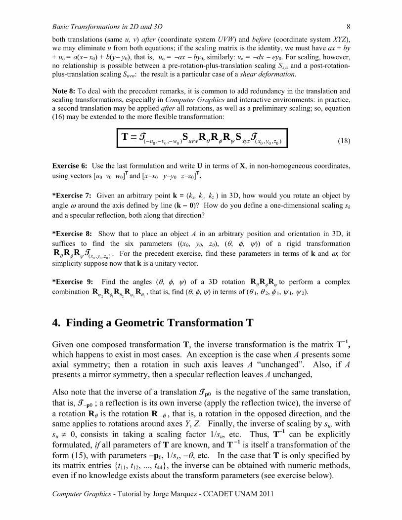
Note 8: To deal with the precedent remarks, it is common to add redundancy in the translation and scaling transformations, especially in Computer Graphics and interactive environments: in practice, a second translation may be applied after all rotations, as well as a preliminary scaling; so, equation (16) may be extended to the more flexible transformation:
0 0 0 0 0 0( , , ) ( , , )u v w uvw xyz x y zθ φ ψ− − −T S R R R S= T T (18)
Exercise 6: Use the last formulation and write U in terms of X, in non-homogeneous coordinates, using vectors [u0 v0 w0]T and [x−x0 y−y0 z−z0]T. *Exercise 7: Given an arbitrary point k = (kx, ky, kz ) in 3D, how would you rotate an object by angle ω around the axis defined by line (k − 0)? How do you define a one-dimensional scaling sk and a specular reflection, both along that direction? *Exercise 8: Show that to place an object A in an arbitrary position and orientation in 3D, it suffices to find the six parameters ((x0, y0, z0), (θ, φ, ψ)) of a rigid transformation
0 0 0( , , )x y zθ φ ψR R R T . For the precedent exercise, find these parameters in terms of k and ω; for simplicity suppose now that k is a unitary vector. *Exercise 9: Find the angles (θ, φ, ψ) of a 3D rotation θ φ ψR R R to perform a complex combination
2 1 2 1 1ψ φ θ ψ θR R R R R , that is, find (θ, φ, ψ) in terms of (θ 1, θ 2, φ 1, ψ 1, ψ 2).
4. Finding a Geometric Transformation T Given one composed transformation T, the inverse transformation is the matrix T−1, which happens to exist in most cases. An exception is the case when A presents some axial symmetry; then a rotation in such axis leaves A “unchanged”. Also, if A presents a mirror symmetry, then a specular reflection leaves A unchanged,
Also note that the inverse of a translation Tp0 is the negative of the same translation, that is, T−p0 ; a reflection is its own inverse (apply the reflection twice), the inverse of a rotation Rθ is the rotation R −θ , that is, a rotation in the opposed direction, and the same applies to rotations around axes Y, Z. Finally, the inverse of scaling by su, with su ≠ 0, consists in taking a scaling factor 1/su, etc. Thus, T−1 can be explicitly formulated, if all parameters of T are known, and T −1 is itself a transformation of the form (15), with parameters −p0, 1/sx, −θ, etc. In the case that T is only specified by its matrix entries {t11, t12, ..., t44}, the inverse can be obtained with numeric methods, even if no knowledge exists about the transform parameters (see exercise below).
Basic Transformations in 2D and 3D 9
Computer Graphics - Tutorial by Jorge Marquez - CCADET UNAM 2011
Exercise 10: applying the above remarks, and the fact that cos(−θ ) = cos(θ ), sin(−θ ) = −sin(θ ) (and similarly for angles φ, ψ), write T −1 in expanded form, as in equation (15), but remember to reverse the order of rotations from θ φ ψR R R to ψ φ θ− − −R R R , according to the matrix property (M1M2) −1 = M2
−1 M1−1 .
Given two objects A and B (where A could be B, after performing a given transformation on its set of points), we may want to find the transformation T (or T−1), where A and B are aligned. The problem may be formulated in general (even for non-linear transformations), as an optimization problem, in which, for example, some error metric between A and T(B) gives a criterion such that:
( ){ }min arg min , ( )metricError A B=T
T T (19)
Instead of “error” we may be interested in measuring similarity and the above expression reads as “the transformation which maximizes the similarity criterion between A and T(B)”:
( ){ }max arg max , ( )metricSimilarity A B=T
T T (20)
Many error and similarity criteria exist, especially when B and A are intrinsically different, and/or there is noise or error in their point representation. The above general formulation of equations (19) as well as its “max” counterpart (20) can be applied to non-linear transformations, that is geometric deformations or distortions, also known as warps, being unwarping their inversion. Note 9: Once we chose and fix the composition or nature of a given transformation T, it will be defined by its parameters, so equations (19) and (20) are often written in terms of finding the vector of parameters θ that minimizes the error-metric criterion. In our case, we may write θ = ( x0, y0, z0, ψ, φ, θ, su, sv, sw ), then T−1
has parameters ( −x0, −y0, −z0, −θ, −φ, −ψ, 1/su, 1/sv, 1/sw ), with rotations done in reverse order, as already mentioned. Exercise 11: Show that, in 2D, T=Rθ Sxy is always invertible, in non-homogeneous coordinates. Same question, using homogeneous coordinates for the matrix defined by T=RX Tp0. Let us first review direct, simple techniques for finding T, given A and B, or even when only a set of matching landmarks from A and B is known. Consider the case that the transformation T is unknown, but there are corresponding landmarks between A and B, and T is of the form shown in equation (16). Since nine parameters characterize an alignment with scaling, only three pairs of 3D landmarks (fiduciary points, “hitos” (in Spanish), or “bornes” (in French)) are needed to univocally determine the full transformation T, from a linear system of nine equations like (15), one for each pair {(xn, yn, zn, 1), (un, vn, wn, 1)}. However, this strictly requires that all landmarks match perfectly, even if A and B are very different.
Basic Transformations in 2D and 3D 10
Computer Graphics - Tutorial by Jorge Marquez - CCADET UNAM 2011
This is not always possible: some tolerance has to be introduced and any method to find T from three landmark matching is known as three-point registration. A way to obtain the translation parameters (x0, y0, z0), between two objects A and B, especially if their shapes are similar, is by making their geometric centroid (or center of mass, if mass distribution is uniform) be the same; one usually places the centroid of the source object as the origin; then (x0, y0, z0) is defined as the centroid of the target. The centroid of a set of points {( xn, yn, zn)} n=1,..., N is defined as
( ) ( ) ( )1
, , 1 / , , N
C C C C n n nn
x y z N x y z=
= = ∑p (21)
The centroid may be approximated from the landmarks only, if they are representative of the objects. A translation may be also defined by simply taking the difference of position from one pair of corresponding landmarks, if they are robust. A generic solution to the problem of finding the composed rotation ( θ φ ψR R R ), consists in obtaining the principal axes of each object, and make their orientations be the same (herein the term alignment). The Principal Component Analysis (PCA) is the most common method to find such directions for a coarse alignment. The eigenvectors determine the orientation, and the eigenvalues relate with the scaling factors. An advantage is that, if landmarks are not robust, many more sample points can be used for the PCA method and there is no need for pairing such points. If an axial symmetry exists in the object, two axes can be the same, and the rotation will not be completely determined. As with translation, an orientation may also be defined by simply taking the 3D rotation needed to perfectly match three corresponding landmarks, if they are robust (reliable), and no large scaling is involved. Specular reflections, with respect to planes UV, VW and WU, corresponding to a change of sign in the coordinates w, v and u, respectively, may be difficult to determine automatically, without a priori information. Information on landmark correspondence is required, and it is also often the case that there is only reflection in one axis. This is a consequence that combinations of two reflections are equivalent to some additional rotation of π radians. PCA is treated in another tutorial. Once the composed rotation is found, and reflections are taken into account, the positive scaling factors are easily calculated from comparing the bounding boxes of each object in the UVW system of coordinates; these boxes are defined as:
min max min max min max
min max min max min max
( ) [ , ] [ , ] [ , ]
( ) [ , ] [ , ] [ , ]
A A A A A A
B B B B B B
Bbox A u u v v w w
Bbox B u u v v w w
= × ×
= × × (22)
Where “×” denotes the Cartesian product and:
Basic Transformations in 2D and 3D 11
Computer Graphics - Tutorial by Jorge Marquez - CCADET UNAM 2011
{ } { }min maxmin | , max |A Au uu A u A= ∈ = ∈p p p p , etc. (23)
Then, the scaling factors su, sv, sw in equation (14) are calculated from:
max min max min max min
max min max min max min
, and B B B B B Bu v w
A A A A A A
u u v v w ws s su u v v w w
− − −= = =
− − − (24)
If the target B is half the size of the source A, all scale factors are equal to ½. Note 10: Noise and/or error variations in points in A and B, as well as rounding errors during transformation operations, make the above method not very robust, especially if A is very small, compared to B and to noise or error in the coordinate values. Equations (22) to (24) also rely on just a few points, in the best case. The second, third and further minima and maxima would help to improve equation (23), or even better, by obtaining a trimmed average of the N extrema, with N such that the uncertainty on (22) and (23) falls below some given tolerance. The above calculations for finding a proper translation, and alignment by PCA and for finding scaling factors, can be alternatively performed by applying Least Squared Errors methods, which is a special case of the general optimization formulas (19) and (20), and by sampling the sets A, B, if no particular pairs of landmarks are extracted. Sampling introduces statistical analysis as the natural way to deal with random variation, and reduces complexity. Linear regression is a typical example; in this case, several points allow to better estimate the line-equation parameters, even if only two are strictly needed, when there is zero noise. Exercise 12: An implicit representation of transformation T, formulated as in equation (16), is the set of sixteen matrix entries {t11, t12,..., t44}. Does the homogeneous-coordinate representation restricts, in some way, the values of the last row of entries t41, t42, t43, t44, or any other entries? We also know that the same T is completely determined by the nine parameters θ = ( x0, y0, z0, ψ, φ, θ, su, sv, sw ), which constitutes an explicit representation. Given the matrix entries, find θ in terms of {t11, t12, ..., t44} if possible, or determine what other information is required. See also Appendix B. Note 11: When A and B are very different, or/and there is noise or some shape distortion, and thus, no exact feature matching can be obtained, several techniques exist. A common one is similar to linear regression analysis where a line is fitted to a set of points with largely more than two points. This is a statistical framework and the alignment is performed by minimizing a Mean Squared Error (Least MSE) criterion, where several points from A and B are taken even if “only three” would be needed if they match perfectly, without noise or error.
Basic Transformations in 2D and 3D 12
Computer Graphics - Tutorial by Jorge Marquez - CCADET UNAM 2011
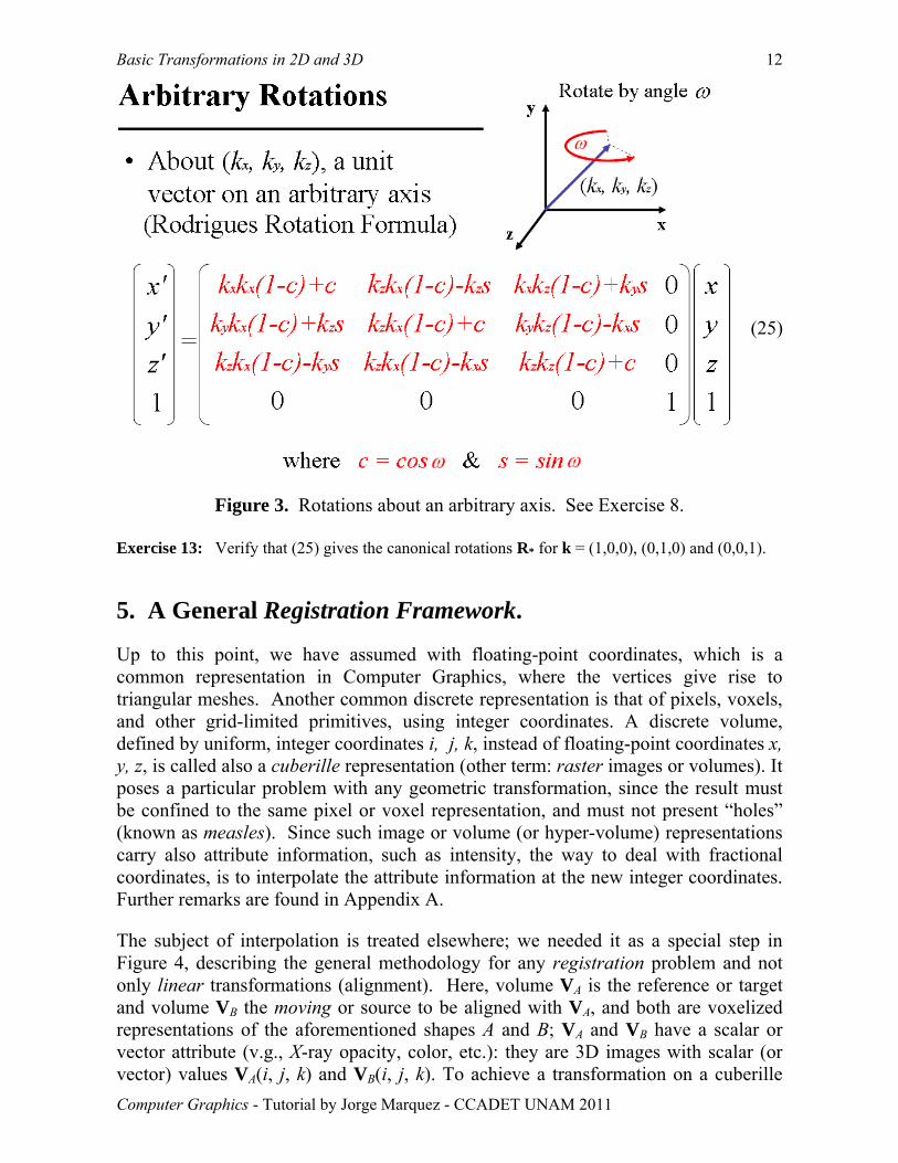
(25)
Figure 3. Rotations about an arbitrary axis. See Exercise 8. Exercise 13: Verify that (25) gives the canonical rotations R* for k = (1,0,0), (0,1,0) and (0,0,1). 5. A General Registration Framework. Up to this point, we have assumed with floating-point coordinates, which is a common representation in Computer Graphics, where the vertices give rise to triangular meshes. Another common discrete representation is that of pixels, voxels, and other grid-limited primitives, using integer coordinates. A discrete volume, defined by uniform, integer coordinates i, j, k, instead of floating-point coordinates x, y, z, is called also a cuberille representation (other term: raster images or volumes). It poses a particular problem with any geometric transformation, since the result must be confined to the same pixel or voxel representation, and must not present “holes” (known as measles). Since such image or volume (or hyper-volume) representations carry also attribute information, such as intensity, the way to deal with fractional coordinates, is to interpolate the attribute information at the new integer coordinates. Further remarks are found in Appendix A. The subject of interpolation is treated elsewhere; we needed it as a special step in Figure 4, describing the general methodology for any registration problem and not only linear transformations (alignment). Here, volume VA is the reference or target and volume VB the moving or source to be aligned with VA, and both are voxelized representations of the aforementioned shapes A and B; VA and VB have a scalar or vector attribute (v.g., X-ray opacity, color, etc.): they are 3D images with scalar (or vector) values VA(i, j, k) and VB(i, j, k). To achieve a transformation on a cuberille
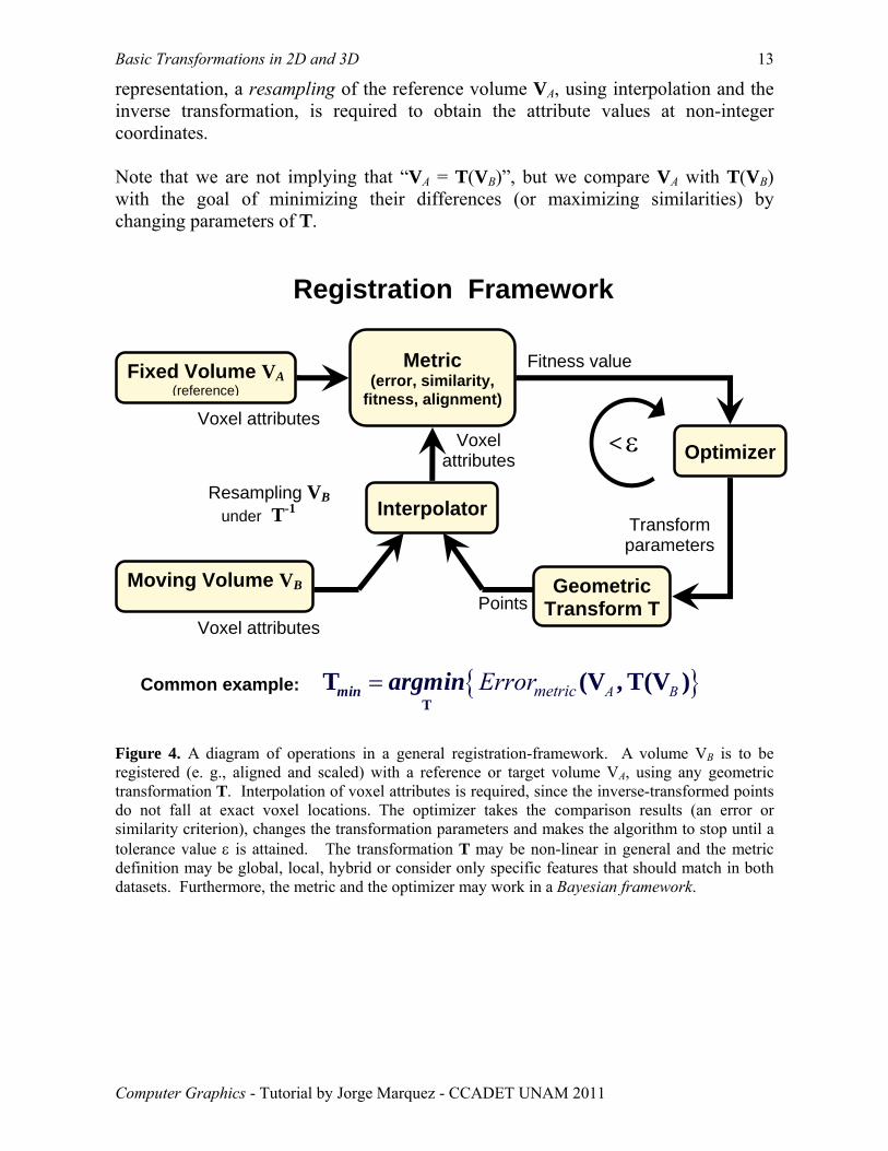
Basic Transformations in 2D and 3D 13
Computer Graphics - Tutorial by Jorge Marquez - CCADET UNAM 2011
representation, a resampling of the reference volume VA, using interpolation and the inverse transformation, is required to obtain the attribute values at non-integer coordinates. Note that we are not implying that “VA = T(VB)”, but we compare VA with T(VB) with the goal of minimizing their differences (or maximizing similarities) by changing parameters of T.
Figure 4. A diagram of operations in a general registration-framework. A volume VB is to be registered (e. g., aligned and scaled) with a reference or target volume VA, using any geometric transformation T. Interpolation of voxel attributes is required, since the inverse-transformed points do not fall at exact voxel locations. The optimizer takes the comparison results (an error or similarity criterion), changes the transformation parameters and makes the algorithm to stop until a tolerance value ε is attained. The transformation T may be non-linear in general and the metric definition may be global, local, hybrid or consider only specific features that should match in both datasets. Furthermore, the metric and the optimizer may work in a Bayesian framework.
Fixed Volume VA (reference)
Metric (error, similarity,
fitness, alignment)
Optimizer
Interpolator
Geometric Transform T
Moving Volume VB
Fitness value
Voxel attributes
Voxel attributes Points
Transform parameters
Voxel attributes
Registration Framework
{ }A BmetricError=T
T (V , T(V )min argminCommon example:
Resampling VB under T-1
< ε
Basic Transformations in 2D and 3D 14
Computer Graphics - Tutorial by Jorge Marquez - CCADET UNAM 2011
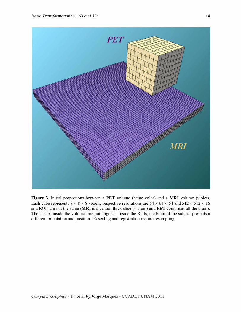
Figure 5. Initial proportions between a PET volume (beige color) and a MRI volume (violet). Each cube represents 8 × 8 × 8 voxels; respective resolutions are 64 × 64 × 64 and 512 × 512 × 16 and ROIs are not the same (MRI is a central thick slice (4-5 cm) and PET comprises all the brain). The shapes inside the volumes are not aligned. Inside the ROIs, the brain of the subject presents a different orientation and position. Rescaling and registration require resampling.
Basic Transformations in 2D and 3D 15
Computer Graphics - Tutorial by Jorge Marquez - CCADET UNAM 2011
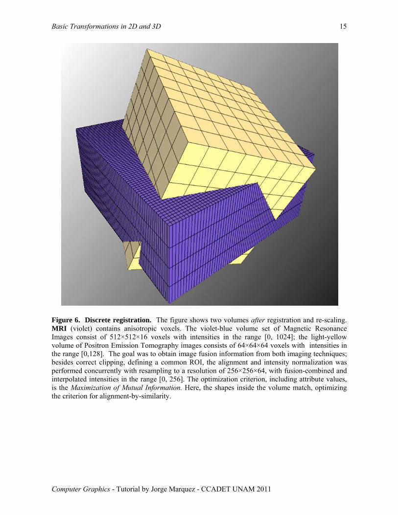
Figure 6. Discrete registration. The figure shows two volumes after registration and re-scaling. MRI (violet) contains anisotropic voxels. The violet-blue volume set of Magnetic Resonance Images consist of 512×512×16 voxels with intensities in the range [0, 1024]; the light-yellow volume of Positron Emission Tomography images consists of 64×64×64 voxels with intensities in the range [0,128]. The goal was to obtain image fusion information from both imaging techniques; besides correct clipping, defining a common ROI, the alignment and intensity normalization was performed concurrently with resampling to a resolution of 256×256×64, with fusion-combined and interpolated intensities in the range [0, 256]. The optimization criterion, including attribute values, is the Maximization of Mutual Information. Here, the shapes inside the volume match, optimizing the criterion for alignment-by-similarity.
Basic Transformations in 2D and 3D 16
Computer Graphics - Tutorial by Jorge Marquez - CCADET UNAM 2011
APPENDIX – Additional Remarks and Exercises. A. Discrete Scaling and Resampling: Upsampling and Downsampling.
A geometric transformation T is applied directly to finite sets of coordinate points P = {pn}n = 0,…, N-1, with pn ∈ 3. These may be vertices of lines, triangles or other polygons, which in turn may constitute other objects. Such primitives provide a structure to P. Note that there is no intrinsic grid representation of such objects (usually, manifolds). Thus, besides clouds of points, any continuous object (manifold) represented by a structured set P is directly transformed by T. Such manifolds include: vectorized contours (polylines), any shape defined by generalized polygons, 3D polytopes and surface meshes made of triangles or simple polygons.
Raster (pixelized or voxelized) curves, images, surfaces and volumes are samples from a continuous representation, arranged on a discrete grid in 3. They usually bear also a scalar or vector attribute per pixel (voxel), such as density or color and constitute scalar o vector fields. Applying T directly on such point samples and discrete fields creates holes on the resulting grid, among other discretization- related problems. The first is known as the measles problem. Manifolds may also bear an attribute per vertex, but if such value changes along the manifold primitive (e. g., triangles) then manifolds have to be treated in a similar fashion to discrete fields.
Scaling, rotating or other geometric transformations require rebuilding the discrete raster information (images or maps, volumes or fields, etc.), by interpolating attribute values for the new pixel (voxel) grid, from the source grid, using T −1, which may generates non integer points for which attribute values have to be interpolated from neighboring integer coordinates. Such operations (transform plus interpolations) are called resampling.
In particular, to just increase or to decrease n-fold the resolution of a discrete image (or volume), with n an integer, the interpolation of order zero consists in replicating pixels (voxels) n times for an increase in resolution. Decreasing n-fold requires skipping n pixels (an integer way to “divide by n”). Such discrete scaling, when multiplying resolution by a factor n (magnification) is called upsampling and is often represented as “I↑n” for an image I. If the resolution is divided by a factor n (decimation or reduction), it is called downsampling (or subsampling) and is often represented as “I↓n”. If n is not integer, the terminology still applies, but an interpolation of higher order improves approximation and reduces discretization artifacts.
Note 12: In signal analysis, upsampling and downsampling are defined as “the process of increasing (decreasing, respectively) the sampling rate of a signal”. In spatial domain such sampling rate determines the size of pixels or voxels for a different resolution. A fractional
Basic Transformations in 2D and 3D 17
Computer Graphics - Tutorial by Jorge Marquez - CCADET UNAM 2011
scaling n/m is easily achieved by upsampling data by an integer factor n, then downsampling by an integer factor m.
The discrete representation of an image or volume (“pixelization” or “voxelization”) will be more noticeable under zero-order interpolations, since pixel or voxel replication increases the size of the staircase artifacts. Higher order interpolations and antialiasing techniques smooth out such artifacts in computer graphics renderings, but the smoothing (blur) will then be more evident. There are upsampling techniques (magnification or zoom-in) that preserve discontinuities and reduce aliasing. Some techniques use vectorized representations; other use anisotropic filtering to preserve sharp corners and borders. A very effective but scarcely known technique is the morphological zoom; it applies upsampling by any factor in the Euclidean distance transform (EDT) and resampling with bilinear or bicubic (trilinear or tricubic in 3D) interpolation in the EDT domain.
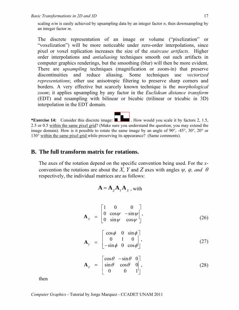
*Exercise 14: Consider this discrete image: . How would you scale it by factors 2, 1.5, 2.5 or 0.5 within the same pixel grid? (Make sure you understand the question; you may extend the image domain). How is it possible to rotate the same image by an angle of 90°, -45°, 30°, 20° or 130° within the same pixel grid while preserving its appearance? (Same comments). B. The full transform matrix for rotations.
The axes of the rotation depend on the specific convention being used. For the x-convention the rotations are about the X, Y and Z axes with angles ψ, φ, and θ respectively, the individual matrices are as follows:
XZ Y=A A A A , with
1 0 00 cos sin ,0 sin cos
cos 0 sin0 1 0 ,
sin 0 cos
cos sin 0sin cos 0 ,
0 0 1
X
Y
Z
ψ ψψ ψ
φ φ
φ φ
θ θθ θ
⎡ ⎤⎢ ⎥−= ⎢ ⎥⎣ ⎦
⎡ ⎤⎢ ⎥
= ⎢ ⎥−⎣ ⎦
−⎡ ⎤⎢ ⎥=⎢ ⎥⎣ ⎦
A
A
A
(26)
(27)
(28)
then
Basic Transformations in 2D and 3D 18
Computer Graphics - Tutorial by Jorge Marquez - CCADET UNAM 2011
cos cos cos sin sin sin cos cos sin cos sin sinsin cos sin sin sin cos cos sin sin cos cos sin
sin cos sin cos cos
θ φ θ φ ψ θ ψ θ φ ψ θ ψθ φ θ φ ψ θ ψ θ φ ψ θ ψ
φ φ ψ φ ψ
− ++ −
−
⎡ ⎤⎢ ⎥=⎢ ⎥⎣ ⎦
A (29)
Note 13: If coordinate rotation is intended (active versus passive rotations), the transposed matrices should be used.
Note 14: For left-handed sign convention(s), change the sign in all sin(.) entries.
**Exercise 15: Verify equation (29). HINT: simplify notation using for example “sψ” for sin(ψ), etc. Compare with the definitions given in the Wikipedia for the article http://en.wikipedia.org/wiki/Rotation_formalisms_in_three_dimensions Besides scrambling the angle notation of this tutorial, the authors assume a clockwise orientation for all or some angles to rotate the coordinate axes (see note 3). Is that all? They also talk about assuming a “right-hand convention”? Is there any inconsistency here or within the article of the Wikipedia? How can you correct it or interpret such inconsistencies -if any?
Exercise 16: Complete the angle orientation indications (arc-with-arrow) around axes Y and Z in figure 1, as done with axis X. Verify against canonical rotations by applying them about axes Y and Z to points (0, 1, 0), (0, 0, 1) and (0, 1, 1). Do the same for rotations defined in the article cited in Exercise 15.
*Exercise 17: Write A-1 in terms of θ, φ and ψ (see also Exercises 11 and 12).
*Exercise 18: Generalize the above to quaternion matrices T (i.e., homogeneous coordinates) to include in T a translation matrix, before all rotations and a scaling matrix after all rotations, as in equation (15) and write both, T and T -1 in terms of ((x0, y0, z0), (θ, φ, ψ), (su, sv, sw)). *Exercise 19: Compare with the case of performing the at-the-end translation (u0, v0, w0) and scaling first with scale factors (sx, sy, sz); almost as in equation (14). Note that it is equivalent to renaming T as T -1 and vice versa (watch out for signs, inversions and proper notation in XYZ and UVW spaces). This particular order is often used when dealing with eigenvectors and eigenvalues of the ellipsoid of inertia and in Principal Component Analysis.
*Exercise 20: Write the A matrix in homogeneous coordinates. Find and discuss any relationships with equation (29), for three arbitrary orthogonal rotations. *Exercise 22: Write the A matrix for a left-handed system of coordinates (there are other cases). Relate angle orientations (trigonometric versus clockwise) with both conventions. Enumerate all possible angle conventions and write their corresponding AX, AY, and AZ matrices.
Exercise 22: We have used in this tutorial the right-hand rule with positive sign convention. Alternative systems of orthogonal rotations include rotation combinations such as AY AZ AX, etc., but also combining changes in one or more sign angles, such as AX
T AZ AYT. Euler
rotations introduce still other matrix combinations. Calculate the global transformations (equivalents to equation (29)) for all rotation combinations and all negative and positive sign combinations. Hint: Extensively apply the transposition property: (MaMb) T
= MbTMa
T. At
Basic Transformations in 2D and 3D 19
Computer Graphics - Tutorial by Jorge Marquez - CCADET UNAM 2011
least find to what rotation combination (and sign combinations) correspond the global matrix that is equal to AT, with A given by (29), note that AT is not “AZ
TAYTAX
T”.
Exercise 23: Investigate what is a “flip”, a “flop” and a “slant” and define them in terms of basic transformations introduced in this tutorial. Are there other synonyms or concepts involving known geometric transformations? What about “yaw”, “roll” and “pitch” also known as “heading”, “elevation” and “bank”? How do they relate with canonical rotations on this tutorial. Exercise 24: Investigate what are intrinsic and extrinsic rotations and relate them with canonical rotations in this tutorial. *Exercise 25: Study the article http://en.wikipedia.org/wiki/Euler_angles as well as the article indicated in Exercise 15 and find transformation relationships among the Euler-angle rotations and the canonical rotations as defined in this tutorial. For still more information, within the Wikipedia, take a look to article http://en.wikipedia.org/wiki/Rotation_matrix. *Exercise 26: Research or deduce yourself a formulation for shear transformations in 2D and 3D, first using a standard system of equations, as in equation (2). Can the shear transformations be included as pre- or post-multiplying matrix terms in any of equations (13) to (16), (18) and (29)? Are the shear transformations linear? Discuss and write the pertinent equations, including shears, if the answer is either yes or no (that is, how to include, whenever possible, shears in a matrix formulation).