basics and application of ground- penetrating radar as a...

8

Basics and Application of Ground- Penetrating Radar as a Tool for

Monitoring Irrigation Process

Kazunori Takahashi1, Jan Igel1, Holger Preetz1 and Seiichiro Kuroda2 1Leibniz Institute for Applied Geophysics

2National Institute for Rural Engineering 1Germany

2Japan

1. Introduction

Ground-penetrating radar (GPR) is a geophysical method that employs an electromagnetic technique. The method transmits and receives radio waves to probe the subsurface. One of the earliest successful applications was measuring ice thickness on polar ice sheets in 1960s (Knödel et al., 2007). Since then, there have been rapid developments in hardware, measurement and analysis techniques, and the method has been extensively used in many applications, such as archaeology, civil engineering, forensics, geology and utilities detection (Daniels, 2004).

There are a variety of methods to measure soil water content. The traditional method is to dry samples from the field and compare the weights of the samples before and after drying. This method can analyse sampled soils in detail and the results may be accurate. A classical instrument for in situ measurements is the tensiometer, which measures soil water tension. These methods have the disadvantages of being destructive and time-intensive, and thus it is impossible to capture rapid temporal changes. Therefore, a number of sophisticated physical methods have been developed for non-destructive in situ measurements. One of these methods is time domain reflectometry (TDR), which has been widely used for determining soil moisture since the 1980s (Topp et al., 1980; Noborio, 2001; Robinson et al., 2003). TDR measurements are easy to carry out and cost effective, however they are not suitable for obtaining the high-resolution soil water distribution because either a large number of probes have to be installed or a single measurement has to be repeated at various locations. In addition, TDR measurements are invasive; the probes must be installed into soil, which may slightly alter the soil properties. GPR has the potential to overcome these problems and is considered one of the most suitable methods for monitoring soil water content during and after irrigation because of the following features:

• The GPR response reflects the dielectric properties of soil that are closely related to its water content.

• GPR data acquisition is fast compared to other geophysical methods. This feature enables measurements to be made quickly and repeatedly, yielding high temporal resolution monitoring. This is very important for capturing rapid changes.

www.intechopen.com

Problems, Perspectives and Challenges of Agricultural Water Management

156

• GPR can be used as a completely non-invasive method. The antennas do not have to touch the ground and thus it does not disturb the natural soil conditions.

• GPR systems are compact and easy to use compared to other geophysical methods. This feature enables scanning over a wide area and the collection of 2D or 3D data. Further, the distribution of soil properties can be obtained with high spatial resolution.

The objective of this chapter is to provide the basics of GPR and examples of its application. Readers who are interested in this measurement technique can find more detailed and useful information in the references listed at the end of the chapter.

2. Basic principles of GPR

A GPR system consists of a few components, as shown in Fig. 1, that emit an electromagnetic wave into the ground and receive the response. If there is a change in electric properties in the ground or if there is an anomaly that has different electric properties than the surrounding media, a part of the electromagnetic wave is reflected back to the receiver. The system scans the ground to collect the data at various locations. Then a GPR profile can be constructed by plotting the amplitude of the received signals as a function of time and position, representing a vertical slice of the subsurface, as shown in Fig. 2. The time axis can be converted to depth by assuming a velocity for the electromagnetic wave in the subsurface soil.

Fig. 1. Block diagram of a GPR system.

Fig. 2. A GPR profile obtained with a 1.5 GHz system scanned over six objects buried in sandy soil. The signal amplitude is plotted as a function of time (or depth) and position. Relatively small objects are recognised by hyperbolic-shaped reflections. Reflections from the ground surface appear as stripes at the top of the figure.

www.intechopen.com

Basics and Application of Ground-Penetrating Radar as a Tool for Monitoring Irrigation Process

157

2.1 Electromagnetic principles of GPR

2.1.1 Electromagnetic wave propagation in soil

The propagation velocity v of the electromagnetic wave in soil is characterised by the

dielectric permittivity ε and magnetic permeability µ of the medium:

0 0

1 1

r r

vεµ ε ε µ µ

= =

(1)

where ε0 = 8.854 x 10-12 F/m is the permittivity of free space, εr = ε/ε0 is the relative

permittivity (dielectric constant) of the medium, µ0 = 4π x 10-7 H/m is the free-space

magnetic permeability, and µr = µ/µ0 is the relative magnetic permeability. In most soils,

magnetic properties are negligible, yielding µ = µ0, and Eq. 1 becomes

r

cv

ε=

(2)

where c = 3 x 108 m/s is the speed of light. The wavelength λ is defined as the distance of the wave propagation in one period of oscillation and is obtained by

2v

f

πλ

ω εµ= =

(3)

where f is the frequency and ω = 2πf is the angular frequency.

In general, dielectric permittivity ε and electric conductivity σ are complex and can be expressed as

jε ε ε′ ′′= −

(4)

jσ σ σ′ ′′= −

(5)

where ε’ is the dielectric polarisation term, ε” represents the energy loss due to the

polarisation lag, σ’ refers to ohmic conduction, and σ” is related to faradaic diffusion (Knight & Endres, 2005). A complex effective permittivity expresses the total loss and storage effects of the material as a whole (Cassidy, 2009):

e jσ σ

ε ε εω ω

′′ ′ ′ ′′= + − + (6)

The ratio of the imaginary and real parts of the complex permittivity is defined as tan δ (loss tangent):

tan

ε σδ

ε ωε

′′ ′= ≅

′ ′ (7)

www.intechopen.com


158

When ε” and σ” are small, it is approximated as the right most expression. In the plane-wave solution of Maxwell’s equations, the electric field E of an electromagnetic wave that is travelling in z-direction is expressed as

( ) ( )

0,j t kz

E z t E eω −

= (8)

where E0 is the peak signal amplitude and k ω εµ= is the wavenumber, which is complex

if the medium is conductive, and it can be separated into real and imaginary parts:

k jα β= +

(9)

The real part α and imaginary part β are called the attenuation constant (Np/m) and phase constant (rad/m), respectively, and given as follows:

( )

1 221 tan 1

2

ε µα ω δ

′ = + − (10)

( )

1 221 tan 1

2

ε µβ ω δ

′ = + + (11)

The attenuation constant can be expressed in dB/m by α’ = 8.686α. The inverse of the attenuation constant:

1δ

α=

(12)

is called the skin depth. It gives the depth at which the amplitude of the electric field decay is 1/e (~ -8.7 dB, ~ 37%). It is a useful parameter to describe how lossy the medium is. Table 1 provides the typical range of permittivity, conductivity and attenuation of various materials.

Material Relative permittivity Conductivity [S/m]

Attenuation constant [dB/m]

Air 1 0 0 Freshwater 81 10-6-10-2 0.01 Clay, dry 2-6 10-3-10-1 10-50 Clay, wet 5-40 10-1-10-0 20-100 Sand, dry 2-6 10-7-10-3 0.01-1 Sand, wet 10-30 10-3-10-2 0.5-5

Table 1. Typical range of dielectric characteristics of various materials measured at 100 MHz (Daniels, 2004; Cassidy, 2009).

2.1.2 Reflection and transmission of waves

GPR methods usually measure reflected or scattered electromagnetic signals from changes in the electric properties of materials. The simplest scenario is a planar boundary between

www.intechopen.com


159

two media with different electric properties as shown in Fig. 3, which can be seen as a layered geologic structure.

Fig. 3. Reflection and transmission of a normally incident electromagnetic wave to a planar interface between two media.

When electromagnetic waves impinge upon a planar dielectric boundary, some energy is reflected at the boundary and the remainder is transmitted into the second medium. The relationships of the incident, reflected, and transmitted electric field strengths are given by

i r tE E E= + (13)

r iE R E= ⋅ (14)

t iE T E= ⋅ (15)

respectively, where R is the reflection coefficient and T is the transmission coefficient. In the case of normal incidence, illustrated in Fig. 3, the reflection and transmission coefficients are given as

2 1

2 1

Z ZR

Z Z

−=

+

(16)

2

2 1

21

ZT R

Z Z= − =

+ (17)

where Z1 and Z2 are the intrinsic impedances of the first and second media, respectively,

and Z µ ε= . In a low-loss non-conducting medium, the reflection coefficient may be

simplified as (Daniels, 2004)

1 2

1 2

r r

r r

Rε ε

ε ε

−≅

+ (18)

2.2 GPR systems

A GPR system is conceptually simple and consists of four main elements: the transmitting unit, the receiving unit, the control unit and the display unit (Davis & Annan, 1989), as

www.intechopen.com


160

depicted in Fig. 1. The basic type of GPR is a time-domain system in which a transmitter generates pulsed signals and a receiver samples the returned signal over time. Another common type is a frequency-domain system in which sinusoidal waves are transmitted and received while sweeping a given frequency. The time-domain response can be obtained by an inverse Fourier transform of the frequency-domain response.

GPR systems operate over a finite frequency range that is usually selected from 1 MHz to a few GHz, depending on measurement requirements. A higher frequency range gives a narrower pulse, yielding a higher time or depth resolution (i.e., range resolution), as well as lateral resolution. On the other hand, attenuation increases with frequency, therefore high-frequency signal cannot propagate as far and the depth of detection becomes shallower. If a lower frequency is used, GPR can sample deeper, but the resolution is lower.

Antennas are essential components of GPR systems that transmit and receive electromagnetic waves. Various types of antennas are used for GPR systems, but dipole and bowtie antennas are the most common. Most systems use two antennas: one for transmitting and the other for receiving, although they can be packaged together. Some commercial GPR systems employ shielded antennas to avoid reflections from objects in the air. The antenna gain is very important in efficiently emitting and receiving the electromagnetic energy. Antennas with a high gain help improve the signal-to-noise ratio. To achieve a higher antenna gain, the size of an antenna is determined by the operating frequency. A lower operating frequency requires larger antennas. Small antennas make the system compact, but they have a low gain at lower frequencies.

2.3 GPR surveys

GPR surveys can be categorised into reflection and transillumination measurements (Annan, 2009). Reflection measurements commonly employ configurations called common-offset and common midpoint. If antennas are placed on the ground, there are propagation paths both in and above the ground, as shown in Fig. 4. Transillumination measurements are usually carried out using antennas installed into trenches or drilled wells.

Fig. 4. Propagation paths of electromagnetic waves for a surface GPR survey with a layered structure in the subsurface.

2.3.1 Common-offset (CO) survey

In a common-offset survey, a transmitter and receiver are placed with a fixed spacing. The transmitter and receiver scan the survey area, keeping the spacing constant and acquiring the data at each measurement location, as depicted in Fig. 5. For a single survey line, the acquired GPR data corresponds to a 2D reflectivity map of the subsurface below the

www.intechopen.com


161

scanning line, i.e., a vertical slice (e.g., Fig. 2). By setting multiple parallel lines, 3D data can be obtained and horizontal slices and 3D maps can be constructed.

2.3.2 Common midpoint (CMP) survey

In a common midpoint survey, a separate transmitter and receiver are placed on the ground.

The separation between the antennas is varied, keeping the centre position of the antennas

constant. With varying separation and assuming a layered subsurface structure, various

signal paths with the same point of reflection are obtained and the data can be used to

estimate the radar signal velocity distribution versus subsurface depth (e.g., Annan, 2005;

Annan, 2009). The schematic configuration of a CMP survey is shown in Fig. 5. When the

transmitter is fixed, instead of being moved from the midpoint together with the receiver,

and if only the receiver is moved away from the transmitter, the setup is called a wide-angle

reflection and refraction (WARR) gather.

Fig. 5. Schematic illustrations of common-offset (left) and common midpoint (right) surveys. Tx and Rx indicate the transmitting and receiving antennas, respectively. Antennas are scanned with a fixed spacing S in the common-offset configuration, while the spacing is varied as shown with S1, S2, S3 … with respect to the middle position in the common midpoint configuration.

2.3.3 Transillumination measurements

Zero-offset profiling (ZOP) uses a configuration where the transmitter and receiver are

moved in two parallel boreholes with a constant distance (Fig. 6, left), resulting in parallel

raypaths in the case of homogeneous subsurface media. This setup is a simple and quick

way to locate anomalies.

Transillumination multioffset gather surveying provides the basis of tomographic imaging.

The survey measures transmission signals through the volume between boreholes with

varying angles (Fig. 6, right). Tomographic imaging constructed from the survey data can

provide the distribution of dielectric properties of the measured volume.

2.4 Physical properties of soil

As seen in the previous section, the electric and magnetic properties of a medium influence

the propagation and reflection of electromagnetic waves. These properties are dielectric

permittivity, electric conductivity and magnetic permeability.

www.intechopen.com


162

Fig. 6. Schematic illustrations of transillumination zero-offset profiling (left) and transillumination multioffset gather (right) configurations.

2.4.1 Dielectric permittivity

Permittivity describes the ability of a material to store and release electromagnetic energy in

the form of electric charge and is classically related to the storage ability of capacitors

(Cassidy, 2009). Permittivity greatly influences the electromagnetic wave propagation in

terms of velocity, intrinsic impedance and reflectivity. In natural soils, dielectric permittivity

might have a larger influence than electric conductivity and magnetic permeability (Lampe

& Holliger, 2003; Takahashi et al., 2011).

Soil can be regarded as a three-phase composite with the soil matrix and the pore space that

is filled with air and water. The pore water phase of soil can be divided into free water and

bound water that is restricted in mobility by absorption to the soil matrix surface. The

relative permittivity (dielectric constant) of air is 1, is between 2.7 and 10 for common

minerals in soils and rocks (Ulaby et al., 1986), while water has a relative permittivity of 81,

depending on the temperature and frequency. Thus, the permittivity of water-bearing soil is

strongly influenced by its water content (Robinson et al., 2003). Therefore, by analysing the

dielectric permittivity of soil measured or monitored with GPR, the soil water content can be

investigated.

As mentioned previously, water plays an important role in determining the dielectric

behaviour of soils. The frequency-dependent dielectric permittivity of water affects the

permittivity of soil. Within the GPR frequency range, the frequency dependence is caused

by polarisation of the dipole water molecule, which leads to relaxation. A simple model

describing the relaxation is the Debye model in which the relaxation is associated with a

relaxation time τ that is related to the relaxation frequency frelax = 1/(2πτ). From this model,

the real component of permittivity ε’ and imaginary component ε” are given by

( ) 2 21

sε εε ω ε

ω τ∞

∞

−′ = +

+ (19)

( ) 2 21

sε εε ω ωτ

ω τ∞−

′′ = + (20)

where εs is the static (DC) value of the permittivity and ε∞ is the optical or very-high-frequency value of the permittivity. Pure free water at room temperature (at 25°C) has a

www.intechopen.com


163

relaxation time τ = 8.27 ps (Kaatze, 1989), which corresponds to a relaxation frequency of approximately 19 GHz. Therefore, free water losses will only start to have a significant effect with high-frequency surveys (i.e., above 500 MHz; Cassidy, 2009).

There are a number of mixing models that provide the dielectric permittivity of soil. One of the most popular models is an empirical model called Topp’s equation (Topp et al., 1980), which describes the relationship between relative permittivity εr and volumetric water content θv of soil:

2 33.03 9.3 146 76.6r v v vε θ θ θ= + + −

(21)

2 2 4 2 6 35.3 10 2.92 10 5.5 10 4.3 10v r r rθ ε ε ε− − − −= − × + × − × + ×

(22)

The model is often considered inappropriate for clays and organic-rich soils, but it agrees reasonably well for sandy/loamy soils over a wide range of water contents (5-50%) in the GPR frequency range (10 MHz-1 GHz). The model does not account for the imaginary component of permittivity.

The complex refractive index model (CRIM) is valid for a wide variety of soils. The model uses knowledge of the permittivities of a material and their fractional volume percentages, and it can be used on both the real and imaginary components of the complex permittivity. The three-phase soil can be modelled with the complex effective permittivity of water εw, gas (air) εg and matrix εm as (Shen et al., 1985)

( ) ( ) ( ){ }

2

1 1ew w m w gS Sε φ ε φ ε φ ε = + − + − (23)

where φ is the porosity and Sw = θv/φ is the water saturation (e.g., the percentage of pore space filled with fluid). Fig. 7 shows the comparison of modelled dielectric permittivity using Topp’s equation and CRIM for a sandy soil.

Fig. 7. The modelled dielectric permittivity using Topp’s equation (solid line) and CRIM (dashed line) for sandy soil. The porosity and permittivity of the soil matrix are assumed to

be φ = 40% and εm = 4.5, respectively.

www.intechopen.com


164

2.4.2 Electric conductivity

Electric conductivity describes the ability of a material to pass free electric charges under the influence of an applied field. The primary effect of conductivity on electromagnetic waves is energy loss, which is expressed as the real part of the conductivity. The imaginary part contributes to energy storage and the effect is usually much less than that of energy loss. In highly conductive materials, the electromagnetic energy is lost as heat and thus the electromagnetic waves cannot propagate as deeply. Therefore, GPR is ineffective in materials such as those under saline conditions or with high clay contents (Cassidy, 2009).

Three mechanisms of conduction determine the bulk electric conductivity. The first is electron conduction caused by the free electrons in the crystal lattice of minerals, which can often be negligible. The second is electrolytic conductivity caused by the aqueous liquid containing dissolved ions in pore spaces. The third type of conductivity is surface conductivity associated with the excess charge in the electrical double layer at the solid/fluid interface, which is typically high for clay minerals and organic soil matter. This concentration of charge provides an alternate current path and can greatly enhance the electrical conductivity of a material (Knight & Endres, 2005). The bulk conductivity of sediments and soils can be modelled as (Knödel et al., 2007)

mn

w w qSa

φσ σ σ= +

(24)

with knowledge of the conductivity of the pore fluid σw, effective porosity φ and water

saturation Sw, and where n, m and a are model parameters, i.e., a saturation exponent (often

n ~ 2), a cementation exponent (m = 1.3-2.5 for most sedimentary rocks) and an empirical

parameter (a = 0.5-1 depending on the type of sediment), respectively. The first term is

according to Archie’s law (Archie, 1942), which represents a contribution from electrolytic

conductivity. The second term adds the contribution of the interface conductivity σq. At

GPR frequencies, the conductivity is often approximated as real-valued static or DC

conductivity (Cassidy, 2009).

2.4.3 Magnetic permeability

The magnetic property of soils is caused by the presence of ferrimagnetic minerals, mainly

magnetite, titanomagnetite, and maghemite. These minerals either stem from the parent

rocks or can be formed during soil genesis.

As discussed in previous sections, the magnetic properties theoretically influence the

propagation of electromagnetic waves. However, in natural soils, the influence of the

magnetic properties of the soil is fairly low in most cases. The magnetic permeability must

be extremely high to influence the GPR signal. For example, Cassidy (2009) suggests that

magnetic susceptibility κ = (µ/µ0) – 1 must be greater than 30,000 x 10-5 SI to have an

influence comparable to the dielectric permittivity. Soils exhibiting such high magnetic

susceptibilities are extremely rare. Although tropical soils often display high susceptibilities,

values in this range are exceptional (Preetz et al., 2008). Therefore, the magnetic

permeability of most soils is usually assumed to be the same as that of free space, i.e., µ = µ0

and µ0 = 1.

www.intechopen.com


165

3. Soil moisture determination using GPR

There is a close relation between soil dielectric permittivity and its water content, as described in the previous section. GPR can be used to measure this proxy and the soil water content by implementing a variety of measurement and analysis techniques. They provide different sampling depths, and spatial and temporal resolutions and accuracies. Most of these techniques use a relation that links the permittivity of the soil to the propagation velocity of the electromagnetic waves (Eqs. 1 and 2). Other techniques determine the coefficient of reflection, which also depends on the dielectric permittivity of the materials (Eqs. 16 and 18).

Transmission, traveltime

Reflection, traveltime

(CO)

Reflection, traveltime

(MO)

Diffraction, traveltime

(CO)

Ground wave,

traveltime

Reflection coefficient

Depth of investigation

Some 10 m Metres Metres Metres 10 cm A few cm

Accuracy High High Low Low High High Spatial resolution

Medium - high

Medium Low Medium High* High*

Information on vertical moisture distribution

Yes Yes Yes Yes Limited No

Cost (setup and data analysis)

High Low High Medium Low Low

Requirements Boreholes

Plane interfaces

in the subsurface

Plane interfaces

in the subsurface

Natural or artificial

diffractors in the

subsurface

Short vegetation,

little surface

roughness

Short vegetation,

little surface

roughness

Table 2. Summary of GPR methods used to measure water content and their qualitative rating (*: only in the lateral direction).

3.1 Transmission measurements

One straightforward way to deduce the electromagnetic wave velocity is to measure the time that a wave takes to travel along a known distance. For example, the travel path is known for borehole-to-borehole measurements (Fig. 6), assuming a homogeneous medium and a straight path. The mean wave velocity along the travel path can be easily calculated and the mean water content can be deduced. When using a tomographic layout with several interlacing travel paths (Fig. 6, right) and after inverting the data, we can obtain a high-resolution image of the soil water distribution between the boreholes. Tomographic borehole measurements have been successfully used to assess the water content distribution and, further, hydraulic properties (e.g., Tronicke et al., 2001; Binley et al., 2001). Tomographic measurements can also be applied from one borehole to the surface or if two or more sides of the study volume are accessible, e.g., by trenches (Schmalholz et al., 2004).

www.intechopen.com


166

3.2 Reflection measurements with a known subsurface geometry

When using a common-offset (CO) configuration and if the depths of radar reflectors in the subsurface are known, the wave velocity can be determined using v = 2d/t, where d is the depth of the reflector and t is the two-way traveltime. In the case of a layered subsurface, every reflection can be analysed and the interval velocity within each layer can be calculated from the mean velocities with the Dix formula (Dix, 1955):

1 22 21 1

1

n n n nn

n n

v t v tv

t t− −

−

−= − (25)

where vn is the interval velocity of the nth layer, 1nv − and nv are the stacking velocities from

the datum to reflectors above and below the layer, and tn-1 and tn are reflection arrival times.

The depth of reflectors can be obtained from boreholes or by digging a trench. Stoffregen et al. (2002) measured the water content of a lysimeter by analysing the traveltimes of the reflection at the bottom of the lysimeter. However in most cases, the depths of reflecting structures are not available, and the geometry of the subsurface and the electromagnetic characteristics have to be deduced from GPR measurements.

3.3 Multioffset measurements

If there is no knowledge about the geometry of the subsurface, further information is needed, which can be achieved by multioffset GPR measurements. Several acquisition layouts can be used to acquire multioffset data: common midpoint gather (CMP), wide angle reflection and refraction (WARR) gather (see Section 2.3.2), sequential constant offset measurements with different offsets or continuous multioffset measurements with multi channel GPR devices. After acquisition, all data can be converted to CMP sections by sorting the radar traces (e.g., Yilmaz, 2000; Greaves et al., 1996). With different antenna offsets, the waves take different propagation paths to and from a reflector in the subsurface (Fig. 5, right). A larger offset x results in a longer travel path and traveltime t:

( )222 2d xt

v

+=

(26)

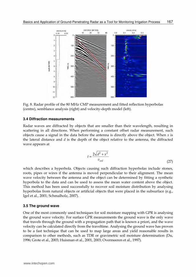
This equation describes a hyperbola, hence horizontal reflectors are mapped as reflection hyperbolas in a CMP radar section. Fig. 8 shows a CMP section from a sandy environment where the groundwater table is at 4.6 m depth. Several reflections at boundaries within the sand are visible. The first straight onset with a slope of 1/c0 is the airwave, a direct wave propagating through the air from the transmitter to the receiver. The second straight onset with a steeper slope of 1/v is the ground wave, followed by reflection hyperbolas from several reflectors in the subsurface. By fitting hyperbolas to some of the reflections, a depth-velocity model can be constructed that gives information on the water distribution. This model can also be used to transform the data from traveltimes to depth, analogous to seismic data processing (e.g., Yilmaz, 2000). When analysing multioffset data along a profile, a 2D velocity distribution of the subsurface and, thus, the water distribution can be deduced. This technique has been used successfully to map water content in the subsurface (e.g., Greaves et al., 1996; Bradford, 2008).

www.intechopen.com


167

Fig. 8. Radar profile of the 80 MHz CMP measurement and fitted reflection hyperbolas (centre), semblance analysis (right) and velocity-depth model (left).

3.4 Diffraction measurements

Radar waves are diffracted by objects that are smaller than their wavelength, resulting in scattering in all directions. When performing a constant offset radar measurement, such objects cause a signal in the data before the antenna is directly above the object. When x is the lateral distance and d is the depth of the object relative to the antenna, the diffracted wave appears at

2 22

soil

d xt

v

+=

(27)

which describes a hyperbola. Objects causing such diffraction hyperbolas include stones, roots, pipes or wires if the antenna is moved perpendicular to their alignment. The mean wave velocity between the antenna and the object can be determined by fitting a synthetic hyperbola to the data and can be used to assess the mean water content above the object. This method has been used successfully to recover soil moisture distribution by analysing hyperbolas from natural objects or artificial objects that were placed in the subsurface (e.g., Igel et al., 2001; Schmalholz, 2007).

3.5 The ground wave

One of the most commonly used techniques for soil moisture mapping with GPR is analysing the ground wave velocity. For surface GPR measurements the ground wave is the only wave that travels through the ground with a propagation path that is known a priori, and the wave velocity can be calculated directly from the traveltime. Analysing the ground wave has proven to be a fast technique that can be used to map large areas and yield reasonable results in comparison to other methods, such as TDR or gravimetric soil moisture determination (Du, 1996; Grote et al., 2003; Huisman et al., 2001, 2003; Overmeeren et al., 1997).

www.intechopen.com


168

Fig. 9. Constant offset radar section (top) over an area with natural and artificial diffracting objects (metal bars, stones, roots) and the deduced water distribution based on the fit of diffraction hyperbolas (bottom). The circles and squares indicate the positions of objects that caused the diffractions used for the analysis (with permission from Schmalholz, 2007).

There are two principle modes by which a ground wave measurement can be carried out. The first is to perform a moveout (MO, WARR) or a CMP measurement (Overmeeren et al., 1997; Huisman et al., 2001). When plotting the traveltime versus the distance to the transmitter and receiver antennas, the airwave and the ground wave onsets form a straight line whose slope corresponds to the inverse of the wave velocity in air 1/c0 and soil 1/vsoil, respectively (Fig. 10, left part, x < xopt). The extension of the air and ground wave (dashed lines in Fig. 10) intersect at the origin. The second method is to carry out a constant offset (CO) measurement by measuring lateral changes in the velocity of the ground wave (Grote et al., 2003) (Fig. 10, right part, x > xopt). In this mode, the water content distribution along a profile can be deduced rapidly. A combination of both methods was proposed by Du (1996) and is the most appropriate method to date.

Fig. 10. Schematic traveltime diagram of a ground wave measurement consisting of moveout measurements from x1 to xopt, followed by a constant offset measurement for x > xopt (aw: air wave, gw: ground wave).

www.intechopen.com


169

The ground wave technique is suited to map the water content of the topsoil over wide areas and to deduce its lateral distribution. The exact depth of investigation of the ground wave is still an object of research and is a function of antenna frequency, antenna separation and soil permittivity (e.g., Du, 1996; Galagedara et al., 2005). Fig. 11 shows an example of the result of the technique applied to a location with sandy soil that had been used as grassland. The area from x = 9 to 11 m was irrigated and shows higher water contents. TDR measurements were carried out every 20 cm along the same profile and show similar results.

Fig. 11. Water contents obtained from ground wave field measurement of a sandy soil and results of TDR measurements. The area from 9 to 11 m has been irrigated and shows higher water contents.

3.6 Reflection coefficient at the soil surface

The reflection coefficient R of an incident wave normal to an interface is described in Eq. 18.

Regarding the interface air-soil with εair = 1, we can deduce the coefficient of reflection R and, thus, the permittivity and the water content of the upper centimetres of the soil:

21

1soil

R

Rε

− =

+ (28)

This principle is also used to determine soil moisture in active remote sensing techniques over large areas (e.g., Ulaby et al., 1986). Fig. 12 shows a layout with an air-launched horn antenna mounted on a sledge so that it can be moved along profiles with a fixed distance from the soil. An example of this technique is demonstrated in Section 4.1.

3.7 Further techniques

In addition to these commonly used techniques, there are a variety of other techniques that

can be used to deduce soil-water content by means of GPR. For example, Bradford (2007)

analysed the frequency dependence of wave attenuation in the high-frequency range to

assess water content and porosity from GPR measurements. Igel et al. (2001) and Müller et

al. (2003) used guided waves that travel along a metallic rod that is lowered into a borehole.

Van der Kruk (2010) analysed the dispersion of waves that propagate in a layered soil under

certain conditions and Minet et al. (2011) used a full-waveform inversion of off-ground horn

antenna data to map the moisture distribution of a horizontally layered soil.

www.intechopen.com


170

Fig. 12. Experimental setup to determine the coefficient of reflection. A 1-GHz horn antenna is mounted on a sledge 0.5 m above the ground.

4. Application examples of GPR

In this section, two examples of GPR measurements and analyses applied for monitoring irrigation and subsequent events are given. Both examples demonstrate the ability of GPR to measure and monitor changes in the soil water content. The first example analyses reflections at the soil surface (see Section 3.6) and the second is transmission measurements between boreholes (see Section 3.1).

4.1 Monitoring of soil water content variation by GPR during infiltration

GPR measurements were carried out after irrigation to see its capability in monitoring the changes in soil dielectric properties and their spatial variation. This work demonstrates that the obtained GPR data can be used to describe the soil water distribution.

4.1.1 Experimental setup

An irrigation experiment was carried out on an outdoor test site in Hannover, Germany. The texture of the soil at the site is medium sand and the soil has a high humus content of 6.3%. The total pore volume (i.e., the maximum water capacity shortly after heavy rainfall or irrigation) of the soil is estimated to be 55 vol%. The field capacity (i.e., the maximum water content that can be stored against gravity) is approximately 21 vol%, which corresponds to a relative dielectric permittivity of 10.7 according to Topp’s equation (Topp et al., 1980). The ground surface was relatively flat.

A one-square-metre area was irrigated at a rate of approximately 12 litres per minute for approximately one hour, i.e., 720 litres of water in total. An excess of water was applied to ensure that the pore system was filled to its maximum water capacity. The relative permittivity of the soil before and immediately after the irrigation was 4 and 20.8, which corresponds to a water content of 5.5 vol% and 35.5 vol%, respectively. Because the test was carried out during the summer and there had been no rainfall for more than a half month prior to the test, the soil was assumed to be in its driest natural condition prior to the irrigation.

A frequency-domain radar system was employed and operated at a frequency range of 0.5-4.0 GHz. Antennas with a constant separation of 6 cm were fixed at a height of 5 cm

www.intechopen.com


171

above the ground surface and scanned in 1D every two minutes on an approximately 1-m-long profile with the help of a scanner. Additionally, the relative permittivity was monitored at one location off the GPR scanning line by TDR every half minute. The TDR probes are 10 cm long and were stuck vertically in the topsoil. The configuration of the measurements is illustrated in Fig. 13. The data collection was continued after the irrigation was stopped. The relative permittivity measured by TDR and soil water content at the end of the irrigation were 14 and 26 vol%, respectively (see Fig. 16).

Fig. 13. Schematic illustration of the experimental setup.

Position x [cm]

Tim

e [

ns]

(a)

20 30 40 50 60 70 80 90 100 1100

2

4

6

8

10(b)

20 30 40 50 60 70 80 90 100 110

(c)

0

2

4

6

8

10(d)

Fig. 14. Radar profiles acquired (a) before irrigation, (b) when irrigation was stopped, (c) one hour after irrigation stopped, and (d) two hours after irrigation stopped.

4.1.2 Data analysis and estimation of soil conditions

Some of the radar profiles obtained in the experiment are shown in Fig. 14. These profiles are plotted with the same colour scale. The reflections from the ground surface at 2 ns are weaker before irrigation (Fig. 14a) than after (Fig. 14b-d). This is because the reflection coefficient of the ground surface was increased by irrigation and the surface reflection became stronger. Thus, by analysing the surface reflection, it is possible to retrieve the soil water content at the soil surface as described in Section 3.5.

Fig. 15 shows waveforms acquired at the same location but at different times. The surface reflections appear at around 2 ns, but the peak amplitudes Er are different. The amplitude of the reflection is expressed with a reflection coefficient R, following Eq. 14. The reflection coefficient of an obliquely incident electromagnetic wave with an electric field parallel to the interface is given by

www.intechopen.com


172

2 1 1 2

2 1 1 2

cos cos

cos cos

Z ZR

Z Z

θ θ

θ θ

−=

+ (29)

where θ1 and θ2 are the angles of the incident and transmitted waves, respectively. The incident angle is determined by the measurement geometry. Z1 and Z2 are the intrinsic impedances of the first medium (air) and second medium (soil), respectively. The intrinsic impedance of air and incident angle are known, and the reflection amplitude was measured. Therefore, the intrinsic impedance of soil Z2, the dielectric permittivity and the water content can be calculated from the above relationships. The only unknown is the strength of the incident wave Ei, which is often measured with a metal plate with R = 1 as calibration (Serbin & Or, 2003; Igel, 2007). In this experiment, the incident wave strength was obtained using a puddle on the ground caused by the excess water supply during the irrigation. Assuming the permittivity of the water is 81, the incident wave strength can also be obtained with the above equations. If there are changes in the surface topography, the amplitude of the incident wave changes at different locations because of the antenna radiation pattern, i.e., changes in spreading loss. However, the ground surface in this experiment was almost flat, as can be seen from the traveltimes of the reflected wave in Fig. 14, which are almost constant along the profile, so the effects of topography were neglected.

Fig. 15. Waveforms sampled before irrigation (in the dry condition, labelled “initial”), when irrigation was stopped (T = 0), and one and two hours after irrigation was stopped.

The estimated dielectric permittivity from GPR data at three positions along the profile are

shown in Fig. 16 as a function of time after irrigation in comparison to the TDR measurements.

The corresponding volumetric water content is also provided on the right axis using Topp’s

equation (Topp et al., 1980). Before irrigation, the permittivity values estimated from GPR

measurements and measured by TDR are similar, but the estimated ones are slightly lower.

This is because the TDR measures permittivity averaged over the measurement volume, which

is about 10 cm deep, while the estimate using GPR is for a shallower region, perhaps a

centimetre deep. In its dry condition, the ground surface may be drier than deeper regions,

and the method could retrieve this difference. Furthermore, a lower bulk density in a

shallower region leads to a lower bulk permittivity. At the time that irrigation was stopped,

the water content measured by TDR was about 35 vol%, while the water content estimated by

GPR was higher than 50 vol%. This indicates that within very shallow soil, most of the pore

space was filled with water. After the irrigation was stopped, the measured water content

www.intechopen.com


173

slowly decreased exponentially to about 25 vol%, which is consistent with our estimate of the

field capacity. The estimated water content also decreased with time, but the decrease was

much more rapid than for the water content measured with TDR. This is also caused by the

different sampling depths of the two methods: the shallower layer mapped by GPR loses

water faster than the deeper soil horizons measured with TDR.

Fig. 16. The dielectric permittivity of the uppermost 10 cm of the soil measured by TDR (solid line) and permittivity of the ground surface estimated from GPR data, plotted as a function of time after the irrigation was stopped. Plots at the zero-time axis indicate permittivity before irrigation, i.e., the dry condition. The right axis gives the corresponding volumetric water content using Topp’s equation (Eq. 22, Topp et al., 1980).

The dielectric permittivity of the ground surface can also be estimated depending on the position along the profile. The left side of Fig. 17 shows the spatial variation in permittivity and water content at different times as a function of the position. The water content, as well as its spatial variation, were not high in the dry condition, but both were increased by irrigation. The spatial distributions before and after irrigation are similar but not exactly the same. As shown in Fig. 16, most of the decrease in water content in the shallow region occurred within the first 30 minutes, and the calculated spatial water distribution at one and two hours after irrigation ceased are almost the same.

Fig. 17. Left: the spatial variation in dielectric permittivity of the ground surface estimated from GPR data. Right: the standard deviation of the estimated relative permittivity in space. The cross at time zero indicates the value before irrigation.

www.intechopen.com


174

By further analysing the spatial variation of dielectric permittivity and water content, the soil water distribution can be understood. The right side of Fig. 17 shows the standard deviation of permittivity plotted as a function of time. The variation was very small for the dry condition. By adding water, the variation increased and continued to increase for about 10 minutes after irrigation was stopped. It then decreased and became stable but was still higher than for the dry condition. The result can be interpreted as water that had infiltrated and percolated into the ground during and shortly after irrigation, but the percolation velocity varies spatially on a small scale, depending on differences in bulk density, texture, humus content and related pore volume, i.e., water was drained faster in areas with higher proportions of transmission pores. The variation in percolation velocity caused a variation in water content and an increase in the standard deviation of permittivity for a short period of time after irrigation was stopped. Areas with a smaller pore volume may have stored more water than their field capacity for a short time, but the excess water subsequently percolated out. This behaviour led to a decrease in variation in permittivity. After some time, all sections stored as much water as the field capacity and the variation became stable, but remained higher than at the dry condition.

4.2 Infiltration monitoring by borehole GPR

An artificial groundwater recharge test was carried out in Nagaoka City, Japan (Kuroda et

al., 2009). Time-lapse cross-hole measurements were performed at the same time to monitor

the infiltration process in the vadose zone.

4.2.1 Field experiment

The borehole GPR measurement carried out during the infiltration experiment is

schematically illustrated in Fig. 18. The top 2 m of soil consisted of loam, and the subsoil

was sand and gravel. The groundwater table was located approximately 10 m below the

ground surface. During the experiment, water was injected from a 2 x 2 m tank with its base

set at a depth of 2.3 m. The total volume of water injected into the soil was 2 m3, requiring

approximately 40 minutes for all water to flow from the tank. Two boreholes were located

on both sides of the tank with a separation of 3.58 m. Using these boreholes, GPR data were

acquired in a ZOP configuration. In this mode, both the transmitter and receiver antennas

were lowered to a common depth. Data were collected every 0.1 m at depths of 2.3-5.0 m.

This required about 2 minutes to cover the whole depth range. A total of 25 profiles were

obtained during the experiment, which lasted 322 minutes.

4.2.2 Estimation of percolation velocity

Three radar profiles acquired from this experiment are shown in Fig. 19. The first arrival

times range from 36-38 ns in the initial, unsaturated state (Fig. 19a), and 42-44 ns in the final

state (Fig. 19c), which is considered to be fully saturated. In the intermediate state of 51-53

minutes after infiltration, the first arrival times are almost identical to the initial state at

depths below 4 m (Fig. 19b). Shallower than 4 m depth, the first arrival times are delayed:

the shallower the depth, the greater the traveltime. This delay is caused by increased

wetting in the vadose zone (transition zone).

www.intechopen.com


175

Fig. 18. Schematic sketch of the artificial ground water recharge test in the vadose zone.

Fig. 19. Radar profiles observed during the infiltration test: (a) before infiltration, (b) 52 min

after infiltration, and (c) 106 min after infiltration. Triangles show the picked first arrival

times.

The infiltration process may not be 1D because the vadose zone is heterogeneous. Since the standard ZOP method relies on determining the velocity of an electromagnetic wave that follows a straight path from the transmitter to the receiver, the infiltration process is assumed to be 1D. Fig. 20 shows vertical profiles of the first arrival times. In these profiles, the volumetric water content at a specific depth is estimated based on the following procedure. By assuming a straight raypath, a first arrival time is used to calculate the velocity v using v = d/t, where d is the offset distance between the transmitter and the receiver, and t is the traveltime. By assuming that frequency-dependent dielectric loss is

small (Davis and Annan, 1989), the apparent dielectric constant ε is obtained using Eq. 2.

Finally, the volumetric water content θ can be estimated by substituting ε into the empirical Topp’s equation (Eq. 22, Topp et al., 1980).

The spatial and temporal variations of volumetric water content are derived using all first arrival times collected during the infiltration experiment (Fig. 21). This illustration clearly shows the movement of the wetting front in the test zone during the infiltration process. The water content varies sharply from the unsaturated state (lower left side) to the saturated

www.intechopen.com


176

state (upper right side). The zone exhibiting significant changes can be interpreted as a transition zone. The average downward velocity of percolating water in the test zone is estimated to be about 2.7 m/h and is the boundary between the unsaturated and transition zones (Fig. 21).

Fig. 20. First arrival times picked from the time-lapse ZOP radar profiles at three different conditions of the infiltration experiment. EM-wave velocities estimated using first arrival times are transformed into apparent dielectric constants and further converted into volumetric water contents.

Fig. 21. A map showing the spatiotemporal variations in volumetric water content in the test

zone during the infiltration process. The infiltrated water penetrated vertically with a

velocity of about 2.7 m/h.

5. Conclusion

In this chapter, the basics of GPR and the principles for measuring soil water content are

discussed. Two examples are given where GPR was used to monitor the temporal changes

in soil water content following irrigation. The first example describes analysis of the

reflection amplitude of electromagnetic waves, which depends on the dielectric permittivity

www.intechopen.com


177

and the water content of soil. This technique is very fast and can be used to obtain results

with a very high spatial and temporal resolution. The second example utilised the fact that

the velocity of the electromagnetic waves is determined by the dielectric permittivity and

the water content of soil. Although this method requires boreholes to carry out a

transillumination measurement, it can capture vertical changes in soil water content. These

examples clearly demonstrated the capability of GPR to measure water-related soil

properties. Compared to other methods for the measurement of soil water content, GPR can

measure a larger area easily and quickly with a high spatial and temporal resolution. As

shown in Section 3, there are a variety of techniques to measure or estimate the soil water

content. Most of them are completely non-invasive, which is a very important feature for

monitoring soil water content at the same location. One can chose the most suitable method

according to the possible measurement setup and the desired type of result. Therefore, GPR

has a great potential for use in investigations of irrigation and soil science.

6. List of symbols

c Velocity of light in free space m/s d Depth m f Frequency Hz k Wavenumber 1/m t Time s

tanδ Loss tangent v Propagation velocity of electromagnetic waves m/s E Electric field strength of an electromagnetic wave V/m E0 Original electric field strength of an electromagnetic field V/m Ei Incident electric field strength V/m Er Reflected electric field strength V/m Et Transmitted electric field strength V/m R Reflection coefficient Sw Water saturation T Transmission coefficient

Z Intrinsic impedance Ω

α Attenuation constant Np/m

α’ Attenuation constant dB/m

β Phase constant 1/m

δ Skin depth m

ε Absolute dielectric permittivity F/m

ε’ Real part of dielectric permittivity F/m

ε” Imaginary part of dielectric permittivity F/m

ε0 Absolute dielectric permittivity of free space F/m

εe Complex effective permittivity F/m

εr Relative dielectric permittivity

εs Low frequency static permittivity F/m

ε∞ High frequency permittivity F/m

φ Porosity

λ Wavelength m

www.intechopen.com


178

µ Absolute magnetic permeability H/m

µ0 Absolute magnetic permeability of free space H/m

µr Relative magnetic permittivity

θv Volumetric water content

σ Electric conductivity S/m

σ’ Real part of electric conductivity S/m

σ” Imaginary part of electric permittivity S/m

σq Interface conductivity S/m

τ Relaxation time s

ω Angular frequency rad/s

7. References

Annan, A.P. (2005). Ground penetrating radar in near-surface geophysics, In: Near-Surface Geophysics, Investigations in Geophysics, No. 13, Society of Exploration Geophysics, Butler, D.K., pp.357-438, ISBN 1-56080-130-1, Tulsa, OK

Annan, A.P. (2009). Electromagnetic principles of ground penetrating radar, In: Ground Penetrating Radar: Theory and Applications, Jol, H.M., pp. 3-40, Elsevier, ISBN 978-0-444-53348-7, Amsterdam, The Netherlands

Archie, G.E. (1942). The electrical resistivity log as an aid in determining some reservoir characteristics. Petroleum Transactions of AIME, Vol. 146, pp. 54-62

Binley, A., Winship, P., Middleton, R., Pokar, M. & West, J. (2001). High-resolution characterization of vadose zone dynamics using cross-borehole radar. Water Resources Research, Vol. 37, pp. 2639-2652

Bradford, J.H. (2007). Frequency-dependent attenuation analysis of ground-penetrating radar data. Geophysics, Vol. 72, pp. J7-J16

Bradford, J.H. (2008). Measuring water content heterogeneity using multifold GPR with reflection tomography. Vadose Zone Journal, Vol. 7, pp. 184-193

Cassidy, N.J. (2009). Electrical and magnetic properties of rocks, soils, and fluids, In: Ground Penetrating Radar: Theory and Applications, Jol, H.M., pp. 41-72, Elsevier, ISBN 978-0-444-53348-7, Amsterdam, The Netherlands

Daniels, D.J. (Ed.). (2004). Ground Penetrating Radar (2nd Edition), IEE, ISBN 0-86341-360-9, London

Davis, J.L. & Annan, A.P. (1989). Ground-penetrating radar for high resolution mapping of soil and rock stratigraphy. Geophysical Prospecting, Vol. 37, pp. 531-551

Dix, C.H. (1955). Seismic velocities from surface measurements. Geophysics, Vol. 20, pp. 68-86

Du, S. (1996). Determination of Water Content in the Subsurface with the Ground Wave of Ground Penetrating Radar. Dissertation, Ludwig-Maximilians-Universität, München, Germany

Galagedara, L.W., Redman, J.D., Parkin, G.W., Annan, A.P. & Endres, A.L. (2005). Numerical modeling of GPR to determine the direct ground wave sampling depth. Vadose Zone Journal, Vol. 4, pp. 1096-1106

Greaves, R.J., Lesmes, D.P., Lee, J.M. & Toksoz, M.N. (1996). Velocity variations and water content estimated from multi-offset ground penetrating radar, Geophysics, Vol. 61, pp. 683-695

www.intechopen.com


179

Grote, K., Hubbard, S. & Rubin, Y. (2003). Field-scale estimation of volumetric water content using ground-penetrating radar ground wave techniques. Water Resources Research, Vol. 39, pp. 1321-1333

Huisman, J.A., Sperl, C., Bouten, W. & Verstaten, J.M. (2001). Soil water content measurements at different scales: accuracy of time domain reflectometry and ground-penetrating radar. Journal of Hydrology, Vol. 245, pp. 48-58

Huisman, J.A., Hubbard, S.S., Redman, J.D. & Annan, A.P. (2003). Measuring soil water content with ground penetrating radar: a review. Vadose Zone Journal, Vol. 2, pp. 476-491

Igel, J., Schmalholz, J., Anschütz, H.R., Wilhelm, H., Breh, W., Hötzl, H. & Hübner C. (2001). Methods for determining soil moisture with the ground penetrating radar (GPR). Proceedings of the Fourth International Conference on Electromagnetic Wave Interaction with Water and Moist Substances, Weimar, Germany.

Igel, J. (2007). On the Small-Scale Variability of Electrical Soil Properties and Its Influence on Geophysical Measurements. PhD Thesis, Johann Wolfgang Goethe-Universität, Frankfurt am Main, Germany

Kaatze, U. (1989). Complex permittivity of water as a function of frequency and temperature. Journal of Chemical and Engineering Data, Vol. 34, pp. 371-374

Knight, R.J. & Endres, A.L. (2005). An introduction to rock physics principles for near-surface geophysics, In: Near-Surface Geophysics, Investigations in Geophysics, No. 13, Society of Exploration Geophysics, Butler, D.K., pp.357-438, ISBN 1-56080-130-1, Tulsa, OK

Knödel, K., Lange, G., & Voigt, H.-J. (Eds.). (2007). Environmental Geology, Handbook of Field Methods and Case Studies, Springer, ISBN 978-3-540-74669-0, Berlin

Kuroda, S., Jang, H. & Kim, H.J. (2009). Time-lapse borehole radar monitoring of an infiltration experiment in the vadose zone. Journal of Applied Geophysics, Vol. 67, pp. 361-366

Lampe, B. & Holliger, K. (2003). Effects of fractal fluctuations in topographic relief, permittivity and conductivity on ground-penetrating radar antenna radiation. Geophysics, Vol. 68, pp. 1934-1944

Minet, J., Wahyudi, A., Bogaert, P., Vanclooster, M., & Lambot, S. (2011). Mapping shallow soil moisture profiles at the field scale using full-waveform. Geoderma, Vol. 161, pp. 225-237

Müller, M., Mohnke, O., Schmalholz, J. & Yaramanci, U. (2003). Moisture assessment with small-scale geophysics - the Interurban project. Near Surface Geophysics, Vol. 1, pp. 173-181

Noborio, K. (2001). Measurement of soil water content and electrical conductivity by time domainreflectometry: a review. Computers and electronics in agriculture, Vol. 31, 213-237

Overmeeren, R.A., Sariowan, S.V. & Gehrels, J.C. (1997). Ground penetrating radar for determining volumetric soil water content; results of comparative measurements at two test sites. Journal of Hydrology, Vol. 197, pp. 316-338

Preetz, H., Altfelder, S. & Igel, J. (2008). Tropical soils and landmine detection – an approach for a classification system. Soil Science Society of America Journal, Vol. 72, pp. 151-159

www.intechopen.com


180

Robinson, D.A., Jones, S.B., Wraith, J.M., Or, D. & Friedmann, S.P. (2003). A review of advances in dielectric and electrical conductivity measurement in soils using time domain reflectometry. Vadose Zone Journal, Vol. 2, pp. 444-475

Schmalholz, J., Stoffregen, H., Kemna, A. & Yaramanci, U. (2004). Imaging of Water Content Distributions inside a Lysimeter using GPR Tomography. Vadose Zone Journal, Vol. 3, pp. 1106-1115

Schmalholz, J. (2007). Georadar for small-scale high-resolution dielectric property and water content determination of soils. Dissertation, Technical University of Berlin, Germany

Serbin, G. & Or, D. (2003). Near-surface soil water content measurements using horn antenna radar: methodology and overview. Vadose Zone Journal, Vol. 2, pp. 500-510

Shen, L.C., Savre, W.C., Price, J.M. & Athavale, K. (1985). Dielectric properties of reservoir rocks at ultra-high frequencies, Geophysics, Vol. 50, pp. 692-704

Stoffregen, H., Zenker, T., Wessolek, G. (2002). Accuracy of soil water content measurements using ground penetrating radar: Comparison of ground penetrating radar and lysimeter data. Journal of Hydrology, Vol. 267, pp. 201-206

Takahashi, K., Preetz, H. & Igel, J. (2011). Soil properties and performance of landmine detection by metal detector and ground-penetrating radar – Soil characterisation and its verification by a field test. Journal of Applied Geophysics, Vol. 73, pp. 368-377

Topp, G.C., Davis, J.L. & Annan, A.P. (1980). Electromagnetic determination of soil water content: measurements in coaxial transmission lines. Water Resource Research, Vol. 16, pp.574-582

Tronicke, J., Tweeton, D.R., Dietrich, P. & Appel, E. (2001). Improved crosshole radar tomography by using direct and reflected arrival times. Journal of Applied Geophysics, Vol. 47, pp. 97-105

Ulaby, F.T., Moore, R.K. & Adrian, K.F. (1986). Microwave Remote Sensing: Active and Passive, volume 3: From Theory to Applications. Artech House, ISBN 0-89006-192-0, Norwood, MA

van der Kruk, J., Jacob, R.W. & Vereecken, H. (2010). Properties of precipitation-induced multilayer surface waveguides derived from inversion of dispersive TE and TM GPR data. Geophysics, Vol. 75, pp. WA263-WA273

Yilmaz, O. (2000). Seismic data analysis - processing, inversion, and interpretation of seismic data (2nd edition). Society of Exploration Geophysicists, ISBN 978-0931830464, Tulsa, OK

www.intechopen.com

Problems, Perspectives and Challenges of Agricultural WaterManagementEdited by Dr. Manish Kumar

ISBN 978-953-51-0117-8Hard cover, 456 pagesPublisher InTechPublished online 09, March, 2012Published in print edition March, 2012

InTech EuropeUniversity Campus STeP Ri Slavka Krautzeka 83/A 51000 Rijeka, Croatia Phone: +385 (51) 770 447 Fax: +385 (51) 686 166www.intechopen.com

InTech ChinaUnit 405, Office Block, Hotel Equatorial Shanghai No.65, Yan An Road (West), Shanghai, 200040, China

Phone: +86-21-62489820 Fax: +86-21-62489821

Food security emerged as an issue in the first decade of the 21st Century, questioning the sustainability of thehuman race, which is inevitably related directly to the agricultural water management that has multifaceteddimensions and requires interdisciplinary expertise in order to be dealt with. The purpose of this book is tobring together and integrate the subject matter that deals with the equity, profitability and irrigation waterpricing; modelling, monitoring and assessment techniques; sustainable irrigation development andmanagement, and strategies for irrigation water supply and conservation in a single text. The book is dividedinto four sections and is intended to be a comprehensive reference for students, professionals andresearchers working on various aspects of agricultural water management. The book seeks its impact from thediverse nature of content revealing situations from different continents (Australia, USA, Asia, Europe andAfrica). Various case studies have been discussed in the chapters to present a general scenario of theproblem, perspective and challenges of irrigation water use.

How to referenceIn order to correctly reference this scholarly work, feel free to copy and paste the following:

Kazunori Takahashi, Jan Igel, Holger Preetz and Seiichiro Kuroda (2012). Basics and Application of Ground-Penetrating Radar as a Tool for Monitoring Irrigation Process, Problems, Perspectives and Challenges ofAgricultural Water Management, Dr. Manish Kumar (Ed.), ISBN: 978-953-51-0117-8, InTech, Available from:http://www.intechopen.com/books/problems-perspectives-and-challenges-of-agricultural-water-management/basics-and-application-of-ground-penetrating-radar-as-a-tool-for-monitoring-irrigation-process

basics and application of ground- penetrating radar as a...

Documents