basics and magnetic materials - magnetism.eu - ema - the european magnetism...

BASICS AND MAGNETIC MATERIALSK.-H. Müller

Institut für Festkörper- und Werkstoffforschung Dresden,POB 270116, D-01171 Dresden, Germany

1 – INTRODUCTION

2 – MAGNETIC MOMENT AND MAGNETIZATION

3 – LOCALIZED ELECTRON MAGNETISM

4 – ANISOTROPY AND DIMENSIONALITY

5 – PHASE TRANSITIONS AND MAGNETIZATION PROCESSES

History of magnetism• the names magnetism, magnets etc. go back to ancient Greeks:

magnetite = loadstone (Fe3O4)

• The magnetism of magnetite was also known in ancient China

- spoon-shaped compass 2000 years ago

- long time used for geomancy

- open-see navigation since 1100

European traditions in magnetism• A. Neckham (1190): describes the compass

• P. Peregrinus (1269): Epistola Petri Peregrini … de Magnete- terrella, poles

• E.W. Gilbert (1544 – 1603)de Magnete

• R. Descartes (1569 – 1650)divorced physics from metaphysics

Modern developments in the 19th century

H.C. Oersted (1777-1851)• electric currents are magnets

J.C. Maxwell (1831-1871)• unification of light, electricity, magnetism• j → j + ε0• prediction of radio waves

A.M. Ampère (1755-1836)• ∇ x H = j• molecular currents

M. Faraday (1791-1867)• magnetic field• ∇ x E = -

H.A. Lorentz (1853-1928)•• Lorentz transformation

B&

E&)( xBvEv += em&

The revolutionary 20th century

P. Curie (1859-1906)• paramagnetism and ferromagnetism

N. Bohr, W. Heisenberg, W. Pauli• quantum theory• the need of spin

P. Dirac• relativistic quantum theory• explains the spin

P. Weiss• the molecular field• domains

→ exchange interaction ←

Magnetism and magnetic materials in our daily life

• earth's field

• natural electromagnetic waves

• TV

• portable phone

• telecommunication

• home devices

• 50 permanent magnets inan average home

• up to 100 permanent magnetsin a modern car

• soft magnetic materials inpower stations and motors and high frequency devices

• traffic

• medicine

• information technology

all magnetic materialstotal 30B$

permanent magnet materials

others

ferrites 55%Nd-Fe-B30%

permanent magnets20%

soft magnets27%

magnetic recording53%

Magnet materials – world market- in the late 20th century -

Brain ; Intergalactic space 10-13

Heart 10-10

Galaxy 10-9

urbanic noise 10-6…10-8

Surface of earth 5·10-5

near power cable (in home) 10-4

Surface of sun 10-2

surface of magnetite 5·10-1 simple resistive coil 10-1

permanent magnets 1supercond. permanent magnets 16superconducting coils 20high performance resistive coils (stationary)

26

hybrid magnets (resistive + supercond.) 40long pulse coil (100ms) 60short pulse coil (10 ms) 80

Anisotropy fields in solids ≤ 102 one-winding coil 3·102

Exchange fields in solids ≤ 103 explosive flux compression 3·103

Neutron stars 108

Fields in nature, engineering and sciencein Tesla

2 – Magnetic moment and magnetization2-1 Magnetization in Maxwell's equations

microscopic form of Maxwell's equ.ieh +ε=∇ &0x

he &0µ−=∇ x

0=∇hr0 =ε∇ e

0r =∇+ i&

⇒ jPeMh ++ε=−∇ &&0)(x ρ=+ε∇ )( Pe0

macroscopic form of Maxwell's equ.jDH +=∇ &x 0=∇ BHE &

0µ−=∇ x ρ=∇ D0=∇+ρ j

macroscopic fields 0µ≡ /BhEe =

MBH −µ≡ 0/PED +ε≡ 0

⇒⇒

magnetic moment and magnetization

∫∫ τ==∇τ−≡⇒−∇=∇VV

MdMrmMH Kd ⇒

⇒ M is a density of magnetic moments ≡ "magnetization"

P∇−ρ=rPMji &+∇+= x

magnetization M and polarization P

2-2 Magnetic moment and angular momentum

∫∫ ∇τ==∇τ−=VV

)()( xx MrMrm d21d K

⇒ LLvrmm e

m e

m e

2g

2d

2 m ==ρτ= ∫Vx

A. Einstein and W.J. de Haas (1915): g ≈ 2 (instead of 1)

G. Uhlenbeck and S. Goudsmit (1925): atomic spectra at B ≠ 0 (Zeeman effect)

spin of the electron: S → ±ħ/2 g = 2

The spin of the electron and its g-factor

scale

mirror

iron bar

A. Einstein and W.J. de Haas (1915) W. Gerlach and O. Stern (1922)

z∂B/∂z ≠ 0

Ag atoms

2-3 Quantization and relativity; diamagnetismH.A. Lorentz )( xBvEv += em&

Dirac's Hamiltonian ))()( SLBSL (λ−+++−= 222

0 yx4

B2

22 m

em e 2

HH

⇒ m = <µ > = – ∂< H >/∂B M = N <µ >

χij = µ0∂Mi/ ∂Bj = – µ0N ∂2< H >/∂Bi∂Bj

diamagnetic susceptibility (in 10-6): H2O: –9, alcohol: –7.2

Omnipresence of diamagnetism

Ho2@C84 in a glass ampouleT = 1.8 K

0 1 2 3 4 5 6 7 80.0

0.1

0.2

0.3

0.4

0.5

0.6

0.7

0.8

0.9

Mag

netiz

atio

n (a

.u.)

Magnetic field (T)

Brillouin function

• µ0H ≈ 23 Tesla

• F ∼ χ ·H · (dH/dz)

• stable only for χ < 0

Levitation of a diamagnetic body

M. Kitamura et al., Jpn. J. Appl. Phys. 39 (2000) L324

levitated glass cube melted by a laser beam

Stable position of a superconducting permanent magnet

Levitation Cross stiffnessSuspension

• by varying the spatial distribution of the external field the position of the superconducting magnet may have different degrees of freedom :

0 D – as in the examples above 1 D – as a train on a rail

• the same holds for rotational degrees of freedom

YBCO

NdFeB

2-4 Magnetization in thermodynamicsproblems:

(i) thermodynamically metastable states

(ii) the field generated by the samples own magnetization

(iii) how to define a correct expression for magnetic work

• Quantum statistical thermodynamics with the Hamiltonian H

• alternative definition of internal energy

U = < H > + µ0 Hm (a Legendre transformation)

(iv) magnetostatic interaction is long range

⇒

⇒ both expressions are correct: work done on different systems !

∫ τµ+δ=µ+δ=V

MHmH ddQdQdU 00

∫ τµ−δ=µ−δ=><V

HMHm ddQdQd 00H

1H

2He

3Li

4Be

5B

6C

7N

8O

9F

10Ne

11Na

12Mg

13Al

14Si

15P

16S

17Cl

18Ar

19K

20Ca

21Sc

22Ti

23V

24Cr

25Mn

26Fe

27Co

28Ni

29Cu

30Zn

31Ga

32Ge

33As

34Se

35Br

36Kr

37Rb

38Sr

39Y

40Zr

41Nb

42Mo

43Tc

44Ru

45Rh

46Pd

47Ag

48Cd

49In

50Sn

51Sb

52Te

53I

54Xe

55Cs

56Ba

72Hf

73Ta

74W

75Re

76Os

77Ir

78Pt

79Au

80Hg

81Tl

82Pb

83Bi

84Po

85At

86Rn

Periodic System of Elements

57La

58Ce

59Pr

60Nd

61Pm

62Sm

63Eu

64Gd

65Tb

66Dy

67Ho

68Er

69Tm

70Yb

71Lu

Magnetism in atoms and condensed matter

2-5 Localized vs. itinerant electron magnetism in solids• isolated atoms or ions with incompletely filled electron shells

• magnetization: M ∼ BJ(H/T)

⇒ Curie's law M = χ H with χ = C/T

• Two main types of solids– large electron density ⇒ delocalized (itinerant) electrons – e.g. in Li- or Na-metal

⇒ Hund's rule magnetic moment disappears⇒ a small, (nearly) temperature independent susceptibility

– small electron densities⇒ strongly correlated electrons⇒ they can be localized and carry a magnetic moment⇒ examples: MnO, FeO, CoO, CuO (antiferromagnets); EuO, CrCl3 (ferromagnets)

• In 4f materials localized and itinerant electrons coexist

2-6 Itinerant electron magnetism

• weakly interacting Landau quasiparticles

)*

()( 2

2

F2B0 3

11E2mmN −µµ=χ with m

e2Bh||

=µ

⇒ metals with large or moderate m* (e.g. Na: m/m* ≈ 1)are Pauli paramagnets, χ > 0

⇒ those with small m* (e.g. Bi m/m* ≈ 102)are Landau diamagnets, χ < 0

Susceptibility vs. temperatureafter M. Bozort 1951

MO

LEC

ULA

R S

USC

EPTI

BIL

ITY

TEMPERATURE [°C]-200 8006004002000

10-3

10-4

10-5

10-6

-10-6

-10-5

-10-4

-10-3

Itinerant electron magnetism

• large fields and low temperatures

⇒ discrete Landau levels:

⇒ de Haas-van Alphen effect, Shubnikov-de Haas effect

⇒ an oscillation of M(H)

*2)k(H1/2)(nE

2z0

n mme h

h +µ

+=*|| with H || z

0.04 0.08 0.12 0.16 0.20-0.3

-0.2

-0.1

0.0

0.1

0.2

0.3

Applied field µ0H (T)

CeBiPtH II [100]

25 510

σ xx

1/(µ0H) (1/T)

50

T = 4.2 K

Shubnikov-de Haas effect in CeBiPt

Itinerant electron magnetism

• Slater (1936) and Stoner (1938) the interaction between itinerant electrons

][MMcM)(EI1)(E4

1E 642F

F2B

0 ONN

++−µ

+µ−= )(MH

⇒ finite value of M, even for H = 0, if I N(EF) > 1 (Stoner condition)

• IN(EF) < 1 ⇒ the paramagnetic state remains stable ⇒ exchange enhancement

)(EI1)(E2

F

F2B0

NN

−µµ

=χ

• itinerant antiferromagnetism and spin density waves (by χ0(Q))

⇒ modified theory of spin fluctuations (T. Moriya 1978)⇒ e.g. the afm in Cr

⇒ e.g. in Pd

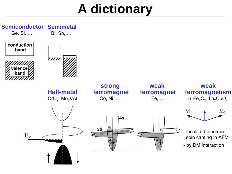
A dictionarySemiconductor

Ge, Si, …Semimetal

Bi, Sb, …

valenceband

conductionband

Half-metalCrO2, Mn2VAl

EF

weak ferromagnet

Fe, …

weakferromagnetism

α-Fe2O3, La2CuO4

M1 M2

- localized electron spin canting in AFM

- by DM interaction

4s

3d

strongferromagnet

Co, Ni, …

4s

3d

• electrons of partially filled shells: localized by correlation ⇒ carrying a magnetic moment

• mostly from 3d or 4f electrons in alloys and compounds ⇒ ⇒ ⇒

3 – Localized electron magnetism

susc

eptib

ility

temperature (K)

χ

1/χ

CuSO4·5H2O


• mostly from 3d or 4f electrons in alloys and compounds


• also 5f or 2p⇒ solid O2 – an AFM: TN ≈ 30K⇒ TDAE-C60 – an organic FM ⇒

TDAE ≡ C2N4(CH3)8

TcTemperature (K)

Mag

netiz

atio

n (m

T)TDAE-C60


• mostly from 3d or 4f electrons in alloys and compounds


• also 5f or 2p⇒ solid O2 (Ts = 54K) – an antiferromagnet: TN = (25…40)K⇒ TDAE-C60 – an organic ferromagnet

TDAE ≡ C2N4(CH3)8

• interactions:⇒ total quenching of <L> ⇒ ML = 0

⇒ cooperative phenomena of magnetic ordering

3-1 Effects of crystalline electric fields (CEF)• atomic cores on the neighbour sites ⇒ electrostatic potential

⇒ no rotational symmetry ⇒ Lz no good quantum number ⇒ Lz-mixing : Lz/ħ = +2, -2 ⇒ dx2-y2

• formalism of K.H.W. Stevens (1952)• contribution L to M reduced or even totally "quenched"

++–

–

number of 3d -electrons

mag

netic

mom

ent

[ µB

]

Cr++

L-quenching in salts in two-valent 3d ions

spin-only value

Hund's rule(free ion) values

J = L ± S

• the experimental values (x) are close to the spin only values• e.g. Cr++ : L /ħ = 2 +1 +0 + (-1) = 2 , S/ħ = 4x1/2 = 2 , J = L – S = 0

h/)1(2 BSS µµ +=

Mn++

Effects of crystalline electric fields (CEF)

• if CEF-splitting >> Hund's-rule interaction⇒ "High-spin–low-spin transition" or "spin quenching"

e.g. Fe++ in octahedral anionic environments

∆(CEF) < ∆(HR)⇒ S = 2ħ (high spin)

Hund's rule value∆(CEF) > ∆(HR)

⇒ S = 0 (low spin)

eg

t2g

• atomic cores on the neighbour sites ⇒ electrostatic potential⇒ no rotational symmetry ⇒ Lz no good quantum number ⇒ Lz-mixing : Lz/ħ= +2, -2 ⇒ dx2-y2

• formalism of K.H.W. Stevens (1952)• contribution L to M reduced or even totally "quenched"

++–

–

The ferromagnetic cuprate La2BaCuIIO5F. Mizuno et al., Nature 345 (1990) 788

d(Cu-O) ≈ 1.92Åa-b planeP4/mbm

c

Ba

O

La

ca

a

Cu

• CuO4 plaquettes as typical for CuII cuprates

• the plaquettes are nearly isolated ⇒ d ≈ 0

• µp ≈ 1.8 µB ; µs ≈ 1 µB ⇒ S = ħ/2

• Tc ≈ 6 K ;

• ⇒ magnetic coupling between the CuII spins

• relatively strong magnetic anisotropy Magnetic field (Oe)0 200 400 600

2

4

6

8

H ⊥ cH || c

T = 2KM

agne

tizat

ion

[em

u/g]

• spin orbit interaction is magnetic in its nature

• governs the third Hund's rule

• opposes L quenching ⇒ e.g. in 4f-elements, alloys, compounds : J = L ± S

⇒ zero field splitting (simplest case): , J/ħ integral ⇒ Jz = 0

))()( SLBSL (λ−+++−= 222

0 yx4

B2

22 m

em e 2

HH

3-2 Spin orbit interaction and CEF

• H mixes the ground state singlet of non-Kramers ions with excited CEF states ⇒ Van Vleck paramagnetism

• H.A. Kramers (1930): odd number of electrons ⇒ even degeneracy

⇒ "Kramers ions" (e.g. Cu++, Nd3+) ⇒ "non-Kramers ions" (even numbers of electrons as in Fe++, Pr3+)

⇒ singlets possible

2zJD~CEF =H

Behaviour of Kramers and non-Kramers ions

χ-1

[a.u

.]

temperature temperature

χ-1

[a.u

.]

10 energy levels

• non-Kramers ion Pr3+ : 2 electronsS = ħ, L = 5ħ , J = 4ħ

χ(T→0) finite⇒ Van Vleck paramagnetism

• Kramers ion Nd3+ : 3 electronsS = 3ħ/2, L = 6ħ, J = 9ħ/2

χ(T→0) → ∞⇒ Curie-Langevin paramagnetism

Pr2(SO4)3·8H2O Nd2(SO4)3·8H2O

• spin orbit interaction is magnetic in its nature

• governs the third Hund's rule

• opposes L quenching ⇒ e.g. in 4f-elements, alloys, compounds : J = L ± S

⇒ zero field splitting (simplest case): , J/ħ integral ⇒ Jz = 0

))()( SLBSL (λ−+++−= 222

0 yx4

B2

22 m

em e 2

HH

Spin orbit interaction and CEF

• H mixes the ground state singlet of non-Kramers ions with excited CEF states ⇒ Van Vleck paramagnetism

• H.A. Kramers (1930): odd number of electrons ⇒ even degeneracy

⇒ "Kramers ions" (e.g. Cu++, Nd3+) ⇒ "non-Kramers ions" (even numbers of electrons as in Fe++, Pr3+)

⇒ singlets possible

2zJD~CEF =H

•S-L-interaction mediates magnetic anisotropy from the lattice to the spin (or to J)

3-3 Dipolar interaction

5ji

2ji

0dip r43r

j)(i,Eπ

−µ=

)()()( rmrmmm

⇒ is omnipresent in magnetic materials⇒ results in magnetic ordering temperatures of typically 1 K⇒ is long range ⇒ anisotropic

• interaction energy of two dipoles mi, mj

• self-energy of a magnetization M(r) in volume V

H'(r)M(r)τµ

−= ∫Vd

2E 0

self

- is only semiconvergent - in homogenously magnetized samples, M(r) = M = const

∑µ=

ji, jiji,0

self MMDV2

E ∑ =i i 1D Di ≥ 0 demagnetization factors

⇒ "demagnetizing fields" <H'i(r)>V = – Di M (bodies of arbitrary shape!)

with ,)()(' rMrH ∇−=∇ 0=∇ )('x rH

Examples of demagnetizing fields

H'

M

sphere D =1/3

H' = – M/3

hollow sphere D =1/3

H'=0M

H' = 0

H' = –M

<H'> = – M/3

cube D = 1/3

<H'> = – M/3

H'(r)non-uniform

prolate spheroid

M

D = 0 ⇒ H' = 0

prolate spheroid

M

D = 1/2 ⇒ H' = –M/2

long cylinder

MH' = –M/2

H' = M/2D = 0 ⇒ <H'> = 0

Dipolar interaction

5ji

2ji

0dip r43r

j)(i,Eπ

−µ=

)()()( rmrmmm

⇒ is omnipresent in magnetic materials⇒ results in magnetic ordering temperatures of typically 1 K⇒ is long range

• self-energy of a magnetization M(r) in volume V

H'(r)M(r)τµ

−= ∫Vd

2E 0

self

- is only semiconvergent - in homogenously magnetized samples, M(r) = M = const

∑µ=

ji, jiji,0

self MMDV2

E ∑ =i i 1D Di ≥ 0 demagnetization factors

⇒ "demagnetizing fields" <H'i(r)>V = – Di M (bodies of arbitrary shape!)

• interaction energy of two dipoles mi, mj

with

⇒ tensor character of (Di,j) ⇒ shape anisotropy

,)()(' rMrH ∇−=∇ 0=∇ )('x rH

Effects of dipole-dipole interaction5ij

ijjiji2ijji

0dip r43r

j)(i,Eπ

−µ=

)()()( rmrmmm

• is magnetic in its nature and anisotropic

⇒ its effect is sensitive to to the presence of other interactions

1.) two dipoles governed by Edip only ⇒ or

2.) if additionally m1 || m2 required (strong exchange interaction)

typical easy-axis magnetic anisotropy)( ϑ−π

µ= 2

3ij

20

dip 31r4

mE cosϑ

rij

rij rij

3.) if the dipoles are confined to a certain axis (by strong CEF)

antiferromagneticalignment

ferromagneticalignment

a) b)axis axisrijrij

3-4 Exchange interaction

wave function antisymmetric in r1 and r2

symmetric in r1 and r2

energy difference at R0 : Eant – Esymm ≡ -J

• the Pauli principle requires antisymetric total wave functions

• spin space Ψ(s=0) = {(χ1(↑) χ2(↓) – χ1(↓) χ2(↑)}/√2

s = s1 + s2 Ψ(s=1, sz=1) = (χ1(↑) χ2(↑)si =1/2 Ψ(s=1, sz=0) = {(χ1(↑) χ2(↓) + χ1(↓) χ2(↑)}/√2

(with S = ħs etc.) Ψ(s=1, sz=-1) = (χ1(↓) χ2(↓)

⇒ Hex(i,j)= – J sisj

⇒ description in spin space although purely electrostatic in its nature⇒ isotropic

• example: H2-molecule

RE(R)

spin ↑↑

spin ↑↓

Exchange interaction

⇒ high ordering temperatures (molecular field of P. Weiss: <JSi> )⇒ isotropic

Hex(i,j)= – J si sj

• direct exchange (W. Heisenberg 1928):overlap of electron wave functions of neighbours ⇒ J 0><

• RKKY interaction:of localized electrons mediated by itinerant electrons⇒ long range and J oscillating in magnitude and sign, e.g. in 4f-elements

• double exchange: in mixed valence materials e.g. (La,Sr)MnO3mobile Mn-3d electrons mediate the exchange between neighbouring Mn magnetic ions ⇒ ferromagnetic metals

• exchange induced–moment magnetismin materials with singlet CEF ground states of non-Kramers ionse.g. the ferromanget PrPtAl : Tc ≈ 6 K ∆(CEF) = 21 Kthe antiferromagnet PrNi2B2C : TN = 4 K

• superexchange: in ionic compounds (e.g. Cu++ ⇒ kBJ ≈ –2000 K)mediated by anions (e.g. O--) ⇒ mostly J < 0

Energy scales for magnetic phenomenadominated by localized 3d or 4f electrons

105

104

103

102

Ener

gy/k

B[K

]

3d 4fintratomic correlationbetween electrons

crystalline

electric field

SL

coupling

SLcoupling

crystalfield

room temperature interatomicexchangecoupling

Zeeman energy (external field )

4-Anisotropy and dimensionality4-1 Types of magnetic anisotropy

• most common : single ion anisotropy 2zsia SD~=H caused by CEF

∫ µ−µ

−−∇

τ=V

')()( ]2M

KM

A[dF 00

2s

2

2s

2

MHMHnMM⇒ continuum description (micromagnetism)

simplest form of magnetic anisotropy in uniaxial materials• shape anisotropy is due to the anisotropy of the dipolar interaction

⇒ represented by the demagnetization tensor (Dij):

∑µ=

ji,jji,i

0self MDMV

2E

⇒ uniaxial bodies excluded: and spheres, cubes etc.

ϑ−=ϑ−−µ

= ⊥⊥2

sh2

20

self Kconst1)(3DD[2

VME coscos ]⇒

⇒ K = KCEF + Ksh with Ksh = (3D⊥ – 1) µ0VM2/2

e.g. ALNICO : needles of Fe-Co (1 µm x 1 nm; µ0Ms ≈ 2.4 T ⇒ D⊥ = 0.5)embedded in low-Ms Ni-Al

=)(D ji,

⊥D⊥D

⊥D2-1

00

further types of magnetic anisotropy

• antisymmetric or Dzyaloshinsky-Moriya exchange

HDM = d (Si x Sj)⇒ tends to orient spins Si and Sj perpendicular to each other and to d⇒ causes canting of the sublattice magnetizations ⇒ weak ferromagnetism for sufficiently low symmetry (e.g. α-Fe2O3)

• magnetic moments with S = ħ/2 (e.g. Cu++) cannot experience single ion anisotropy because Sx

2 = Sy2 = Sz

2 = ħ2/4 are constants⇒ anisotropy of the g-factor in

Hz =gµ0µBħ-1 HSe.g. CuSO4·6H2O : gz = 2.20, gy = gz = 2.08

• anisotropic exchange:combination of exchange interaction with CEF and S-L-interaction

jijiae D SS ˆ=H symmetric tensor ijD̂

⇒ "pseudodipolar interaction"

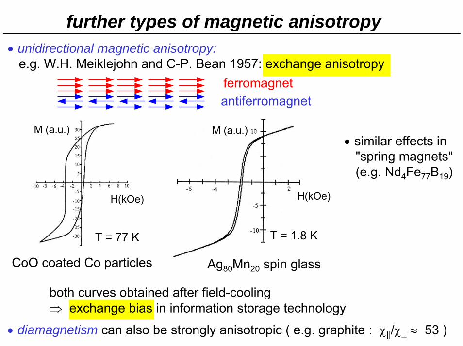
further types of magnetic anisotropy • unidirectional magnetic anisotropy:

e.g. W.H. Meiklejohn and C-P. Bean 1957: exchange anisotropy

• diamagnetism can also be strongly anisotropic ( e.g. graphite : χ||/χ⊥ ≈ 53 )

ferromagnetantiferromagnet

CoO coated Co particles

H(kOe)

M (a.u.) M (a.u.)

H(kOe)

T = 77 K T = 1.8 K

Ag80Mn20 spin glass

both curves obtained after field-cooling⇒ exchange bias in information storage technology

• similar effects in"spring magnets"(e.g. Nd4Fe77B19)

4-2 Magnetic anisotropy and coercivity• minimization of the free energy

∫ µ−µ

−−∇

τ=V

')()( ]2M

KM

A[dF 00

2s

2

2s

2

MHMHnMM

simplest form of magnetic anisotropy in uniaxial materials

⇒ at H = 0 a first order phase transition : M changes from nMs to – nMs

Fϑ

π 0

0 ≤ H < HA HA < HH < – HA – HA < H < 0

ϑM

n, H

JHc ≥ HA = 2 K/(µ0M) ⇒ for – JHc < H < 0 the magnetized state is metastable

• W.F. Brown (1963): not at H = 0 but at H = – JHc with

• observed JHc << HA ⇒ "Brown's paradox " ⇒ ⇒⇒ explained by imperfections in the material⇒ supported by thermal fluctuations and quantum tunneling⇒ soft magnetic materials : JHc << Ms⇒ hard magnetic (or permanent magnet) materials : JHc ≥ Ms

⇒ need of well defined microstructure ⇒ materials sciences

-HA

-JHc

H

M

H = 0

High-quality Nd-Fe-B permanent magnetssintered

1.5

1.0

0.5

0-0.5-1.0-1.5M

agne

tizat

ion

[Tes

la]

µ0H [ T ]

(BH)max ≈ 430kJ/m3

• µ0JHc ≈ 1.1 T (µ0HA ≈ 9 T)

• Br ≈ 1.5 T µ0Ms ≈ 1.6 T

• coercivity is controlled by nucleation of reverse domains

melt spun

-2.0 -1.5 -1.0 -0.5 0.00.00.20.40.60.81.01.21.4

hot pressed

die upset

Pol

ariz

atio

n J

[ T

]

External field µ0H [ T ]-2.0 -1.5 -1.0 -0.5 0

1.4

1.0

0.6

0.2

Mag

netiz

atio

n[T

esla

]

µ0H [ T ]

Magnetic after effect (or viscosity)

Hysteresis loop Viscosity experimentM(t) =M(0) + S ln(1 +t/t0)

µ 0M

[ T

]

-2.0 0-1.0 2.01.0

-1.0

0

1.0

•

•

••

µ0H [ T ]0 1 2 3 4 5 6

-475

-470

-465

-460

-455

-450

-445

t0 = 60 sS/Js = - 5.3 10-3

*S/Ms = -5·10-3

t0 = 60 s

ln(1 + t/t0)

103

·M/M

sNd4Fe77B19

– a further consequence of metastability –

Remagnetization effects– a further consequence of metastability –

0 1 2 3 4 50

5

10

15

20

25

t0 = 88 sS/Js = 5 10-4

Nd4Fe

77B

19

104 ·M

/Ms

ln(1 + t/t0)

S/Ms = 5·10-4

t0 = 88 s

• viscosity of opposite sign

2

4

300 4003500

Temperature [K]

102 ·M

/Ms

• thermal remagnetization

4-3 Magnetism in low dimensional systems• examples: cuprates known from high-Tc superconductors

with Cu++ (S = ħ/2) magnetic moments

plane: d = 2 chains: d = 1 isolated clusters: d = 0

dimer: d = 0Cu

O

LaCuO4

O

Cu

Sr2CuO3 Li2CuO2

Cu F

• if the CEF and the S - L-interaction of such systems are neglectedthey will be described by

Hex(i,j)= – J si sj

⇒ they are magnetically isotropic⇒ nevertheless their behaviour is very different because thermal as well as

quantum fluctuations make cooperative phenomena very sensitive to d

Cs3CuF6

d groundstate

µstagg/µB TN/| J | Tmax/| J|in χ(T)

χ(T→0)t ≡ T/|J|

3 Néel AFM 0.85 0.93 – ≈ const.

2 Néel AFM 0.61 0 0.94 0.04·(1 + t )1 spin liquid 0 – 0.64 ~ (1 + 0.5·ln(7.7/t))

0dimer

S = 0singlet

0 – 0.62 ~ e-1/t/t(spin gap)

0<−= ∑ JJ ji ssHrrSpin 1/2 Heisenberg antiferromagnet on simple cubic lattices

χJ/

Ng2 µ

B2

T/⎮J⎮

1 2 300.04

Curie

0.06

0.08

0.10

d = 2d = 3T

χ

TN

Curie

d = 1 and d = 0χ

T/⎮J⎮0 0.5 1.0

chain

dimer

Dimensionality crossover

• planes coupled by J⊥ with J⊥ < 0, | J⊥ | << | J | (d = 2)(C.M. Soukoulis et. al. 1991)

)3ln(32J/JJ4Tk NB

⊥

π=

⇒ nevertheless at high temperatures it behaves as a d = 2 system

⇒ a maximum of χ at kBTmax ≈ 0.94 J.

example : La2CuO4: kBJ ≈ 1500 K , J⊥/J ≈ 10-5 , resulting TN ≈ 300 KTmax ≈ 1400 K

⇒

5 - Phase transitions and magnetization processes5-1 Types of magnetic order

• ferromagnetic ground state: in all systems with J > 0⇒ also in d = 0 clusters and other low-d- systems

22121dim /)( ,,,, +−−+ ψψ−ψψ=Ψ

• antiferromagnetic order can only exist in infinitely large systems of sufficientlylarge dimensionality, d ≥ 2 ⇒ rich variety of different afm structures

• advanced technologies are neededneutron scattering, x-ray magnetic scattering, Mössbauer spectroscopy, nuclear magnetic resonance (NMR) and muon spin relaxation (µSR)

- remember the dimer with H = –Js1s2 , J < 0 , s1 = s2 = 1/2 ⇒ no antiferromagnet but a singlet state ⇒ no magnetic moments at the sites 1 and 2

• non-magnetic ground states with a spin gap alsoin spin-ladder compounds e.g. in SrCu2O3

O

Cu

• for J <0 or mixed values J 0 ⇒ much more complicated<>

The mixed-valence perovskite La1-xCaxMnO3

Aalternatingfm planesx = 0

Bfm

x = 0.3

Calternatingfm chainsx = 0.5

G"simple" afm

x = 1

• spin density waves and spiral structures due to exchange between the local magnetic moments mediated by itinerant electrons (RKKY)

Types of magnetic ordering• weak ferromagnetism for sufficiently low lattice symmetry the DM-interaction

⇒ small net magnetization (as e.g. in α-Fe2O3, La2CuO4)

inversion center

⇒ the center of inversion is not between the sites the afm sublattices ⇒ WFM

α-Fe2O3

• DM-interaction can also give rise to helical magnetization structures (e.g. MnSi)

M1

M2d ≠ 0

• ferrimagnets: a net magnetization arises because the magnetic moments are antiparallel and different in size e.g.Fe3O4, GdCo5

Magnetic structures in HoNi2B2Cdetermined by elastic neutron scattering

antiferromagnetic commensurate :

incommensurate c-axis modulated :(spiral structure)q = 0.916c*

Additionallythere is an incommensuratea-axis modulated with q = 0.585a*

Ho

a a

≈ 105°

≈ 75°

≈ 60°

≈ 90°

c

45°

Magnetic structures• frustration : if interactions (e.g. with next and overnext neighbours)

are in competition⇒ the system can form more than two magnetic sublattices

• in particular geometrical frustration (in e.g. the d = 3 pyrochlore lattice or the cubic Laves phase structure or the d = 2 Kagomé lattice

• spin glass states: caused by frustration in the presence of disordered solid structures (as e.g. amorphous solids)⇒ thermodynamic or kinetic "glass" state ?⇒ no equilibrium net magnetization⇒ nevertheless strong hysteresis phenomena

⇒ no long range order

frustration in a tetrahedron (as in the pyrochlore structure)with afm coupled spins i (i =1 … 4):⇒ the afm alignment cannot be satisfied, at the same time,

for all spin pairs

S1

S4

S3

S2

5-2 Magnetic domains

• fixed boundary magnetic moment direction⇒ due to the non-linearity of the problem a domain wall will be formed⇒ wall width (Nd2Fe14B : 3 nm)⇒ wall energy per unit area

A/K~δAK~γ

• Y. Imry and S.K. Ma (1975):in random anisotropy systems domain like structures⇒ competition of exchange and random anisotropy ⇒ even without magnetostatic selfenergy

• magnetostatic selfenergy: Edip ~ VM2 reduced by spontaneous formation of domains

• critical single-domain size 2s0c MAKD µ/~ (Nd2Fe14B : 300 nm)

• interaction domains in fine-grained polycrystalline permanent magnets

∫µ

−−∇

τ=V

')()( ]2M

KM

A[dF 02s

2

2s

2

MHnMMδ

easy

axi

s domaindomain

localization

Interaction domains in fine-grained materialsHot-deformed melt-spun Nd-Fe-B : grain size ≈ 200 …300 nm ≤ Dc ≈ 400 nm

10 µm 10 µm

20 µm 20 µm

thermally demagnetized dc-field demagnetized– by Kerr micoscopy –

Classical and Interaction DomainsHot-deformed melt-spun Nd-Fe-B

thermally demagnetized dc-field demagnetized

10 µm

– by Kerr micoscopy –

-4 -2 0 2 4-1,5

-1,0

-0,5

0,0

0,5

1,0

1,5

pola

risat

ion

J (T

)

applied field µ0H (T)

100µm

VACODYM 722HR

High-quality sintered Nd-FeB magnet

Kerr microscopy

High-quality Sm2Co17 sintered magnet

-4 -2 0 2 4-1,5

-1,0

-0,5

0,0

0,5

1,0

1,5

pola

risat

ionJ

(T)

applied field µ0H (T)

100µm

VACOMAX 240HR

Kerr microscopy

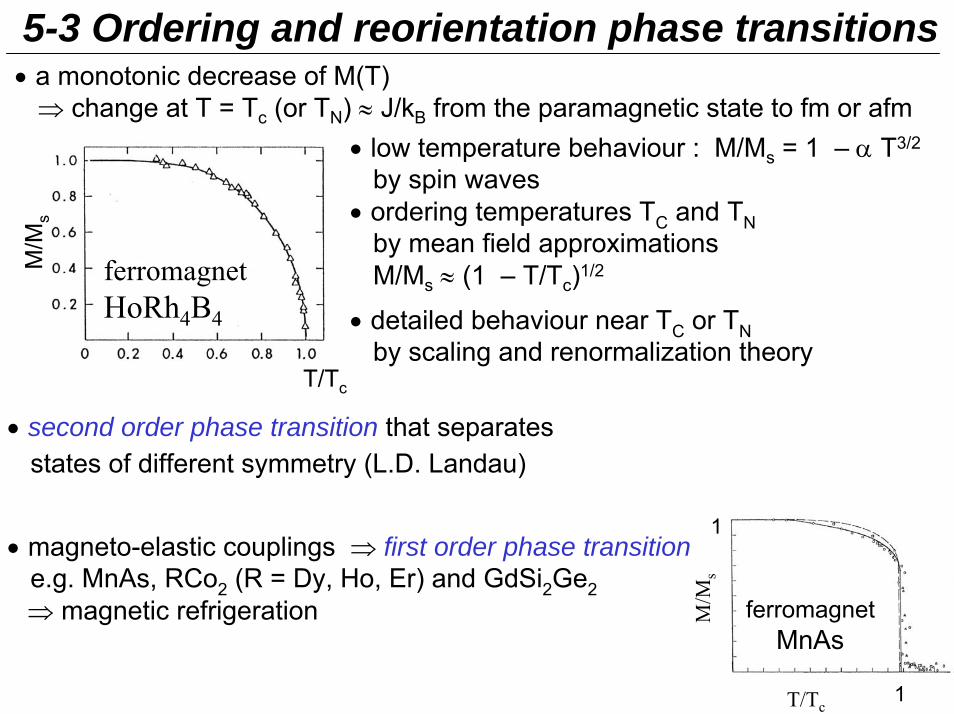
• a monotonic decrease of M(T)⇒ change at T = Tc (or TN) ≈ J/kB from the paramagnetic state to fm or afm

5-3 Ordering and reorientation phase transitions

• low temperature behaviour : M/Ms = 1 – α T3/2

by spin waves • ordering temperatures TC and TN

by mean field approximations M/Ms ≈ (1 – T/Tc)1/2

• detailed behaviour near TC or TNby scaling and renormalization theory

M/M

s

T/Tc

ferromagnetHoRh4B4

• second order phase transition that separates states of different symmetry (L.D. Landau)

M/M

sT/Tc

1

1

ferromagnetMnAs

• magneto-elastic couplings ⇒ first order phase transitione.g. MnAs, RCo2 (R = Dy, Ho, Er) and GdSi2Ge2 ⇒ magnetic refrigeration

Magnetic ordering• exact solution of the d=2 Ising model (L. Onsager 1944)

zj

ji,

zi ssJ∑−=H

M/M

s

K2CoF4

J < 0

T (K)

kB TN = 2.27J

M/Ms ≈ ( 1 – T/TN)1/8

⇒ strong influence of the dimensionality on the critical behaviour

(siz = ±1)

Magnetic ordering• if the strength of the coupling between subsystems is moderate

⇒ many different types of phase transitions

• e.g. : GdBa2Cu3O7- d = 2 sublattice of Cu++ magnetic moments order

antiferromagnetically at TN[Cu] ≈ 95 K - d ≈ 3 Gd-sublattice orders at TN[Gd] ≈ 2.2 K

• reentrant ferromagnetism in SmMn2Ge2

100 200 300Temperature (K)

15

10

5

SmMn2Ge2

Mag

netiz

atio

n (a

.u.)

Cu

O

Gd

a

c

Ba

Magnetic ordering• non-monotonic M(T) and compensation of different contributions

to M in ferrimagnets at T = Tcomp

• e.g. GdCo4B TC = 505 K and Tcomp = 410 K

M1 M2

ϑ

Ms

c

Magnetic ordering• spin reorientation transitions : contributions of different subsystems to magnetic anisotropy are different example Nd2Fe14B :

∫ +ϑ+ϑτ=V

][ K42

21A KKdE sinsin

i.e. K → K1 , …

K1 = K1[Nd] + K1[Fe] ⇒ ⇒ ⇒

⇒ a transition at T = TSR :easy axis → easy cone

K2K1

TSR = 135 K

tiltin

g an

gle

ϑt

TSR

temperature [ K ]

ϑt Msc

5-4 Metamagnetic transitions• field-induced magnetic phase transitions • spin-flip transition

if afm exchange is relatively weak compared to the anisotropy field• in DyCo2Si2 – A-type antiferromagnetic order with relatively weak

interaction between the fm planes

Dy

Co

Si

⇒

H (kOe)

DyCo2Si2H | | [001]

µ(µ

B/f.

u.)

Metamagnetic transitions• spin flop transition: If the exchange interaction in the antiferromagnet is

relatively strong compared to the anisotropy field

Ba3Cu2O4Cl2single crystal

T = 1.7K

H || cH || b

H || a

a-axis

H = 0⇐ •

⇐ Threshold field :

= 2K /(χ⊥ - χ||)Ht2

H > Ht⇐

T < TN ≈ 21K

Metamagnetic transitions• spin canting in ferrimagnets: a similar flopping phenomenon as the spin

flop transition, examples GdCo5, DyCo12B6

• second order phase transition ( spin flop is first order ! )- competition of exchange energy and field (Zeeman) energy

⇒

0 10 20 30 40 50 60

-10

-5

0

5

10

15

20

25

Hcr = 46 Tm

agne

tizat

ion

(arb

. uni

ts)

magnetic field (Tesla)

Co Gd

H H > Hcr

GdCo5

Gd

CoM

M1 M2

Hcr ∼ |J | | M1 – M2 |

T = 5 K

Metamagnetic transitions• First order magnetization processes (FOMPs):

⇒ competition of magnetostatic (Zeeman) energy with the anisotropy energy of different orders

-5 0 5 10 15 20 25

-20

-10

0

10

20

30

40Nd2Fe14B

H || a

mag

netis

atio

n [µ

B/f.

u.]

applied field µ0H [T]

130 K

30 K

FOMP

⇒ anisotropy in the tetragonal basal plane

Further forms of metamagnetic transitions• paramagnetic metamagnetism in cases of non-Kramers ions e.g. TmSb, PrNi5, Pr ⇒ from Van Vleck paramagnetism to Langevin-Curie paramagnetism

• itinerant electron metamagnetism (IEM): E.P. Wohlfarth and P. Rhodes (1962) ⇒ from Pauli paramagnetism to ferromagnetism, e.g. YCo2, LuCo2, La(Fe,Si)13

5-5 Quantum phase transitions • phase transitions at zero temperature (first or second order)• driven by quantum fluctuations instead of thermal fluctuations

⇒ modification of scaling and renormalization⇒ consequences of the quantum critical behaviour at non-zero temperature ?

∑∑ µ−−=i

xixB

ji,

zj

zi sHgssJH si

z = ± 1/2 , J > 0 ⇒ Ising ferromagnet

Temperature [ K ]

µ 0H

x [

T ]

0

6

4

2

• Ising ferromagnet LiHoF4in a field applied perpendicularly to its magnetic axisit becomes a (quantum) paramagnet

Quantum phase transitions• vanishing of the of the dimensionality crossover at a

quantum critical points (QCP)- e.g. two-leg ladders show a spin gap similar as dimers- if such ladders are coupled to each other by a small J⊥ the

crossover to 3d behaviour at low temperatures occurs onlyabove a critical value of J⊥/J

J' = JJ

J⊥⇒ ⇒

J⊥/J

T N /J

0.2 0.4 0.6 0.8 10

0.5

1.0

1.5

0

QCP

• on the other hand, if chains are coupled by J'the spin gap ∆ opens immediately upon the introduction of non-zero J'⇒ no QCP Barnes et al.

1993

0.5

0 1.0 2.0J'/J

∆/J

basics and magnetic materials - magnetism.eu - ema - the european magnetism...

Documents