basics of experimental design for fmri: event-related designs last update: january 18, 2012 last...
TRANSCRIPT

Basics of Experimental Designfor fMRI:
Event-Related Designs
http://www.fmri4newbies.com/
Last Update: January 18, 2012Last Course: Psychology 9223, W2010, University of Western Ontario
Jody CulhamBrain and Mind Institute
Department of PsychologyUniversity of Western Ontario
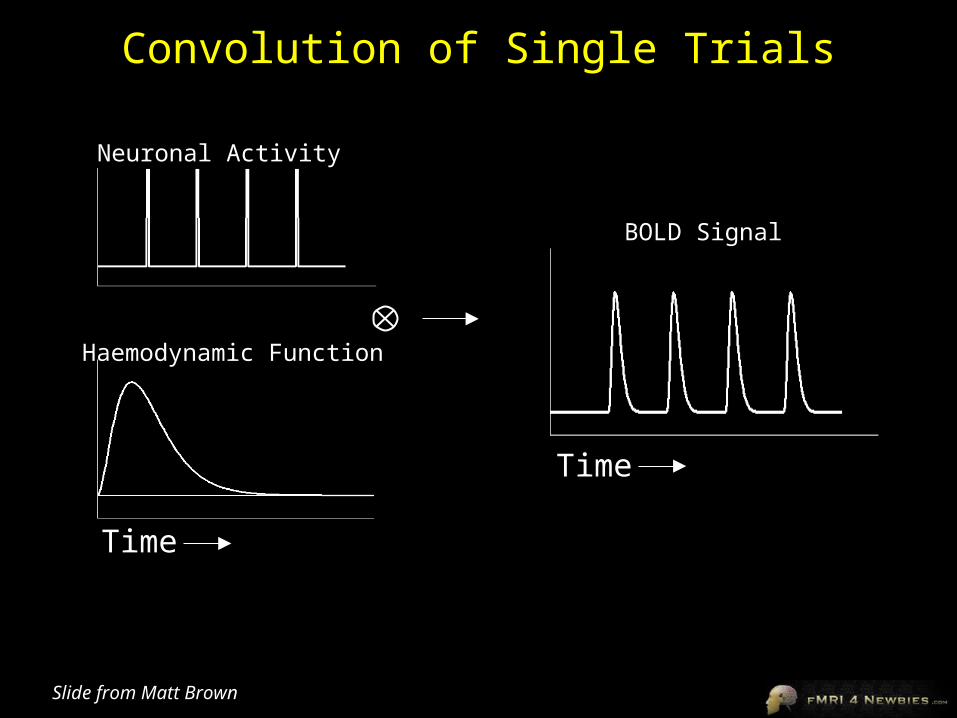
Convolution of Single Trials
Neuronal Activity
Haemodynamic Function
BOLD Signal
Time
Time
Slide from Matt Brown
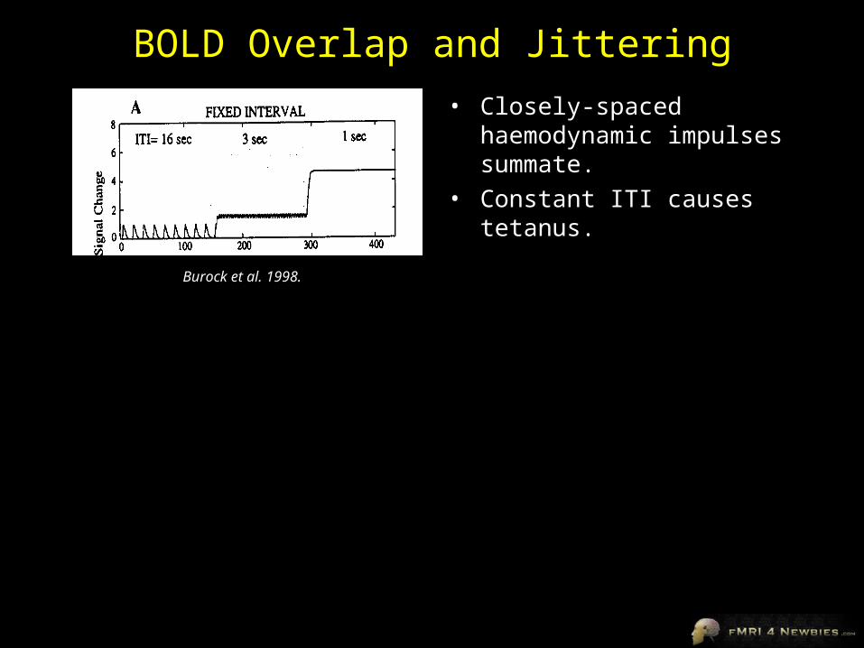
BOLD Overlap and Jittering
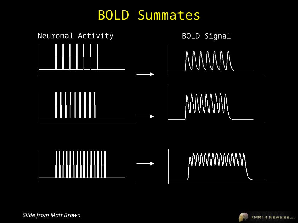
• Closely-spaced haemodynamic impulses summate.
• Constant ITI causes tetanus.
Burock et al. 1998.
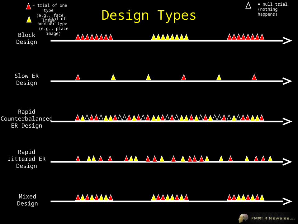
Design TypesBlock
Design
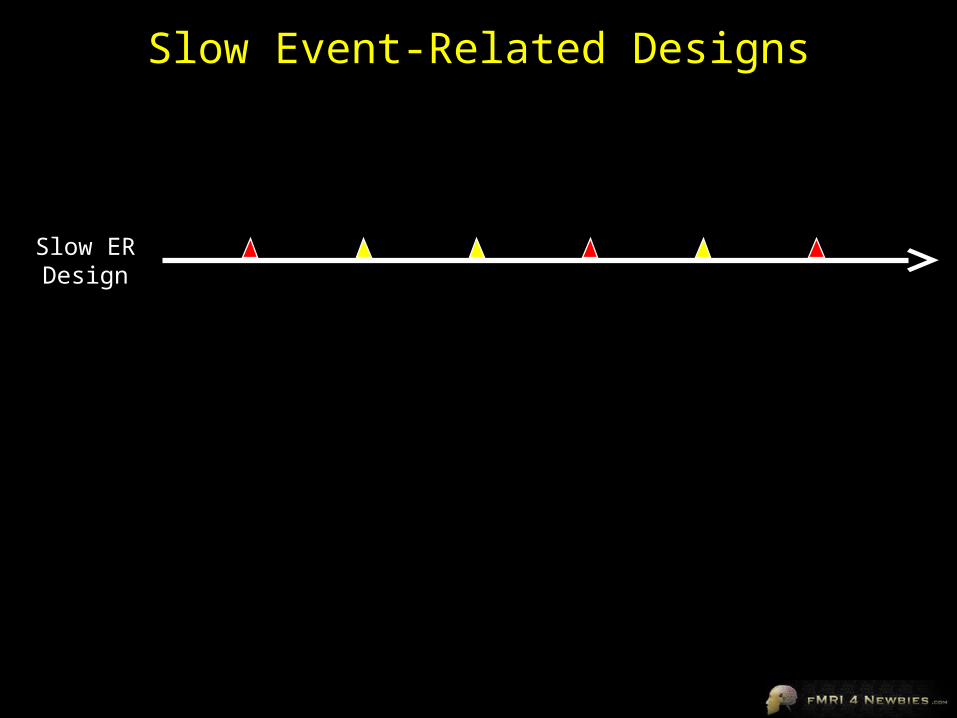
Slow ERDesign
RapidCounterbalanced
ER Design
RapidJittered ER
Design
MixedDesign
= null trial (nothing happens)
= trial of one type (e.g., face image)
= trial of another type (e.g., place image)
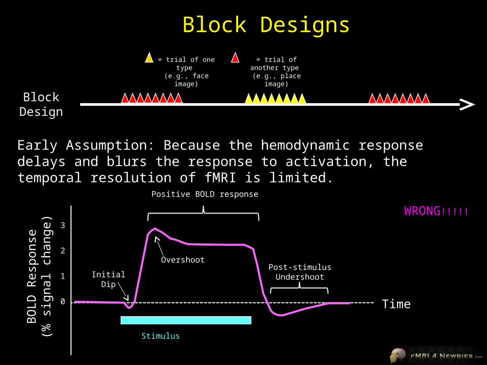
Block Designs
Early Assumption: Because the hemodynamic response delays and blurs the response to activation, the temporal resolution of fMRI is limited.
= trial of one type (e.g., face image)
= trial of another type (e.g., place image)
WRONG!!!!!
BlockDesign
Positive BOLD response
InitialDip
OvershootPost-stimulusUndershoot
0
1
2
3
BO
LD R
espo
nse
(% s
igna
l cha
nge)
Time
Stimulus
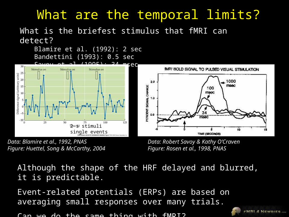
What are the temporal limits?What is the briefest stimulus that fMRI can detect?
Blamire et al. (1992): 2 secBandettini (1993): 0.5 secSavoy et al (1995): 34 msec
Although the shape of the HRF delayed and blurred, it is predictable.
Event-related potentials (ERPs) are based on averaging small responses over many trials.
Can we do the same thing with fMRI?
Data: Blamire et al., 1992, PNASFigure: Huettel, Song & McCarthy, 2004
2 s stimulisingle events
Data: Robert Savoy & Kathy O’CravenFigure: Rosen et al., 1998, PNAS
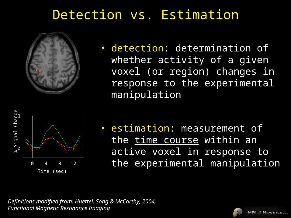
Detection vs. Estimation
• detection: determination of whether activity of a given voxel (or region) changes in response to the experimental manipulation
Definitions modified from: Huettel, Song & McCarthy, 2004, Functional Magnetic Resonance Imaging
% S
ign
al C
ha
ng
e
0
Time (sec)
0 4 8 12
1
• estimation: measurement of the time course within an active voxel in response to the experimental manipulation
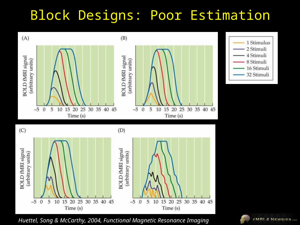
Block Designs: Poor Estimation
Huettel, Song & McCarthy, 2004, Functional Magnetic Resonance Imaging
Pros & Cons of Block Designs
Pros• high detection power• has been the most widely used approach for fMRI studies• accurate estimation of hemodynamic response function is not
as critical as with event-related designs
Cons• poor estimation power• subjects get into a mental set for a block• very predictable for subject• can’t look at effects of single events (e.g., correct vs. incorrect
trials, remembered vs. forgotten items)• becomes unmanagable with too many conditions (e.g., more
than 4 conditions + baseline)
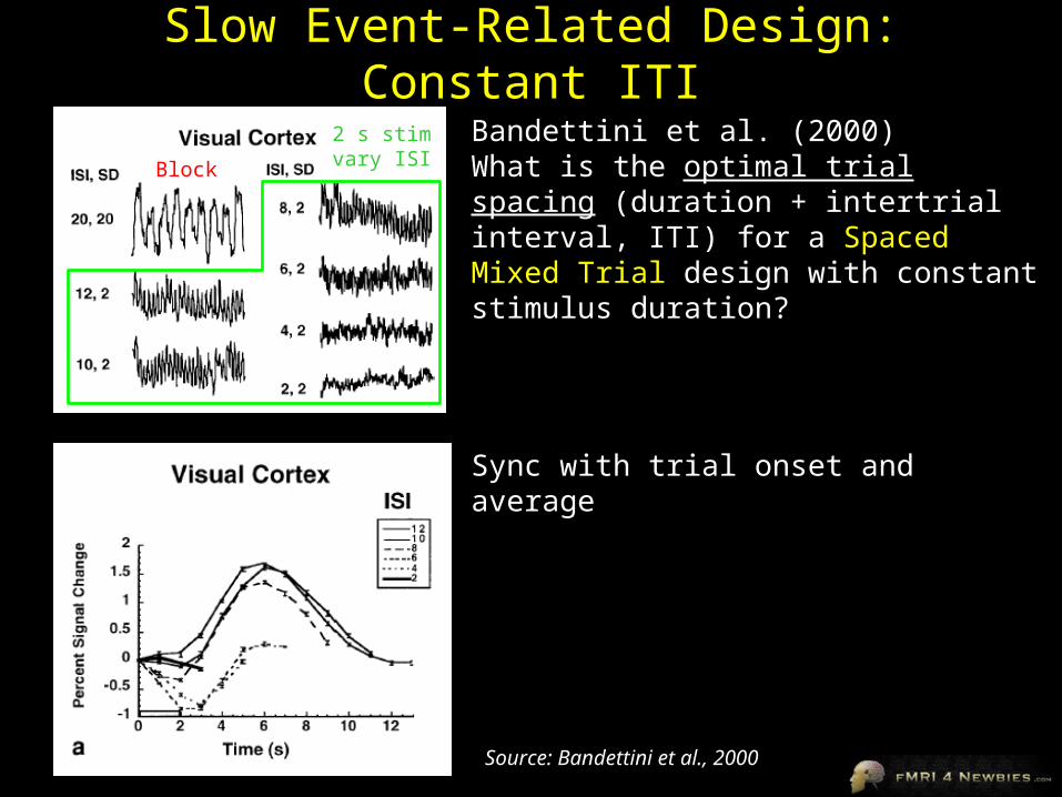
Slow Event-Related Design: Constant ITI
Bandettini et al. (2000)What is the optimal trial spacing (duration + intertrial interval, ITI) for a Spaced Mixed Trial design with constant stimulus duration?
Block
2 s stimvary ISI
Sync with trial onset and average
Source: Bandettini et al., 2000
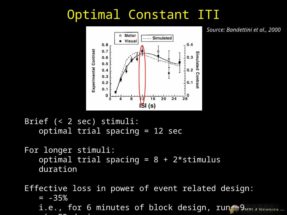
Optimal Constant ITI
Brief (< 2 sec) stimuli:optimal trial spacing = 12 sec
For longer stimuli:optimal trial spacing = 8 + 2*stimulus duration
Effective loss in power of event related design:= -35%i.e., for 6 minutes of block design, run ~9 min ER design
Source: Bandettini et al., 2000
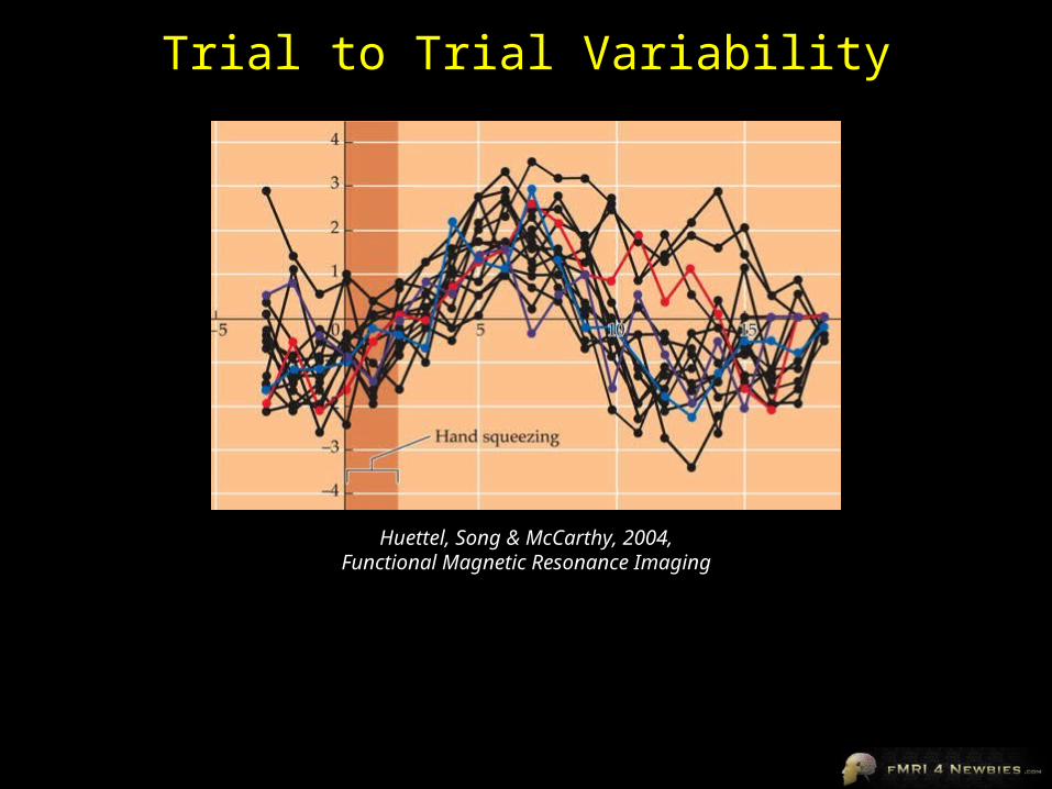
Trial to Trial Variability
Huettel, Song & McCarthy, 2004,Functional Magnetic Resonance Imaging
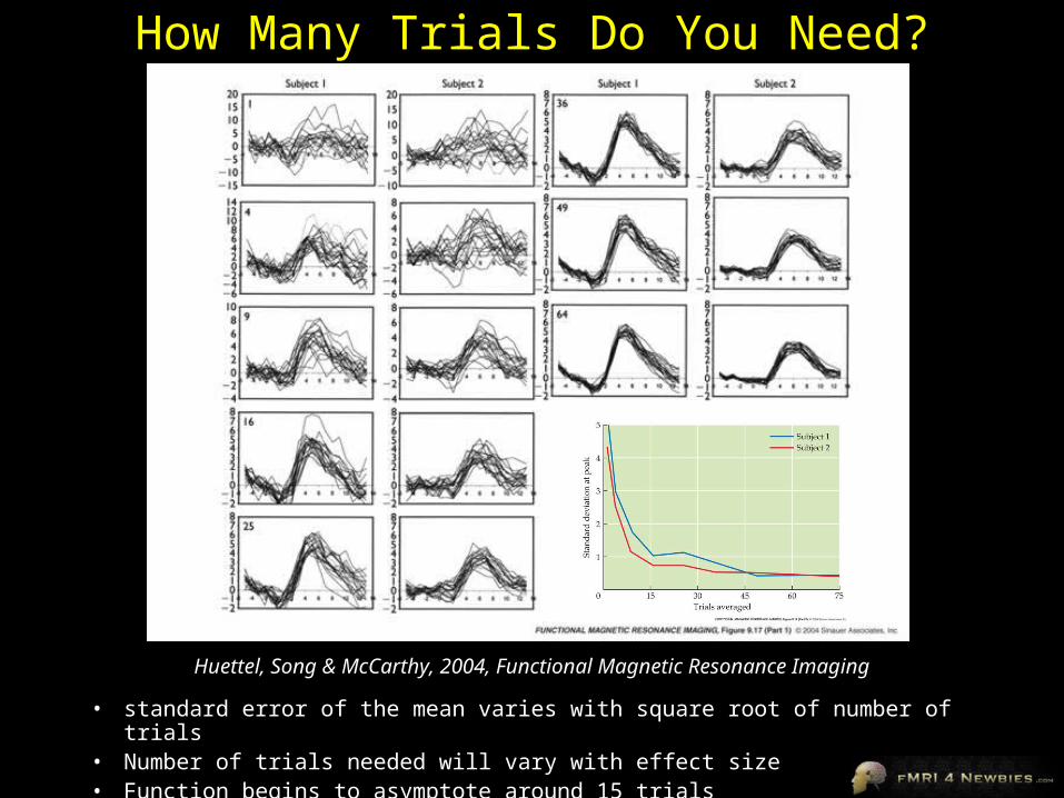
How Many Trials Do You Need?
• standard error of the mean varies with square root of number of trials• Number of trials needed will vary with effect size• Function begins to asymptote around 15 trials
Huettel, Song & McCarthy, 2004, Functional Magnetic Resonance Imaging
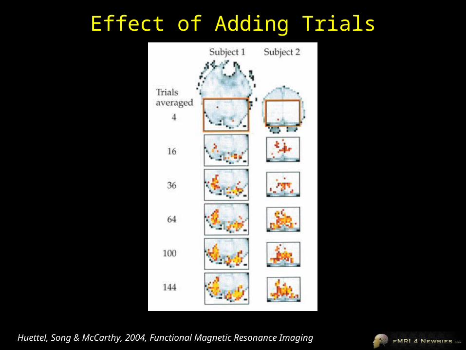
Effect of Adding Trials
Huettel, Song & McCarthy, 2004, Functional Magnetic Resonance Imaging
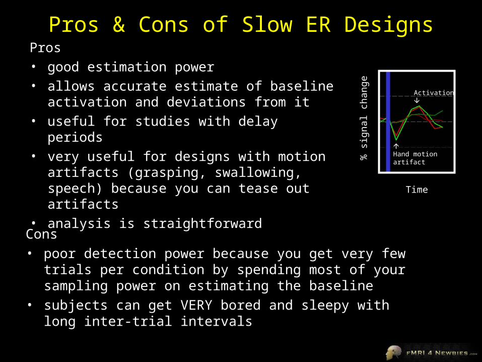
Pros & Cons of Slow ER DesignsPros• good estimation power• allows accurate estimate of baseline activation
and deviations from it• useful for studies with delay periods• very useful for designs with motion artifacts
(grasping, swallowing, speech) because you can tease out artifacts
• analysis is straightforward
Cons• poor detection power because you get very few trials per
condition by spending most of your sampling power on estimating the baseline
• subjects can get VERY bored and sleepy with long inter-trial intervals
Hand motionartifact
% s
igna
l cha
nge
Time
Activation
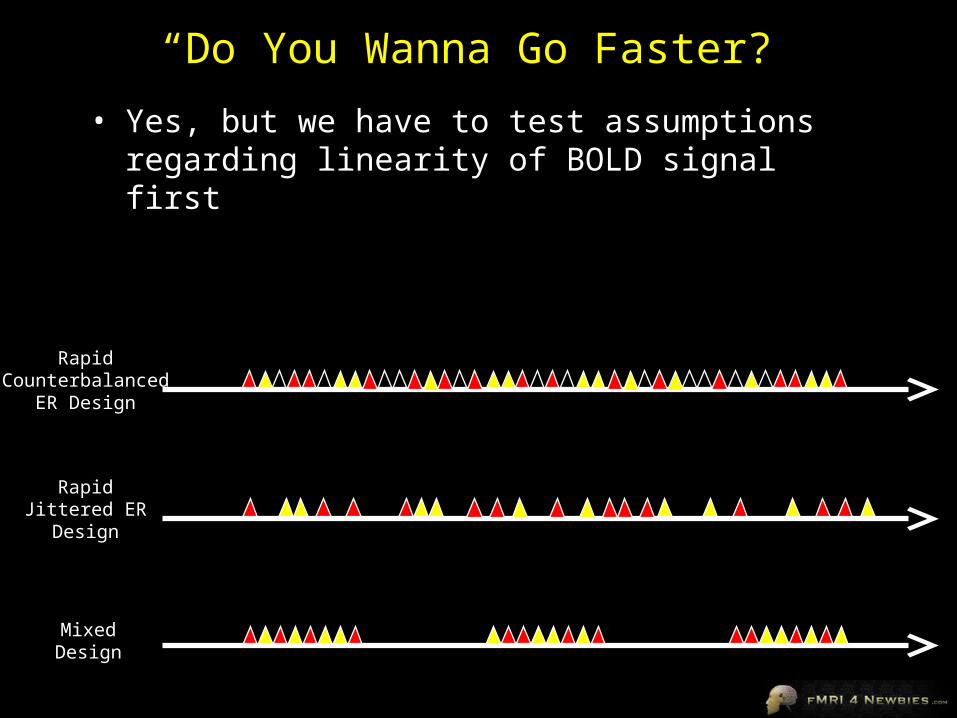
“Do You Wanna Go Faster?”
• Yes, but we have to test assumptions regarding linearity of BOLD signal first
RapidJittered ER
Design
MixedDesign
RapidCounterbalanced
ER Design
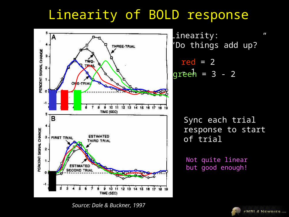
Linearity of BOLD response
Source: Dale & Buckner, 1997
Linearity:“Do things add up?”
red = 2 - 1
green = 3 - 2
Sync each trial response to start of trial
Not quite linear but good enough!
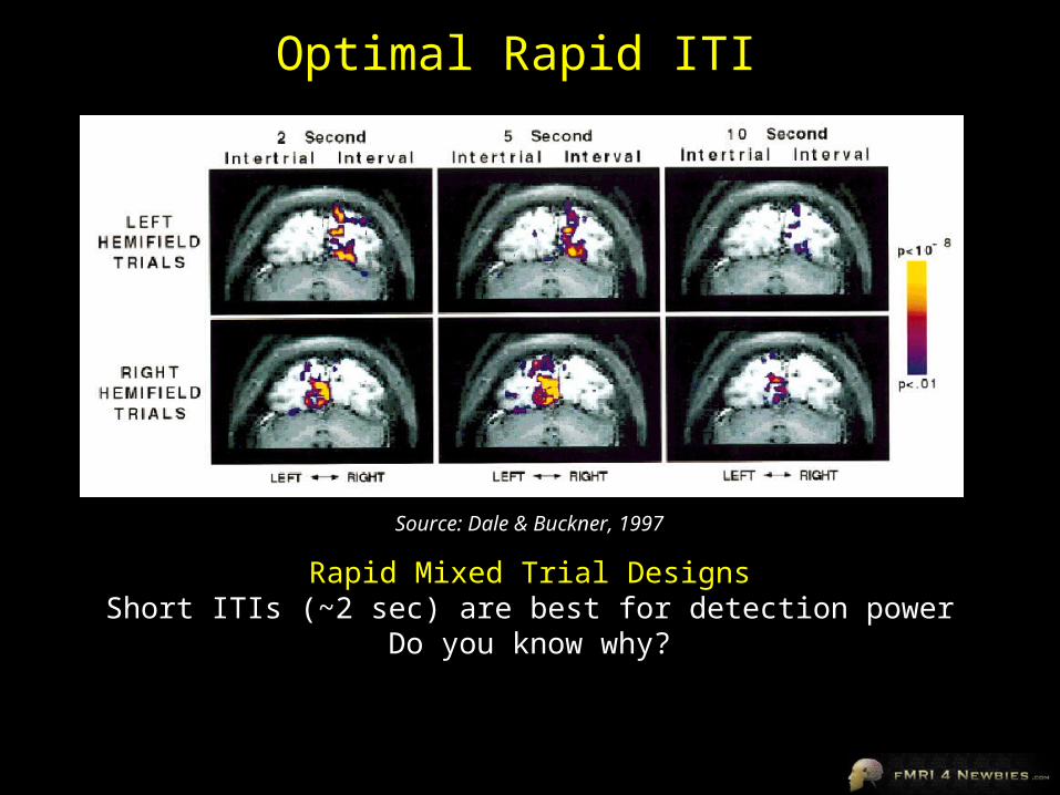
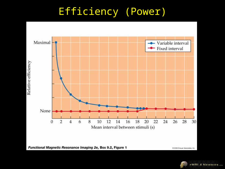
Optimal Rapid ITI
Rapid Mixed Trial DesignsShort ITIs (~2 sec) are best for detection power
Do you know why?
Source: Dale & Buckner, 1997
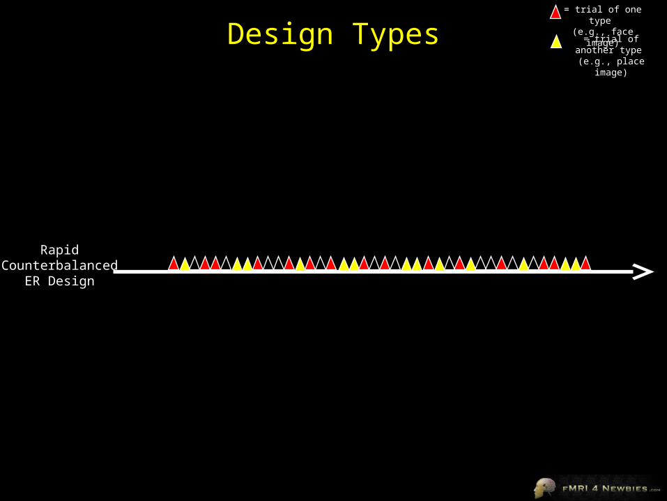
Design Types= trial of one type (e.g., face image)
= trial of another type (e.g., place image)
RapidCounterbalanced
ER Design
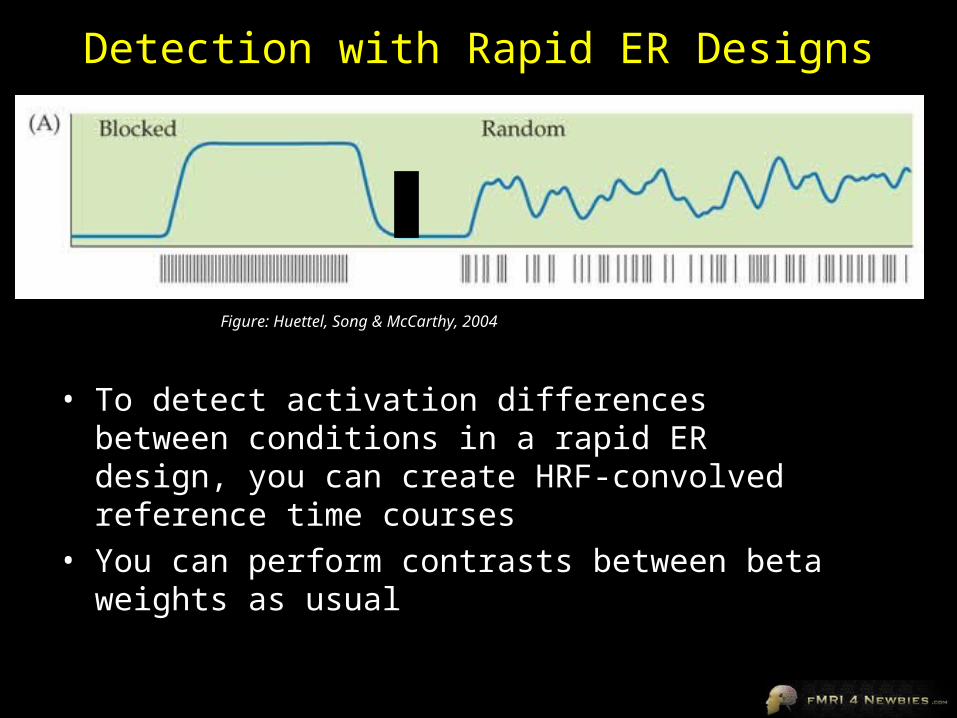
Detection with Rapid ER Designs
• To detect activation differences between conditions in a rapid ER design, you can create HRF-convolved reference time courses
• You can perform contrasts between beta weights as usual
Figure: Huettel, Song & McCarthy, 2004
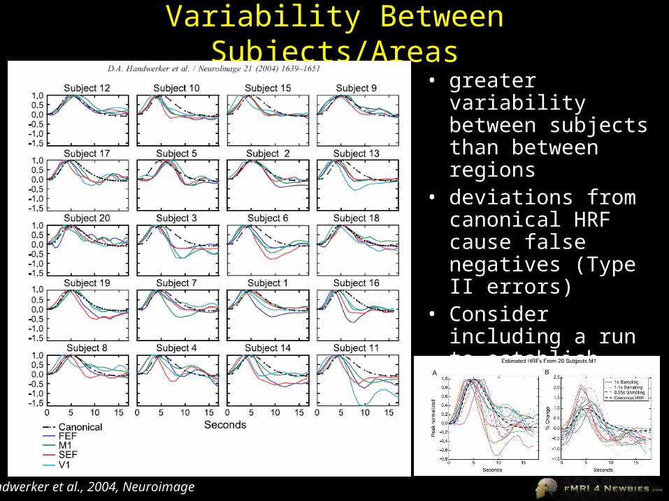
Variability Between Subjects/Areas
• greater variability between subjects than between regions
• deviations from canonical HRF cause false negatives (Type II errors)
• Consider including a run to establish subject-specific HRFs from robust area like M1
Handwerker et al., 2004, Neuroimage
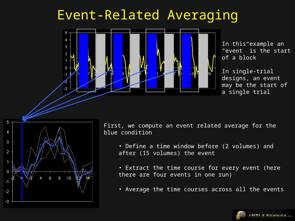
Event-Related Averaging
In this example an “event” is the start of a block
In single-trial designs, an event may be the start of a single trial
First, we compute an event related average for the blue condition
• Define a time window before (2 volumes) and after (15 volumes) the event
• Extract the time course for every event (here there are four events in one run)
• Average the time courses across all the events
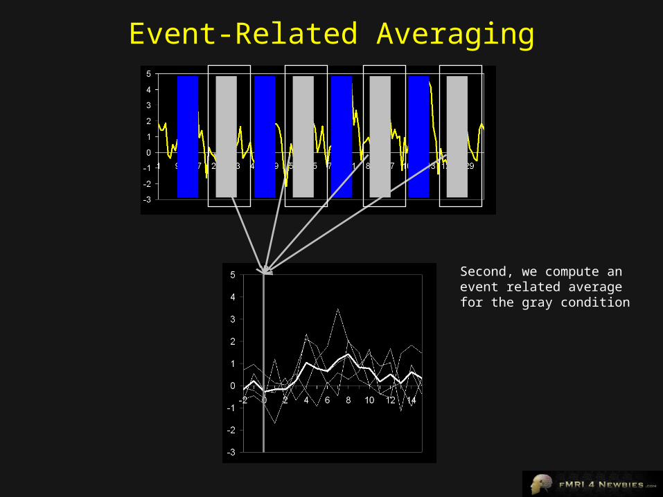
Event-Related Averaging
Second, we compute an event related average for the gray condition
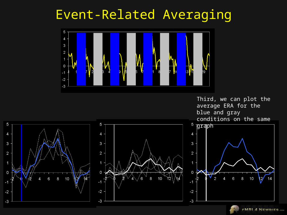
Event-Related Averaging
Third, we can plot the average ERA for the blue and gray conditions on the same graph
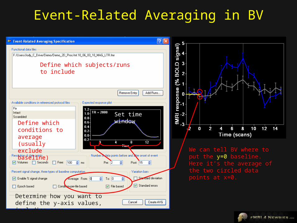
Event-Related Averaging in BV
Define which subjects/runs to include
Define which conditions to average (usually exclude baseline)
Set time window
Determine how you want to define the y-axis values, including zero
We can tell BV where to put the y=0 baseline. Here it’s the average of the two circled data points at x=0.
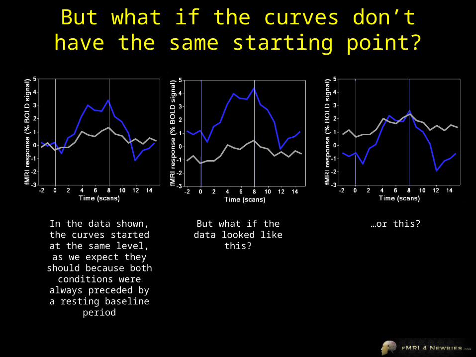
But what if the curves don’t have the same starting point?
In the data shown, the curves started at the same
level, as we expect they should because both
conditions were always preceded by a resting
baseline period
But what if the data looked like this?
…or this?
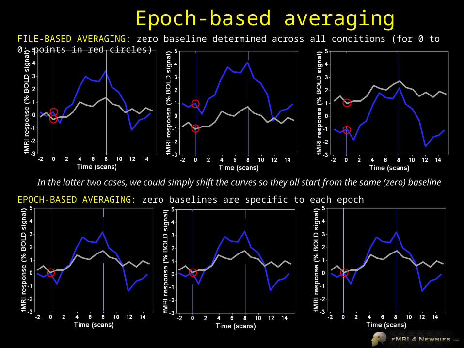
Epoch-based averaging
In the latter two cases, we could simply shift the curves so they all start from the same (zero) baseline
FILE-BASED AVERAGING: zero baseline determined across all conditions (for 0 to 0: points in red circles)
EPOCH-BASED AVERAGING: zero baselines are specific to each epoch
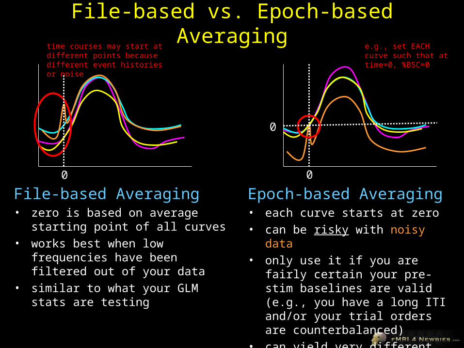
File-based vs. Epoch-based Averaging
File-based Averaging• zero is based on average starting point
of all curves
• works best when low frequencies have been filtered out of your data
• similar to what your GLM stats are testing
time courses may start at different points because different event histories or noise
0
Epoch-based Averaging• each curve starts at zero
• can be risky with noisy data
• only use it if you are fairly certain your pre-stim baselines are valid (e.g., you have a long ITI and/or your trial orders are counterbalanced)
• can yield very different conclusions than GLM stats
e.g., set EACH curve such that at time=0, %BSC=0
0
0
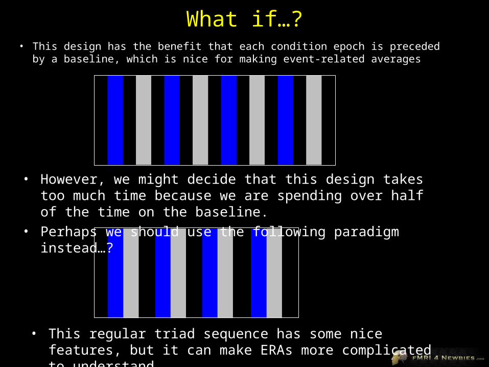
What if…?• This design has the benefit that each condition epoch is preceded
by a baseline, which is nice for making event-related averages
• However, we might decide that this design takes too much time because we are spending over half of the time on the baseline.
• Perhaps we should use the following paradigm instead…?
• This regular triad sequence has some nice features, but it can make ERAs more complicated to understand.
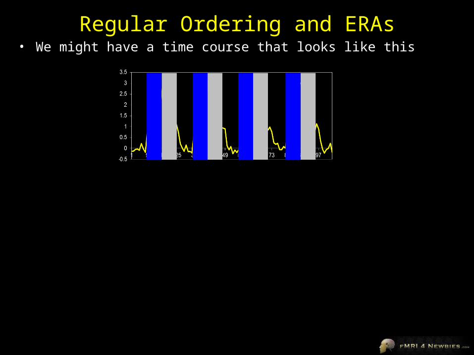
Regular Ordering and ERAs• We might have a time course that looks like this
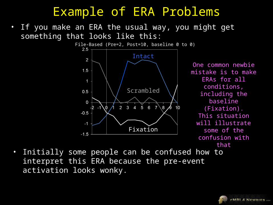
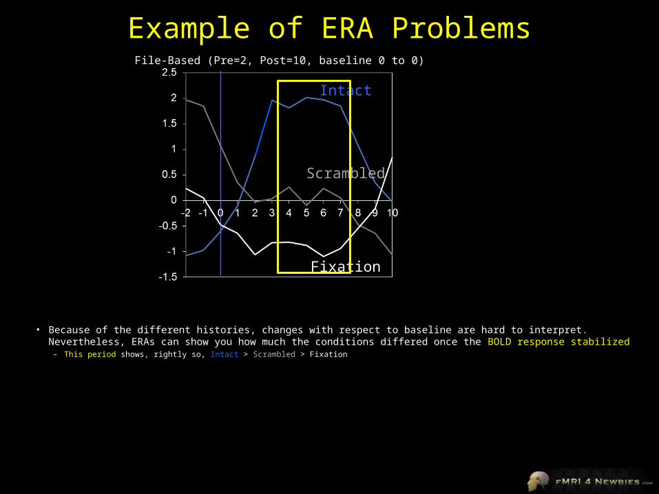
Example of ERA Problems• If you make an ERA the usual way, you might get something that
looks like this:
• Initially some people can be confused how to interpret this ERA because the pre-event activation looks wonky.
Intact
Scrambled
Fixation
One common newbie mistake is to make
ERAs for all conditions, including
the baseline (Fixation).
This situation will illustrate some of the confusion with that
File-Based (Pre=2, Post=10, baseline 0 to 0)
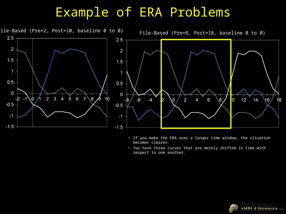
Example of ERA Problems
• If you make the ERA over a longer time window, the situation becomes clearer. • You have three curves that are merely shifted in time with respect to one
another.
File-Based (Pre=2, Post=10, baseline 0 to 0) File-Based (Pre=8, Post=18, baseline 0 to 0)
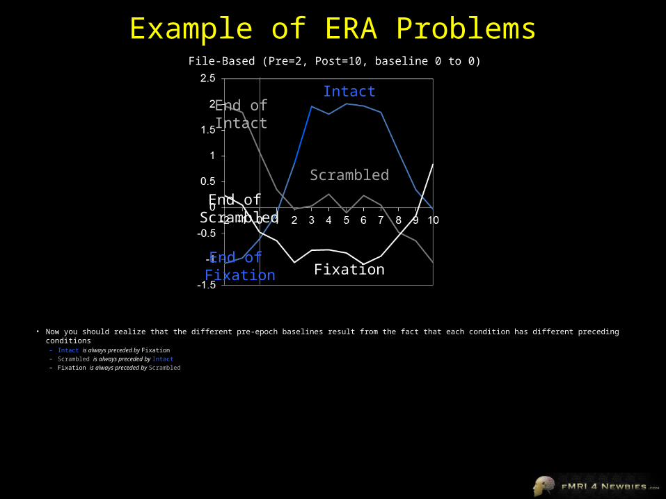
Example of ERA Problems
• Now you should realize that the different pre-epoch baselines result from the fact that each condition has different preceding conditions– Intact is always preceded by Fixation– Scrambled is always preceded by Intact– Fixation is always preceded by Scrambled
Intact
Scrambled
Fixation
End ofIntact
End of Scrambled
End of Fixation
File-Based (Pre=2, Post=10, baseline 0 to 0)
Example of ERA Problems
• Because of the different histories, changes with respect to baseline are hard to interpret. Nevertheless, ERAs can show you how much the conditions differed once the BOLD response stabilized
– This period shows, rightly so, Intact > Scrambled > Fixation
Intact
Scrambled
Fixation
File-Based (Pre=2, Post=10, baseline 0 to 0)
Example of ERA Problems
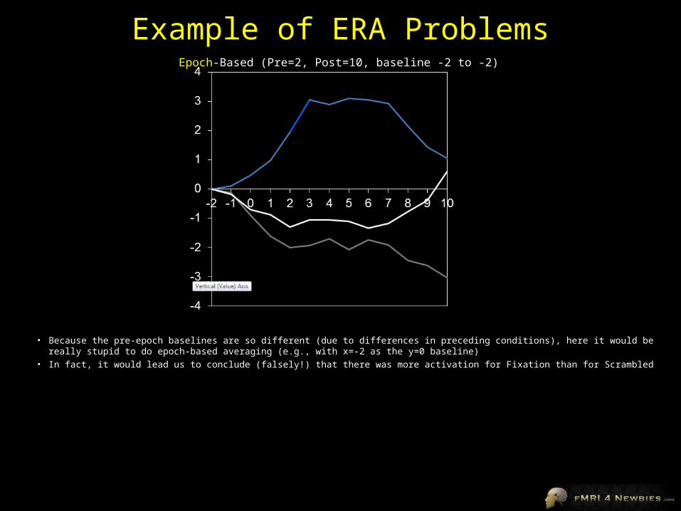
• Because the pre-epoch baselines are so different (due to differences in preceding conditions), here it would be really stupid to do epoch-based averaging (e.g., with x=-2 as the y=0 baseline)
• In fact, it would lead us to conclude (falsely!) that there was more activation for Fixation than for Scrambled
Epoch-Based (Pre=2, Post=10, baseline -2 to -2)
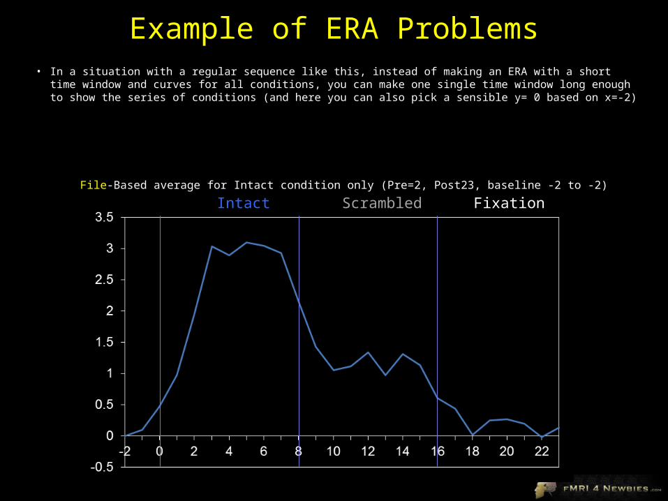
Example of ERA Problems• In a situation with a regular sequence like this, instead of making an ERA with a short time window and
curves for all conditions, you can make one single time window long enough to show the series of conditions (and here you can also pick a sensible y= 0 based on x=-2)
Intact Scrambled FixationFile-Based average for Intact condition only (Pre=2, Post23, baseline -2 to -2)
Partial confounding
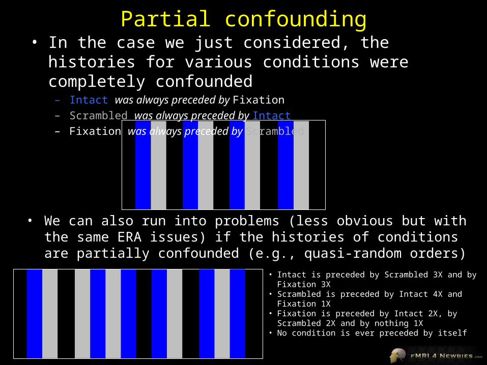
• We can also run into problems (less obvious but with the same ERA issues) if the histories of conditions are partially confounded (e.g., quasi-random orders)
• In the case we just considered, the histories for various conditions were completely confounded
– Intact was always preceded by Fixation– Scrambled was always preceded by Intact– Fixation was always preceded by Scrambled
• Intact is preceded by Scrambled 3X and by Fixation 3X• Scrambled is preceded by Intact 4X and Fixation 1X• Fixation is preceded by Intact 2X, by Scrambled 2X and
by nothing 1X• No condition is ever preceded by itself
The Problem of Trial/Block History
This problem also occurs for single trial designs.
This problem also occurs even if the history is only partially confounded (e.g., if Condition A is preceded by Condition X twice as often as Condition B is preceded by Condition X).
If we knew with certainty what a given subject’s HRF looked like, we could model it (but that’s rarely the case).
Thus we have only two solutions: 1) Counterbalance trial history so that each curve should start with the
same baseline2) Jitter the intertrial intervals so that we can estimate the HRF
• more on this in analysis when we talk about deconvolution
One Approach to Estimation: Counterbalanced Trial Orders
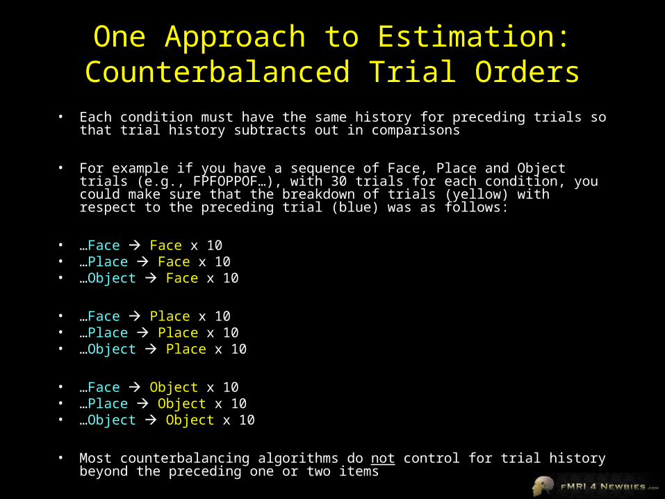
• Each condition must have the same history for preceding trials so that trial history subtracts out in comparisons
• For example if you have a sequence of Face, Place and Object trials (e.g., FPFOPPOF…), with 30 trials for each condition, you could make sure that the breakdown of trials (yellow) with respect to the preceding trial (blue) was as follows:
• …Face Face x 10• …Place Face x 10• …Object Face x 10
• …Face Place x 10• …Place Place x 10• …Object Place x 10
• …Face Object x 10• …Place Object x 10• …Object Object x 10
• Most counterbalancing algorithms do not control for trial history beyond the preceding one or two items
Analysis of Single Trials with Counterbalanced Orders
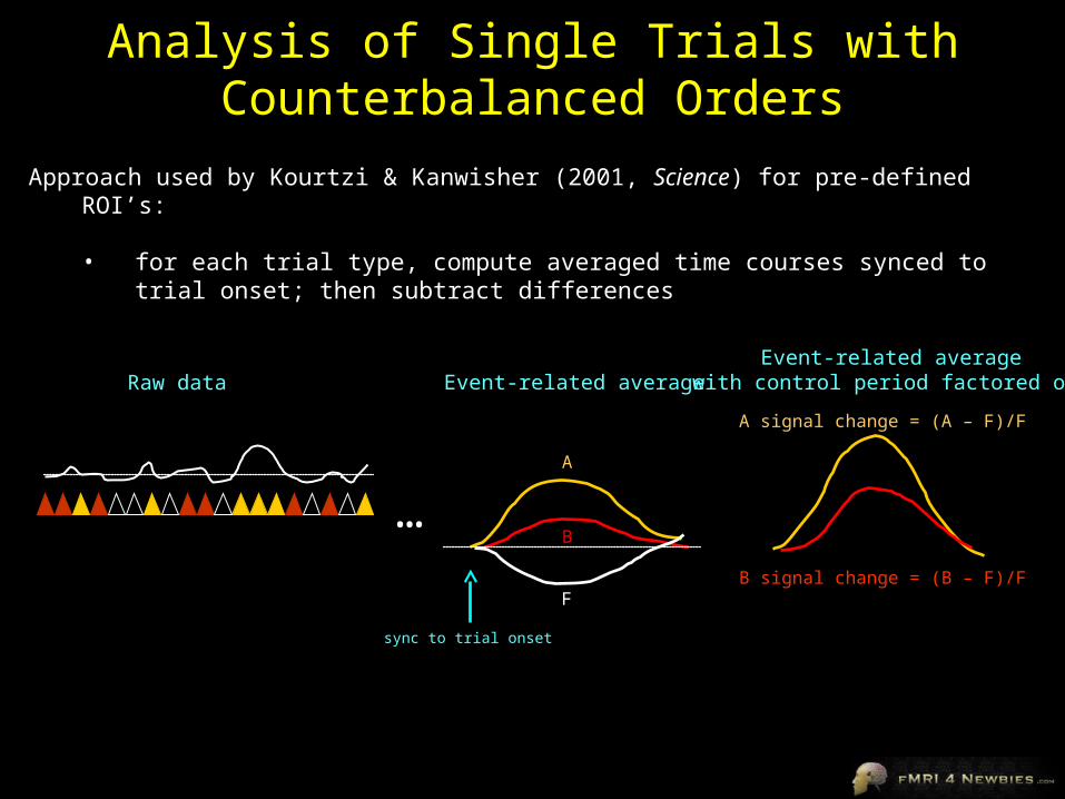
Approach used by Kourtzi & Kanwisher (2001, Science) for pre-defined ROI’s:
• for each trial type, compute averaged time courses synced to trial onset; then subtract differences
…
Raw dataEvent-related average
with control period factored out
A signal change = (A – F)/F
B signal change = (B – F)/F
Event-related average
sync to trial onset
A
B
F
Pros & Cons of Counterbalanced Rapid ER Designs
Pros
• high detection power with advantages of ER designs (e.g., can have many trial types in an unpredictable order)
Cons and Caveats
• reduced detection compared to block designs
• estimation power is better than block designs but not great
• accurate detection requires accurate HRF modelling
• counterbalancing only considers one or two trials preceding each stimulus; have to assume that higher-order history is random enough not to matter
• what do you do with the trials at the beginning of the run… just throw them out?
• you can’t exclude error trials and keep counterbalanced trial history
• you can’t use this approach when you can’t control trial status (e.g., items that are later remembered vs. forgotten)
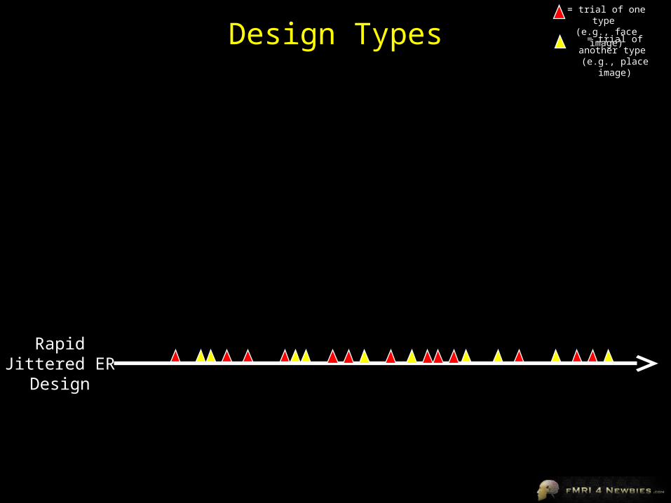
Design Types
RapidJittered ER
Design
= trial of one type (e.g., face image)
= trial of another type (e.g., place image)
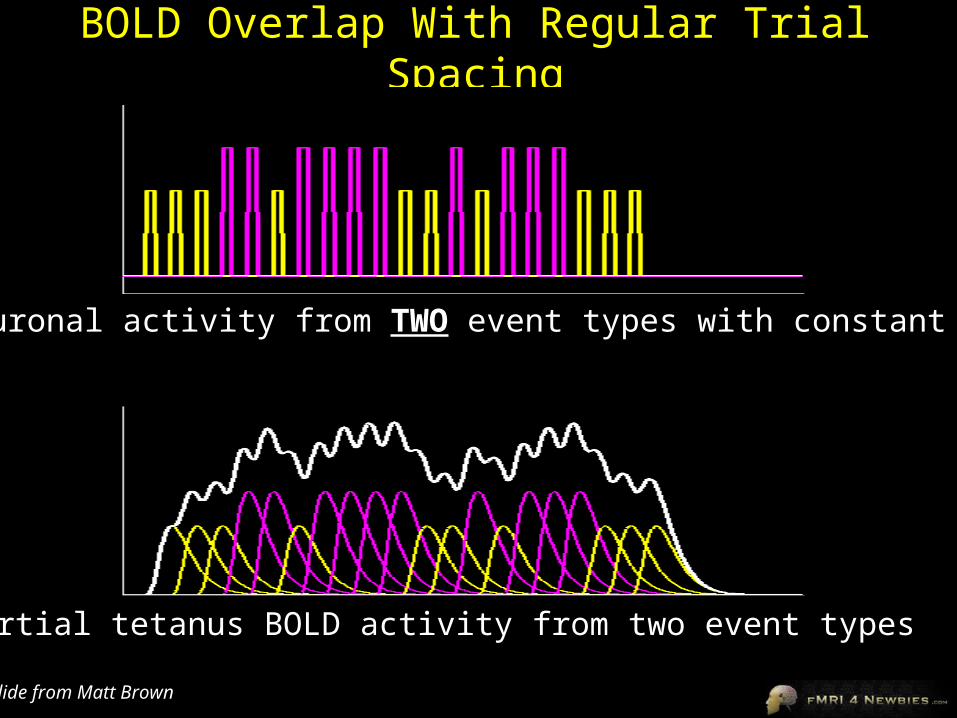
BOLD Overlap With Regular Trial Spacing
Neuronal activity from TWO event types with constant ITI
Partial tetanus BOLD activity from two event types
Slide from Matt Brown
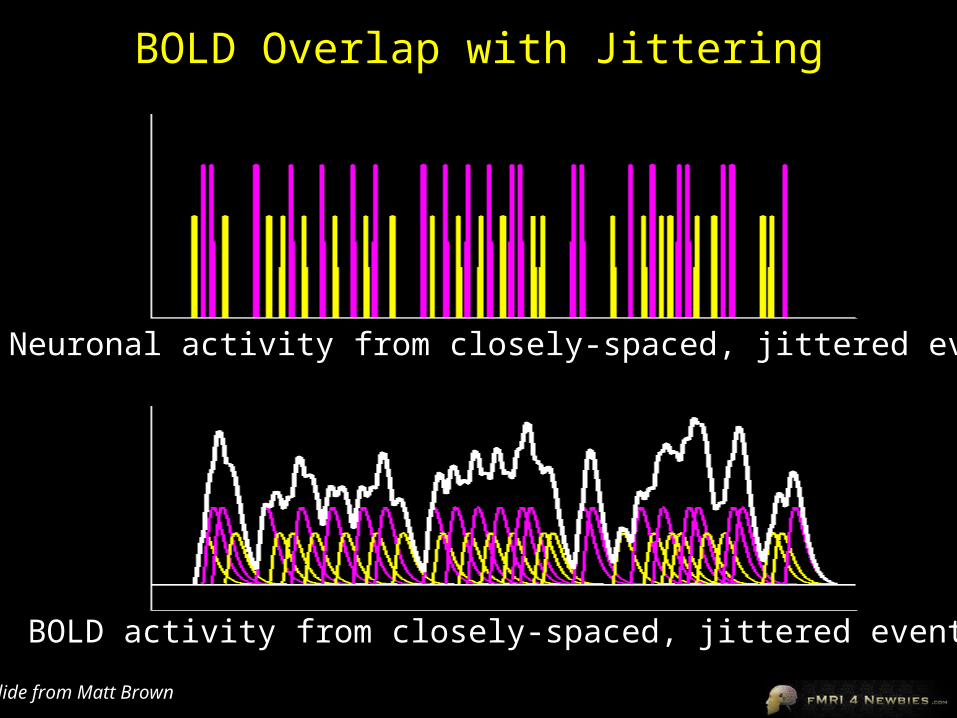
BOLD Overlap with Jittering
Neuronal activity from closely-spaced, jittered events
BOLD activity from closely-spaced, jittered events
Slide from Matt Brown

BOLD Overlap with Jittering
Neuronal activity from closely-spaced, jittered events
BOLD activity from closely-spaced, jittered events
Slide from Matt Brown
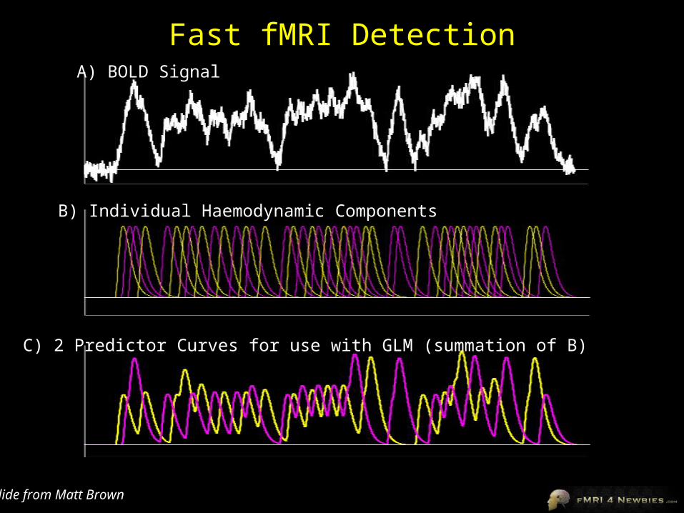
Fast fMRI DetectionA) BOLD Signal
B) Individual Haemodynamic Components
C) 2 Predictor Curves for use with GLM (summation of B)
Slide from Matt Brown

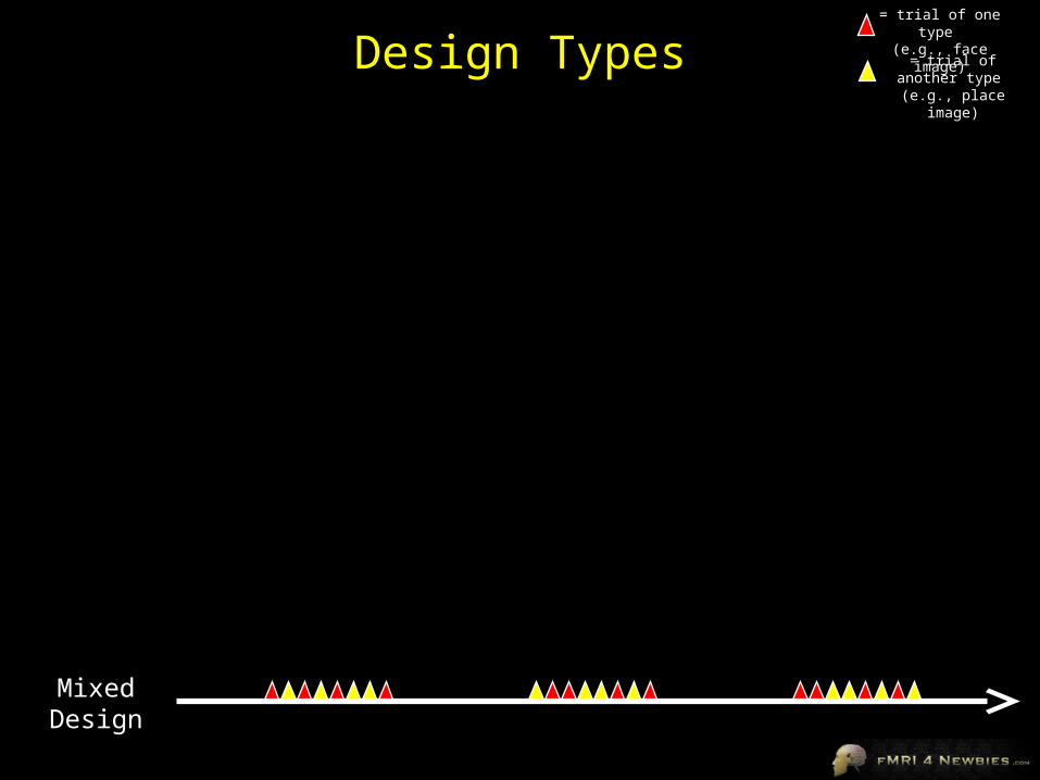
Design Types
MixedDesign
= trial of one type (e.g., face image)
= trial of another type (e.g., place image)
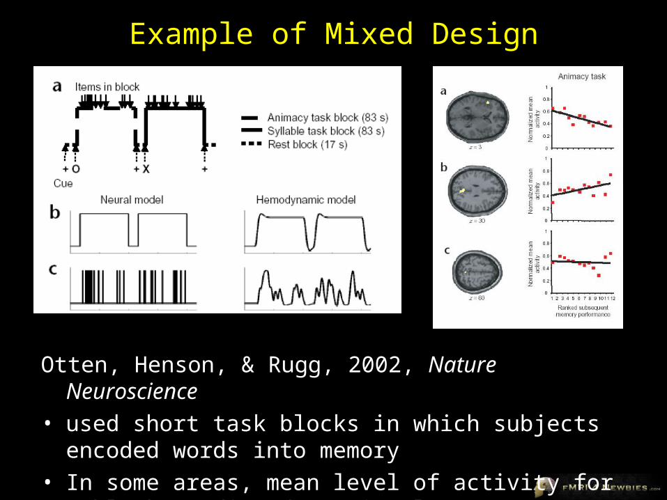
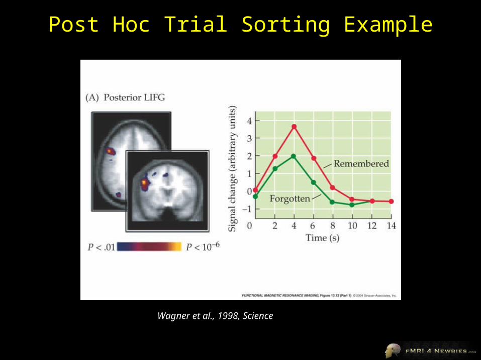
Example of Mixed Design
Otten, Henson, & Rugg, 2002, Nature Neuroscience• used short task blocks in which subjects encoded words
into memory • In some areas, mean level of activity for a block
predicted retrieval success
Pros and Cons of Mixed Designs
Pros• allow researchers to distinguish between state-
related and item-related activation
Cons• sensitive to errors in HRF modelling

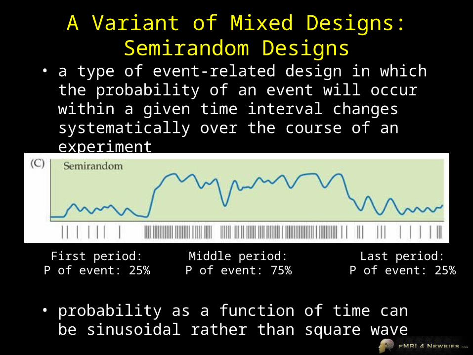
A Variant of Mixed Designs: Semirandom Designs
• a type of event-related design in which the probability of an event will occur within a given time interval changes systematically over the course of an experiment
First period:P of event: 25%
Middle period:P of event: 75%
Last period:P of event: 25%
• probability as a function of time can be sinusoidal rather than square wave
Pros and Cons of Semirandom Designs
Pros• good tradeoff between detection and estimation• simulations by Liu et al. (2001) suggest that semirandom
designs have slightly less detection power than block designs but much better estimation power
Cons• relies on assumptions of linearity• complex analysis• “However, if the process of interest differs across ISIs, then the
basic assumption of the semirandom design is violated. Known causes of ISI-related differences include hemodynamic refractory effects, especially at very short intervals, and changes in cognitive processes based on rate of presentation (i.e., a task may be simpler at slow rates than at fast rates).”
-- Huettel, Song & McCarthy, 2004