Basics of fMRI Analysis:

Preprocessing, First Level Analysis, and

Group Analysis

2

Overview

• Neuroanatomy 101 and fMRI Contrast Mechanism

• Preprocessing

• Hemodynamic Response

• “Univariate” GLM Analysis

• Hypothesis Testing

• Group Analysis (Random, Mixed, Fixed)

3

Neuroantomy

• Gray matter

• White matter

• Cerebrospinal Fluid

4

Functional Anatomy/Brain Mapping

5

Visual Activation Paradigm

Flickering Checkerboard

Visual, Auditory, Motor, Tactile, Pain, Perceptual,

Recognition, Memory, Emotion, Reward/Punishment,

Olfactory, Taste, Gastral, Gambling, Economic, Acupuncture,

Meditation, The Pepsi Challenge, …

• Scientific

• Clinical

• Pharmaceutical

6

Magnetic Resonance Imaging

T1-weighted

Contrast

BOLD-weighted

Contrast

7

Blood Oxygen Level Dependence (BOLD)

Neurons

Lungs

Oxygen CO2

Oxygenated

Hemoglobin

(DiaMagnetic)

Deoxygenated

Hemoglobin

(ParaMagnetic)

Contrast Agent

8

Functional MRI (fMRI)

Localized

Neural

Firing

Localized

Increased

Blood Flow

Stimulus

Localized

BOLD

Changes

Sample BOLD response in 4D

Space (3D) – voxels (64x64x35, 3x3x5mm^3, ~50,000)

Time (1D) – time points (100, 2 sec) – Movie

Time 1 Time 2 Time 3 …

9

4D Volume

64x64x35 85x1

10

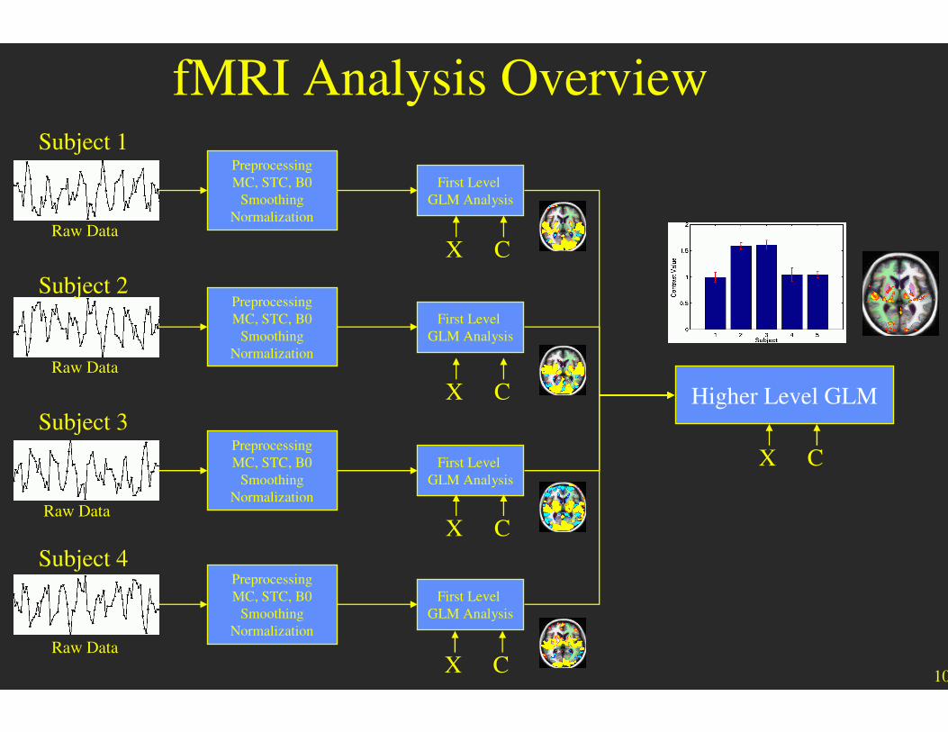
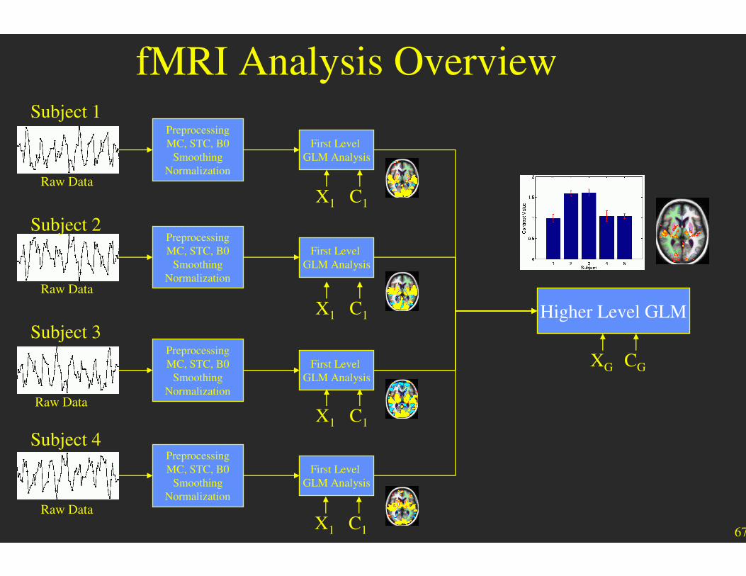
fMRI Analysis Overview

Higher Level GLM

First Level

GLM Analysis

First Level

GLM Analysis

Subject 3

First Level

GLM Analysis

Subject 4

First Level

GLM Analysis

Subject 1

Subject 2

CX

CX

CX

CX

Preprocessing

MC, STC, B0

Smoothing

Normalization

Preprocessing

MC, STC, B0

Smoothing

Normalization

Preprocessing

MC, STC, B0

Smoothing

Normalization

Preprocessing

MC, STC, B0

Smoothing

Normalization

Raw Data

Raw Data

Raw Data

Raw Data

CX

11

Preprocessing

• Assures that assumptions of the analysis are met

• Time course comes from a single location

• Uniformly spaced in time

• Spatial “smoothness”

• Analysis – separating signal from noise

12

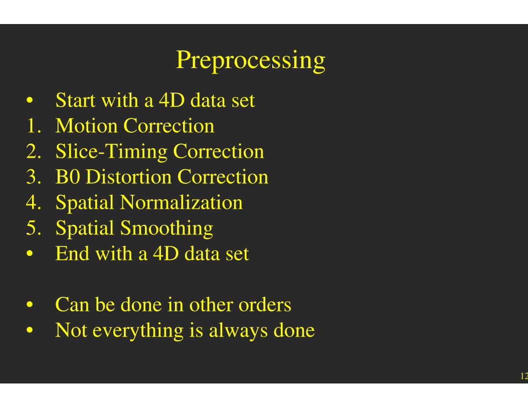
Preprocessing

• Start with a 4D data set

1. Motion Correction

2. Slice-Timing Correction

3. B0 Distortion Correction

4. Spatial Normalization

5. Spatial Smoothing

• End with a 4D data set

• Can be done in other orders

• Not everything is always done

13

Motion

• Analysis assumes that time course represents a

value from a single location

• Subjects move

• Shifts can cause noise, uncertainty

• Edge of the brain and tissue boundaries

14

Motion and Motion Correction

•Motion correction reduces motion

•Not perfect

Raw Corrected

15

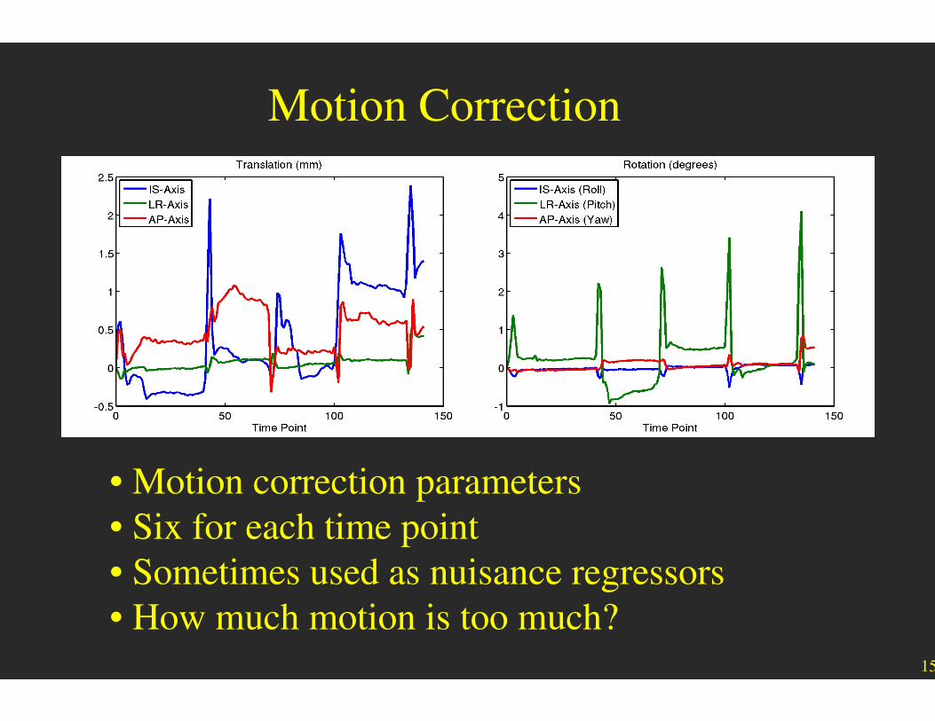
Motion Correction

• Motion correction parameters

• Six for each time point

• Sometimes used as nuisance regressors

• How much motion is too much?

16

Slice Timing

Ascending Interleaved

• Volume not acquired all at one time

• Acquired slice-by-slice

• Each slice has a different delay

• Volume = 30 slices

• TR = 2 sec

• Time for each slice = 2/30 = 66.7 ms

0s

2s

Effect of Slice Delay on Time Course

18

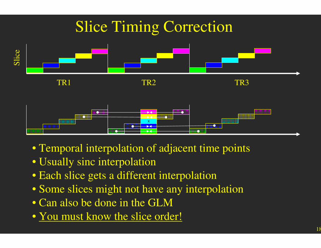
Slice Timing Correction

• Temporal interpolation of adjacent time points

• Usually sinc interpolation

• Each slice gets a different interpolation

• Some slices might not have any interpolation

• Can also be done in the GLM

• You must know the slice order!

X

TR1 TR2 TR3

Sli

ce

19

B0 Distortion

• Metric (stretching or compressing)

• Intensity Dropout

• A result of a long readout needed to get an entire slice in a

single shot.

• Caused by B0 Inhomogeneity

Stretch

Dropout

B0 Map

Echo 2

TE2

Magnitude

Echo 1

TE1

Phase

21

Voxel Shift Map

• Units are voxels (3.5mm)

• Shift is in-plane

• Blue = P�A, Red A�P

• Regions affected near air/tissue boundaries

• sinuses

22

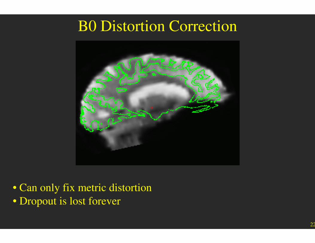
B0 Distortion Correction

• Can only fix metric distortion

• Dropout is lost forever

23

B0 Distortion Correction

• Can only fix metric distortion

• Dropout is lost forever

• Interpolation

• Need:

• “Echo spacing” – readout time

• Phase encode direction

• More important for surface than for volume

• Important when combining from different scanners

24

Spatial Normalization

• Transform volume into another volume

• Re-slicing, re-gridding

• New volume is an “atlas” space

• Align brains of different subjects so that a given voxel

represents the “same” location.

• Similar to motion correction

• Preparation for comparing across subjects

• Volume-based

• Surface-based

• Combined Volume-surface-based (CVS)

25

Spatial Normalization: Volume

Subject 1

Subject 2

Subject 1

Subject 2

MNI305

MNI152

Native Space MNI305 Space

Affine (12 DOF) Registration

26

Subject 1 Subject 2 (Before)

Subject 2 (After) • Shift, Rotate, Stretch

• High dimensional (~500k)

• Preserve metric properties

• Take variance into account

• Common space for group

analysis (like Talairach)

Spatial Normalization: Surface

27

Spatial Smoothing

• Replace voxel value with a weighted average of nearby voxels

(spatial convolution)

• Weighting is usually Gaussian

• 3D (volume)

• 2D (surface)

• Do after all interpolation, before computing a standard deviation

• Similarity to interpolation

• Improve SNR

• Improve Intersubject registration

• Can have a dramatic effect on your results

Spatial Smoothing

Full-Width/Half-max

• Spatially convolve image with Gaussian kernel.

• Kernel sums to 1

• Full-Width/Half-max: FWHM = σ/sqrt(log(256))

σ = standard deviation of the Gaussian

0 FWHM 5 FWHM 10 FWHM

2mm FWHM

10mm FWHM

5mm FWHM

Full Max

Half Max

29

Spatial Smoothing

30

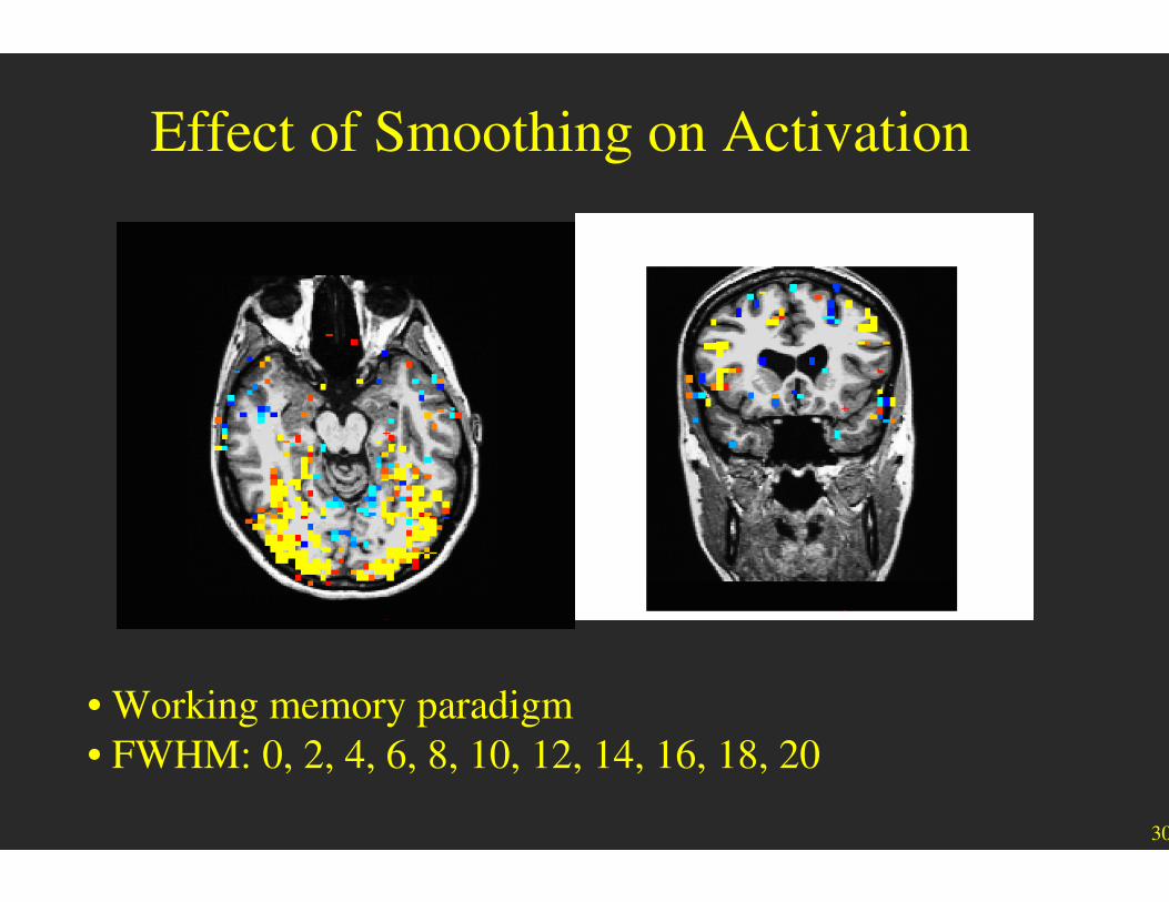
Effect of Smoothing on Activation

• Working memory paradigm

• FWHM: 0, 2, 4, 6, 8, 10, 12, 14, 16, 18, 20

31

Volume- vs Surface-based Smoothing

• 5 mm apart in 3D

• 25 mm apart on surface

• Averaging with other tissue

types (WM, CSF)

• Averaging with other

functional areas

14mm FWHM

32

Preprocessing

• Start with a 4D data set

1. Motion Correction - Interpolation

2. Slice-Timing Correction

3. B0 Distortion Correction - Interpolation

4. Spatial Normalization - Interpolation

5. Spatial Smoothing – Interpolation-like

• End with a 4D data set

• Can be done in other orders

• Not all are done

fMRI Time-Series Analysis

34

fMRI Analysis Overview

Higher Level GLM

First Level

GLM Analysis

First Level

GLM Analysis

Subject 3

First Level

GLM Analysis

Subject 4

First Level

GLM Analysis

Subject 1

Subject 2

CX

CX

CX

CX

Preprocessing

MC, STC, B0

Smoothing

Normalization

Preprocessing

MC, STC, B0

Smoothing

Normalization

Preprocessing

MC, STC, B0

Smoothing

Normalization

Preprocessing

MC, STC, B0

Smoothing

Normalization

Raw Data

Raw Data

Raw Data

Raw Data

CX

35

Visual/Auditory/Motor Activation Paradigm

15 sec ‘ON’, 15 sec ‘OFF’

• Flickering Checkerboard

• Auditory Tone

• Finger Tapping

36

Block Design: 15s Off, 15s On

Voxel 1

Voxel 2

Stimulus Schedule

Paradigm File

37

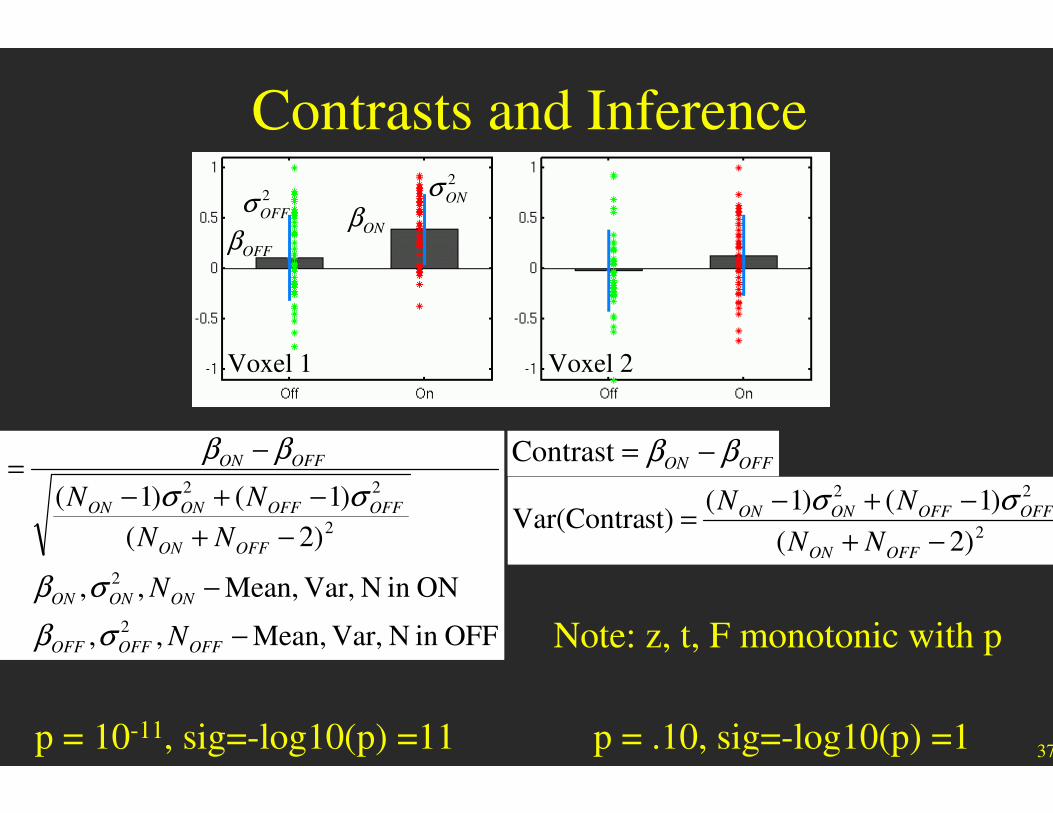
Contrasts and Inference

p = 10-11, sig=-log10(p) =11 p = .10, sig=-log10(p) =1

OFFin N Var, Mean,,,

ONin N Var, Mean,,,

)2(

)1()1(

2

2

2

22

−

−

−+

−+−

−=

OFFOFFOFF

ONONON

OFFON

OFFOFFONON

OFFON

N

N

NN

NNt

σβ

σβ

σσ

ββOFFON ββ −=Contrast

2

22

)2(

)1()1(st)Var(Contra

−+

−+−=

OFFON

OFFOFFONON

NN

NN σσ

ONβOFFβ

2

ONσ2

OFFσ

Voxel 1 Voxel 2

Note: z, t, F monotonic with p

38

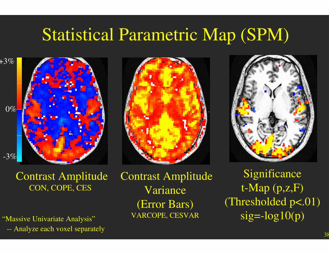
Statistical Parametric Map (SPM)

+3%

0%

-3%

Contrast AmplitudeCON, COPE, CES

Contrast Amplitude

Variance

(Error Bars)VARCOPE, CESVAR

Significance

t-Map (p,z,F)

(Thresholded p<.01)

sig=-log10(p)“Massive Univariate Analysis”

-- Analyze each voxel separately

39

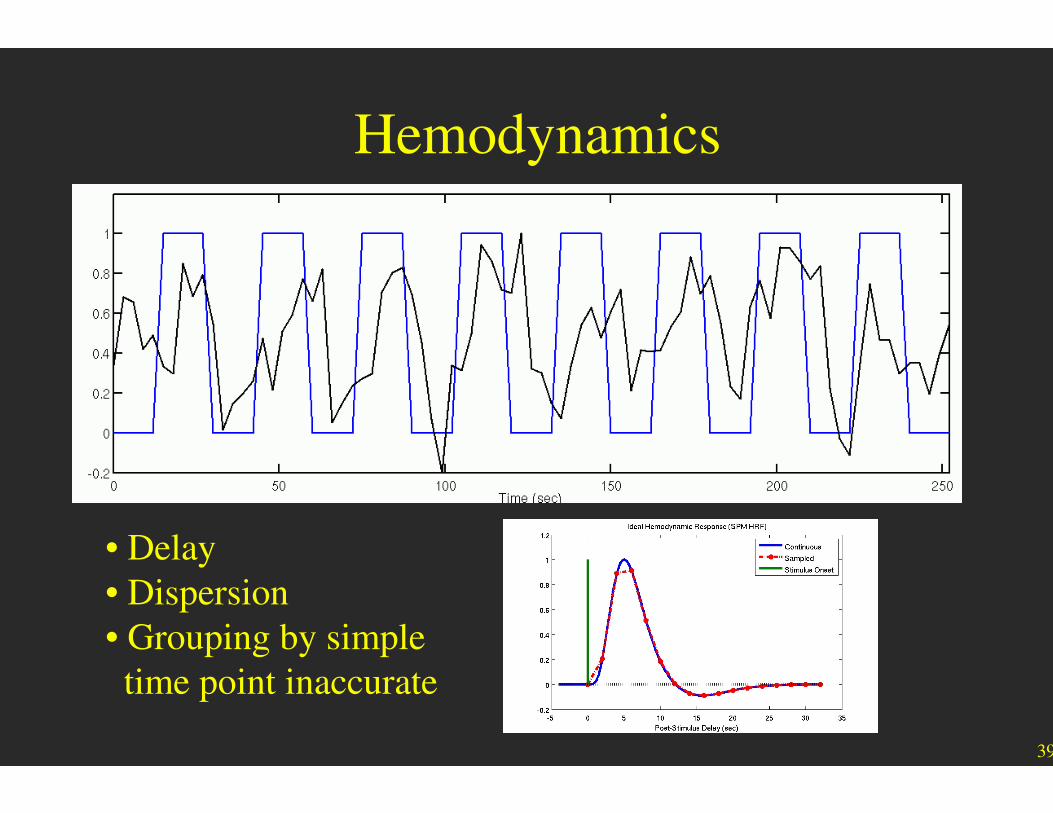
Hemodynamics

• Delay

• Dispersion

• Grouping by simple

time point inaccurate

40

Convolution with HRF

• Shifts, rolls off; more accurate

• Loose ability to simply group time points

• More complicated analysis

• General Linear Model (GLM)

41

GLM

Data fom

one voxel

= βTask βbase+

Baseline Offset

(Nuisance)Task

βTask=βon−βoff•Implicit Contrast

•HRF Amplitude

βbase=βoff

42

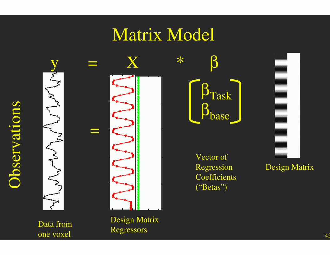
Matrix Model

y = X * β

βTask

βbase

Data from

one voxel

Design Matrix

Regressors

=

Vector of

Regression

Coefficients

(“Betas”)

Design Matrix

Ob

serv

atio

ns

43

Two Task Conditions

y = X * β

βOdd

βEven

βbase

Data from

one voxel

Design Matrix

Regressors

=

Design Matrix

Ob

serv

atio

ns

44

Working Memory Task (fBIRN)

Images Stick Figs

“Scrambled” Encode Distractor Probe

16s 16s 16s 16s

Stick Figs

0. “Scrambled” – low-level baseline, no response

1. Encode – series of passively viewed stick figures

Distractor – respond if there is a face

2. Emotional

3. Neutral

Probe – series of two stick figures (forced choice)

4. Following Emotional Distractor

5. Following Neutral Distractor

fBIRN: Functional Biomedical Research Network (www.nbirn.net)

45

Five Task Conditions

βEncode

βEmotDist

βNeutDist

βEmotProbe

βNeutProbe

=

y = X * β

46

GLM Solution

βEncode

βEmotDist

βNeutDist

βEmotProbe

βNeutProbe

=

y = X * β

• Set of simultaneous equations • Each row of X is an equation

• Each column of X is an unknown

• βs are unknown

• 142 Time Points (Equations)

• 5 unknowns

)(ˆ 1yXXX

TT −=β

47

Estimates of the HRF Amplitude

βEncode

βEmotDist

βNeutDist

βEmotProbe

βNeutProbe

=

Distractor Neutral following Probe toresponsein amplitude cHemodynamiˆ

Distractor Emotional following Probe toresponsein amplitude cHemodynamiˆ

Distractor Neutral toresponsein amplitude cHemodynamiˆ

Distractor Emotional toresponsein amplitude cHemodynamiˆ

Encode toresponsein amplitude cHemodynamiˆ

)(ˆ ,

NeuttProbe

EmotProbe

NeutDist

EmotDist

Encode

1

=

=

=

=

=

=+= −

β

β

β

β

β

ββ yXXXnXyTT

48

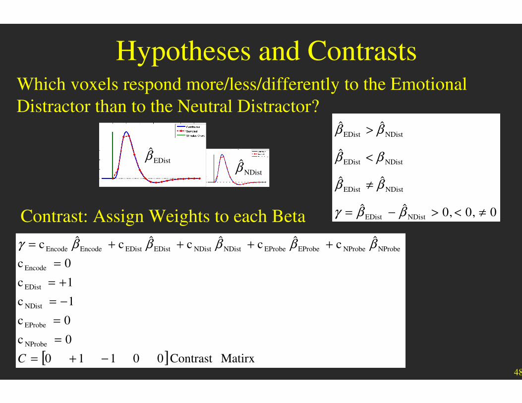
Hypotheses and ContrastsWhich voxels respond more/less/differently to the Emotional

Distractor than to the Neutral Distractor?

0,0,0ˆˆ

ˆˆ

ˆ

ˆˆ

NDistEDist

NDistEDist

NDistEDist

NDistEDist

≠<>−=

≠

<

>

ββγ

ββ

ββ

ββ

[ ] MatirxContrast 00110

0c

0c

1c

1c

0c

ˆcˆcˆcˆcˆc

NProbe

EProbe

NDist

EDist

Encode

NProbeNProbeEProbeEProbeNDistNDistEDistEDistEncodeEncode

−+=

=

=

−=

+=

=

++++=

C

βββββγ

Contrast: Assign Weights to each Beta

EDistβ̂NDistβ̂

49

Hypotheses

• Which voxels respond more to the Emotional Distractor

than to the Neutral Distractor?

• Which voxels respond to Encode (relative to baseline)?

• Which voxels respond to the Emotional Distractor?

• Which voxels respond to either Distractor?

• Which voxels respond more to the Probe following the

Emotional Distractor than to the Probe following the

Neutral Distractor?

50

Which voxels respond more to the Emotional Distractor than to

the Neutral Distractor?

1.

En

cod

e

2.

ED

ist

3. N

Dis

t

4.

EP

rob

e

5. N

Pro

be

• Only interested in Emotional and Neutral Distractors

• No statement about other conditions

Condition: 1 2 3 4 5

Weight 0 +1 -1 0 0

Contrast Matrix

C = [0 +1 -1 0 0]

51

Contrasts and the Full Model

( )

( )ate)(multivariTest -F ˆˆˆF

e)(univariatTest - tˆ)(

ˆ

ˆ

ˆt

Cin Rows J

Estimate VarianceContrast ˆ)(1ˆˆ

Contrast ˆˆ

ˆˆ Variance, Residual ˆˆ

ˆ

EstimatesParameter )(ˆ

),0(~ , ,

1

JDOF,

21DOF

212

2

1

2

γγ

σ

β

σ

γ

σσ

βγ

βσ

β

σβ

γ

γ

γγ

−

−

−

−

Σ=

==

=

=Σ=

=

−==

=

+=+=

T

n

TT

n

TT

T

n

TT

n

CXXC

C

CXXCJ

C

XynDOF

nn

yXXX

NnnsynXy

ONβ

OFFβ

2

ONσ2

OFFσ

2

22

)2(

)1()1(

−+

−+−

−=

OFFON

OFFOFFONON

OFFON

NN

NNt

σσ

ββ

52

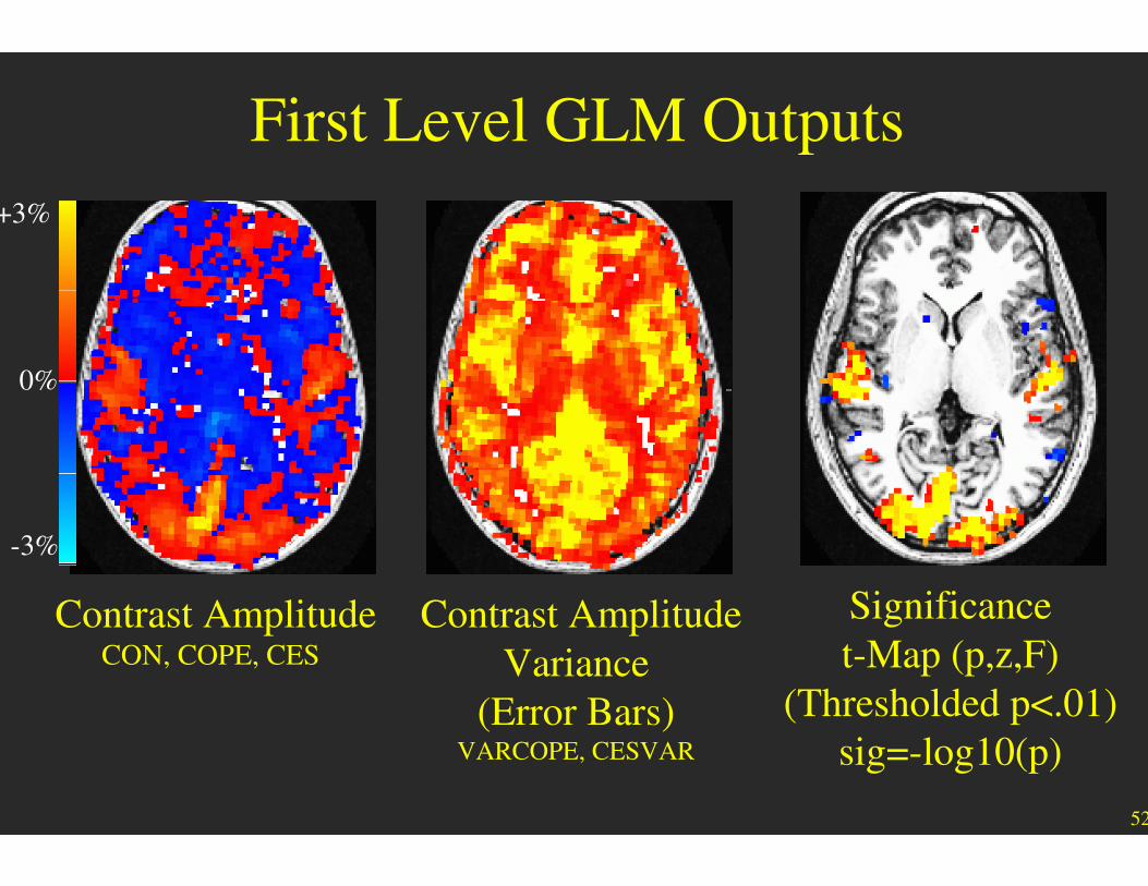
First Level GLM Outputs

+3%

0%

-3%

Contrast AmplitudeCON, COPE, CES

Contrast Amplitude

Variance

(Error Bars)VARCOPE, CESVAR

Significance

t-Map (p,z,F)

(Thresholded p<.01)

sig=-log10(p)

53

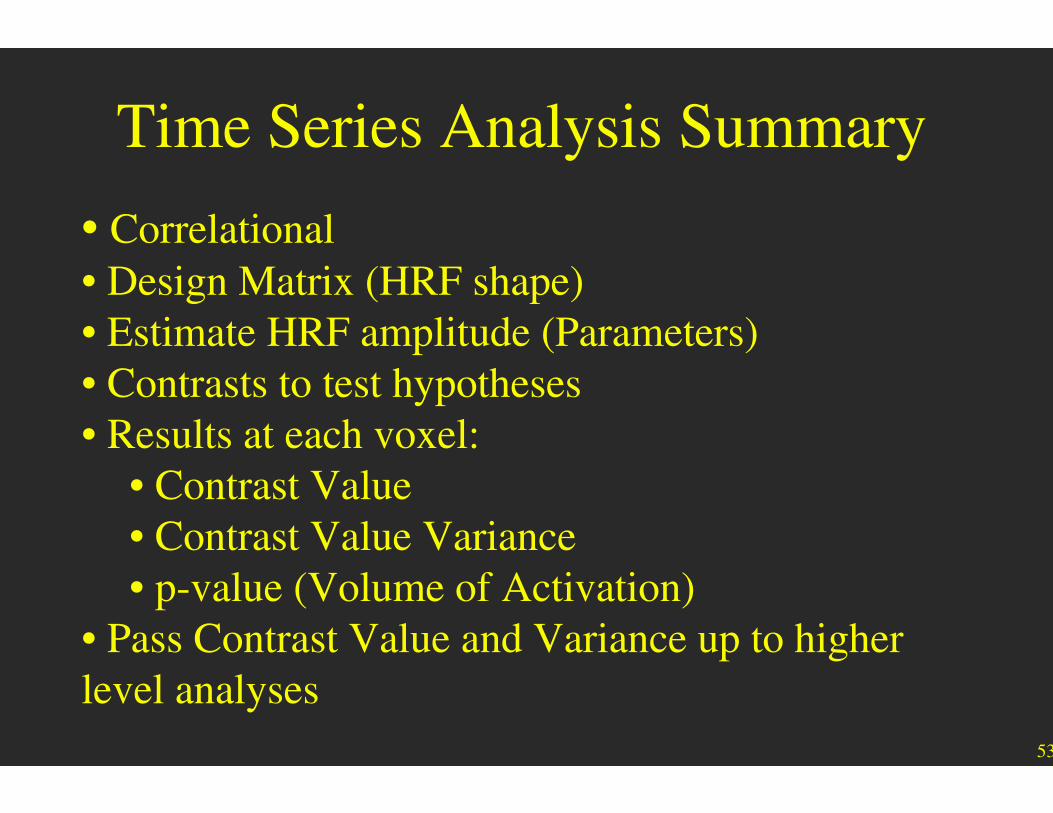
Time Series Analysis Summary

• Correlational

• Design Matrix (HRF shape)

• Estimate HRF amplitude (Parameters)

• Contrasts to test hypotheses

• Results at each voxel:

• Contrast Value

• Contrast Value Variance

• p-value (Volume of Activation)

• Pass Contrast Value and Variance up to higher

level analyses

fMRI Group Analysis

55

fMRI Analysis Overview

Higher Level GLM

First Level

GLM Analysis

First Level

GLM Analysis

Subject 3

First Level

GLM Analysis

Subject 4

First Level

GLM Analysis

Subject 1

Subject 2

CX

CX

CX

CX

Preprocessing

MC, STC, B0

Smoothing

Normalization

Preprocessing

MC, STC, B0

Smoothing

Normalization

Preprocessing

MC, STC, B0

Smoothing

Normalization

Preprocessing

MC, STC, B0

Smoothing

Normalization

Raw Data

Raw Data

Raw Data

Raw Data

CX

56

Overview

• Goal of Group Analysis

• Types of Group Analysis

– Random Effects, Mixed Effects, Fixed Effects

• Multi-Level General Linear Model (GLM)

57

Spatial Normalization, Atlas Space

Subject 1

Subject 2

Subject 1

Subject 2

MNI305

Native Space MNI305 Space

Affine (12 DOF) Registration

58

Inter-Subject Averaging

Subje

ct 1

Subje

ct 2

NativeSpherical Spherical

Surface-to-

Surface

Surface-to-

Surface

GLM

Demographics

cf. Talairach

59

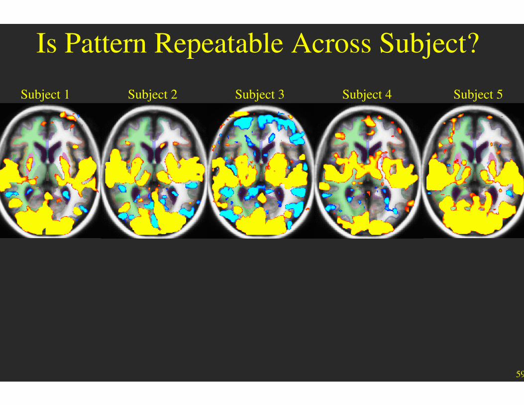
Is Pattern Repeatable Across Subject?

Subject 1 Subject 2 Subject 3 Subject 4 Subject 5

60

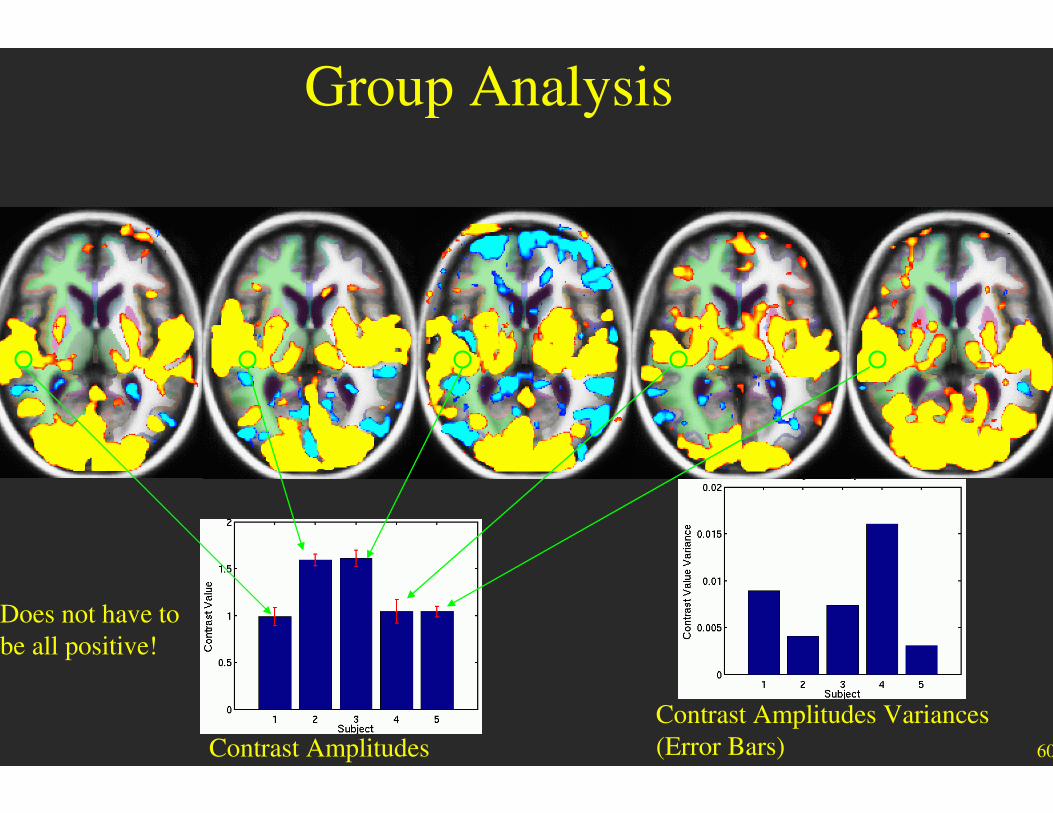
Group Analysis

Does not have to

be all positive!

Contrast Amplitudes

Contrast Amplitudes Variances

(Error Bars)

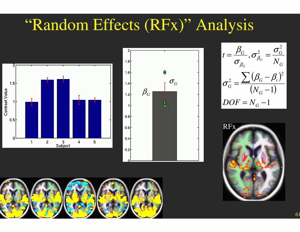
61

GβGσ ( )

( )1

1

,

2

2

22

−=

−

−=

==

∑

G

G

iG

G

G

GG

NDOF

N

Nt

G

G

ββσ

σσ

σ

ββ

β

“Random Effects (RFx)” Analysis

RFx

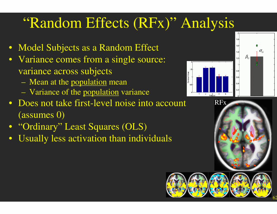
62

Gβ

Gσ

“Random Effects (RFx)” Analysis

RFx

• Model Subjects as a Random Effect

• Variance comes from a single source:

variance across subjects – Mean at the population mean

– Variance of the population variance

• Does not take first-level noise into account

(assumes 0)

• “Ordinary” Least Squares (OLS)

• Usually less activation than individuals

63

“Mixed Effects (MFx)” Analysis

MFx

RFx

• Down-weight each subject based on variance.

• Weighted Least Squares vs (“Ordinary” LS)

64

“Mixed Effects (MFx)” Analysis

MFx

• Down-weight each subject based on variance.

• Weighted Least Squares vs (“Ordinary” LS)

• Protects against unequal variances across group or

groups (“heteroskedasticity”)

• May increase or decrease significance with respect to

simple Random Effects

• More complicated to compute

• “Pseudo-MFx” – simply weight by first-level

variance (easier to compute)

65

“Fixed Effects (FFx)” Analysis

FFx

RFx

( )

∑

∑

=

=

=

i

G

i

G

DOFDOF

N

t

G

G

2

2

2

2

σσ

σ

β

β

β

2

iσ

66

“Fixed Effects (FFx)” Analysis

FFx

( )

∑

∑

=

=

=

i

G

i

G

DOFDOF

N

t

G

G

2

2

2

2

σσ

σ

β

β

β

• As if all subjects treated as a single subject (fixed effect)

• Small error bars (with respect to RFx)

• Large DOF

• Same mean as RFx

• Huge areas of activation

• Not generalizable beyond sample.

67

fMRI Analysis Overview

Higher Level GLM

First Level

GLM Analysis

First Level

GLM Analysis

Subject 3

First Level

GLM Analysis

Subject 4

First Level

GLM Analysis

Subject 1

Subject 2

C1X1

C1X1

C1X1

C1X1

Preprocessing

MC, STC, B0

Smoothing

Normalization

Preprocessing

MC, STC, B0

Smoothing

Normalization

Preprocessing

MC, STC, B0

Smoothing

Normalization

Preprocessing

MC, STC, B0

Smoothing

Normalization

Raw Data

Raw Data

Raw Data

Raw Data

CGXG

68

GβGσ

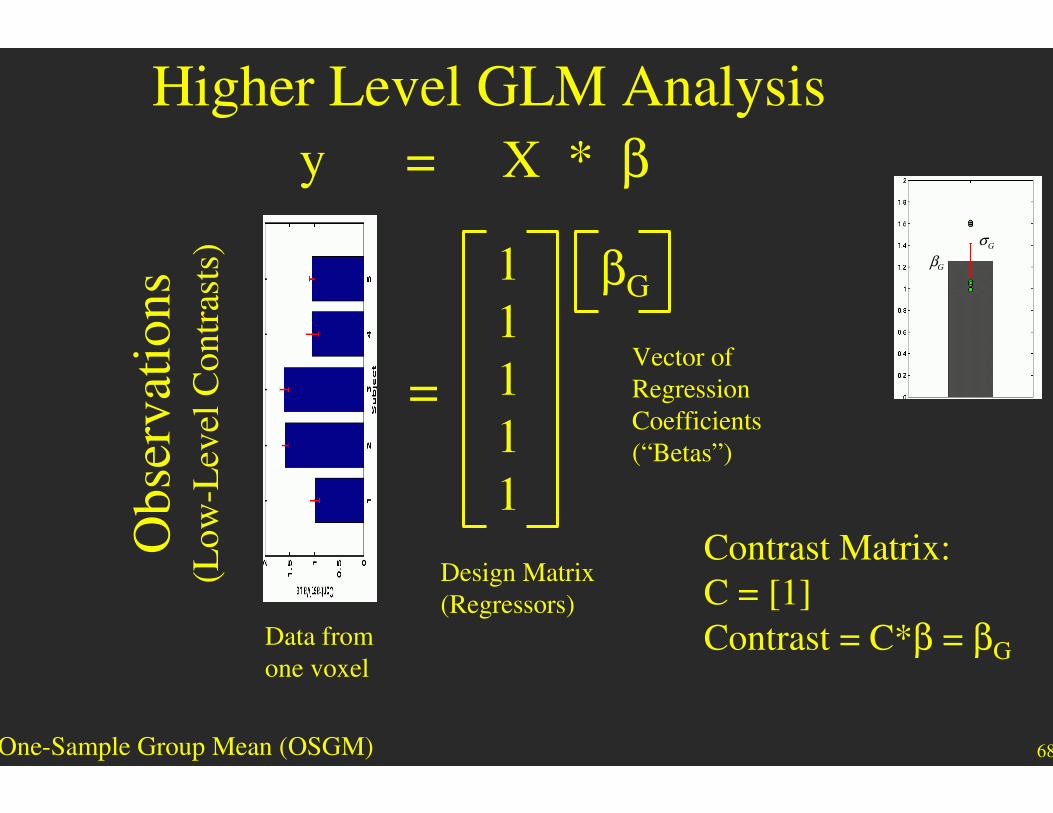
Higher Level GLM Analysis

=

1

1

1

1

1

βG

y = X * β

Data from

one voxel

Design Matrix

(Regressors)

Vector of

Regression

Coefficients

(“Betas”)

Ob

serv

atio

ns

(Lo

w-L

evel

Co

ntr

asts

)

Contrast Matrix:

C = [1]

Contrast = C*β = βG

One-Sample Group Mean (OSGM)

69

Summary

• Preprocessing – MC, STC, B0, Normalize, Smooth

• First Level GLM Analysis – Design matrix, HRF,

Nuisance

• Contrasts, Hypothesis Testing – contrast matrix

• Group Analysis

– Random, Mixed, Fixed

– Multi-level GLM (Design and Contrast Matrices)