basket option pricing for processes with jumps using ... · pdf filebasket option pricing for...

Politecnico di Torino

Corso di Laurea Magistrale in Ingegneria Matematica

Basket Option Pricingfor Processes with Jumps

Using Sparse Grids and Fourier Transforms

A.A 2014/2015

relatori:

Prof. Luigi Preziosi,

Prof. Raul Tempone,

Fabian Crocce,

Yu-Ho Häppölä

elaborato di laurea di:

Alessandro Iania

matricola 190590

Alessandro Iania

Ringraziamenti

Sto concludendo un percorso che probabilmente non avrei mai portato a

termine con le mie sole forze.

Devo ringraziare il gruppo di KAUST per avermi permesso di scrivere

questa tesi nell'ambito di un'esperienza stimolante, vissuta in un'ambiente

internazionale. Grazie dunque a Raul e a Fabian, ma anche ai ragazzi con

cui ho tanto condiviso in questi 7 mesi: Marco, Fuad e tutti gli altri.

La scrittura della tesi è solo la ne di un percorso di crescita molto più

ampio, e sarei cresciuto molto meno senza il contributo costante dei miei

Amici. Gianluca Brero, che mi manca ogni giorno. Matteo Rabagliati, a

cui mi accorgo spesso di aver nito per assomigliare nei miei atteggiamenti:

lo porto con me. Andrea Valenti, così dierente da come sono io, ma a cui

voglio un gran bene. Ferdinando, che ringrazio per essersi fatto scegliere, un

giorno di parecchi anni fa, in una classe di liceo. E poi i compagni di corso,

Veronica, Giri, Erica, Ludo, Simo, Marco, Chiara.

Ai miei genitori, che mi supportano e mi sopportano da ormai 26 anni.

3

Alessandro Iania

Contents

Introduction 6

1 Option Pricing 9

1.1 Denitions . . . . . . . . . . . . . . . . . . . . . . . . . . . . . 9

1.2 Properties of Stock Options . . . . . . . . . . . . . . . . . . . 11

1.2.1 Multidimensional Options: Basket Call Options . . . . 11

1.3 Pricing Background . . . . . . . . . . . . . . . . . . . . . . . . 12

1.3.1 Stochastic Processes . . . . . . . . . . . . . . . . . . . 12

1.3.2 Pricing . . . . . . . . . . . . . . . . . . . . . . . . . . . 13

1.4 Stock Price Models . . . . . . . . . . . . . . . . . . . . . . . . 13

1.4.1 Black Scholes Model . . . . . . . . . . . . . . . . . . . 13

1.4.2 The Variance Gamma Model . . . . . . . . . . . . . . . 16

2 Integration on Sparse Grids 21

2.1 Problem Formulation . . . . . . . . . . . . . . . . . . . . . . . 21

2.2 The Smolyak Method . . . . . . . . . . . . . . . . . . . . . . . 24

2.2.1 Complexity . . . . . . . . . . . . . . . . . . . . . . . . 27

2.2.2 Error Bound . . . . . . . . . . . . . . . . . . . . . . . . 28

3 The Algorithms 31

3.1 Algorithm A: Computing Price using FFT . . . . . . . . . . . 31

3.1.1 One-Dimensional Price . . . . . . . . . . . . . . . . . . 31

3.1.2 (d-1)-Dimensional Integration . . . . . . . . . . . . . . 33

3.1.3 FFT to Compute the (d-1)-Dimensional pdf . . . . . . 33

5

Alessandro Iania

3.1.4 The Code . . . . . . . . . . . . . . . . . . . . . . . . . 36

3.2 Algorithm B: Using the Normality of the CCGM's conditional

pdf . . . . . . . . . . . . . . . . . . . . . . . . . . . . . . . . . 38

3.2.1 The Code . . . . . . . . . . . . . . . . . . . . . . . . . 39

4 Numerical Results 43

4.1 The Importance of the cut-o . . . . . . . . . . . . . . . . . . 44

4.2 A 3-Dimensional Example . . . . . . . . . . . . . . . . . . . . 45

4.2.1 Algorithm A . . . . . . . . . . . . . . . . . . . . . . . . 46

4.2.2 Algorithm B . . . . . . . . . . . . . . . . . . . . . . . . 47


4.3.1 Algorithm A . . . . . . . . . . . . . . . . . . . . . . . . 50

4.3.2 Algorithm B . . . . . . . . . . . . . . . . . . . . . . . . 51


4.4.1 Algorithm A . . . . . . . . . . . . . . . . . . . . . . . . 54

4.4.2 Algorithm B . . . . . . . . . . . . . . . . . . . . . . . . 55

Conclusions 55

Further work 58

Appendices 61

A Matlab Code: Algorithm A 63

B Matlab Code: Algorithm B 71

Introduction

The Common Clock Variance Gamma (CCVG) model, introduced by Madan

and Seneta in the 1990 [15], permits to overcome some of the shortcomings

that aect the typical assumption of log-normal distribution for stock prices

made in the Black-Scholes model [2]. CCVG model has been therefore con-

sidered in the literature to model a set of correlated assets' prices. E. Luciano

and W. Schoutens [13] calibrated this model in the particular case in which

Σ is a diagonal matrix.

We depart from the fundamental theorem of option pricing, which states

that the price of a derivative is the expected income under a particular mea-

sure, the so-called risk-neutral measure. Assuming a risk-neutral measure

given, both algorithms compute this expected income by computing the cor-

responding multidimensional integral using sparse grids. The use of sparse

grids allows us to overcome the curse of dimensionality to a certain extent.

As the sparse grid integration requires a special class of integrand functions,

we manipulate our d-dimensional integral using the law of total expectation

to split it into two parts. Once we obtain a problem formulation that can be

solved using sparse grids, we present two numerical algorithms to compute

our multidimensional integrals. The rst algorithm uses the Fast Fourier

Transform (FFT) to evaluate the (d− 1)-dimensional joint probability den-

sity function. The second algorithm exploits the fact that the CCVG's pdf

conditioned to the random time change (called the clock) has a normal distri-

bution. We describe the two algorithms and we report the numerical results

obtained running them to compute integrals in dierent dimensions. We con-

7

Alessandro Iania

clude the thesis commenting the numerical results and reporting suggestions

for further works.

In this thesis we present two algorithms based on sparse grids to compute

basket options' price under the CCVG model. We introduce the fundamental

concepts needed to fully understand the dissertation, but the reader is still

supposed to be competent in basic probability and measure theory.

A Matlab implementation of the two methods are included respectively

in the Appendix A and in the Appendix B.

Chapter 1

Option Pricing

1.1 Denitions

A derivative can be dened as a nancial instrument whose value derives

from the values of other, more basic, underlying variables. Often the variables

underlying derivatives are the prices of traded assets like stocks. Stocks

are shares in a company which provide partial ownership in the company,

proportional with the investment in the company. They can be bought or

sold at any time time t at a spot price St. All possible future prices St(t),

together with probabilistic information on the likelihood of a particular price

history, constitute the price process S = St : t ≥ 0 of the asset[7].A stock option is a derivative whose value is dependent on the price of a

stock. Its value at expiration time or time to maturity T is determined

by the price process of the option up to time T. The holder of the option has

the right - and not the obligation - to do something. There are several types

of options. A call option gives the holder of the option the right to buy

an asset by a certain expiration date for a certain strike price or exercise

price. A put option is an analogous contract, but the holder has the right

to sell the asset. Call and put options can be either European or American.

AnAmerican option can be exercised at any time until the expiration date,

whereas European options can be exercised only on the expiration date

9

Alessandro Iania

itself. To every option contract there are two sides. On one side there is the

investor who has taken the long position (i.e., he bought the option). On the

other side there is the investor who has taken a short position (i.e., he has

sold or written the option). The writer of an option receives cash up front,

but has potential liabilities later. His prot or loss is the reverse of that for

the purchaser of the option.

The return on an investment is called payo. If K is the strike price and

ST is the nal price of the underlying asset, the payo at time T of a long

position in an European call option is

P (ST ) = max (ST −K, 0) = (K − ST )+

The payo of the analogous put option is (Figure 1.1):

P (ST ) = max (K − ST , 0) = (ST −K)+

Figure 1.1: payo of a put (left) and of a call (right) option with strike

K = 50.

Call options are referred to as in the money when the dierence between

stock price S and strike price K is positive, at the money when S = K, out

of the money when S < K. There are options on stocks, currencies, stock

indices, and futures.

Alessandro Iania

1.2 Properties of Stock Options

The price of a stock option depends on six factors [11]:

The current stock price, S0

The strike price, K

The time to expiration, T

The volatility of the stock price, σ

The risk-free interest rate, r

The dividends that are expected to be paid

The value of a call option generally increases as the current stock price, the

time to expiration, the volatility, and the risk-free interest rate increase, while

it decreases as the strike price and expected dividends increase (Figure 1.2).

1.2.1 Multidimensional Options: Basket Call Options

A call options on a set of stock with component weights c oers its holder

the right to buy the portfolio at a certain strike price K = ek. The payo at

maturity T is therefore

(1.1) P (ST ) = maxc · ST −K, 0 = (c · ST −K)+

The volatility of the basket is generally smaller than that of each un-

derlying. Therefore, the basket option premium is less than the sum of the

premiums of all individual options on each underlying.

Alessandro Iania

00.2

0.40.6

36384042444648500

5

10

15

20

volatilitystrike price K

call

optio

n’s

pric

e

Figure 1.2: price of a call option, evaluated using the B-S formula, depending

on the strike price and on the volatility σ

.

1.3 Pricing Background

1.3.1 Stochastic Processes

Let (Ω,F ,P) be a probability space, and let T be a set of innite cardinality.

If for each t ∈ T there is a random variable St : Ω→ R dened on (Ω,F ,P),

the function S : T ×Ω→ R : S(t, ω) = St(ω) is called a stochastic process

with indexing set T , and is written S = St, t ∈ T .Prices of stocks can be modelled by stochastic processes in continuous time

t ∈ T = [0, T ] where the maturity T is the time horizon. A price model is

said to be arbitrage-free if it is not possible buy and sell a security at two

dierent prices in two dierent markets, making prots without risk.

Alessandro Iania

1.3.2 Pricing

An important result states that a price model is arbitrage free if and only if

there exists an equivalent risk-neutral measure Q ∼ P such that e−∫ t0 r(s)dsSt

is a Q−martingale[20], and therefore

V (S0) = EQ [V(ST , T )]

e−∫ T0 rdt

(see for example [11, chap. 29]). With the hypothesis that r is constant and

the measure Q is given, then the option price at time 0 can be evaluated by

computing

(1.2) V (S0) = e−rTEQ[P (ST , K)]

It is a fundamental result from mathematical nance: under certain model

assumptions, the prices of derivatives can be represented as expected values,

which in turn correspond to high-dimensional integrals (in the case of multi-

dimensional options). Since the integrals can in most cases not be calculated

analytically, they have to be computed numerically. For this scope, two

broad classes of computational methods have emerged: statistical sampling

approach and grid-based methods. In this thesis, we focus on the second

class.

We assume the underlying prices at maturity T to be modelled by

ST = S0e(rT+XT ),

where the random variable XT describes the log-return on forward contracts

to buy stocks at time T.

1.4 Stock Price Models

1.4.1 Black Scholes Model

Denition 1.1. A standard one dimensional Wiener process (also called

Brownian motion) is a stochastic process Wtt≥0 with the following proper-

ties:

Alessandro Iania

W0 = 0

the function t 7−→ Wt is continuous in t

the process Wtt≥0 has stationary, independent increments

the increment Wt+p −Wp has a normal distribution with mean 0 and

variance t, N (0, t).

In the Black-Scholes model, published by F. Black and M. Scholes in 1973

[2], the price process St of the risky asset is modelled by assuming that the

return due to price change in the time interval δt > 0 is

St+δt − StSt

=δStSt

= rδt+ σδWt,

in the limit δt → 0, i.e. that it consists of a deterministic part rδt and a

random part σδWt, where Wt is a Wiener process (Figure 1.3). In the limit

δt→ 0, we obtain the stochastic dierential equation

(1.3) dSt = rStdt+ σdWt, S0 > 0.

Applying the Ito's Lemma to the function G = log(S), it is easy to verify

that log(S) follows a generalized Wiener process with constant drift rate

µ − σ2

2and constant variance rate σ2[11, chap. 13]. The change in log(S)

between times 0 and T is therefore normally distributed, and

(1.4) log(ST ):N[ln(S0) +

(µ− σ2

2

)T, σ2T

]It follows that (1.3) admits the unique solution (see for example [10, pag.7])

St = S0e

(µ−σ

2

2

)t+σWt ,

and that

XT:N(−1

2σ2T, σ2T

).

The same Black and Scholes' assumptions are underlying dierent models

we can nd in literature. However, empirically observed log returns of risky

Alessandro Iania

0 0.2 0.4 0.6 0.8 1 1.2 1.4 1.6 1.8 220

30

40

50

60

70

time t

S(t)

Figure 1.3: Three simulation of stock price's path in the B-S model with

S0 = 40, µ = 0.1, σ = 0.2, T = 2.

assets are not normally distributed but exhibit signicant skewness and kur-

tosis. These empirical facts are not covered by the Black and Scholes model.

Moreover, a Brownian motion has continuous sample paths, when prices are

in reality driven by jumps. Lastly, the model is not able to give realistic

probabilities of extreme events, like crashes and defaults. It is because the

Normal distribution has too light tails, and the model produces continuous

sample paths. The Brownian motion needs a substantial time to reach a low

barrier, where in reality jumps can cause an almost immediate move over the

barrier. Other objections against the log-normal assumption are based on

observed option prices. They are related to the implied volatility (computed

minimizing the distance between observed option prices and those implied

by the B-S model) and are best known under the name volatility smile. The

Black-Scholes model assumes that the implied volatility is constant. As one

computes the implied volatility, it is possible to observe that at a given matu-

Alessandro Iania

rity the volatility seems a non linear function of the strike price K. To correct

the model, in order to capture this behaviour, one strategy is to introduce

jumps in our model by replacing the continuous Brownian motion by a jump

process.

Multidimensional B-S Model

In order to do a multivariate model, a natural way is to consider a vector

of n dependent brownian motions Wt. If Σ = AAT is the constant volatility

matrix, the price process is therefore:

(1.5)dSt

St

= rdt+ AdWt

The random vector XT is then normally distributed

XBST = AWT −

1

2diag(Σ)T : Nd(−

1

2diag(Σ)T,ΣT )

and the characteristic function is

(1.6) φT (z) = e−12T (idiag(Σ)T z+zTΣz).

For details about the multidimensional BS model see for example [20].

The multivariate Gaussian model has some additional shortcomings. Among

these, the fact that the dependence between the assets does not present tail

dependency, and therefore is not realistic.

1.4.2 The Variance Gamma Model

This process was originally introduced by Madan and Seneta (1990) in [15]. It

is a pure jump process, and it introduces jumps, skewness, kurtosis and non-

Gaussian dependence by changing the clock (the random time) of a standard

Brownian motion B(t) by a Gamma process. The Variance Gamma Process

is dened as

Xt = V G(t) = θG(t) + σB(G(t)),

Alessandro Iania

where G(t) is a gamma process and θ is a drift value. It is a positive,

strictly increasing and purely discontinuous Lévy process. In Figure 1.4 are

represented three simulated paths for a stock's price in the VG model.

1 1.1 1.2 1.3 1.4 1.5 1.6 1.7 1.8 1.9 220

40

60

80

100

time t

S(t)

Figure 1.4: Three simulated paths of a stock's price with S0 = 40, σ =

0.2, T = 2, ν = 0.4, θ = 0.03.

Generally the condition E(G(t)) = t is imposed; this normalization con-

dition means that the stochastic clock is not expected to run faster or slower

than the real one. Using this normalization, the density of G(t) can be

written as

(1.7) fG(t)

(x;t

ν,

1

ν

)= x

tν−1 e−

xν

Γ( tν)ν

tν

, ν > 0

where Γ(·) is the gamma function.

Using the fact that V G(t)|G(t) = g has a Gaussian distribution with mean θg

and variance σ2g, it is possible to derive density and characteristic function

Alessandro Iania

of a Brownian motion time changed by the subordinator:

ϕV G(t)(u) = (1− iuνθ +1

2νu2σ2)−

tν ,

(1.8a)

fV G(t)(x) =2e

θxσ2

νtν

√2πσΓ( t

ν)

(x2

2σ2

ν+ θ2

) t2ν− 1

4

K tν− 1

2

(1

σ2

√x2(

2σ2

ν+ θ2)

),

(1.8b)

where K tν− 1

2is the second type modied Bessel function of order t

ν− 1

2

(see [14] for a detailed derivation).

Multidimensional CCVG Model

Let B(t) be a d-dimensional Brownian motion process with covariance rate

Σt and let G(t) denote an univariate gamma process. Than the process

(1.9) X(t) = θG(t) + B(G(t))

is a multivariate gamma process, where θ is a d-dimensional drift vector.The

sources of dependence are two: one is from the stochastic clock, and it means

that all the process jump together. The second one comes from the corre-

lation between Brownian motions, and it means that the amplitude of the

jumps is correlated across assets. Because of the rst source of dependence,

the components of the process remain dependent even if Σ = Id. The CCVG

model in the particular case in which Σ is a diagonal matrix was calibrated

by E. Luciano and W. Schoutens in [13] providing a good t.

The characteristic function of the CCVG is:

(1.10) ϕCCV G(u) = (1− νu′θ +1

2νu′Σu)−

tν .

Even in multidimensional case, considering that X(t)|Gt is a Gaussian ran-

dom vector with mean gθ and variance covariance matrix gΣ, it is possible

to compute the probability density function of the CCVG:

(1.11)

fV G(t)(x) =2ex

′Σ−1θ

νtν (2π)

N2 |Σ| 12 Γ( tν )

(x′Σ−1x

( 2ν + θ′Σ−1θ)

) t2ν−

N4

K tν−

N2

(√(x′Σ−1x)(

2

ν+ θ′Σ−1θ)

),

Alessandro Iania

where K tν−N

2is the second type modied Bessel function of order t

ν− N

2

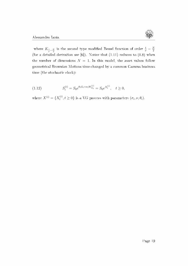
(for a detailed derivation see [6]). Notice that (1.11) reduces to (1.8) when

the number of dimensions N = 1. In this model, the asset values follow

geometrical Brownian Motions time-changed by a common Gamma business

time (the stochastic clock):

(1.12) S(i)i = S0e

θiGt+σiW(i)Gt = S0e

X(i)t , t ≥ 0,

where X(i) = X(i)t , t ≥ 0 is a VG process with parameters (σi, ν, θi).

Alessandro Iania

Chapter 2

Integration on Sparse Grids

2.1 Problem Formulation

Our goal is to price multidimensional options. As expressed in the section 1.3,

we can see the price of a derivative as an expected value; therefore, given a

payo function P (ST ) our purpose is to compute

V (S0) = E (P (ST )) .

In the particular case of a basket call option, dened in subsection 1.2.1, the

expression to compute is:

(2.1) V (S0,K) =

∫Rd

(c · S0ex −K) fXT

(x) dx.

A straightforward method to evaluate multidimensional integrals is to

compound univariate rules coordinate-wise. The problem with this approach

is in the number of function evaluations: the computing cost grows exponen-

tially with the dimension of the problem, since using univariate rules with

N evaluation points results in a d-dimensional quadrature rule with a total

of Nd points. This phenomenon is known as curse of dimensionality, and

it makes the intuitive approach useless even on modern computers for mod-

erately high values of d. Indeed, classical product quadrature methods for

21

Alessandro Iania

the computation of multivariate integrals achieve with n evaluations of the

integrand an accuracy of

ε(n) = O(n−rd )

for functions with bounded derivatives up to order r [1]. For xed r, their

convergence rates rdthus deteriorate as the dimensions increase and are al-

ready in moderate dimensions so small that high accuracies can no longer

obtained in practise. On the positive side, the case r = d indicates that the

problem of high dimensions can sometimes be compensated by, e.g., a high

degree of smoothness. There have been several attempts to overcome the

problem: it is known from numerical complexity theory [19] that some algo-

rithm can break the curse of dimensionality for certain classes of functions.

Monte Carlo (MC) methods are one example of this class of algorithms[3].

Here, the integrand is approximated by the average of n function values at

random points. For square integrable functions f, the expected mean square

error of the Monte Carlo method with n sample is ε(n) = O(n−12 ). The con-

vergence is thus independent of the dimension d, but quite slow.

Under more restrictive assumptions on the smoothness of the integrand,

faster rate of convergence can be attained by deterministic integration meth-

ods such as quasi-Monte-Carlo methods [9] and sparse grid methods[4].

In this thesis we use the Smolyak sparse grid integration to evaluate a multi-

dimensional basket option's price. It is important to notice that the function

we want to integrate in (2.1) is not regular (Figure 2.1).

In order to gain regularity and to make our algorithms converging, it is

convenient to manipulate the expression (2.1). If we set the notation:

S = (S1, . . . , Sd),

S = (S2, . . . , Sd),

s = (s1, . . . , sd) ∈ Rd,

s = (s2, . . . , sd) ∈ Rd−1,

c = (c1, . . . , cd),

Alessandro Iania

−1.5 −1 −0.5 0 0.5 1 1.5 2−2

0

20

100

200

300

X1(T)X2(T)

call’

spa

yoff

Figure 2.1: the payo is not a regular function

c = (c2, . . . , cd),

and we set an analogous notation for X = log STS0, then we can write1:

(2.2)

E(

(c · ST −K)+)

= E

c1S1T −

(K − c · ST

)︸︷︷︸

K′

+

= E(E((

c1S1T −K ′(c, ST ))+∣∣∣∣ ST))

=

∫Rd−1

(∫(c1S10e

x −K ′)+fX1T

(x| XT = x

)dx

)fXT

(x) dx.

It is important to remark that the function

(2.3) xT 7−→∫

(c1S10ex −K ′)+

fX1T

(x| XT = x

)dx

is more regular(Figure 2.2).

1Christian Bayer, personal communication

Alessandro Iania

−1.5 −1 −0.5 0 0.5 1 1.5 2−2

0

20

100

200

300

400

X2(T)X3(T)

pric

e(K

’)

Figure 2.2: the call's price depending on (K,X2T , X3T ) is a regular function

2.2 The Smolyak Method

In the 1963, the Russian mathematician Sergey A. Smolyak introduced a

numerical technique to represent, integrate or interpolate high dimensional

functions. For special function classes, such as spaces of functions which have

bounded mixed derivatives, Smolyak's construction can overcome the curse

of dimensionality to a certain extent. In the original paper [18] the method

was developed for general tensor product spaces. We limit the dissertation

on integrals over regions of Rd, i.e. connected and non-empty subsets, which

may contain some of their boundary points[12].

Let's focus on the function spaces

Hr(Ω) =

f : Ω→ R : ∃ ∂αf(x)

∂xαand is bounded in Ω for all |α|∞ ≤ r

for a region ∅ 6= Ω ⊆ Rdim. r is the regularity of the functions in Hr(Ω), and their

norm is

||f ||Hr(Ω) = maxα∈Nd|α|∞≤r

sup

∣∣∣∣∂αf(x)

∂xα

∣∣∣∣ ; x ∈ Ω

Let's dene two sets Ω and Θ and two linear and bounded functionals:

Alessandro Iania

∅ 6= Ω ⊆ Rd1 ∅ 6= Θ ⊆ Rd2

S : Hr(Ω)→ R T : Hr(Θ)→ RSf =

∑mi=1 aif(xi) T f =

∑ni=1 bif(yi)

⇒ Ω × Θ ⊆ Rd1+d2 and the tensor product of S and T is the linear

functional

S ⊗ T : Hr(Ω×Θ)→ R,

dened by setting:

S ⊗ Tf =m∑i=1

n∑j=1

aibjf(xi, yj).

Let's consider the integral:

(2.4) I dWf =

∫I1

· · ·∫Id

W1(x1) · · ·Wd(xd)f(x1, . . . , xd)dx1, · · · , dxd

Let (U(j)k )dj=1 be a sequence of univariate rules, where k denotes the number of

evaluation points; (w(j)i )

N(j)i=1 and (x

(j)i )

N(j)i=1 are weights and nodes (evaluation

points) of the rule U(j)k .

We can use the univariate rules to coordinate-wise evaluate the integral

(2.4). If we dene

1⊗i=1

U(i)k = U

(1)k and

d⊗i=1

U(i)k =

d−1⊗i=1

U(i)k ⊗ U

(d)k ,

then

I dWf =d⊗i=1

U(i)k f + error.

Let (U(j)i )∞i=1 be a sequence of univariate quadrature rules in the interval

∅ 6= Ij ⊆ R, j = 1, . . . , d. We can dene the dierence operators in Ij:

∆(j)0 = 0, ∆

(j)1 = U

(j)1 and ∆

(j)i+1 = U

(j)i+1 − U (j)

i

The Smolyak quadrature rule of order k in the hyper rectangle I1 × · · · × Idis the operator

Alessandro Iania

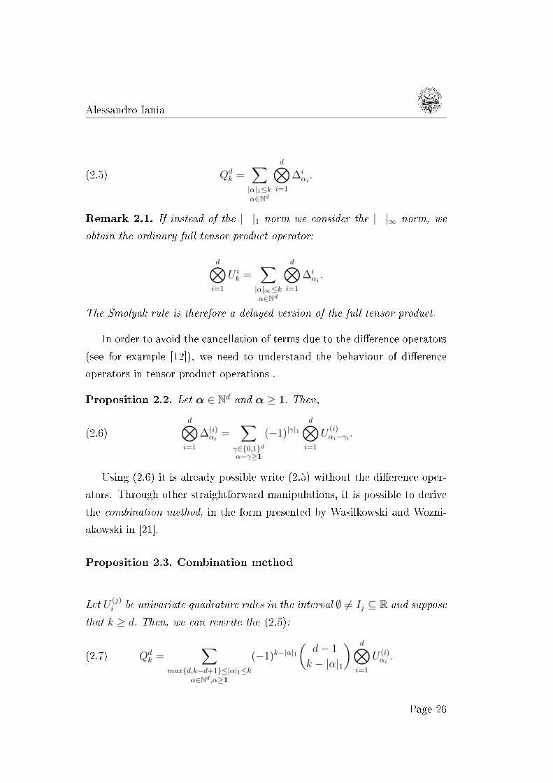
(2.5) Qdk =

∑|α|1≤kα∈Nd

d⊗i=1

∆iαi.

Remark 2.1. If instead of the | |1 norm we consider the | |∞ norm, we

obtain the ordinary full tensor product operator:

d⊗i=1

U ik =

∑|α|∞≤kα∈Nd

d⊗i=1

∆iαi.

The Smolyak rule is therefore a delayed version of the full tensor product.

In order to avoid the cancellation of terms due to the dierence operators

(see for example [12]), we need to understand the behaviour of dierence

operators in tensor product operations .

Proposition 2.2. Let α ∈ Nd and α ≥ 1. Then,

(2.6)d⊗i=1

∆(i)αi

=∑

γ∈0,1dα−γ≥1

(−1)|γ|1d⊗i=1

U(i)αi−γi .

Using (2.6) it is already possible write (2.5) without the dierence oper-

ators. Through other straightforward manipulations, it is possible to derive

the combination method, in the form presented by Wasilkowski and Wozni-

akowski in [21].

Proposition 2.3. Combination method

Let U(j)i be univariate quadrature rules in the interval ∅ 6= Ij ⊆ R and suppose

that k ≥ d. Then, we can rewrite the (2.5):

(2.7) Qdk =

∑maxd,k−d+1≤|α|1≤k

α∈Nd,α≥1

(−1)k−|α|1(

d− 1

k − |α|1

) d⊗i=1

U (i)αi.

Alessandro Iania

We computed the expected value of a basket call option with 5 uncorre-

lated assets using the naive full tensor approach and the Smolyak rule. The

comparison between the rates of convergence is represented in Figure 2.3

0 0.1 0.2 0.3 0.4 0.5 0.6 0.7 0.8 0.9 1 1.1 1.2·106

−5

−4

−3

−2

−1

0

1

2

number of evaluations

rate

ofco

nver

genc

e

Smolyak rulefull tensor approach

Figure 2.3: Comparison of the rate of convergence, dened as the log10 of

the dierence between two consecutive evaluations.

2.2.1 Complexity

(2.7) renders the evaluation points sets on the Smolyak rule explicitly known.

Let U(j)i be a univariate quadrature rules in Ij and let X

(j)i be point sets

containing the respective quadrature rules' evaluation points. Then the eval-

uation points of Qdk, according with (2.7), form the set

η(k, d) =∑

maxd,k−d+1≤|α|1≤kα∈Nd,α≥1

X(1)α1× · · · ×X(d)

αdfor all k ≥ d.

The elements of the set η(k, d) are the nodes of Qdk. The cardinality of the

set η(k, d) is the cost of Qdk, since it is the minimum number of function

Alessandro Iania

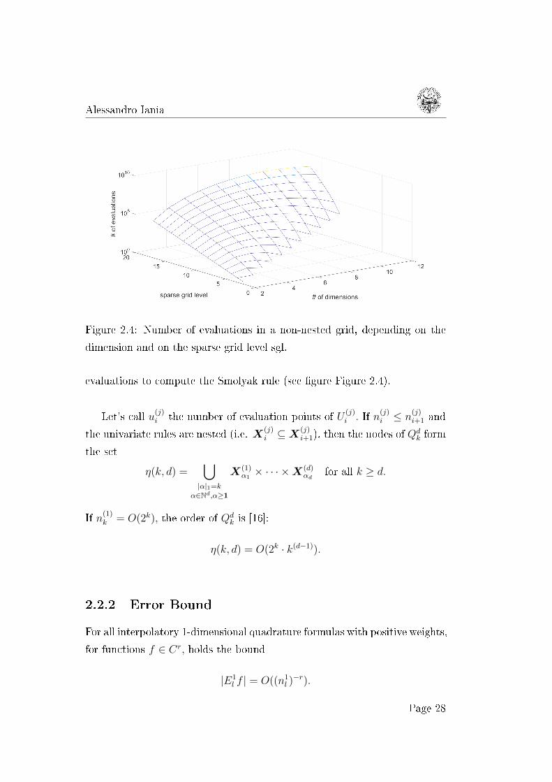
Figure 2.4: Number of evaluations in a non-nested grid, depending on the

dimension and on the sparse grid level sgl.

evaluations to compute the Smolyak rule (see gure Figure 2.4).

Let's call u(j)i the number of evaluation points of U

(j)i . If n

(j)i ≤ n

(j)i+1 and

the univariate rules are nested (i.e. X(j)i ⊆X(j)

i+1), then the nodes of Qdk form

the set

η(k, d) =⋃|α|1=k

α∈Nd,α≥1

X(1)α1× · · · ×X(d)

αdfor all k ≥ d.

If n(1)k = O(2k), the order of Qd

k is [16]:

η(k, d) = O(2k · k(d−1)).

2.2.2 Error Bound

For all interpolatory 1-dimensional quadrature formulas with positive weights,

for functions f ∈ Cr, holds the bound

|E1l f | = O((n1

l )−r).

Alessandro Iania

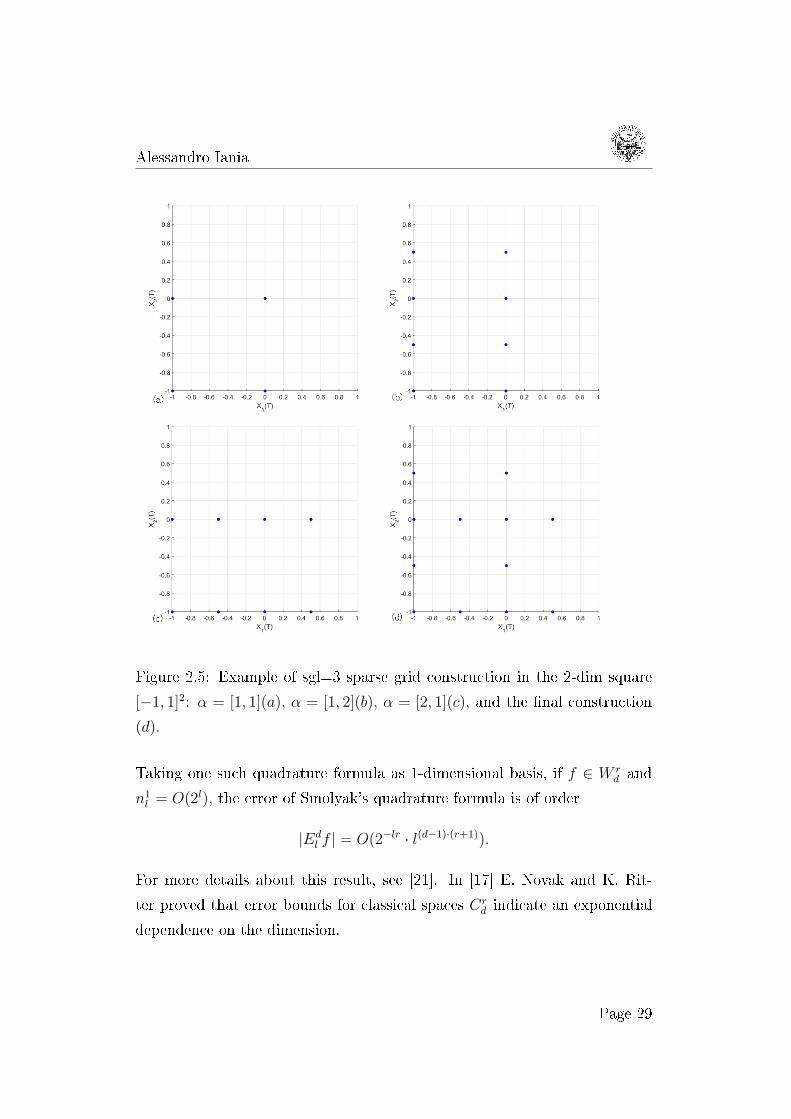
Figure 2.5: Example of sgl=3 sparse grid construction in the 2-dim square

[−1, 1]2: α = [1, 1](a), α = [1, 2](b), α = [2, 1](c), and the nal construction

(d).

Taking one such quadrature formula as 1-dimensional basis, if f ∈ W rd and

n1l = O(2l), the error of Smolyak's quadrature formula is of order

|Edl f | = O(2−lr · l(d−1)·(r+1)).

For more details about this result, see [21]. In [17] E. Novak and K. Rit-

ter proved that error bounds for classical spaces Crd indicate an exponential

dependence on the dimension.

Alessandro Iania

Chapter 3

The Algorithms

As we expressed in section 2.1, in the case of a basket call option our goal is

to compute the integral (2.1):

V (S0, K) =

∫Rd

(c · S0ex −K) fXT

(x) dx.

3.1 Algorithm A: Computing Price using FFT

In order to make our code converging integrating over sparse grid, it is nec-

essary to manipulate the integrand function, increasing its regularity. By a

straightforward manipulation (2.2), we can write:

V (S0, K) =

∫Rd−1

(∫(c1S10e

x −K ′)+fX1T

(x| XT = x

)dx

)fXT

(x) dx.

3.1.1 One-Dimensional Price

We compute the 1-dimensional inner integral

(3.1) O(S10, K) =

∫(c1S10e

x −K ′)+fX1T

(x| XT = x

)dx

using a quadrature formula adapted to the discontinuity D = log(

K′

c1S10

).

In order to evaluate the conditional expected value, we need to compute the

31

Alessandro Iania

normalization coecient:

(3.2) B =

∫ +∞

−∞fXT

(x, x) dx

The result of the computation (3.1) is therefore:

(3.3)

1B·∫ +∞D

fXT(x, x) (c1S10e

x −K ′) dx if K ′ ≥ 0,

1B·(∫ +∞−∞ fXT

(x, x) c1S10exdx)−K ′ if K ′ < 0.

In 3.1.1 are represented the results of (3.3) depending onK ′, in a 2-dimensional

example.

Remark 3.1. Since for the model we discuss in this thesis the pdf decays

faster than the inverse of the payo functions, we can approximate the inte-

grals over an innite regions by cutting the integration region.

−100 −80 −60 −40 −20 0 20 40 600

20

40

60

80

100

120

140

K’

call’

spr

ice

Figure 3.1: price of a 1-dim call option depending on K ′ = K − S20eX2T ,

between X2T = 1.5 and X2T = −1.5.

Alessandro Iania

3.1.2 (d-1)-Dimensional Integration

In order to use the Smolyak rule to compute the integral

(3.4)

∫Rd−1

O(S10,K)fXT(x) dx,

we need to know the probability density function of the (d-1)-dimensional

process, fXT(x). The less expensive way to compute it is by applying the t

to the characteristic function.

Denition 3.2. The characteristic function of the stochastic process XT is

dened by:

(3.5) ϕT (z) = E[eiz

TXT

]=

∫Rdeiz′xpdf(x)dx

Consequently, we can compute the pdf from the characteristic function

ϕ(z):

(3.6) pdf(x) =1

(2π)d

∫Rde−iz

′xϕ(z)dz

3.1.3 FFT to Compute the (d-1)-Dimensional pdf

The d-dimensionaf Fourier transform is dened by

(3.7) F g(x)(z) =

∫ +∞

−∞· · ·∫ +∞

−∞eiz

Txg(x)dx,

where z ∈ Rd. The function g(x) is called Fourier integrable if F g(x)(z)

exists and is analytic for all z ∈ Rd. The inverse Fourier transform is conse-

quently dened by:

(3.8) g(x) =1

(2π)d

∫ +∞

−∞· · ·∫ +∞

−∞e−ix

T zF g(x)(z)dz

Remark 3.3. Because of the scalar product in (3.5), we can apply the inverse

Fourier transform to the d-dimensional characteristic function with input

[0, XT ] and compute the (d-1)-dimensional pdf.

Alessandro Iania

Let's focus on the 2-dimensional case, and consider the grid

xp = (x0 + p∆x) = (x1p1 , x

2p2) = (x1

0 + p1∆x1, x20 + p2∆x2)

and the corresponding grid in the dual space

zj = (z0 + j∆z) = (z1j1 , z

2j2) = (z1

0 + j1∆z1, z20 + j2∆z2)

If we have the characteristic function ϕ(z) and we want to compute the pdf

value in a node xp, we can write:

pdf(xp) =1

(2π)2

∫R2

e−iz′·xpϕ(z)dz =

1

(2π)2

∫R2

e−i(z1·x1

p1+z2·x2

p2

)ϕ(z1, z2)dz1dz2 =

=1

(2π)2

∫R

n1−1∑j1=0

e−i(z1j1·x1p1

+z2·x2p2

)ϕ(z1

j1 , z2)∆z1dz2 =

=1

(2π)2

∫R

n1−1∑j1=0

e−i((z10+j1∆z1)·x1

p1+z2·x2

p2

)ϕ(z1

j1 , z2)∆z1dz2 =

=1

(2π)2

n1−1∑J1=0

e−i(z10+j1∆z1)x1

p1

n2−1∑J2=0

e−i(z20+j2∆z2)x2

p2ϕ(z1j1 , z

2j2

)∆z1∆z2

since, given the vector of indexes from 0 to n− 1 = (n1 − 1, n2 − 1)

j = (j1, j2) and p = (p1, p2),

the bi-dimensional FFT is dened as

(3.9) Xp =n1−1∑j1=0

n2−1∑j2=0

xje(−i2πp·(j./n)),

we can continue writing

pdf(xp) =1

(2π)2

n1−1∑j1=0

e−1(z10+j1∆z1)x1

p1

n2−1∑j2=0

e−1(z20+j2∆z2)x2

p2ϕ(z1j1 , z

2j2

)∆z1∆z2 =

=1

(2π)2

n1−1∑j1=0

e−1(z10+j1∆z1)(x10+p1∆x1)n2−1∑j2=0

e−1(z20+j2∆z2)(x20+p2∆x2)ϕ(z1j1 , z

2j2

)∆z1∆z2

Alessandro Iania

in order to get a sum in the form of (3.9), we are forced to impose the

following condition on the grid spacings:

(3.10) ∆zi∆xi =2π

ni, for i = 1, 2

under this condition, we can continue manipulating our equation, obtaining:

(3.11)

pdf(xp) =1

(2π)2e−i(z′0·xp

)∆z1∆z2

n1−1∑j1=0

n2−1∑j2=0

e−i(j1∆z1x10+j2∆z2x20)·

· e−i(j1p1 2πn1

)e−i(j2p2 2π

n2)︸︷︷︸

e−i2πp·(j./n)

ϕ(z1j1 , z

2j2

)=

=1


)∆z1∆z2

n1−1∑j1=0

n2−1∑j2=0

e−i(j1∆z1x10+j2∆z2x20)ϕ

(z1j1 , z

2j2

)︸︷︷︸factor mpj to which apply the FFT

e−i2πp·(j./n) =

=1


)∆z1∆z2FFTmpj.

−1

0

1

−1

0

1

0

1

2

3

4

5

6

pdf evaluated by FFT

−1

0

1

−1

0

1

0

1

2

3

4

5

6

pdf

−1

0

1

−1

0

1

−1

0

1

2

3

4

5

·10−4

error

Figure 3.2: 2-dimensional CCVG model's pdf

Alessandro Iania

3.1.4 The Code

The algorithm is essentially composed by three main parts, each one with a

certain assignment:

build the sparse grid algorithm

evaluate a full tensor product

compute a unidimensional integral

The implementation results therefore in three principal functions. To make

the writing of the code straightforward, we used a function based on Algo-

rithm 8.1.1 in [8]. Given two number d and l, this function determines all

the d-uples the sum of whose elements is equal to l.

A Matlab implementetion of the code is in Appendix A.

Algorithm 1 basket call option pricing using the 1-dimensional trick and

integrating over sparse gridSparse grid algorithm

Require: sgl, S0, k, r, T, C,model's parameters

1: for l=max(dim-1sgl-dim) to sparse grid level sgl do

2: compute the coe(sgl,dim,l)

3: evaluate all the (dim-1)-uple αi : |αi|1 = l

4: for every αi do

5: if it is not already stored, compute the full tensor product by eval-

uatefulltensor and store it

6: integral ← integral+coe · full tensor product(αi)7: end for

8: end for

9: option's price ←integral

Alessandro Iania

Algorithm 2 evaluates the full tensor product corresponding to α of the

function O(K,S2T , . . . , SdT ) · pdf(S2T , . . . , SdT )

evaluatefulltensor

Require: sgl, S0, K, r, T, C,model's parameters

build the grids with N = 2α(i) nodes in every dimension in the real space

and in the Fourier one, with the condition ∆z = 2π/n. ·∆x2: ] = prod(n) number of points in each grid

for j=1:] do

4: if the 1-dimensional integral is still to be computed then

compute it by oneintegral and store it

6: end if

M(j)← ϕ(0,xj) · e−izj ·x0

8: SUPP(j)← 1(2π)d·prod(∆z) ·e−iz0·xj ·1-dimensional integral ·prod(∆x)

end for

10: fulltensor=sum(SUPP. · (fft(M)))(:)

Algorithm 3 given the dim-1 nal components corresponding to the node

xj, this function computes the corresponding call's price, considering the new

K' and the model's parameters.oneintegral

Require: S0, K, r, T, C,model's parameters

K ′ = K −∑dimj=2 CjXj

if K ′ > 0 then

oneprice=E (C1S1T −K ′)+adapting the integration to the discontinuity D

else

oneprice=(C1E(S1T )−K ′)end if

Alessandro Iania

3.2 Algorithm B: Using the Normality of the

CCGM's conditional pdf

As expressed in section 1.4.2, in a CCVG process the random vector X(t)|Gt =

g is Gaussian with mean gθ and variance covariance matrix gΣ. Therefore

the density of X(t) can be obtained integrating:

(3.12) CCV Gpdf (X; ν,Σ, θ) =

∫ +∞

0

Npdf (X; θg, gΣ)fgamma

(g;t

ν,

1

ν

)dg.

Given a payo function P (XT ), we can embed the equation (3.12) in (2.1)

and write:

V (X0) =

∫Rd

P (x) · CCV Gpdf(x)dx =

=

∫Rd

P (x) ·∫ +∞

0

Npdf (x; θg, gΣ)fgamma

(g;t

ν,

1

ν

)dgdx =

=

∫ +∞

0

∫Rd

P (x) · Npdf (x; θg, gΣ)dxfgamma

(g;t

ν,

1

ν

)dg.

The embedded d-dimensional integral is computed splitting it into two part as

in the previous algorithm, with the dierence that now the probability density

function has a normal distribution. In this case we know analytically either

the conditional 1-dimensional pdf and the (d-1)-dimensional pdf. Moreover,

it is possible do derive a closed expression for the two cases in algorithm 3.

For example, if we want to consider a basket call's payo, we can name

w = logK ′

C1S10

and evaluate analytically the payo's expected value, in the case K ′ > 0:

(3.13)

∫ +∞

w

1

σ√

2πe−

(x−µ)2

2σ2 (C1S10ex −K ′) dx =

= K ′ (φ(K ′, µ, σ)− 1) +

∫ +∞

w

C1S10ex 1

σ√

2πe−

(x−µ)2

2σ2 dx =

= K ′ (φ(K ′, µ, σ)− 1) + C1S10eσ2+2µ

2

∫ +∞

w

1

σ√

2πe−

(x−(µ+σ2)2

2σ2 dx =

= K ′ (φ(K ′, µ, σ)− 1) + C1S10eσ2+2µ

2

(1− φ

(K ′, µ+ σ2, σ

)).

Alessandro Iania

Analogously, in the case K ′ ≤ 0 we can write:

(3.14)

−K ′ +∫ +∞

−∞

1

σ√

2πe−

(x−µ)2

2σ2 C1S10exdx =

= −K ′ + C1S10eσ2+2µ

2

∫ +∞

−∞

1

σ√

2πe−

(x−(µ+σ2))2

2σ2 exdx = −K ′ + C1S10eσ2+2µ

2 .

3.2.1 The Code

The algorithm embeds the one described in subsection 3.1.4. It includes the

three main parts:

build the sparse grid algorithm

evaluate full tensor product

compute a unidimensional integral

The rst one corresponds to algorithm 5, while in the other two parts the

implementation take in account that now the multidimensional density is

normal, and therefore we don't need to apply the FFT to the characteristic

function anymore.

Algorithm 4 basket call option pricing computing 1-dimensional grid's val-

ues integrating over sparse grid.CCVG pricing algorithm


discretize the gamma function's support in ]g points

for i=1:]g do

g(i)=gammapdf(gi,Tν

1ν)

p(i)=sparsegridalgo(sgl,S0, K, r, SIGMA. ∗ gi,,T,C,gi. ∗ θ)end for

option's price=quadraturerule(g(i),p(i))

Alessandro Iania

Algorithm 5 basket call option pricing using the 1-dimensional trick and

integrating over sparse gridSparse grid algorithm


1: for l=max(dim-1,sgl-dim) to sparse grid level sgl do

2: compute the coe(sgl,dim,l)

3: evaluate all the (dim-1)-uple αi : |αi|1 = l

4: for every αi do

5: if it is not already stored, compute the full tensor product by eval-

uatefulltensor and store it

6: integral ← integral+coe · full tensor product(αi)7: end for

8: end for

9: option's price =integral

Algorithm 6 evaluates the full tensor product corresponding to α of the

function O(K,S2T , . . . , SdT ) · pdf(S2T , . . . , SdT )

evaluatefulltensor

Require: α, sgl, S0, K, r, T, C,model's parameters

Ensure: full tensor product

build the grid with n = 2α(i) nodes in every dimension i=1, · · · , dim− 1:

] = prod(n) number of grid's points

for j=1:] do

M(j)← pdf(xj)· oneintegral (xj, K,model's parameters)

end for

fulltensor=sum(M(:))

Alessandro Iania

Algorithm 7 given the dim-1 nal components corresponding to the node

xj, this function computes the corresponding call's price, considering the new

K' and the model's parameters.oneintegral

Require: S0, K, r, T, C,model's parameters

K ′ = K −∑dimj=2 CjXj

compute the conditioned 1-dimensional µ

compute the conditioned 1-dimensional σ

if K ′ > 0 then

oneprice is computed by (3.13)

else

oneprice is computed by (3.14)

end if

Alessandro Iania

Chapter 4

Numerical Results

In this chapter we show the outputs of the two algorithms presented in chap-

ter 3. Although the second algorithm embeds the rst one, it is quite dicult

to make a fair comparison. In fact, in the rst one every evaluation is very

expensive, while in Algorithm B the closed formulas reported in (3.3) make

the computation quite faster. On the other hand, in Algorithm B there are

some inputs parameters, not present in Algorithm A, that can compromise

the quality of the rate of convergence. Besides, Algorithm A is more opti-

mised, as it includes hashmaps for direct access to already computed data

and a more sophisticated parallelization of the code has been implemented.

In Figure 4.1 is shown a comparison between the running time of Algorithm

A in a 3-dimensional case and the time that Algorithm B needs to compute

a 3-dimensional integral in a single 1-dimensional point.

Given that we did not include in this thesis an analysis of the errors in the

two algorithms, we refer to a reference value, computed either "overkilling

the algorithm" and running a Monte Carlo simulation for an amount of time

such that we can reasonably trust the result.

We run the codes in dierent dimensions. In the 3-dimensional and in the

5-dimensional cases we give as inputs the parameters of the model tted by

Luciano and Schoutens in [13].

43

Alessandro Iania

13 14 15 16 17101

102

103

104

sparse grid level

runn

ing

time

(s)

Algorithm 1Agorithm 2 in a point

Figure 4.1: comparison between the running time in a 3-dimensional analo-

gous computation.

4.1 The Importance of the cut-o

As we mentioned in 3.1, we can approximate the exact result of the inte-

gration by integrating in a (d-1)-dimensional hyperrectangle. Neverthless, it

is very important, in order to obtain a good result and a good rate of con-

vergence, to choose properly the cut-o. It is a common aspect in the two

algorithms, and it is illustrated in Figure 4.2.

Alessandro Iania

5 10 15 20 25 30 35−5

−4

−3

−2

−1

0

n ∝ cut−o f fσ

log 1

0(|re

fere

nce

valu

e−co

mpu

ted

valu

e|)

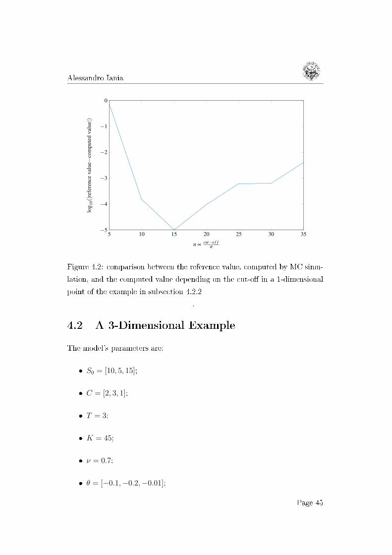
Figure 4.2: comparison between the reference value, computed by MC simu-

lation, and the computed value depending on the cut-o in a 1-dimensional

point of the example in subsection 4.2.2

.

4.2 A 3-Dimensional Example

The model's parameters are:

S0 = [10, 5, 15];

C = [2, 3, 1];

T = 3;

K = 45;

ν = 0.7;

θ = [−0.1,−0.2,−0.01];

Alessandro Iania

Σ =

0.12 0.036 0.018

0.036 0.27 0.0405

0.018 0.0405 0.27

4.2.1 Algorithm A

Chosen a cut-o value, the result of the computation goes towards the refer-

ence value (computed overkilling Algorithm B and corroborating the result

running a MC simulation) as the sparse grid level increases. The log10 of the

absolute value of the dierence between the two evaluations is represented

in Figure 4.3 depending on the sparse grid level sgl. It is possible to observe

that the cut-o we chose to run the code makes every computation with a

sparse grid level higher that 13 essentially useless. How the running time is

related with the sparse grid level is represented in Figure 4.4.

7 8 9 10 11 12 13 14 15−4.5

−4

−3.5

−3

−2.5

−2

−1.5

−1

−0.5

sparse grid level

log 1

0(|re

fere

nce

valu

e−co

mpu

ted

valu

e|)

Figure 4.3: comparison between the reference value and the computation,

depending on the sparse grid level sgl.

Alessandro Iania

13 14 15 16 17102

103

104

sparse grid level

runn

ing

time

(s)

Figure 4.4: the running time grows exponentially as the sparse grid level

increases.

4.2.2 Algorithm B

Algorithm B requires to compute a multidimensional integral in every node of

a 1-dimensional grid. These values are then used to compute a 1-dimensional

integral. In Figure 4.5 is represented the convergence rate in a single 3-

dimensional computation, corresponding to a 1-dimensional node.

The quality of the whole result can be improved both by adding points in

the 1-dimensional computation (and therefore evaluating more d-dimensional

integrals) and by increasing the number of nodes in the computation evalu-

ated in every point. In Figure 4.6 is represented how the result steers towards

the reference value as the number of points increases. On the other hand,

Figure 4.7 shows how increasing the sparse grid level aects the results, keep-

ing the number of 1-dimensional points xed.

Figure 4.8 shows how both the sparse grid level in every 1-dimensional point

and the number of 1-dimensional integration points aects the time needed

in the whole computation.

Alessandro Iania

6 7 8 9 10 11 12 13 14 15 16−12

−10

−8

−6

−4

−2

0

2

sparse grid level

rate

ofco

nver

genc

e

Figure 4.5: rate of convergence in a single point, dened as the log10 of

the dierence of two consequent computations, depending on the sparse grid

level.

12 24 36 48 60−3.5

−3

−2.5

−2

−1.5

−1

number of points in the 1-dimensional discretization

log 1

0(|re

fere

nce

valu

e−co

mpu

ted

valu

e|)

Figure 4.6: comparison between the computed price and the reference one

increasing the number of points, keeping sgl=9.

Alessandro Iania

6 7 8 9 10 11 12 13 14 15−10

−8

−6

−4

−2

0

sparse grid level in every 1-dim integration point

log 1

0(|re

fere

nce

valu

e−co

mpu

ted

valu

e|)

Figure 4.7: comparison between reference value (computed overkilling the

algorithm) and computed value increasing the sgl in 60 integration points.

7 8 9 10 11 12 13 14 15

1224

3648

60100

101

102

103

104

sparse grid level

# of points in the 1-dim integral

runn

ing

time

(s)

Figure 4.8: running time vs sparse grid level in every point vs number of

points.

Alessandro Iania



S0 = [5, 6, 10, 9, 11];

C = [1, 1, 2, 1, 1];

T = 2;

K = 47;

ν = 0.4;

θ = [−0.03,−0.02,−0.01,−0.02,−0.03];

Σ =

0.08 0.012 0.0006 0 0

0.012 0.045 0 0 0

0.0006 0 0.002 0 0

0 0 0 0 0.00648

4.3.1 Algorithm A

The reference value has been computed running a MC simulation for several

hours.

As we can see in Figure 4.9, in 5 dimensions we already need a high sparse

grid level to obtain a value near to the reference one. Moreover, choose the

right cut-o becomes increasingly more important. In general, the Monte

Carlo simulation is already less expensive than the algorithm, as the sgl=13

computation takes around 3.4 hours.

Alessandro Iania

11 12 13 14 15−3

−2.5

−2

−1.5

−1

−0.5

sparse grid level

log 1

0(|re

fere

nce

valu

e−co

mpu

ted

valu

e|)

Figure 4.9: comparison of the computed value with the reference one, de-

pending on the sparse grid level sgl, in a 5-dimensional simulation.

4.3.2 Algorithm B

As in the 3-dimensional example, we can steer towards the reference result

both increasing the number of nodes to discretize the 1-dimensional interval

(Figure 4.10) or increasing the sparse grid level in every point (Figure 4.11).

The running time of the algorithm depending on the number of points used

to discretize the 1-dimensional interval and on the sgl is represented in Fig-

ure 4.12. This algorithm reveals to be faster than the Monte Carlo simulation

even in a 5-dimensional example, as we need to run the MC simulation for

4.5 hours (computed in parallel using 12 cores) to obtain a result x : the

exact x ∈ (x− 0.0004, x+ 0.0004) with a condence of the 99%.

Alessandro Iania

12 24 36 48 60−4.5

−4

−3.5

−3

−2.5

−2

−1.5

−1

−0.5


log 1

0(|re

fere

nce

valu

e−co

mpu

ted

valu

e|)

Figure 4.10: comparison with the reference value increasing the number of

points, keeping sgl=14.

6 7 8 9 10 11 12 13

−3

−2

−1

0

1

sgl in every 1-dim integration point

log 1

0(|re

fere

nce

valu

e−co

mpu

ted

valu

e|)

Figure 4.11: comparison with the reference value increasing the sgl in 48

integration points.

Alessandro Iania

910

1112

1314

12

24

36

48101

102

103

104

sgl

# of points in the 1-dim integral

runn

ing

time

(s)

Figure 4.12: running time vs sparse grid level in every point vs number of

points.



S0 = [10, 5, 12, 8, 7, 15, 9];

C = [1, 2, 1, 1, 1, 1, 1];

T = 1;

K = 70;

ν = 0.1;

θ = [0.004, 0.002, 0.001, 0.002, 0.003, 0.005, 0.002];

Alessandro Iania

Σ =

0.04 0.006 0 0 0 0 0

0.006 0.009 0 0 0 0 0

0 0 0.009 0 0 0 0

0 0 0 0.04 0 0 0

0 0 0 0 0.001 0 0

0 0 0 0 0 0.04 0.002

0 0 0 0 0 0.002 0.01

4.4.1 Algorithm A

Algorithm A proved to be unable to solve the problem in a reasonable amount

of time, as it is shown in Figure 4.13. The simulation with sparse grid level

13 takes around 6000 seconds, and the method is therefore much less ecient

than a Monte Carlo simulation.

9 10 11 12 13−2.4

−2.2

−2

−1.8

−1.6

−1.4

−1.2

−1

−0.8

−0.6

sparse grid level

log 1

0(|re

fere

nce

valu

e−co

mpu

ted

valu

e|)

Figure 4.13: comparison with the reference MC value and the computation,

depending on the sparse grid level sgl, in a 7-dimensional simulation.

Alessandro Iania

4.4.2 Algorithm B

Even Algorithm B reveals to be unsuitable to compute the 7-dimensional

problem. Either adding number of points in the 1-dimensional grid (Fig-

ure 4.14) or increasing the sparse grid level in every points (Figure 4.15),

we are not able to obtain a satisfying result in a reasonable time. These

verications lead to our suggestions about the further works.

6 12 18 24−1.6

−1.55

−1.5

−1.45

−1.4

−1.35

−1.3

−1.25

−1.2


log 1

0(|re

fere

nce

valu

e−co

mpu

ted

valu

e|)

Figure 4.14: comparison between the MC evaluated value and the computed

one, increasing the number of points with sgl=14.

Alessandro Iania

9 10 11 12 13−1.8

−1.6

−1.4

−1.2

−1

−0.8

−0.6

−0.4

−0.2

0

0.2

sparse grid level

log 1

0(|re

fere

nce

valu

e−co

mpu

ted

valu

e|)

Figure 4.15: comparison with the MC value depending on the sparse grid

level in 12 integration points.

Conclusions

We formulated two numerical algorithms to evaluate basket options' prices

seen like expected values of the payo given a so-called risk-neutral measure,

considering the Common Clock Gamma Model introduced by Madan and

Seneta in [15]. E. Luciano and W. Schoutens calibrated this model in [13],

in the particular case in which Σ is a diagonal matrix, providing a good t.

By the fundamental theorem of option pricing, our problem has been re-

duced to the computation of an expected value, or what is the same, to the

computation of a multidimensional integral. To overcome the curse of dimen-

sionality in the mentioned integral we used sparse grid in the form introduced

by Smolyak in [18]. As the sparse grid integration requires a special class

of integrand functions, we manipulated the d-dimensional integral using the

law of total expectation to split it into two parts. In this way, our integrand

function gained the needed regularity.

The general method implemented in Algorithm A requires to know both

the characteristic function and the probability density function of the mul-

tidimensional stochastic process. In every evaluation it requires to evaluate

the FFT of the probability distribution and to compute two numerical inte-

grals, and for these reasons it is quite expensive from a computational point

of view. It works ne in not too high dimensions if we choose the (d-1)-

dimensional interval of integration in a proper way. In fact, to choose a too

high (d-1)-dimensional interval implies a rate of convergence too slow, while

the opposite choice renders in a faster convergence to a wrong result. This

aspect is common between the two algorithms.

57

Alessandro Iania

As Algorithm B does not involve the FFT computation, and every eval-

uation admits a closed form, it runs quite fast even if it has not been opti-

mized as much as the previous one. Nevertheless, it requires an additional

1-dimensional integration, and to choose the evaluation points in a proper

way is very important to obtain a satisfying result. Unlike Algorithm A,

choosing in a proper way the interval of integration Algorithm B reveals to

converge faster than the Monte Carlo simulation even in the ve-dimensional

example we run.

Further Work

The implementation of the two algorithms brought several diculties. We

have dealt with many of them, but due to time restrictions some of these

problems still need to be addressed.

Estimation of the Error

As every algorithm involves several numerical computations, it is necessary

to estimate in a proper way what is the error we are committing running

the two methods, and how they depend on the input parameters, like for

example the length of the cut-o. F. Crocce, Y. Häppölä and R. Tempone

did a similar investigation in 1 dimension in [5].

Use more Ecient Integration Rules

In our work, we only use simple rectangular integration rules. To change

integration rule and the respective grid, maybe involving adaptive methods,

could surely entail a more ecient computation.

Algorithm B: Optimize the 1-dimensional Integral

In Algorithm B we compute a d-dimensional integral in every point of a

1-dimensional grid. As every computation is expensive, it is important in

order to increase the cost-eectiveness of the method, to choose that points

in a proper way. Moreover, it should be interesting to adapt the sparse

59

Alessandro Iania

grid level to the importance that every point has in the computation of the

1-dimensional integral.

Appendices

61

Appendix A

Matlab Code: Algorithm A

function ...

[price]=FFT_VGmodel(sgl,S_0,K,r,SIGMA,ISIGMA,T,C,mu,theta)

% appreciates the value of an European call in multi-Dim

% in the VG Model using Smolyak sparse grid.

% INPUT:

% sgl: sparse grid level: max 1-norm ...

that the

% alfa-vector can assume

% S_0 1xdim vector, initial prices of ...

underlyings

% K strike price

% r risk-free rate

% SIGMA dim x dim SIGMA matrix of the ...

brownian

% motion

% T expiration date

%

% C 1xdim vector, c(i) exprimes the ...

quantity

% of the ith underlying in my wallet

63

Alessandro Iania

% mu GV model parameter, proportional ...

to the #

% of jumps per annum

% theta multidimensional drift

%

% OUTPUT:

% prezzosparsegrid: price call option

%

%

% set heaviside function 0 in the origin

oldparam = sympref('HeavisideAtOrigin',0);

w=size(S_0);

dim=w(1,2)-1; % # underlyings -1, because of the 1-dim trick

int=0;

m=max(dim,sgl-dim+1);

%recall global matrix

global FULLTENSORS

for l=sgl:-1:m

disp('level')

disp(l)

coeff=(-1)^(sgl-l)*nchoosek(dim-1,sgl-l); % ...

coefficient of sparse grid

[a,b]=Drop(dim,l); % all the vectors with 1-norm ...

= l, by row

if (l==dim)

a=ones(1,dim);

b=1;

end

for cont=1:b % b = # combinations

alfa=a(cont,:); %alpha(i) = log2(# points in the ...

i-th dimension)

% check the development of the computation

if (mod(cont,ceil(b/10))==0)

disp('multiindex')

Alessandro Iania

disp(alfa)

end

key=mat2str(alfa);

% check for product corresponding to alpha already ...

computed

if FULLTENSORS.containsKey(key)

int=int+coeff*FULLTENSORS.get(key);

else

ft=trickfullprodVGmodel(S_0,alfa,C,K,SIGMA,ISIGMA,r,T,mu,sgl,theta);

FULLTENSORS.put(key,ft);

int=int+coeff*ft;

end

end

end

price=real(int);

function ...

[addint]=trickfullprodVGmodel(S_0,vett_tens,C,K,SIGMA,ISIGMA,r,

T,mu,sgl,theta)

% for the given vett_tens in input, the function fullprod ...

uses the

% corresponding full tensor product to evaluate the ...

product of

% the payoff*probability of the payoff, computed by the

% fft from the characteristic function

% INPUT:

% sgl sparse grid level

% S_0 1xdim vector, initial prices ...

of underlyings

% vett_tens every component of the vector ...

is the log2

% of the # of points in the ...

corresponding dimension

% K strike price

% r risk-free rate

Alessandro Iania

% SIGMA SIGMA matrix of the ...

multivariate brownian

% motion

% T expiration date

%

% C 1xdim vector, C(i) exprimes ...

the quantity of the ith

% underlying in my wallet

% mu GV model parameter, ...

proportional to the #

% of jumps per annum

% theta multidimensional drift

%

% OUTPUT: addint: full tensorial product ...

corresponding to

% vett_tens

%

%

global INTMATRIX

%global FULLTENSORS

dim=size(S_0);

dim=dim(1,2)-1; %one dim-trick

n = vett_tens;

N = 2.^(n);

sigma = sqrt(diag(SIGMA))';

% let's build the grid

dx = 40 * sigma(1,2:end)./N;

dt=2*pi./(N.*dx);

x_0 = 0.5.*N.*dx;

omega_0 = 0.5.*N.*dt;

parfor l = 1:dim

Alessandro Iania

% in t(i) there are the points, in the F world, of the ...

i-th+1 dimension

tl = (omega_0(l):-dt(l):omega_0(l)-(N(l)-1)*dt(l));

numberl = (1:N(l)); %in N there is not the 1st ...

dimension

% in space(i) there are the points, in the real world, of

% the i-th+1 dimension (the log-values)

spacel = (x_0(l):-dx(l):x_0(l)-(N(l)-1)*dx(l));

end

% define the C.F.

car_fun=@(z) ...

((1-1i*[0,z].*mu*theta+0.5*mu*[0,z]*SIGMA*[0,z]')^(-T/mu));

% z is a row vector

pairs = combvec(t:); % every column is a vector with ...

the coord

% in the F world

positions = combvec(number:); % in every column there ...

are the

% indexes of the ...

stroring matrix

% to whom apply the fft

spacecoord = combvec(space:); % every column is a vector ...

with the coord

% in the real world

% prallocate for speed

prealloc=(max(positions,[],2))';

M=zeros(prealloc);

SUPP=zeros(prealloc);

evalint=0; % # ov one-dim integral to evaluate

k=cell(prod(N),1);

parfor q = 1:prod(N)

kq=mat2str(round(spacecoord(:,q),4));

end

if sum(vett_tens)==sgl % there are one dim-integral still ...

to evaluate

Alessandro Iania

% set the parallel 1-dim integral computing

for q=1:prod(N)

if INTMATRIX.containsKey(kq)==0 % I didn't ...

compute the onetrick yet

evalint=evalint+1;

combund_(evalint)=((C(1,2:end).*S_0(1,2:end))*exp(spacecoord(:,q)));

spacecoord_evalint=spacecoord(:,q);

end

end

if evalint>0

% compute the one-dim integral in parallel

parfor j=1:evalint

IM(j)=onetrickVGM(S_0,combund_(j),C,K,SIGMA,ISIGMA,r,T,

mu,spacecoord_j,theta);

end

end

end

cont=1;

for q = 1:prod(N)

coord=num2cell(positions(:,q)); % take the ...

coordinates from positions

if sum(vett_tens)==sgl

if INTMATRIX.containsKey(kq)==0

%I didn't compute the one-dim integral in the previous ...

call to this function

INTMATRIX.put(kq,IM(cont));

cont=cont+1;

end

end

% is the the matrix to which apply he FFT

M(coord:)=car_fun((pairs(:,q))')*...

exp(-1i.*((positions(:,q)-1)'*(dt.*x_0)'));

% let's build the matrix to multiply for FFTMATRIX to ...

abtain the final

% full tensor (inside there is even the payoff)

if INTMATRIX.get(kq)==-1

SUPP(coord:)=0;

else

Alessandro Iania

SUPP(coord:)=(1/(2*pi)^(dim).*prod(dt).*...

exp(-1i.*omega_0*spacecoord(:,q))*(INTMATRIX.get(kq))*prod(dx));

end

end

FFTMATRIX=fftn(M);

PROB=SUPP.*FFTMATRIX;

addint=real(sum(PROB(:)));

Alessandro Iania

Appendix B

Matlab Code: Algorithm B

% define the input variables:

% S_0,C,r,T,K,SIGMA,nu

ndisc=48; %number points in 1-dim integral

intdisc=linspace(0.1,3.5,ndisc);

u=11; % sgl in every point

theta=[0.004;0.002;0.001]; %multidimensional drift

tic

for i=1:ndisc

g(i)=gampdf(intdisc(i),T/nu,nu);

BSextended(i)=sparsegrid(u,S_0,K,r,SIGMA.*intdisc(i),

T,C,intdisc(i).*theta');

end

pricerect=(intdisc(3)-intdisc(2))*(g*BSextended');

pricetrpz=trapz(intdisc,g.*BSextended);

71

Alessandro Iania

% format long e

timeyuho=toc

function ...

[prezzosparsegrid]=sparsegrid(sgl,S_0,K,r,SIGMA,T,C,mu)

% appreciates the value of an European call assuming ...

normal

%multivariate distribution using Smolyak rule.

% INPUT:

% sgl: sparse grid level: max 1-norm ...

that the alfa-vector can

% assume

% S_0 1xdim vector, initial prices of ...

underlyings

% K strike price

% r risk-free rate

%

% T expiration date

%

% C 1xdim vector, c(i) exprimes the ...

quantity of the ith


%

% OUTPUT: prezzosparsegrid: price call option

%

%

SGSIGMA=SIGMA(2:end,2:end);

ISGSIGMA=SGSIGMA^(-1);

w=size(S_0);

dim=w(1,2)-1; % # underlyings -1!!!!!

Alessandro Iania

int=0;

m=max(dim,sgl-dim+1);

for l=m:sgl

coeff=(-1)^(sgl-l)*nchoosek(dim-1,sgl-l); % ...

coefficient of sparse grid

[a,b]=Drop(dim,l); % all the vectors with 1-norm ...

= l, by row

if (l==dim)

a=ones(1,dim);

b=1;

end

for cont=1:b % b = # combinations

alfa=a(cont,:);

int=int+tensprod(S_0,alfa,C,K,coeff,SIGMA,r,T,mu,SGSIGMA,ISGSIGMA);

end

end

prezzosparsegrid=real(int);

function [addint]=tensprod(S_0,vett_tens,C,K,coeff,

SIGMA,r,T,mu,SGSIGMA,ISGSIGMA)

% for the given vett_tens in input, the function ...

fullprod uses the corresponding

% full tensor product to evaluate the product of the ...

payoff*probability of

% the payoff, computed by the normal pdf

% INPUT:

% S_0 1xdim vector, initial ...

prices of underlyings

% vett_tens every component of ...

the vector is the log2

% of the # of points in ...

the corresponding dimension

Alessandro Iania

% K strike price

% r risk-free rate

% SIGMA SIGMA matrix of the ...

multivariate normal

% function

% T expiration date

% mu row vector

%

% C 1xdim vector, c(i) ...

exprimes the quantity of the ith


%

% OUTPUT: addint: full tensorial ...

product corresponding to

% vett_tens

%

%

dim=size(S_0);

dim=dim(1,2)-1;

n = vett_tens;

N = 2.^n;

sigma = sqrt(diag(SIGMA))';

musg=(mu(1,2:end))';

dx = 10 * sigma(1,2:end)./N;

x_0 = 0.5.*N.*dx+musg';

pdf_=@(z) (1/(sqrt((2*pi)^dim*det(SGSIGMA)))*...

exp(-0.5*(z-musg')*ISGSIGMA*(z'-musg)));

for l=1:dim

numberl = [(1:N(l))]; %ho tolto la prima dimensione!

spacel = [(x_0(l):-dx(l):x_0(l)-(N(l)-1)*dx(l))];

% in space(i) there are the points, in the real world, of

%the i-th+1 dimension

end

Alessandro Iania

positions = combvec(number:);

spacecoord = combvec(space:); % vector of nodes, ...

corresponding to positions

for q = 1:prod(N)

coord=num2cell(positions(:,q)); % take the ...

coordinates from positions

M(coord:)=pdf_((spacecoord(:,q))')*...

(onetrick(S_0,(C(1,2:end)*(S_0(1,2:end)'...

.*exp(spacecoord(:,q)))),C,K,SIGMA,r,T,mu,spacecoord(:,q)))...

*prod(dx)*coeff;

end

addint=real(sum(M(:)));

function ...

[Onetrickprice]=onetrick(S_0,combund,C,K,SIGMA,r,T,mu_,spacecoord)

%conditioned mu, fixing the n-1 underlyings

mu=mu_(1)+SIGMA(1,2:end)*SIGMA(2:end,2:end)^(-1)*...

(spacecoord-mu_(1,2:end)');

%conditioned sigma^2

sigma=SIGMA(1,1)-SIGMA(1,2:end)*SIGMA(2:end,2:end)^(-1)*SIGMA(2:end,1);

s=sqrt(sigma);

STRIKE=K-combund;

if (STRIKE>0)

Onetrickprice=exp(-r*T)*((S_0(1,1)...

.*C(1,1)*exp(0.5*(s^2+2*mu))*...

(1-normcdf(log(STRIKE/(C(1,1)*S_0(1,1))),s^2+mu,s)))...

Alessandro Iania

+STRIKE*(normcdf(log(STRIKE/(C(1,1)*S_0(1,1))),mu,s)-1));

else

Onetrickprice=exp(-r*T)*(S_0(1,1)*C(1,1)...

*exp(0.5*(s^2+2*mu))-STRIKE);

end

Bibliography

[1] Timothy J Barth and Herman Deconinck. Error estimation and adap-

tive discretization methods in computational uid dynamics, volume 25.

Springer Science & Business Media, 2013.

[2] Fischer Black and Myron Scholes. The pricing of options and corporate

liabilities. The journal of political economy, pages 637654, 1973.

[3] Phelim P Boyle. Options: A monte carlo approach. Journal of nancial

economics, 4(3):323338, 1977.

[4] Hans-Joachim Bungartz and Michael Griebel. Sparse grids. Acta nu-

merica, 13:147269, 2004.

[5] Fabián Crocce, Juho Häppölä, Jonas Kiessling, and Raúl Tempone. Er-

ror analysis in fourier methods for option pricing. to appear in Journal

of Computational Finance. arXiv preprint arXiv:1503.00019, 2015.

[6] Griselda Deelstra and Alexandre Petkovic. How they can jump together:

Multivariate lévy processes and option pricing. Belgian Actuarial Bul-

letin, 9(1):2942, 2010.

[7] Freddy Delbaen andWalter Schachermayer. A general version of the fun-

damental theorem of asset pricing. Mathematische annalen, 300(1):463

520, 1994.

[8] Thomas Gerstner. Sparse grid quadrature methods for computational

nance. Habilitation, University of Bonn, 2007.

77

Alessandro Iania

[9] Paul Glasserman. Monte Carlo methods in nancial engineering, vol-

ume 53. Springer Science & Business Media, 2003.

[10] Norbert Hilber, Oleg Reichmann, Christoph Schwab, and Christoph

Winter. Multidimensional Feller Processes. Springer, 2013.

[11] John C Hull. Options, futures, and other derivatives. Pearson Education

India, 2006.

[12] Vesa Kaarnioja et al. Smolyak quadrature. 2013.

[13] Elisa Luciano and Wim Schoutens. A multivariate jump-driven nancial

asset model. Quantitative nance, 6(5):385402, 2006.

[14] Dilip B Madan, Peter P Carr, and Eric C Chang. The variance gamma

process and option pricing. European nance review, 2(1):79105, 1998.

[15] Dilip B Madan and Eugene Seneta. The variance gamma (vg) model for

share market returns. Journal of business, pages 511524, 1990.

[16] E Novak and K Ritter. Simple cubature formulas for d-dimensional in-

tegrals with high polynomial exactness and small error. Report, Institut

f ur Mathematik, Universit Erlangen-Nurnberg, 1997.

[17] Erich Novak and Klaus Ritter. The curse of dimension and a universal

method for numerical integration. In Multivariate approximation and

splines, pages 177187. Springer, 1997.

[18] Sergey A Smolyak. Quadrature and interpolation formulas for tensor

products of certain classes of functions. In Dokl. Akad. Nauk SSSR,

volume 4, page 123, 1963.

[19] Joseph Frederick Traub and H Wozniakowski. Information-based com-

plexity: new questions for mathematicians. The Mathematical Intelli-

gencer, 13(2):3443, 1991.

Alessandro Iania

[20] Silvan Villiger and Christoph Schwab. Basket option pricing on sparse

grids using fast Fourier transforms. PhD thesis, Citeseer, 2007.

[21] Grzegorz W Wasilkowski and Henryk Wozniakowski. Explicit cost

bounds of algorithms for multivariate tensor product problems. Journal

of Complexity, 11(1):156, 1995.

basket option pricing for processes with jumps using ... · pdf filebasket option pricing for...

Documents