BASNet: Boundary-Aware Salient Object Detection

Xuebin Qin, Zichen Zhang, Chenyang Huang, Chao Gao, Masood Dehghan and Martin Jagersand

University of Alberta, Canada

{xuebin,vincent.zhang,chuang8,cgao3,masood1,mj7}@ualberta.ca

Abstract

Deep Convolutional Neural Networks have been adopted

for salient object detection and achieved the state-of-the-art

performance. Most of the previous works however focus on

region accuracy but not on the boundary quality. In this pa-

per, we propose a predict-refine architecture, BASNet, and

a new hybrid loss for Boundary-Aware Salient object detec-

tion. Specifically, the architecture is composed of a densely

supervised Encoder-Decoder network and a residual refine-

ment module, which are respectively in charge of saliency

prediction and saliency map refinement. The hybrid loss

guides the network to learn the transformation between the

input image and the ground truth in a three-level hierarchy

– pixel-, patch- and map- level – by fusing Binary Cross En-

tropy (BCE), Structural SIMilarity (SSIM) and Intersection-

over-Union (IoU) losses. Equipped with the hybrid loss,

the proposed predict-refine architecture is able to effectively

segment the salient object regions and accurately predict

the fine structures with clear boundaries. Experimental re-

sults on six public datasets show that our method outper-

forms the state-of-the-art methods both in terms of regional

and boundary evaluation measures. Our method runs at

over 25 fps on a single GPU. The code is available at:

https://github.com/NathanUA/BASNet.

1. Introduction

The human vision system has an effective attention

mechanism for choosing the most important information

from visual scenes. Computer vision aims at modeling this

mechanism in two research branches: eye-fixation detection

[20] and salient object detection [3]. Our work focuses on

the second branch and aims at accurately segmenting the

pixels of salient objects in an input image. The results have

immediate applications in e.g. image segmentation/editing

[53, 25, 11, 54] and manipulation [24, 43], visual tracking

[32, 52, 55] and user interface optimization [12].

Recently, Fully Convolutional Neural Networks (FCN)

[63], have been adopted for salient object detection. Al-

though these methods achieve significant results compared

(a) im/GT (b) Ours (c) PiCANetR (d) PiCANetRC

Figure 1. Sample result of our method (BASNet) com-

pared to PiCANetR [39]. Column (a) shows the input im-

age, zoom-in view of ground truth (GT) and the bound-

ary map, respectively. (b), (c) and (d) are results of ours,

PiCANetR and PiCANetRC (PiCANetR with CRF [27]

post-processing). For each method, the three rows respec-

tively show the predicted saliency map, the zoom-in view

of saliency map and the zoom-in view of boundary map.

to traditional methods, their predicted saliency maps are

still defective in fine structures and/or boundaries (see Figs.

1(c)-1(d)).

There are two main challenges in accurate salient object

detection: (i) the saliency is mainly defined over the global

contrast of the whole image rather than local or pixel-wise

features. To achieve accurate results, the developed saliency

detection methods have to understand the global meaning

of the whole image as well as the detailed structures of the

objects [6]. To address this problem, networks that aggre-

gate multi-level deep features are needed; (ii) Most of the

salient object detection methods use Cross Entropy (CE) as

their training loss. But models trained with CE loss usu-

ally have low confidence in differentiating boundary pixels,

leading to blurry boundaries. Other losses such as Intersec-

tion over Union (IoU) loss [56, 42, 47], F-measure loss [78]

and Dice-score loss [8] were proposed for biased training

sets but they are not specifically designed for capturing fine

7479

structures.

To address the above challenges, we propose a novel

Boundary-Aware network, namely BASNet, for Salient ob-

ject detection, which achieves accurate salient object seg-

mentation with high quality boundaries (see Fig. 1(b)): (i)

To capture both global (coarse) and local (fine) contexts, a

new predict-refine network is proposed. It assembles a U-

Net-like [57] deeply supervised [31, 67] Encoder-Decoder

network with a novel residual refinement module. The

Encoder-Decoder network transfers the input image to a

probability map, while the refinement module refines the

predicted map by learning the residuals between the coarse

saliency map and ground truth (see Fig. 2). In contrast to

[50, 22, 6], which use refinement modules iteratively on

saliency predictions or intermediate feature maps at mul-

tiple scales, our module is used only once on the original

scale for saliency prediction. (ii) To obtain high confidence

saliency map and clear boundary, we propose a hybrid loss

that combines Binary Cross Entropy (BCE) [5], Structural

SIMilarity (SSIM) [66] and IoU losses [42], which are ex-

pected to learn from ground truth information in pixel-,

patch- and map- level, respectively. Rather than using ex-

plicit boundary losses (NLDF+ [41], C2S [36]), we implic-

itly inject the goal of accurate boundary prediction in the

hybrid loss, contemplating that it may help reduce spurious

error from cross propagating the information learned on the

boundary and the other regions on the image.

The main contributions of this work are:

• A novel boundary-aware salient object detection net-

work: BASNet, which consists of a deeply supervised

encoder-decoder and a residual refinement module,

• A novel hybrid loss that fuses BCE, SSIM and IoU to

supervise the training process of accurate salient object

prediction on three levels: pixel-level, patch-level and

map-level,

• A thorough evaluation of the proposed method that in-

cludes comparison with 15 state-of-the-art methods on

six widely used public datasets. Our method achieves

state-of-the-art results in terms of both regional and

boundary evaluation measures.

2. Related Works

Traditional Methods: Early methods detect salient ob-

jects by searching for pixels according to a predefined

saliency measure computed based on handcrafted features

[69, 80, 60, 71]. Borji et al. provide a comprehensive sur-

vey in [3].

Patch-wise Deep Methods: Encouraged by the ad-

vancement on image classification of Deep CNNs [28, 59],

early deep salient object detection methods search for

salient objects by classifying image pixels or super pix-

els into salient or non-salient classes based on the lo-

cal image patches extracted from single or multiple scales

[33, 40, 61, 79, 35]. These methods usually generate coarse

outputs because spatial information are lost in the fully con-

nected layers.

FCN-based Methods: Salient object detection meth-

ods based on FCN [34, 29] achieve significant improve-

ment compared with patch-wise deep methods, presumably

because FCN is able to capture richer spatial and multi-

scale information. Zhang et al. (UCF) [75] developed a

reformulated dropout and a hybrid upsampling module to

reduce the checkboard artifacts of deconvolution operators

as well as aggregating multi-level convolutional features in

(Amulet) [74] for saliency detection. Hu et al. [18] pro-

posed to learn a Level Set [48] function to output accurate

boundaries and compact saliency. Luo et al. [41] designed

a network (NLDF+) with a 4×5 grid structure to combine

local and global information and used a fusing loss of cross

entropy and boundary IoU inspired by Mumford-Shah [46].

Hou et al. (DSS+) [17] adopted Holistically-Nested Edge

Detector (HED) [67] by introducing short connections to its

skip-layers for saliency prediction. Chen et al. (RAS) [4]

adopted HED by refining its side-output iteratively using a

reverse attention model. Zhang et al. (LFR) [73] predicted

saliency with clear boundaries by proposing a sibling archi-

tecture and a structural loss function. Zhang et al. (BMPM)

[72] proposed a controlled bi-directional passing of features

between shallow and deep layers to obtain accurate predic-

tions.

Deep Recurrent and attention Methods: Kuen et al.

[30] proposed a recurrent network to iteratively perform re-

finement on selected image sub-regions. Zhang et al. (PA-

GRN) [76] developed a recurrent saliency detection model

that transfers global information from the deep layer to shal-

lower layers by a multi-path recurrent connection. Hu et

al. (RADF+) [19] recurrently concatenated multi-layer deep

features for saliency object detection. Wang et al. (RFCN)

[63] designed a recurrent FCN for saliency detection by iter-

atively correcting prediction errors. Liu et al. (PiCANetR)

[39] predicted the pixel-wise attention maps by a contex-

tual attention network and then incorporated it with U-Net

architecture to detect salient objects.

Coarse to Fine Deep Methods: To capture finer struc-

tures and more accurate boundaries, numerous refinement

strategies have been proposed. Liu et al. [38] proposed

a deep hierarchical saliency network which learns vari-

ous global structured saliency cues first and then progres-

sively refine the details of saliency maps. Wang et al.

(SRM) [64] proposed to capture global context information

with a pyramid pooling module and a multi-stage refine-

ment mechanism for saliency maps refinement. Inspired by

[50], Amirul et al. [22] proposed an encoder-decoder net-

work that utilizes a refinement unit to recurrently refine the

saliency maps from low resolution to high resolution. Deng

7480

Figure 2. Architecture of our proposed boundary-aware salient object detection network: BASNet.

et al. (R3Net+) [6] developed a recurrent residual refine-

ment network for saliency maps refinement by incorporat-

ing shallow and deep layers’ features alternately. Wang et

al. (DGRL) [65] proposed to localize salient objects glob-

ally and then refine them by a local boundary refinement

module. Although these methods raise the bar of salient

object detection greatly, there is still a large room for im-

provement in terms of the fine structure segment quality and

boundary recovery accuracy.

3. BASNet

This section starts with the architecture overview of our

proposed predict-refine model, BASNet. We describe the

prediction module first in Sec. 3.2 followed by the details

of our newly designed residual refinement module in Sec.

3.3. The formulation of our novel hybrid loss is presented

in Sec. 3.4.

3.1. Overview of Network Architecture

The proposed BASNet consists of two modules as shown

in Fig. 2. The prediction module is a U-Net-like densely

supervised Encoder-Decoder network [57], which learns to

predict saliency map from input images. The multi-scale

Residual Refinement Module (RRM) refines the resulting

saliency map of the prediction module by learning the resid-

uals between the saliency map and the ground truth.

3.2. Predict Module

Inspired by U-Net [57] and SegNet [2], we design our

salient object prediction module as an Encoder-Decoder

network because this kind of architectures is able to capture

high level global contexts and low level details at the same

time. To reduce over fitting, the last layer of each decoder

stage is supervised by the ground truth inspired by HED

[67] (see Fig. 2). The encoder part has an input convolu-

tion layer and six stages comprised of basic res-blocks. The

input convolution layer and the first four stages are adopted

from ResNet-34 [16]. The difference is that our input layer

has 64 convolution filters with size of 3×3 and stride of 1

rather than size of 7×7 and stride of 2. Additionally, there

is no pooling operation after the input layer. That means

the feature maps before the second stage have the same spa-

tial resolution as the input image. This is different from

the original ResNet-34, which has quarter scale resolution

in the first feature map. This adaptation enables the net-

work to obtain higher resolution feature maps in earlier lay-

ers, while it also decreases the overall receptive fields. To

achieve the same receptive field as ResNet-34 [16], we add

two more stages after the fourth stage of ResNet-34. Both

stages consist of three basic res-blocks with 512 filters after

a non-overlapping max pooling layer of size 2.

To further capture global information, we add a bridge

stage between the encoder and the decoder. It consists of

three convolution layers with 512 dilated (dilation=2) [70]

3×3 filters. Each of these convolution layers is followed by

a batch normalization [21] and a ReLU activation function

[13].

Our decoder is almost symmetrical to the encoder. Each

stage consists of three convolution layers followed by a

batch normalization and a ReLU activation function. The

input of each stage is the concatenated feature maps of

the upsampled output from its previous stage and its cor-

responding stage in the encoder. To achieve the side-output

saliency maps, the multi-channel output of the bridge stage

and each decoder stage is fed to a plain 3 × 3 convolution

layer followed by a bilinear upsampling and a sigmoid func-

tion. Therefore, given a input image, our predict module

produces seven saliency maps in the training process. Al-

7481

(a) (b) (c) (d)

Figure 3. Illustration of different aspects of coarse predic-

tion in one-dimension: (a) Red: probability plot of ground

truth - GT, (b) Green: probability plot of coarse boundary

not aligning with GT, (c) Blue: coarse region having too

low probability, (d) Purple: real coarse predictions usually

have both problems.

though every saliency map is upsampled to the same size

with the input image, the last one has the highest accuracy

and hence is taken as the final output of the predict module.

This output is passed to the refinement module.

3.3. Refine Module

Refinement Module (RM) [22, 6] is usually designed as

a residual block which refines the predicted coarse saliency

maps Scoarse by learning the residuals Sresidual between

the saliency maps and the ground truth as

Srefined = Scoarse + Sresidual. (1)

Before introducing our refinement module, we have to de-

fine the term “coarse”. Here, “coarse” includes two as-

pects. One is the blurry and noisy boundaries (see its one-

dimension (1D) illustration in Fig. 3(b)). The other one

is the unevenly predicted regional probabilities (see Fig.

3(c)). The real predicted coarse saliency maps usually con-

tain both coarse cases (see Fig. 3(d)).

Residual refinement module based on local context

(RRM LC), Fig. 4(a), was originally proposed for bound-

ary refinement [50]. Since its receptive field is small, Is-

lam et al. [22] and Deng et al. [6] iteratively or recurrently

use it for refining saliency maps on different scales. Wang

et al. [64] adopted the pyramid pooling module from [15],

in which three-scale pyramid pooling features are concate-

nated. To avoid losing details caused by pooling operations,

RRM MS (Fig. 4(b)) uses convolutions with different ker-

nel sizes and dilations [70, 72] to captures multi-scale con-

texts. However, these modules are shallow thus hard to cap-

ture high level information for refinement.

To refine both region and boundary drawbacks in coarse

saliency maps, we develop a novel residual refinement mod-

ule. Our RRM employs the residual encoder-decoder archi-

tecture, RRM Ours (see Figs. 2 and 4(c)). Its main architec-

ture is similar but simpler to our predict module. It contains

an input layer, an encoder, a bridge, a decoder and an output

layer. Different from the predict module, both encoder and

decoder have four stages. Each stage only has one convolu-

(a) RRM LC (b) RRM MS (c) RRM Ours

Figure 4. Illustration of different Residual Refine Modules

(RRM): (a) local boundary refinement module RRM LC;

(b) multi-scale refinement module RRM MS; (c) our

encoder-decoder refinement module RRM Ours.

tion layer. Each layer has 64 filters of size 3 × 3 followed

by a batch normalization and a ReLU activation function.

The bridge stage also has a convolution layer with 64 filters

of size 3 × 3 followed by a batch normalization and ReLU

activation. Non-overlapping max pooling is used for down-

sampling in the encoder and bilinear interpolation is utilized

for the upsampling in the decoder. The output of this RM

module is the final resulting saliency map of our model.

3.4. Hybrid Loss

Our training loss is defined as the summation over all

outputs:

L =∑K

k=1αkℓ(k) (2)

where ℓ(k) is the loss of the k-th side output, K denotes

the total number of the outputs and αk is the weight of each

loss. As described in Sec. 3.2 and Sec. 3.3, our salient object

detection model is deeply supervised with eight outputs, i.e.

K = 8, including seven outputs from the prediction model

and one output from the refinement module.

To obtain high quality regional segmentation and clear

boundaries, we propose to define ℓ(k) as a hybrid loss:

ℓ(k) = ℓ(k)bce + ℓ

(k)ssim + ℓ

(k)iou. (3)

where ℓ(k)bce, ℓ

(k)ssim and ℓ

(k)iou denote BCE loss [5], SSIM loss

[66] and IoU loss [42], respectively.

BCE [5] loss is the most widely used loss in binary clas-

sification and segmentation. It is defined as:

ℓbce=−

∑

(r,c)

[G(r,c) log(S(r,c))+(1−G(r,c)) log(1−S(r,c))] (4)

where G(r, c) ∈ {0, 1} is the ground truth label of the pixel

(r, c) and S(r, c) is the predicted probability of being salient

object.

SSIM is originally proposed for image quality assess-

ment [66]. It captures the structural information in an im-

age. Hence, we integrated it into our training loss to learn

7482

the structural information of the salient object ground truth.

Let x = {xj : j = 1, ..., N2} and y = {yj : j = 1, ..., N2}be the pixel values of two corresponding patches (size:

N ×N ) cropped from the predicted probability map S and

the binary ground truth mask G respectively, the SSIM of x

and y is defined as

ℓssim = 1−(2µxµy + C1)(2σxy + C2)

(µ2x + µ2

y + C1)(σ2x + σ2

y + C2)(5)

where µx, µy and σx, σy are the mean and standard de-

viations of x and y respectively, σxy is their covariance,

C1 = 0.012 and C2 = 0.032 are used to avoid dividing by

zero.

IoU is originally proposed for measuring the similarity

of two sets [23] and then used as a standard evaluation mea-

sure for object detection and segmentation. Recently, it has

been used as the training loss [56, 42]. To ensure its differ-

entiability, we adopted the IoU loss used in [42]:

ℓiou = 1−

H∑

r=1

W∑

c=1S(r,c)G(r,c)

H∑

r=1

W∑

c=1[S(r,c)+G(r,c)−S(r,c)G(r,c)]

(6)

where G(r, c) ∈ {0, 1} is the ground truth label of the pixel

(r, c) and S(r, c) is the predicted probability of being salient

object.

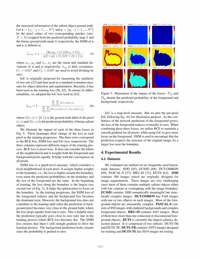
We illustrate the impact of each of the three losses in

Fig. 5. These heatmaps show change of the loss at each

pixel as the training progresses. The three rows correspond

to the BCE loss, SSIM loss and IoU loss, respectively. The

three columns represent different stages of the training pro-

cess. BCE loss is pixel-wise. It does not consider the labels

of the neighborhood and it weights both the foreground and

background pixels equally. It helps with the convergence on

all pixels.

SSIM loss is a patch-level measure, which considers a

local neighborhood of each pixel. It assigns higher weights

to the boundary, i.e., the loss is higher around the boundary,

even when the predicted probabilities on the boundary and

the rest of the foreground are the same. In the beginning

of training, the loss along the boundary is the largest (see

second row of Fig. 5). It helps the optimization to focus on

the boundary. As the training progresses, the SSIM loss of

the foreground reduces and the background loss becomes

the dominant term. However, the background loss does not

contribute to the training until when the prediction of back-

ground pixel becomes very close to the ground truth, where

the loss drops rapidly from one to zero. This is helpful since

the prediction typically goes close to zero only late in the

training process where BCE loss becomes flat. The SSIM

loss ensures that there’s still enough gradient to drive the

learning process. The background prediction looks cleaner

since the probability is pushed to zero.

0

0.5

1

1.5

2

2.5

3

0

0.5

1

1.5

2

2.5

3

0

0.5

1

1.5

2

2.5

3

0

0.5

1

1.5

0

0.5

1

1.5

0

0.5

1

1.5

0

0.1

0.2

0.3

0.4

0.5

0.6

0.7

0.8

0.9

1

0

0.1

0.2

0.3

0.4

0.5

0.6

0.7

0.8

0.9

1

0

0.1

0.2

0.3

0.4

0.5

0.6

0.7

0.8

0.9

1

Figure 5. Illustration of the impact of the losses. Pfg and

Pbg denote the predicted probability of the foreground and

background, respectively.

IoU is a map-level measure. But we plot the per-pixel

IoU following Eq. (6) for illustration purpose. As the con-

fidence of the network prediction of the foreground grows,

the loss of the foreground reduces eventually to zero. When

combining these three losses, we utilize BCE to maintain a

smooth gradient for all pixels, while using IoU to give more

focus on the foreground. SSIM is used to encourage that the

prediction respects the structure of the original image, by a

larger loss near the boundary.

4. Experimental Results

4.1. Datasets

We evaluated our method on six frequently used bench-

mark datasets: SOD [45], ECSSD [68], DUT-OMRON

[69], PASCAL-S [37], HKU-IS [33], DUTS [62]. SOD

contains 300 images which are originally designed for

image segmentation. These images are very challenging

since most of them contains multiple salient objects either

with low contrast or overlapping with the image boundary.

ECSSD contains 1000 semantically meaningful but struc-

turally complex images. DUT-OMRON has 5168 images

with one or two objects in each images. Most of the fore-

ground objects are structurally complex. PASCAL-S con-

sists of 850 images with cluttered backgrounds and complex

foreground objects. HKU-IS contains 4447 images. Most

of them have more than one connected or disconnected fore-

ground objects. DUTS is currently the largest saliency de-

tection dataset. It is comprised of two subsets: DUTS-TR

and DUTS-TE. DUTS-TR contains 10553 images designed

for training and DUTS-TE has 5019 images for testing.

7483

4.2. Implementation and Experimental Setup

We train our network using the DUTS-TR dataset, which

has 10553 images. Before training, the dataset is aug-

mented by horizontal flipping to 21106 images. During

training, each image is first resized to 256×256 and ran-

domly cropped to 224×224. Part of the encoder parame-

ters are initialized from the ResNet-34 model [16]. Other

convolutional layers are initialized by Xavier [10]. We uti-

lize the Adam optimizer [26] to train our network and its

hyper parameters are set to the default values, where the

initial learning rate lr=1e-3, betas=(0.9, 0.999), eps=1e-8,

weight decay=0. We train the network until the loss con-

verges without using validation set. The training loss con-

verges after 400k iterations with a batch size of 8 and the

whole training process takes about 125 hours. During test-

ing, the input image is resized to 256×256 and fed into the

network to obtain its saliency map. Then, the saliency map

(256×256) is resized back to the original size of the input

image. Both the resizing processes use bilinear interpola-

tion.

We implement our network based on the publicly avail-

able framework: Pytorch 0.4.0 [49]. An eight-core PC with

an AMD Ryzen 1800x 3.5 GHz CPU (with 32GB RAM)

and a GTX 1080ti GPU (with 11GB memory) is used for

both training and testing. The inference for a 256×256 im-

age only takes 0.040s (25 fps). The source code will be

released.

4.3. Evaluation Metrics

We use four measures to evaluate our method: Precision-

Recall (PR) curve, F-measure, Mean Absolute Error (MAE)

and relaxed F-measure of boundary (relaxF bβ).

PR curve is a standard way of evaluating the predicted

saliency probability maps. The precision and recall of a

saliency map are computed by comparing the binarized

saliency map against the ground truth mask. Each binariz-

ing threshold results in a pair of average precision and recall

over all saliency maps in a dataset. Varying the threshold

from 0 to 1 produces a sequence of precision-recall pairs,

which is plotted as the PR curve.

Then, to have a comprehensive measure on both preci-

sion and recall, Fβ is computed based on each pair of pre-

cision and recall as:

Fβ = (1+β2)×Precision×Recall

β2×Precision+Recall

(7)

where β2 is set to 0.3 to weight precision more than recall

[1]. The maximum Fβ (maxFβ) of each dataset is reported

in this paper.

MAE [51] denotes the average absolute per-pixel differ-

ence between a predicted saliency map and its ground truth

mask. Given a saliency map, its MAE is defined as:

MAE = 1H×W

∑H

r=1

∑W

c=1|S(r, c)−G(r, c)| (8)

Ablation Configurations maxFβ relaxF bβ MAE

Arc

hit

ectu

re

Baseline U-Net [57] + ℓbce 0.896 0.669 0.066En-De + ℓbce 0.929 0.767 0.047

En-De+Sup + ℓbce 0.934 0.805 0.040En-De+Sup+RRM LC + ℓbce 0.936 0.803 0.040En-De+Sup+RRM MS + ℓbce 0.935 0.804 0.042

En-De+Sup+RRM Ours + ℓbce 0.937 0.806 0.042

Lo

ss

En-De+Sup+RRM Ours + ℓssim 0.924 0.808 0.042En-De+Sup+RRM Ours + ℓiou 0.933 0.795 0.039En-De+Sup+RRM Ours + ℓbs 0.940 0.815 0.040En-De+Sup+RRM Ours + ℓbi 0.940 0.813 0.038En-De+Sup+RRM Ours + ℓbsi 0.942 0.826 0.037

Table 1. Ablation study on different architectures and

losses: En-De: Encoder-Decoder, Sup: side output super-

vision; ℓbi = ℓbce + ℓiou, ℓbs = ℓbce + ℓssim, ℓbsi =ℓbce + ℓssim + ℓiou.

where S and G are saliency probability map and its ground

truth respectively, H and W represents the height and width

of the saliency map and (r, c) denotes the pixel coordi-

nates. For a dataset, its MAE is the average MAE of all

the saliency maps.

Additionally, we adopt the relaxed F-measure relaxF bβ

[7] to quantitatively evaluate boundaries. Given a saliency

map S, we first convert it to a binary mask Sbw using a

threshold of 0.5. Then, we obtain the mask of its one pixel

wide boundary by conducting an XOR(Sbw, Serd) opera-

tion where Serd is the eroded binary mask [14] of Sbw. The

same method is used to get the boundaries of ground truth

mask. The relaxed boundary precision (relaxPrecisionb)

is then defined as the fraction of predicted boundary pix-

els within a range of ρ pixels from ground truth boundary

pixels. The relaxed boundary recall (relaxRecallb) mea-

sures the fraction of ground truth boundary pixels that are

within ρ pixels of predicted boundary pixels. In our experi-

ments, we set the slack parameter ρ to 3 similar to the pre-

vious studies [44, 58, 77]. The relaxed boundary F-measure

relaxF bβ of each predicted saliency map is computed using

equation (7), in which Precision and Recall are replaced

by relaxPrecisionb and relaxRecallb. For each dataset, we

report its average relaxF bβ of all predicted saliency maps.

4.4. Ablation Study

In this section, we validate the effectiveness of each key

components used in our model. The ablation study contains

two parts: architecture ablation and loss ablation. The abla-

tion experiments are conducted on the ECSSD dataset.

Architecture ablation: To prove the effectiveness of our

BASNet, we report the quantitative comparison results of

our model against other related architectures. We take U-

Net [57] as our baseline network. Then we start with our

proposed Encoder-Decoder network and progressively ex-

tend it with densely side output supervision and different

residual refinement modules including RRM LC, RRM MS

7484

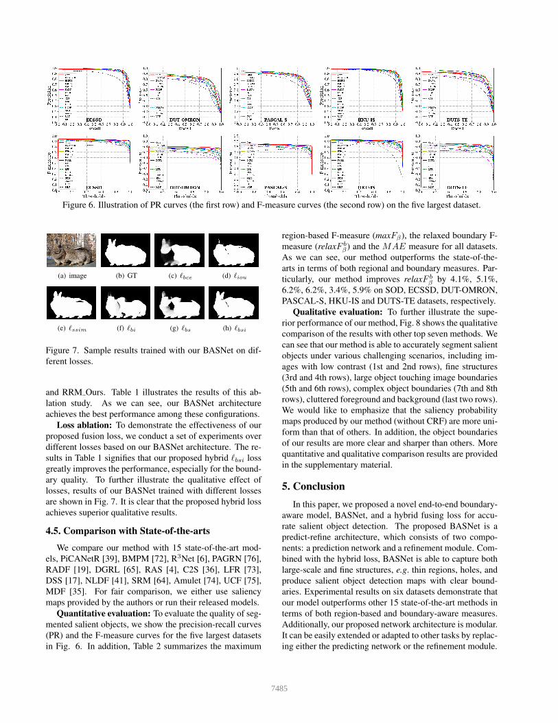
Figure 6. Illustration of PR curves (the first row) and F-measure curves (the second row) on the five largest dataset.

(a) image (b) GT (c) ℓbce (d) ℓiou

(e) ℓssim (f) ℓbi (g) ℓbs (h) ℓbsi

Figure 7. Sample results trained with our BASNet on dif-

ferent losses.

and RRM Ours. Table 1 illustrates the results of this ab-

lation study. As we can see, our BASNet architecture

achieves the best performance among these configurations.

Loss ablation: To demonstrate the effectiveness of our

proposed fusion loss, we conduct a set of experiments over

different losses based on our BASNet architecture. The re-

sults in Table 1 signifies that our proposed hybrid ℓbsi loss

greatly improves the performance, especially for the bound-

ary quality. To further illustrate the qualitative effect of

losses, results of our BASNet trained with different losses

are shown in Fig. 7. It is clear that the proposed hybrid loss

achieves superior qualitative results.

4.5. Comparison with State­of­the­arts

We compare our method with 15 state-of-the-art mod-

els, PiCANetR [39], BMPM [72], R3Net [6], PAGRN [76],

RADF [19], DGRL [65], RAS [4], C2S [36], LFR [73],

DSS [17], NLDF [41], SRM [64], Amulet [74], UCF [75],

MDF [35]. For fair comparison, we either use saliency

maps provided by the authors or run their released models.

Quantitative evaluation: To evaluate the quality of seg-

mented salient objects, we show the precision-recall curves

(PR) and the F-measure curves for the five largest datasets

in Fig. 6. In addition, Table 2 summarizes the maximum

region-based F-measure (maxFβ), the relaxed boundary F-

measure (relaxF bβ) and the MAE measure for all datasets.

As we can see, our method outperforms the state-of-the-

arts in terms of both regional and boundary measures. Par-

ticularly, our method improves relaxF bβ by 4.1%, 5.1%,

6.2%, 6.2%, 3.4%, 5.9% on SOD, ECSSD, DUT-OMRON,

PASCAL-S, HKU-IS and DUTS-TE datasets, respectively.

Qualitative evaluation: To further illustrate the supe-

rior performance of our method, Fig. 8 shows the qualitative

comparison of the results with other top seven methods. We

can see that our method is able to accurately segment salient

objects under various challenging scenarios, including im-

ages with low contrast (1st and 2nd rows), fine structures

(3rd and 4th rows), large object touching image boundaries

(5th and 6th rows), complex object boundaries (7th and 8th

rows), cluttered foreground and background (last two rows).

We would like to emphasize that the saliency probability

maps produced by our method (without CRF) are more uni-

form than that of others. In addition, the object boundaries

of our results are more clear and sharper than others. More

quantitative and qualitative comparison results are provided

in the supplementary material.

5. Conclusion

In this paper, we proposed a novel end-to-end boundary-

aware model, BASNet, and a hybrid fusing loss for accu-

rate salient object detection. The proposed BASNet is a

predict-refine architecture, which consists of two compo-

nents: a prediction network and a refinement module. Com-

bined with the hybrid loss, BASNet is able to capture both

large-scale and fine structures, e.g. thin regions, holes, and

produce salient object detection maps with clear bound-

aries. Experimental results on six datasets demonstrate that

our model outperforms other 15 state-of-the-art methods in

terms of both region-based and boundary-aware measures.

Additionally, our proposed network architecture is modular.

It can be easily extended or adapted to other tasks by replac-

ing either the predicting network or the refinement module.

7485

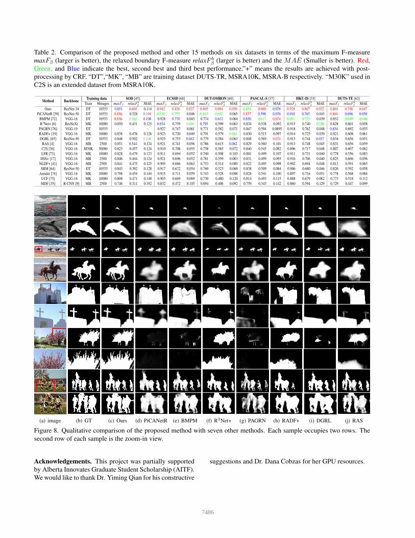
Table 2. Comparison of the proposed method and other 15 methods on six datasets in terms of the maximum F-measure

maxFβ (larger is better), the relaxed boundary F-measure relaxF bβ (larger is better) and the MAE (Smaller is better). Red,

Green, and Blue indicate the best, second best and third best performance.”+” means the results are achieved with post-

processing by CRF. “DT”,“MK”, “MB” are training dataset DUTS-TR, MSRA10K, MSRA-B respectively. “M30K” used in

C2S is an extended dataset from MSRA10K.

Method BackboneTraining data SOD [45] ECSSD [68] DUT-OMRON [69] PASCAL-S [37] HKU-IS [33] DUTS-TE [62]

Train #Images maxFβ relaxF bβ MAE maxFβ relaxF b

β MAE maxFβ relaxF bβ MAE maxFβ relaxF b

β MAE maxFβ relaxF bβ MAE maxFβ relaxF b

β MAE

Ours ResNet-34 DT 10553 0.851 0.603 0.114 0.942 0.826 0.037 0.805 0.694 0.056 0.854 0.660 0.076 0.928 0.807 0.032 0.860 0.758 0.047

PiCANetR [39] ResNet-50 DT 10553 0.856 0.528 0.104 0.935 0.775 0.046 0.803 0.632 0.065 0.857 0.598 0.076 0.918 0.765 0.043 0.860 0.696 0.050

BMPM [72] VGG-16 DT 10553 0.856 0.562 0.108 0.928 0.770 0.045 0.774 0.612 0.064 0.850 0.617 0.074 0.921 0.773 0.039 0.852 0.699 0.048

R3Net+ [6] ResNeXt MK 10000 0.850 0.431 0.125 0.934 0.759 0.040 0.795 0.599 0.063 0.834 0.538 0.092 0.915 0.740 0.036 0.828 0.601 0.058

PAGRN [76] VGG-19 DT 10553 - - - 0.927 0.747 0.061 0.771 0.582 0.071 0.847 0.594 0.0895 0.918 0.762 0.048 0.854 0.692 0.055

RADF+ [19] VGG-16 MK 10000 0.838 0.476 0.126 0.923 0.720 0.049 0.791 0.579 0.061 0.830 0.515 0.097 0.914 0.725 0.039 0.821 0.608 0.061

DGRL [65] ResNet-50 DT 10553 0.848 0.502 0.106 0.925 0.753 0.042 0.779 0.584 0.063 0.848 0.569 0.074 0.913 0.744 0.037 0.834 0.656 0.051

RAS [4] VGG-16 MB 2500 0.851 0.544 0.124 0.921 0.741 0.056 0.786 0.615 0.062 0.829 0.560 0.101 0.913 0.748 0.045 0.831 0.656 0.059

C2S [36] VGG-16 M30K 30000 0.823 0.457 0.124 0.910 0.708 0.055 0.758 0.565 0.072 0.840 0.543 0.082 0.896 0.717 0.048 0.807 0.607 0.062

LFR [73] VGG-16 MK 10000 0.828 0.479 0.123 0.911 0.694 0.052 0.740 0.508 0.103 0.801 0.499 0.107 0.911 0.731 0.040 0.778 0.556 0.083

DSS+ [17] VGG-16 MB 2500 0.846 0.444 0.124 0.921 0.696 0.052 0.781 0.559 0.063 0.831 0.499 0.093 0.916 0.706 0.040 0.825 0.606 0.056

NLDF+ [41] VGG-16 MB 2500 0.841 0.475 0.125 0.905 0.666 0.063 0.753 0.514 0.080 0.822 0.495 0.098 0.902 0.694 0.048 0.813 0.591 0.065

SRM [64] ResNet-50 DT 10553 0.843 0.392 0.128 0.917 0.672 0.054 0.769 0.523 0.069 0.838 0.509 0.084 0.906 0.680 0.046 0.826 0.592 0.058

Amulet [74] VGG-16 MK 10000 0.798 0.454 0.144 0.915 0.711 0.059 0.743 0.528 0.098 0.828 0.541 0.100 0.897 0.716 0.051 0.778 0.568 0.084

UCF [75] VGG-16 MK 10000 0.808 0.471 0.148 0.903 0.669 0.069 0.730 0.480 0.120 0.814 0.493 0.115 0.888 0.679 0.062 0.773 0.518 0.112

MDF [35] R-CNN [9] MB 2500 0.746 0.311 0.192 0.832 0.472 0.105 0.694 0.406 0.092 0.759 0.343 0.142 0.860 0.594 0.129 0.729 0.447 0.099

(a) image (b) GT (c) Ours (d) PiCANetR (e) BMPM (f) R3Net+ (g) PAGRN (h) RADF+ (i) DGRL (j) RAS

Figure 8. Qualitative comparison of the proposed method with seven other methods. Each sample occupies two rows. The

second row of each sample is the zoom-in view.

Acknowledgements. This project was partially supported

by Alberta Innovates Graduate Student Scholarship (AITF).

We would like to thank Dr. Yiming Qian for his constructive

suggestions and Dr. Dana Cobzas for her GPU resources.

7486

References

[1] Radhakrishna Achanta, Sheila Hemami, Francisco Estrada,

and Sabine Susstrunk. Frequency-tuned salient region detec-

tion. In Computer vision and pattern recognition, 2009. cvpr

2009. ieee conference on, pages 1597–1604. IEEE, 2009.

[2] Vijay Badrinarayanan, Alex Kendall, and Roberto Cipolla.

Segnet: A deep convolutional encoder-decoder architecture

for image segmentation. IEEE Transactions on Pattern Anal-

ysis & Machine Intelligence, (12):2481–2495, 2017.

[3] Ali Borji, Ming-Ming Cheng, Huaizu Jiang, and Jia Li.

Salient object detection: A benchmark. IEEE Trans. Image

Processing, 24(12):5706–5722, 2015.

[4] Shuhan Chen, Xiuli Tan, Ben Wang, and Xuelong Hu. Re-

verse attention for salient object detection. In Computer

Vision - ECCV 2018 - 15th European Conference, Mu-

nich, Germany, September 8-14, 2018, Proceedings, Part IX,

pages 236–252, 2018.

[5] Pieter-Tjerk de Boer, Dirk P. Kroese, Shie Mannor, and

Reuven Y. Rubinstein. A tutorial on the cross-entropy

method. Annals OR, 134(1):19–67, 2005.

[6] Zijun Deng, Xiaowei Hu, Lei Zhu, Xuemiao Xu, Jing Qin,

Guoqiang Han, and Pheng-Ann Heng. R3net: Recurrent

residual refinement network for saliency detection. IJCAI,

2018.

[7] Marc Ehrig and Jerome Euzenat. Relaxed precision and re-

call for ontology matching. In Proc. K-Cap 2005 workshop

on Integrating ontology, pages 25–32. No commercial edi-

tor., 2005.

[8] Lucas Fidon, Wenqi Li, Luis C. Herrera, Jinendra

Ekanayake, Neil Kitchen, Sebastien Ourselin, and Tom Ver-

cauteren. Generalised wasserstein dice score for imbalanced

multi-class segmentation using holistic convolutional net-

works. In Brainlesion: Glioma, Multiple Sclerosis, Stroke

and Traumatic Brain Injuries - Third International Work-

shop, BrainLes 2017, Held in Conjunction with MICCAI

2017, Quebec City, QC, Canada, pages 64–76, 2017.

[9] Ross Girshick, Jeff Donahue, Trevor Darrell, and Jitendra

Malik. Rich feature hierarchies for accurate object detection

and semantic segmentation. In Proceedings of the IEEE con-

ference on computer vision and pattern recognition, pages

580–587, 2014.

[10] Xavier Glorot and Yoshua Bengio. Understanding the diffi-

culty of training deep feedforward neural networks. In Pro-

ceedings of the Thirteenth International Conference on Ar-

tificial Intelligence and Statistics, AISTATS 2010, Chia La-

guna Resort, Sardinia, Italy, May 13-15, 2010, pages 249–

256, 2010.

[11] Stas Goferman, Lihi Zelnik-Manor, and Ayellet Tal.

Context-aware saliency detection. IEEE transactions on pat-

tern analysis and machine intelligence, 34(10):1915–1926,

2012.

[12] Prakhar Gupta, Shubh Gupta, Ajaykrishnan Jayagopal,

Sourav Pal, and Ritwik Sinha. Saliency prediction for mobile

user interfaces. In 2018 IEEE Winter Conference on Appli-

cations of Computer Vision, WACV 2018, Lake Tahoe, NV,

USA, March 12-15, 2018, pages 1529–1538, 2018.

[13] Richard HR Hahnloser and H Sebastian Seung. Permit-

ted and forbidden sets in symmetric threshold-linear net-

works. In Advances in Neural Information Processing Sys-

tems, pages 217–223, 2001.

[14] Robert M Haralick, Stanley R Sternberg, and Xinhua

Zhuang. Image analysis using mathematical morphology.

IEEE transactions on pattern analysis and machine intelli-

gence, (4):532–550, 1987.

[15] Kaiming He, Xiangyu Zhang, Shaoqing Ren, and Jian Sun.

Spatial pyramid pooling in deep convolutional networks for

visual recognition. In European conference on computer vi-

sion, pages 346–361. Springer, 2014.

[16] Kaiming He, Xiangyu Zhang, Shaoqing Ren, and Jian Sun.

Deep residual learning for image recognition. In Proceed-

ings of the IEEE conference on computer vision and pattern

recognition, pages 770–778, 2016.

[17] Qibin Hou, Ming-Ming Cheng, Xiaowei Hu, Ali Borji,

Zhuowen Tu, and Philip Torr. Deeply supervised salient ob-

ject detection with short connections. In 2017 IEEE Confer-

ence on Computer Vision and Pattern Recognition (CVPR),

pages 5300–5309. IEEE, 2017.

[18] Ping Hu, Bing Shuai, Jun Liu, and Gang Wang. Deep level

sets for salient object detection. In CVPR, volume 1, page 2,

2017.

[19] Xiaowei Hu, Lei Zhu, Jing Qin, Chi-Wing Fu, and Pheng-

Ann Heng. Recurrently aggregating deep features for salient

object detection. In Proceedings of AAAI-18, New Orleans,

Louisiana, USA, pages 6943–6950, 2018.

[20] Xun Huang, Chengyao Shen, Xavier Boix, and Qi Zhao. Sal-

icon: Reducing the semantic gap in saliency prediction by

adapting deep neural networks. In Proceedings of the IEEE

International Conference on Computer Vision, pages 262–

270, 2015.

[21] Sergey Ioffe and Christian Szegedy. Batch normalization:

Accelerating deep network training by reducing internal co-

variate shift. arXiv preprint arXiv:1502.03167, 2015.

[22] Md Amirul Islam, Mahmoud Kalash, Mrigank Rochan,

Neil DB Bruce, and Yang Wang. Salient object detection

using a context-aware refinement network.

[23] Paul Jaccard. The distribution of the flora in the alpine zone.

1. New phytologist, 11(2):37–50, 1912.

[24] Martin Jagersand. Saliency maps and attention selection in

scale and spatial coordinates: An information theoretic ap-

proach. In ICCV, pages 195–202, 1995.

[25] Timor Kadir and Michael Brady. Saliency, scale and im-

age description. International Journal of Computer Vision,

45(2):83–105, 2001.

[26] Diederik P Kingma and Jimmy Ba. Adam: A method for

stochastic optimization. arXiv preprint arXiv:1412.6980,

2014.

[27] Philipp Krahenbuhl and Vladlen Koltun. Efficient inference

in fully connected crfs with gaussian edge potentials. In Ad-

vances in neural information processing systems, pages 109–

117, 2011.

[28] Alex Krizhevsky, Ilya Sutskever, and Geoffrey E. Hinton.

Imagenet classification with deep convolutional neural net-

works. In Advances in Neural Information Processing Sys-

tems 25: 26th Annual Conference on Neural Information

7487

Processing Systems 2012. Proceedings of a meeting held De-

cember 3-6, 2012, Lake Tahoe, Nevada, United States., pages

1106–1114, 2012.

[29] Srinivas SS Kruthiventi, Vennela Gudisa, Jaley H Dholakiya,

and R Venkatesh Babu. Saliency unified: A deep architec-

ture for simultaneous eye fixation prediction and salient ob-

ject segmentation. In Proceedings of the IEEE Conference

on Computer Vision and Pattern Recognition, pages 5781–

5790, 2016.

[30] Jason Kuen, Zhenhua Wang, and Gang Wang. Recurrent at-

tentional networks for saliency detection. In Proceedings

of the IEEE Conference on Computer Vision and Pattern

Recognition, pages 3668–3677, 2016.

[31] Chen-Yu Lee, Saining Xie, Patrick Gallagher, Zhengyou

Zhang, and Zhuowen Tu. Deeply-supervised nets. In Ar-

tificial Intelligence and Statistics, pages 562–570, 2015.

[32] Hyemin Lee and Daijin Kim. Salient region-based online

object tracking. In 2018 IEEE Winter Conference on Appli-

cations of Computer Vision, WACV 2018, Lake Tahoe, NV,

USA, March 12-15, 2018, pages 1170–1177, 2018.

[33] Guanbin Li and Yizhou Yu. Visual saliency based on multi-

scale deep features. In Proceedings of the IEEE conference

on computer vision and pattern recognition, pages 5455–

5463, 2015.

[34] Guanbin Li and Yizhou Yu. Deep contrast learning for salient

object detection. In Proceedings of the IEEE Conference on

Computer Vision and Pattern Recognition, pages 478–487,

2016.

[35] Guanbin Li and Yizhou Yu. Visual saliency detection based

on multiscale deep cnn features. IEEE Transactions on Im-

age Processing, 25(11):5012–5024, 2016.

[36] Xin Li, Fan Yang, Hong Cheng, Wei Liu, and Dinggang

Shen. Contour knowledge transfer for salient object detec-

tion. In Computer Vision - ECCV 2018 - 15th European Con-

ference, Munich, Germany, September 8-14, 2018, Proceed-

ings, Part XV, pages 370–385, 2018.

[37] Yin Li, Xiaodi Hou, Christof Koch, James M Rehg, and

Alan L Yuille. The secrets of salient object segmentation.

In Proceedings of the IEEE Conference on Computer Vision

and Pattern Recognition, pages 280–287, 2014.

[38] Nian Liu and Junwei Han. Dhsnet: Deep hierarchical

saliency network for salient object detection. In 2016 IEEE

Conference on Computer Vision and Pattern Recognition

(CVPR), pages 678–686, 2016.

[39] Nian Liu, Junwei Han, and Ming-Hsuan Yang. Picanet:

Learning pixel-wise contextual attention for saliency detec-

tion. In Proceedings of the IEEE Conference on Computer

Vision and Pattern Recognition, pages 3089–3098, 2018.

[40] Nian Liu, Junwei Han, Dingwen Zhang, Shifeng Wen, and

Tianming Liu. Predicting eye fixations using convolutional

neural networks. In Proceedings of the IEEE Conference on

Computer Vision and Pattern Recognition, pages 362–370,

2015.

[41] Zhiming Luo, Akshaya Mishra, Andrew Achkar, Justin

Eichel, Shaozi Li, and Pierre-Marc Jodoin. Non-local deep

features for salient object detection. In Computer Vision

and Pattern Recognition (CVPR), 2017 IEEE Conference on,

pages 6593–6601. IEEE, 2017.

[42] Gellert Mattyus, Wenjie Luo, and Raquel Urtasun. Deep-

roadmapper: Extracting road topology from aerial images.

[43] Roey Mechrez, Eli Shechtman, and Lihi Zelnik-Manor.

Saliency driven image manipulation. In 2018 IEEE Win-

ter Conference on Applications of Computer Vision, WACV

2018, Lake Tahoe, NV, USA, March 12-15, 2018, pages

1368–1376, 2018.

[44] Volodymyr Mnih and Geoffrey E Hinton. Learning to detect

roads in high-resolution aerial images. In European Confer-

ence on Computer Vision, pages 210–223. Springer, 2010.

[45] Vida Movahedi and James H Elder. Design and percep-

tual validation of performance measures for salient object

segmentation. In Computer Vision and Pattern Recognition

Workshops (CVPRW), 2010 IEEE Computer Society Confer-

ence on, pages 49–56. IEEE, 2010.

[46] David Mumford and Jayant Shah. Optimal approximations

by piecewise smooth functions and associated variational

problems. Communications on pure and applied mathemat-

ics, 42(5):577–685, 1989.

[47] Gattigorla Nagendar, Digvijay Singh, Vineeth N. Balasub-

ramanian, and C. V. Jawahar. Neuro-iou: Learning a sur-

rogate loss for semantic segmentation. In British Machine

Vision Conference 2018, BMVC 2018, Northumbria Univer-

sity, Newcastle, UK, September 3-6, 2018, page 278, 2018.

[48] Stanley Osher and James A Sethian. Fronts propagating with

curvature-dependent speed: algorithms based on hamilton-

jacobi formulations. Journal of computational physics,

79(1):12–49, 1988.

[49] Adam Paszke, Sam Gross, Soumith Chintala, Gregory

Chanan, Edward Yang, Zachary DeVito, Zeming Lin, Al-

ban Desmaison, Luca Antiga, and Adam Lerer. Automatic

differentiation in pytorch. In NIPS-W, 2017.

[50] Chao Peng, Xiangyu Zhang, Gang Yu, Guiming Luo, and

Jian Sun. Large kernel mattersimprove semantic segmen-

tation by global convolutional network. In Computer Vision

and Pattern Recognition (CVPR), 2017 IEEE Conference on,

pages 1743–1751. IEEE, 2017.

[51] Federico Perazzi, Philipp Krahenbuhl, Yael Pritch, and

Alexander Hornung. Saliency filters: Contrast based filtering

for salient region detection. In Computer Vision and Pattern

Recognition (CVPR), 2012 IEEE Conference on, pages 733–

740. IEEE, 2012.

[52] Xuebin Qin, Shida He, Camilo Perez Quintero, Abhineet

Singh, Masood Dehghan, and Martin Jagersand. Real-time

salient closed boundary tracking via line segments percep-

tual grouping. In 2017 IEEE/RSJ International Conference

on Intelligent Robots and Systems, IROS 2017, Vancouver,

BC, Canada, September 24-28, 2017, pages 4284–4289,

2017.

[53] Xuebin Qin, Shida He, Xiucheng Yang, Masood Dehghan,

Qiming Qin, and Martin Jagersand. Accurate outline extrac-

tion of individual building from very high-resolution opti-

cal images. IEEE Geoscience and Remote Sensing Letters,

(99):1–5, 2018.

[54] Xuebin Qin, Shida He, Zichen Zhang, Masood Dehghan,

and Martin Jagersand. Bylabel: A boundary based semi-

automatic image annotation tool. In 2018 IEEE Winter Con-

7488

ference on Applications of Computer Vision (WACV), pages

1804–1813. IEEE, 2018.

[55] Xuebin Qin, Shida He, Zichen Vincent Zhang, Masood

Dehghan, and Martin Jagersand. Real-time salient closed

boundary tracking using perceptual grouping and shape pri-

ors. In British Machine Vision Conference 2017, BMVC

2017, London, UK, September 4-7, 2017, 2017.

[56] Md Atiqur Rahman and Yang Wang. Optimizing

intersection-over-union in deep neural networks for image

segmentation. In International Symposium on Visual Com-

puting, pages 234–244. Springer, 2016.

[57] Olaf Ronneberger, Philipp Fischer, and Thomas Brox. U-

net: Convolutional networks for biomedical image segmen-

tation. In International Conference on Medical image com-

puting and computer-assisted intervention, pages 234–241.

Springer, 2015.

[58] Shunta Saito, Takayoshi Yamashita, and Yoshimitsu Aoki.

Multiple object extraction from aerial imagery with convo-

lutional neural networks. Electronic Imaging, 2016(10):1–9,

2016.

[59] Karen Simonyan and Andrew Zisserman. Very deep convo-

lutional networks for large-scale image recognition. arXiv

preprint arXiv:1409.1556, 2014.

[60] R Sai Srivatsa and R Venkatesh Babu. Salient object detec-

tion via objectness measure. In Image Processing (ICIP),

2015 IEEE International Conference on, pages 4481–4485.

IEEE, 2015.

[61] Lijun Wang, Huchuan Lu, Xiang Ruan, and Ming-Hsuan

Yang. Deep networks for saliency detection via local esti-

mation and global search. In Proceedings of the IEEE Con-

ference on Computer Vision and Pattern Recognition, pages

3183–3192, 2015.

[62] Lijun Wang, Huchuan Lu, Yifan Wang, Mengyang Feng,

Dong Wang, Baocai Yin, and Xiang Ruan. Learning to de-

tect salient objects with image-level supervision. In Proc.

IEEE Conf. Comput. Vis. Pattern Recognit.(CVPR), pages

136–145, 2017.

[63] Linzhao Wang, Lijun Wang, Huchuan Lu, Pingping Zhang,

and Xiang Ruan. Salient object detection with recurrent fully

convolutional networks. IEEE Transactions on Pattern Anal-

ysis and Machine Intelligence, 2018.

[64] Tiantian Wang, Ali Borji, Lihe Zhang, Pingping Zhang, and

Huchuan Lu. A stagewise refinement model for detecting

salient objects in images. In IEEE International Conference

on Computer Vision, ICCV 2017, Venice, Italy, October 22-

29, 2017, pages 4039–4048, 2017.

[65] Tiantian Wang, Lihe Zhang, Shuo Wang, Huchuan Lu, Gang

Yang, Xiang Ruan, and Ali Borji. Detect globally, refine

locally: A novel approach to saliency detection. In Proceed-

ings of the IEEE Conference on Computer Vision and Pattern

Recognition, pages 3127–3135, 2018.

[66] Zhou Wang, Eero P Simoncelli, and Alan C Bovik. Multi-

scale structural similarity for image quality assessment. In

The Thrity-Seventh Asilomar Conference on Signals, Sys-

tems & Computers, 2003, volume 2, pages 1398–1402. Ieee,

2003.

[67] Saining Xie and Zhuowen Tu. Holistically-nested edge de-

tection. In Proceedings of the IEEE international conference

on computer vision, pages 1395–1403, 2015.

[68] Qiong Yan, Li Xu, Jianping Shi, and Jiaya Jia. Hierarchical

saliency detection. In Proceedings of the IEEE Conference

on Computer Vision and Pattern Recognition, pages 1155–

1162, 2013.

[69] Chuan Yang, Lihe Zhang, Huchuan Lu, Xiang Ruan, and

Ming-Hsuan Yang. Saliency detection via graph-based man-

ifold ranking. In Proceedings of the IEEE conference on

computer vision and pattern recognition, pages 3166–3173,

2013.

[70] Fisher Yu and Vladlen Koltun. Multi-scale context

aggregation by dilated convolutions. arXiv preprint

arXiv:1511.07122, 2015.

[71] Jianming Zhang, Stan Sclaroff, Zhe Lin, Xiaohui Shen,

Brian Price, and Radomir Mech. Minimum barrier salient

object detection at 80 fps. In Proceedings of the IEEE inter-

national conference on computer vision, pages 1404–1412,

2015.

[72] Lu Zhang, Ju Dai, Huchuan Lu, You He, and Gang Wang. A

bi-directional message passing model for salient object de-

tection. In Proceedings of the IEEE Conference on Computer

Vision and Pattern Recognition, pages 1741–1750, 2018.

[73] Pingping Zhang, Wei Liu, Huchuan Lu, and Chunhua Shen.

Salient object detection by lossless feature reflection. In Pro-

ceedings of the Twenty-Seventh International Joint Confer-

ence on Artificial Intelligence, IJCAI 2018, July 13-19, 2018,

Stockholm, Sweden., pages 1149–1155, 2018.

[74] Pingping Zhang, Dong Wang, Huchuan Lu, Hongyu Wang,

and Xiang Ruan. Amulet: Aggregating multi-level convolu-

tional features for salient object detection. In IEEE Interna-

tional Conference on Computer Vision, ICCV 2017, Venice,

Italy, October 22-29, 2017, pages 202–211, 2017.

[75] Pingping Zhang, Dong Wang, Huchuan Lu, Hongyu Wang,

and Baocai Yin. Learning uncertain convolutional features

for accurate saliency detection. In IEEE International Con-

ference on Computer Vision, ICCV 2017, Venice, Italy, Oc-

tober 22-29, 2017, pages 212–221, 2017.

[76] Xiaoning Zhang, Tiantian Wang, Jinqing Qi, Huchuan Lu,

and Gang Wang. Progressive attention guided recurrent net-

work for salient object detection. In Proceedings of the IEEE

Conference on Computer Vision and Pattern Recognition,

pages 714–722, 2018.

[77] Zhengxin Zhang, Qingjie Liu, and Yunhong Wang. Road

extraction by deep residual u-net. IEEE Geoscience and Re-

mote Sensing Letters, 2018.

[78] Kai Zhao, Shanghua Gao, Qibin Hou, Dandan Li, and Ming-

Ming Cheng. Optimizing the f-measure for threshold-free

salient object detection. CoRR, abs/1805.07567, 2018.

[79] Rui Zhao, Wanli Ouyang, Hongsheng Li, and Xiaogang

Wang. Saliency detection by multi-context deep learning.

In Proceedings of the IEEE Conference on Computer Vision

and Pattern Recognition, pages 1265–1274, 2015.

[80] Wangjiang Zhu, Shuang Liang, Yichen Wei, and Jian Sun.

Saliency optimization from robust background detection. In

Proceedings of the IEEE conference on computer vision and

pattern recognition, pages 2814–2821, 2014.

7489