bassline generation agent based on knowledge and …
TRANSCRIPT
BASSLINE GENERATION AGENT BASED ON
KNOWLEDGE AND CONTEXT
Calopa Piedra, Pere
Curs 2014-2015
Directors: Sergi Jordà, Perfecto Herrera, Daniel Gómez
GRAU EN ENGINYERIA EN SISTEMES AUDIOVISUALS
Treball de Fi de Grau
GRAU EN ENGINYERIA EN
xxxxxxxxxxxx

BASSLINE GENERATION AGENT BASED ON
KNOWLEDGE AND CONTEXT
Pere Calopa Piedra
TREBALL FI DE GRAU
Grau en Enginyeria de Sistemes Audiovisuals
ESCOLA SUPERIOR POLITÈCNICA UPF
2015
DIRECTORS DEL TREBALL
Dr. Sergi Jordà, Dr. Perfecto Herrera, Daniel Gòmez
Para ver esta película, debedisponer de QuickTime™ y de
un descompresor .

ii

iii
Aquest projecte està dedicat a tots aquells que senten passió per la música i la
tecnologia.


v
Agraïments
Agraeixo especialment als meus tutors la gran ajuda que m’han ofert en la realització
d’aquest projecte. Més enllá del la part docent, valoro d’una manera molt positiva la
implicació en el projecte.
També dóno les gràcies a Julio Navas i a tots el voluntaris per participar en el
desenvolupament d’aquest projecte.


vii
Abstract The main goal of this project is to develop a musical agent system that generates basslines
from a certain style/genre of music. The project combines an automatic generation process
with some user interaction. The automatic generation process is based on knowledge
extracted from available data (i.e., MIDI files) and real-time adaptation to music context.
Input data consists of a collection bassline loops that are referred to a certain style/genre,
so the individual loops must have a relation between them .The system analyzes the
collection to extract useful information to model some of the genre conventions with
relation to the rhythmic patterning. The knowledge extracted is used to generate basslines
that belong to the style/genre of interest, allowing the user to interact with them.
Resum El objectiu principal d’aquest projecte és desenvolupar un agent musical capç de generar
línies de baixos d’un cert estil o génere musical. El projecte combina técniques de generació
automàtica i interacció per part de l’usuari. El procés de generació autmàtica està basat en
el coneixement extret de dades (arxius MIDI) i adaptació en temps real al context musical.
Les dades consisteixen en una colleccío de línies de baixos previament agrupades segons un
estil o gènere musical, aixó asegura que les línies de baix tindran alguna relació entre elles.
El sistema analitza la col·lecció per extreure informació rellevant que permeti model la
col·leció utilitzant patrons rítmics. El coneixement extret s’utilitza per a generar línies de
baixos que pertanyen a un cert estil musical d’interès, permetent a l’usuari interactuar en la
generació.


ix
Prologue
¿How become a sound music?¿What is music?¿Where it comes from?¿Why there is ‘good’
and ‘bad’ music?¿Can it be described?... Trials along history to define music are based on
the hard work of solving the previous questions.
An isolated sound is a natural event, such as a thunder, a dog bark, a footstep…but is not
music till it is listened in context with other sounds. Human sound perception is a
subjective experience. A bird singing is a strictly natural effect, that can also be an
harmonic element with a distinguible timbre.
While a subject can perceive a sound or group of sounds as ‘noise’ another can perceive the
same as a musical piece. Musical events are ephemeral, that spreaded in time conform a
musical piece. In a classical point of view, music is a group of sounds in a determined
order. Along history, different civilizations and cultures,even the most ancient,
experimented with music and attributed to it many interpretations. The common fact is
that music has always been related to emotions,culture and spirit.
There are evidences of the existence of music already in the prehistory, based on the
percussion elements and arcaic trumpets and flutes found during this period. Pitagorics,
active since the VI a.C. , studied arithmetics and music as a same subject, and developed
acoustic and musical models. In many lenguages around the world ‘sing’ and ‘dance’ have
the same word, that is because they consider that singing involves a corporal move. Music
has a very important component of cultural influence. A subject need to belong to a certain
culture to be able to percieve music. Musician along history proposed different notations
and arbitrary statements in order to make possible to read and write music.
The previous examples show how music involves many research areas to understand it,
from antropology to neuropsychology. This project will be focused on research areas such
as music perception, cognition and computation. Those research areas and others related
conform the multidisciplinary science of Music Information Retrieval (MIR).
A first approach of a bassline analisys and generation algorithm will be proposed. This first
aproach is based on recent studies (Cao, 2014) that use perceptual correlated techniques to
group rhythmic patterns in families combined with syncopation computation [3] to
conform a probabilistic model. This studies take in account the concept of meter and
syncopation to group rhythms by its perceptive similitude.


xi
Index
Pàg.
Abstract.......................................................................... vii
Prologue......................................................................... ix
1. SOUND AND MUSIC PERCEPTION AND
DESCRIPTION .............................................................
1
1.1 Musical descriptive atributes .................................. 1
1.2 Music Information Retrieval ................................... 3
1.3 Rhythm and meter.................................................... 4
a) Rhythmic units .......................................................... 4
b) Metrical structures .................................................... 5
c) Time signatures and genres ....................................... 5
1.4 The bass in electronic dance music ......................... 6
a) House Music ............................................................. 7
b) Techno ...................................................................... 7
2. MUSIC RHYTHM FAMILIES THEORY ............... 9
2.1. Syncopation level.................................................... 9
2.2 Rhythmic families ................................................... 10
3. METHOD .................................................................. 11
3.1 Data-set selection .................................................... 11
a) Deep-house data-set .................................................. 12
b) Techno data-set ......................................................... 12
c) Tech-house data-set .................................................. 13
3.2 Custiomizing rhythmic families theory .................. 13
3.3 Method tools ........................................................... 18
3.4 First approach: ‘blind’ analysis .............................. 18
a) Pseudocode ............................................................... 20
3.5 Second approach: binomial model .......................... 21
a) Pseudocode ............................................................... 22
3.6 Genration control parameters .................................. 23
3.7 Results ..................................................................... 23
a) Families distribution ................................................. 24
b) First approach results: ‘blind’ analysis/generation ... 27
c) Second approach results: binomial model ................ 34
4.EVALUATION .......................................................... 39
4.1 Deep-House scoring experiment ............................. 39
a) Participants ................................................................ 39
b) Design........................................................................ 39
c) Materials ................................................................... 41
d) Procedure .................................................................. 42
e) Results ....................................................................... 43
5.NEXT STEPS............................................................. 46
References.................................................................... 49

1
1. SOUND AND MUSIC PERCEPTION AND DESCRIPTION
1.1 Musical descriptive atributes
To achieve the ambitious goal of this project it is necessary to be able to model a certain
genre/style of music. Discriminate which genre belong a certain piece of music is a whole
research area. In this project it is assumed that the musical pieces to be modelized are
previously classified using human genre/style classification. Before looking for what makes
different two pieces of music, focus need to be set on ‘what’ makes those pieces be Music.
¿What have in common Bach, John Cage, Rolling Stones and Aphex Twin?¿Which is the
difference between Bob Marley’s <Redemption Song> and what we can listen in Boqueria
market in Barcelona? The famous composer Edgard Varèse defined music as “Music is
organized sound”. Music is a perceptive phenomenon that ‘happens’ in our brain and is
percieved in multiple atributes and ‘dimensions’. From a mathematichal point of view it is
a great advantage.
The basic percieved elements on any sound are: intensity, pitch, rhythm, duration, tempo,
timbre, pitch contour, spatial position and reverberation. Brain organizes this perceptual
basic atributes into high level concepts like meter, tonality, harmony or melody.
Intensity is the perceptive correlation with the physical amplitude of the sound. This
correlation has a non-linear behaviour and it is still an open research in the
psychoacoustic area.
We assume pitch as the percieved value of a tone. The tone is related directly to the
frequency of the oscilating wave that produce the source of sound, measured in Hertz
(Hz). The pitch value allows us to differentiate two notes and discriminate between
low and high pitches.
Human ear, in average, is able to listen from 20 Hz to 20 KHz. Musical notes are
arbitrary names given to certain tones.
Rhythm can be define as a repeated series of events along time. Particulary, music
rhythm is the frequency at which the music articulations are produced. It also refers to
the duration of a serie of notes and how they are grouped in units.
Tempo refers to the global rhythm of the musical piece. It is measures in beats per
second. Musical time units will be explained in the following chapter.

2
Timbre, is the property of sound that makes different two sounds with the same pitch
and intensity. It is related to the harmonic and spectral features of the emitting sound
source. It gives information about the global color of the sound source, for instance,
we can easily distinguish a piano sound from a trumpet sound. The Acoustical Society
of America defined it as ‘everything related with a sound that is not intensity nor
pitch’.
Pitch countour gives the global envelope that follows a certain melody, taking on
account if a note is lower or higher than the prevoius one.
Spatial position gives information about where the sound comes from. For that
porpose our brain take advantage of our stereo auditive sense.
Reverberation refers to the perception of how far the sound comes from, in
combination with the size and architecture of the listening place.
All this atributes are independent between them, so one atribute can be changed without
altering the other atributes. That means this atributes can be seen as dimensions and can be
scientifically studied independently. The way how this basic percieved elements are
combined, is the main difference between a musical piece and the sound scene in a
crowded market. When this elements are combined with a significance, become music, it is
the origin of high level concepts as meter, tonality, melody and harmony.
Meter is created by the listener subject extracting information about rhythmic patterns
and volume, and how the sound events are grouped between them along time.
Different time signatures used in contemporary music refer to the possible meters that
can be induced in the listener. This topic will be further discussed in next chapters.
Tonality is the hierarchy of importance of the tones used in a musical piece. Its is not a
natural phenomenon but is consequence of the listener experience with a certain kind
of music , musical lenguages knowledge and mental schemes to understand music.

3
Melody is the most prominent theme in a musical piece, the part that you can sing and
our brain is able to extract. The concept of melody can slighty be different depending
in music genres. Rock music tends to use different melodies for different parts of the
song like the verses or chorus. In classical music, the melody works like the starting
basic idea around which the music piece evolves and variate. In contemporary genres
like Techno, melody can be a very basic and monotonous idea evolving through the
music piece.
Harmony is based on how the pitch of the different elements in a musical piece are
related between them. The different combinations of picthes are able to induce
different emotions in the listener like expectation, melancholy and even fear.
1.2 Music Information Retrieval
Music Infomation Retrieval (MIR)[9] is multdisciplinary growing research area that is based
on categorize, manipulate and even create music. Those researches involved in MIR may
have a background in musicology, psychology, academic music study, signal
processing, machine learning or some combination of these. Some exmaples of MIR
research areas are the following: recommender systems, instrument recognition and
separation, music generation and automatic music transcription among other. Some of the
methods used in MIR are the following:
- Data source: MIDI music, metadata, Digital Audio formats, among others
- Feature representation: Features like key,rhythm,chords are analyzed to be applied
in machine learning methods
- Statistics and machine learning: Musical features extraction algorithms are designed
in order to solve problems like: similarity and pattern matching, automatic
transcription, agent systems and many others [9]
4
1.3 Rhythm and meter In this chapter will be covered the musical dimension of rhythm, how it is percieved by
listeners, it’s musical notation and discuss how it is used in different genres.
Rhythm is mostly layered up with a melody, changes of pitch and intensity. Striping down
this elements, leave rhythm as a pure binary sequence of events, a note is played or not.
From a mathematical point of view this is a great advantage so it is possible to transcribe
any rhytmic structure as a sequence of 1’s or 0’s for instance. For this transcription is
necessary to use arbitrary rhythmic units and the concept of time signature.
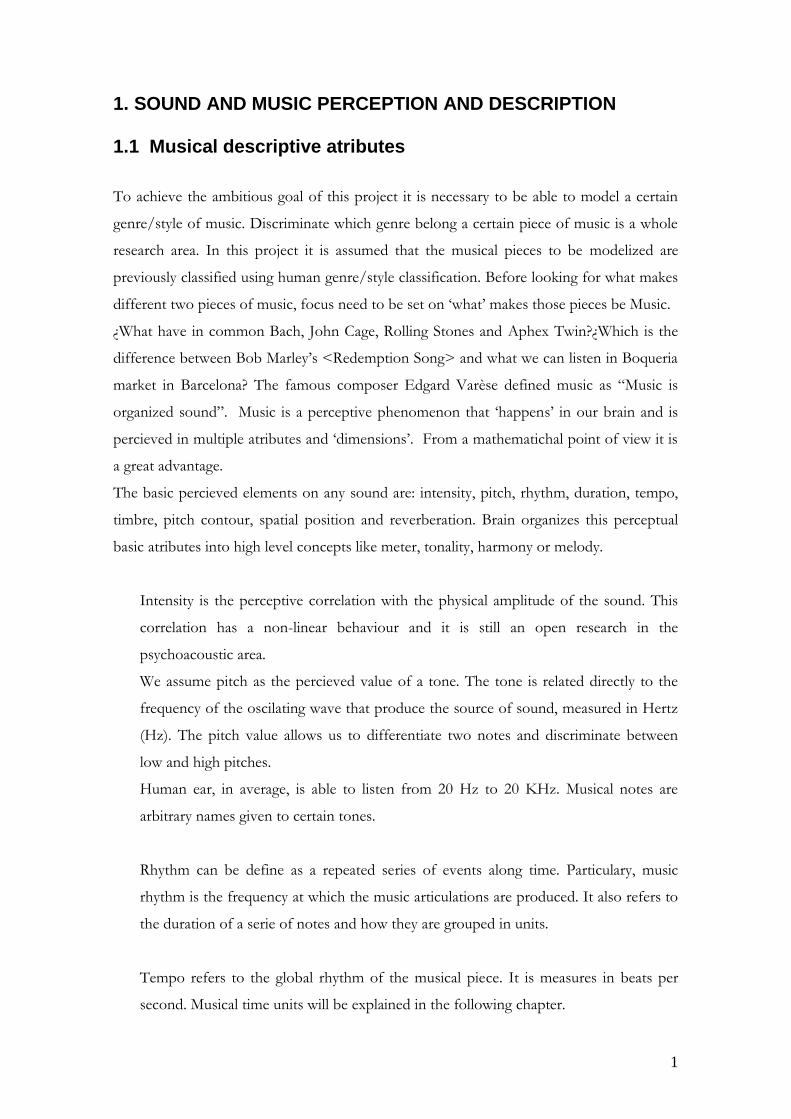
a) Rhythmic units
Figure 2. Rhythmic figures relative values to pulse duration(beat). Image from jesuscfk.blogspot.com
In order to write rhtyhm so it can be reproduced by a performer, an arbitrary measure
system has been formalized since Classical music era. The system is based on a relative time
relationship between the figure duration and the pulse duration(see Figure 2).
To control the ‘speed’ of the rhythm when it needs to be performed is measured in beats
per minute (bpm).

5
b) Metrical structures When listening to music, there’s a need in the listener to move their feet,hand or head
following some articulations. This first level of rhythm percieved is know as pulse or beat.
In a musical phrase some of the beats tend to be strong or accented while another are
weak. Meter perception depends on how a sequence of strong and weak pulses is
organized. All music based on a hierarchy of pulses has a meter. The time interval between
two strong pulses is called in musical lenguage bar. Depending on how rhythmic events are
distributed in a bar measure it can induce two different pulse subdivision perception. The
subdivisions can be binary (simple) or ternary (compound). For instance, if there’s a
perception that pulse is subdivided in two or four divisions it will be binary, if three
divisions are percieved it will be ternary.
In musical lenguage meter also called time signature is represented by a fraction. The
fraction numerator refers to the number of pulses, while the denominator set the units of
the pulse. In binary time signatures the denominator refers to the figure that measures the
pulse,while in ternary it refers to the figure that correspond to the subdivision of the pulse.
Without meter information, determine if an onset is syncopated or not becomes in an
ambiguous result[3]. The use of meter hierarchies allows musicians to use syncopations to
vary the predictability of a rhythm that otherwise is not possible[2].
c) Time signatures and genres
Figure 3 . Different time signature examples in musical notation. Image from ww.cnx.org
Along history many time signatures had been used (i.e. see Figure 3), and some of them are
shared in most musical pieces that share the same genre. For instance, most of the western-
music use a 4/4. In especific EDM genres like House or Techno this time signature i used
to generate a fondation rhythmic pattern known as ‘four-on-the-floor’. While 4/4 is the

6
default metric for electronic dance music, there are some artist that experimented with
other time signatures (i.e. see [10]).
1.4 The bass in electronic dance music The algorithm proposed in this project is focused on the study of electronic dance music
genres from a computational point of view, and more specifically the bass instrument.
EDM is the US terminology to refer to music genres such as House, Techno, Trance, and
other[13], so it’s not a genre itself [8]. Musical pieces that belong EDM are composed
thinking of a continuous context, where a DJ creates a continous mix using different music
pieces. In the ‘EDM terminology’ music pieces are called ‘tracks’ and not ‘songs’. This
multiple genres grouped under EDM are very popular in nightclubs, festivals and parties in
general.
Nowadays, there are limited references about generative music composition [1], and even
less about Electronic Dance Music computational study []. In order to make
interpretations of the proposed algorithm results is necessary to have a knowledge about
electronic dance music and it’s main subgenres. It’s also interesting to know how is the
enviroment of an electronic music musician/producer.
Figure 4. Acoustic bass. Image extracted from www.premierguitar.com
Figure 5. Roland Bass synthesizer TB-303. Image extracted from www.digitalstudent.co.uk

7
Like in the classical era, ‘traditional’ western-music and electronic music use some kind of
bass instrument. From acoustic basses (see Figure 4) to bass synthesizers (see Figure 5), the
bass represents the lowermost notes of a musical piece. Bass act like a harmony support,
and in dance music bass plays a very important role as rhythmic instrument. Bass phrases
are also known as basslines .
Genres like House and Techno sets their foundation on a 4/4 drum pattern and a clear and
heavy bassline as main elements of the track. Bassline together with the drums (i.e. Kick,
snare, clap, hi-hats, and others) set the rhythmic foundation of a track.
a) House Music
House Music [11] is a electronic dance music genre originated in the early 80’s in Chicago .
In the mid-80’s it became popular in other scenes like Europe or South America.
Nowadays, House music has been infused in mainstream pop and dance music worldwide.
From it’s popularity worldwide, House has been fusioned with other genres to create
subgenres i.e. Deep-House, Tech-house, Bass House and many others. Defining the genre
then becomes very difficult due to it’s multiple influences and fusions.
b) Techno
Techno music [12] is originated in Detroit in the middle 80’s. Now, exists many differents
kinds or subgenres of Techno which foundation is considered to be Detroit Techno. It’s
mainly an instrimuntal and composed in a context of continuous performance (i.e. DJ
performance). A main overall aspects of the Techno style and aesthetic are: emphatization
of rhythm over other parameters (i.e. harmony), design of synthetic sounds and a creative
use of technology. Techno use syncopated rhythms and polyrhythms to create a
charachteristic ‘groove’ feeling.

8
9
2. MUSIC RHYTHMS FAMILIES THEORY
The analysis algorithm is based on a recent article [5] that proposes grouping rhythm
patterns in families combined with the use of syncopation level [3].
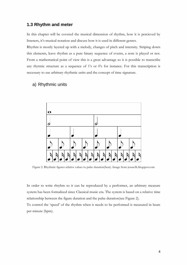
2.1 Syncopation level Longuet-Higgins and Lee in 1984 proposed the syncopation level, based on assigning
weights to the notes on a musical phrase according to their rhythmic relations with their
preceding notes. Syncopation level is the weight difference between a note and the silence
after it using a weight salience function profile. Longuett-Higgins and Lee proposed the L
weight profile (see Figure 6) to compute the syncopation level. Ladinig in 2009 proposes a
variation of the weight profile, using different profiles based on subject studies [6].
Figure 6. L weight weight profile proposed by Longuett-Higgins and Lee
Syncopation level has been used as a rhythmic similitude measure [3][6][7]. According to
perceptive experiments [4][6], syncopation level is related conceptually with rhythmic
complexity. Those experiments report a correlation between the syncopation level of a
rhythmic phrase and the difficulty of the subject to reproduce it. Syncopation level is used

10
as similarity measure in Tutzer’s [7] experiments with an accuracy of 76.6% of human
percieved similarity.
2.2 Rhythmic families In 2014 Cao et al. (2014)[2] proposes a perceptual measure of rhithmic similarity. Authors
propose to group rhythms in families based on their level of syncopation. The analisys is
only based on the ‘pattern of onsets’ of the rhythm, wich only have information about
inter-onset-intervals. The family theory makes five principal predictions[2]:
- If two rhythms share the same pattern of onsets, then they should tend to be
judged similar
- If two rhythms are from the same family, with other parameters being equal, they
should be judge as more similar than two rhythms from different families.
- If individuals try to reproduce a rhythm, their errors should tend to yield rhythms
in the same family as the original target as opposed to rhythms in a diferent family.
- Errors in reproduction should be more likely to occur in the case of syncopation.
- The fewer notes in a rhythm, easier it should be to be reproduced.
In the article, it is proposed to use a symbol to determine if a note/silence reinforces the
beat (N), is a syncope (S) or neither (O). Rhythmic families are those that share a same kind
of syncope within a given time resolution. An example of rhythmic family can be: ONON,
NNNN, and so on. Similarity between rhythms depends on both their temporal patterns of
onsets and their families [2]. Cao and Lotsein article shows that slicing a pattern into beats
and assigning family values to each beat according to their syncopation level, can be much
more accurate, in terms of rhythmic similarity, than using other measures like the edit
distance. That’s because family analysis takes into account especially meaningful musical
attributes such as syncopation. Analisys can be performed at different resolutions to have a
fine precision syncopation level. For instance, assume a bar length rhythm (in a 4/4 meter)
that at a quarter-note resolution it’s familiy is: NNNN. If the rhythm is analyzed at a
resolution of eigth-notes, syncopation between beats can be detected (i.e. NSNSNSNO).

11
3. METHOD The goal of the presented algorithm is to model a certain genre based on rhythmic
properties. The rhythm family theory in combination with the syncopation level will be
applied to make an analisys based on music perceptual features such as syncopation.
First step will be the creation of different data-sets containing MIDI bassline files. Each
data-set will belong to a specific genre or subgenre, and will be treated as a collection.
A weight profile to compute syncopation level will be proposed and used to compute
syncopation level in every beat measure for each loop. Once the syncopation level is
computed for every beat, of every loop in the data-set, is possible to group patterns that
share the same syncopation level in families. A probabilistic model will be proposed based
on the histograms of resulting families for every beat. For instance, it will be possible to
know the family rhythms distribution in a certain beat. The resultant probabilistic model
will feed a generation algorithm. Two approaches are presented. The first uses the family
distribution of each beat, and it’s pattern density distribution to generate basslines of a
given lenght. Second aproach takes in account a binomial relationship between the beats
rhythmic families.
3.1 Data-set selection The data-set is based on a selected collection of bassline loops. The collection of loops
must share a style/genre similitude. We decided to use commercial MIDI loop packs from
most reputed companies as Delectable Records1 , 5Pin2 , among others. These packs can be
found in Beatport Sounds3 and Loopmasters4 websites. Those websites offer product
preview clips that were used to make our selection. Most clip previews are based on
basslines samples from the collection, mixed together with a musical context such as
drums, pads and other sounds. The offer of such MIDI packs is quite limited, and even
more the MIDI basslines packs. A selection of MIDI basslines from the mentioned sources
are used to create five different data-sets.
1 http://www.loopmasters.com/labels/33-Delectable-Records 2 http://www.5pinmedia.com/ 3 http://sounds.beatport.com/ 4 http://www.loopmasters.com/
12
a) Deep-House data-set
The data-set is composed of 412 bassline MIDI loops from various commercial
loop packs. All loops are supposed to belong to deep-house genre. The beat lenght
of the collection is variable from 2 bars to 8 bars. Some of those packs include
other MIDI and audio material like drum loops, percussions and chord
progressions that will be very useful to study the musical context of those loops in
future steps This colection was validated by famous EDM producer and
discography owner Julio Navas[]. The following packs compose the data-set:
● Riemann Kollection Analog House Basslines 15
● Delectable Records Deep House Midi Basslines6
● Delectable Records Deep House Mega MIDI Pack 1 7
● Technique Sounds Deep House Studio Inspirations8
● 5Pin Media Deep House Bass9
b) Techno data-set
This data-set is based on a single large library of MIDI basslines called “5Pin
Bassline the Sequel 10 “. Its a collection that its description says it’s focused on
genres such as House, Tech House, Techno, Minimal, Trance. As explained, the US
originated term EDM encapsulates this genres. There’s a total of 354 bassline
loops, grouped in 3 different styles: classic & techy, deep & funky and hypnotic &
minimal(see figure 7).
5 http://sounds.beatport.com/pack/analog-house-basslines-1/8482 6 http://www.loopmasters.com/genres/50-Deep-House/products/3360-Deep-House-MIDI-Basslines 7 http://www.loopmasters.com/genres/50-Deep-House/products/3173-Deep-House-Mega-MIDI-Pack-1 8 http://sounds.beatport.com/pack/deep-house-studio-inspirations/7149 9 http://www.loopmasters.com/products/2253-Deep-House-Bass 10 http://www.loopmasters.com/genres/79-Bass/products/3061-Bass-Line-The-Sequel

13
Number of
loops
Percentage from
total
Classic & Techy 91 25,71%
Deep & Funky 106 30%
Hypnotic & Minimal 157 35%
Figure 7. Distrubution of different styles in Techno data-set
c) Tech-house data-set
This data-set is based on the collection from Delectable Records “Tech House
Monster MIDI Pack 0111”. This collection only contains 36 basslines that belong to
tech-house genre.
For the scope of this project, MIDI files will be transcribed to binary rhythms using the
MIDI note onsets. Those binary rhythms can be quantized at different resolutions. With
those binary rhytmic representations of the basslines will be applied the rhythmic analysis
to create a probabilistic model of the data-set.
3.2 Customizing rhythmic families theory In order to design the bassline algorithm, is presented a novel method to compute families
of rhythms combining the theory of rhythmic familes (Cao, Lotstein ,2014) and the
weighted rhythmic interpretation, proposed by Longuet-Higgins and Lee, with a
probabilistic model.
Basslines in collection are assumed to follow a 4/4 metronome. This assumtion is based on
the fact that the data-sets belong to EDM genre (see previous chapter). Longuet-Higgins
and Lee, syncopation level to group rhythms in families, based on Cao et al. (2014), is a
good start to analyze all loops in the collection.
11 http://www.loopmasters.com/genres/66-Tech-House/products/3651-Tech-House-Monster-MIDI-Pack-01

14
As stated by Longuet-Higgins and Lee, a ‘metrical unit’ need to be designated. Analyze
rhythm structures slicing them in beat units makes possible a more precise rhythmic
features extraction than using whole bars. The chosen ‘metrical unit’ will be the root of a
metrical hierarchy, which branches will depend on the assumed time signature or meter. In
the concerning case of 4/4 time signature the metrical hierarchy will result on a finite
binary tree. Authors’ proposal is to analyze the rhythmic structure confined in a bar
measure using a weight salience function. The L weight profile proposed by Longuett-
Higgins and Lee [3](see figure 8) can be used to compute syncopation level for each onset
of a given beat measure rhythm.
Figure 8. L weight weight profile proposed by Longuett-Higgins and Lee
Syncopation level is the weight difference between a note and the silence after it. Notes
followed by silences on uneven positions have negative values and are not considered
syncopations. Notes followed by silences on even positions have positive values and are
considered syncopations. The main idea is to know ‘how much’ syncopation there is in a
rhythmic structure preserving the syncopated event position in the phrase given the weight
of the onset in the resulting syncopation level.
Recently proposed family theory of rhythms [2 propose that note/silences in a rhythmic
sequence must belong to only one of the following categories: S for syncopation, N notes
on the beat, O for other events. Those categories are used to group rhythms with the same

15
string of categories (i.e NNNO, NNNN, NSOO, and so on). This categorization can be
adapted as follows: the resulting values, given by the syncopation level computation, of a
given rhythm are the strings to generate the families. Instead of proposed families [2](i.e
NONO) it is proposed to use syncopation level to group rhtyhms (i.e. -2 0 -1 0).
Given that the negative values of the syncopation level represents notes that reinforce the
beat and positive values notes that represent syncopation, is possible to measure the
similitude of two rhythms. The similitud is computed comparing the sum of the resulting
syncopation levels of each rhythm.
The choice of analysis resolution can not be arbitrary. A new weight profile is proposed
after facing the problem of setting its size. The size of the used weight profile determines
the resolution at which the beat measure will be analyzed. For instance, with a 16 size
weight vector allow to analyze with a 1/16 beats resolution. To choose the right analysis
resolution the target collection (deep-house data-set) will be analyzed at different
resolutions.
Syncopation L weight level is a 16-weights array so the beat must be divided with such
resolution, ¼ beat or 1/64 bars to be analyzed. 1/64 bars resolution is accurate enough to
make an initial family computation. Once syncopation level is computed at 1/64 resolution
it possible to get the syncopation level at a double resolution, downsampling the resultant
syncopation level by factor 2. The obtained syncopation levels will be treated as strings
and grouped in families using a histogram. In our selected bassline loop collection, the
variance of family histograms from 1/64 to 1/16 bar resolution are the same, in upper
resolutions decrease. Highest variance in the family histogram means more variety of
families are found in that resolution. 1/16 bars resolution is the optimal analysis resolution
for the selected collection. In fact, rarely a bassline can be played using notes sequences
shorter than 1/16.
The algorithm is going to analyze the collection at 1/16 bars resolution, 4 divisions per
beat, beacause it’s a reasonable precise resolution to extract basslines information. L weight
profile must be applied to every beat sliced in sixteen divisions (1/64 bars resolution). That
means that it is not suitable to compute our model and therefore it is necessary to design a
new weight profile in order to analyze beats sliced in 4 divisions, at 1/16 bar reolution. The
new weight profile to compute syncopation level must keep the same theoretical
16
background as Longuet and Lee syncopation level, it will be called S weight profile. The S
weight profile must assign unique values to every slice depending how it contributes to
syncopation or beat reinforcement, depending on the onset position inside the beat [3].
Notes on first and third division of the beat reinforce the beat so the weight assigned to
them must be negative. Notes on second and fourth division are syncopations and then
weights will be positive. Notes on first division reinforce more the beat than the third, and
notes on the fourth syncopates more than in the second. Using a range between -2 and 2
for the weights we can build the new profile. Number 0 as a resultant weight mean the
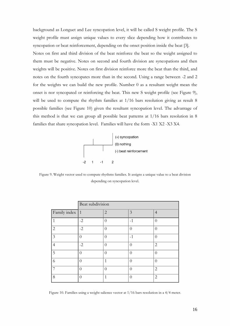
onset is nor syncopated or reinforcing the beat. This new S weight profile (see Figure 9),
will be used to compute the rhythm families at 1/16 bars resolution giving as result 8
possible families (see Figure 10) given the resultant syncopation level. The advantage of
this method is that we can group all possible beat patterns at 1/16 bars resolution in 8
families that share syncopation level. Families will have the form -X1 X2 -X3 X4.
Figure 9. Weight vector used to compute rhythms families. It assigns a unique value to a beat division
depending on syncopation level.
Beat subdivision
Family index 1 2 3 4
1 -2 0 -1 0
2 -2 0 0 0
3 0 0 -1 0
4 -2 0 0 2
5 0 0 0 0
6 0 1 0 0
7 0 0 0 2
8 0 1 0 2
Figure 10. Families using a weight salience vector at 1/16 bars resolution in a 4/4 meter.

17
Most families contain obviously more than one pattern (see Figure 11). Patterns grouped in
the same family are more similar in a perceptive way between them than to patterns from
other families. Multiple patterns from a family differ on their number of onsets. For
example: a beat measure associated to the family with syncopation values [2 0 0 -2] can
contain 2 possible patterns. Those patterns are X00X and X0XX and their respective
number of onsets are 2 and 3. Must be mentioned that same patterns can belong to
different families, depending on the onset values of the next beat.
The probilistic model will be based on the following statement: given a family and a
suitable density value, we can obtain an unique pattern. Using this last observation we can
design a simple model, based on family and density probability distribution functions for
every beat, in order to model every beat measure. The probability distribution is computed
using the historgram of the number of ocurrences of each family per every beat. The
histogram must be normalized to become a discrete probability function. Same
normalization method is applied to the density histogram for every beat.
Pattern density
Family
index 0 1 2 3 4
1 1010
2 1000 1001 1011
3 0010 0110 1110
4 1001 1011
5 0000 0001 0011 0111 1111
6 0100 1100,0101 1101
7 0001 0011 0111 1111
8 0101 1101
Figure 11. Corresponding patterns given Family index and pattern density values.

18
3.3 Method tools Analysis and generation code is implemented in MATLAB and is still in development. To
manage midi files a reputed third-party toolbox is used: Matlab MIDI Toolbox developed
by Jyvaskyla University allows to read, write and manipulate MIDI data [1]. This toolbox is
very useful to transcribe MIDI files into symbolic rhythmic sequences.
3.4 First approach: ‘blind’ analysis
Figure 12. Block diagram of the ‘blind’ analysis/generation method
First approach takes into account two statistical models:
- Family probability distribution across beats
- Density of onset of every family across beats
This analysis allows us to analyze the differences in families distributions across every beat
measure. Consequently, computed probabilities for every beat measure are independent
between them; computations are ‘blind’ to other beats. This model is able to generate
indivdual beats with a family distribution according to the desired beat, but don’t extract
any information on how beats are related (see Figure 12).
From the family distribution in every beat measure we can obtain very useful information.
A first hypothesis can be that family distribution is not the same in every beat measure.
Another hypothesis is that depending on the beat position, family distributions will tend to
focus in certain families. Detect if some beat positions share similar family distributions can
be very useful to model the genre and extract high-level features to model it.

19
The files are analyzed sequentially. The collection needs a pre-analysis before building the
model used to generate new MIDI files. This pre-analysis consists on the following steps:
First, MIDI file is quantized to 1/16 bars (analysis resolution). Quantizing the file, ‘groove’
timing information is lost, but for the moment this is not taken into account. The
quantized file is converted to a binary vector with 4 divisions per beat measure. Beat
divisions that contain an onset are set to 1, others to 0. All onsets are assumed to have
regular length, in this particular case 1/16 bar. Once all files are binarized, it’s necessary to
struct the files to analyze them properly. The family analysis is made for every beat, so it is
necessary to set a matrix per every analyzed beat(see Figure 13). These matrices will contain
all rhythmic patterns found in the associated beat. We will call this data structure ‘per-beat’
in the text below. That means that the analisys is realised for every independently, storing
the given results depending on their beat position (i.e. all first beat measures of all loops
will be stored in a single matrix).
N beats
1 2 3 4 … N
Bassline 1 [XXXX] [XXXX] [XXXX] [XXXX] [XXXX] [XXXX]
Bassline 2 [XXXX] [XXXX] [XXXX] [XXXX] [XXXX] [XXXX]
Bassline 3 [XXXX] [XXXX] [XXXX] [XXXX] [XXXX] [XXXX]
Bassline 4 [XXXX] [XXXX] [XXXX] [XXXX] [XXXX] [XXXX]
Bassline 5 [XXXX] [XXXX] [XXXX] [XXXX] [XXXX] [XXXX]
… [XXXX] [XXXX] [XXXX] [XXXX] [XXXX] [XXXX]
Bassline M [XXXX] [XXXX] [XXXX] [XXXX] [XXXX] [XXXX]
Figure 13. Data structure to analyze collection.
Data is ready now to compute rhythm families. They are computed for every beat of every
loop (every column in matrix in Figure 13) and the results are stored as a Syncopation
Matrix. This matrix has a per-beat structure (see Figure 13).
Now it’s possible to know the overall family histogram. From this histogram we will obtain
the rhythmic families contained in the collection and its probability distribution. Indexing
the found families in the collection allows making a more structured family analysis for
each beat measure. Refer to familys using an unique index to family correspondances allow

20
to compare the results. Moreover, information like the bar lenght of the loops in data-set
can be easily obtained.
Once this simple model is computed we are able to design a generator based on it (see
Figure 12). The explained analysis is computed offline and the users only need to set the
input data-set collection.
The generation is based on family and density statistical knowledge extracted from the
selected collection of basslines. A big shortcoming of this method is that we are analyzing
beat measures independently, so any possible beat relationship knowledge is lost.
It’s important to point that, for a correct family computation of a certain beat, the first ¼
beat measure of the next beat is required when; in case the last beat is being computed,
loop phrase is assumed and the first ¼ beat measure in the loop is used. So, there is no
relationship between beat families considered. To improve this simple ‘blind’ model
relationship between consecutive families must be considered.
a) Pseudocode
The analysis pseudocode is the following:
for each MIDI file in data-set
x = Quantize (MIDI file)
binary rhythm = ‘Binarize’(x)
for each beat in the binary rhythm
y = Compute rhythmic family (syncopation level) with S weight profile
Store (y) in SyncopationMatrix(beat)
Store density depending on rhythmic family
end
end
for each beat
Compute family pdf from SyncopationMatrix(beat)
Compute density pdf from stored values for each beat and family
end
The generation algorithm pseudocode is the following:
21
for each beat
f = random sample family pdf
d = random sample density pdf ( f )
GeneratePattern (f,d)
end
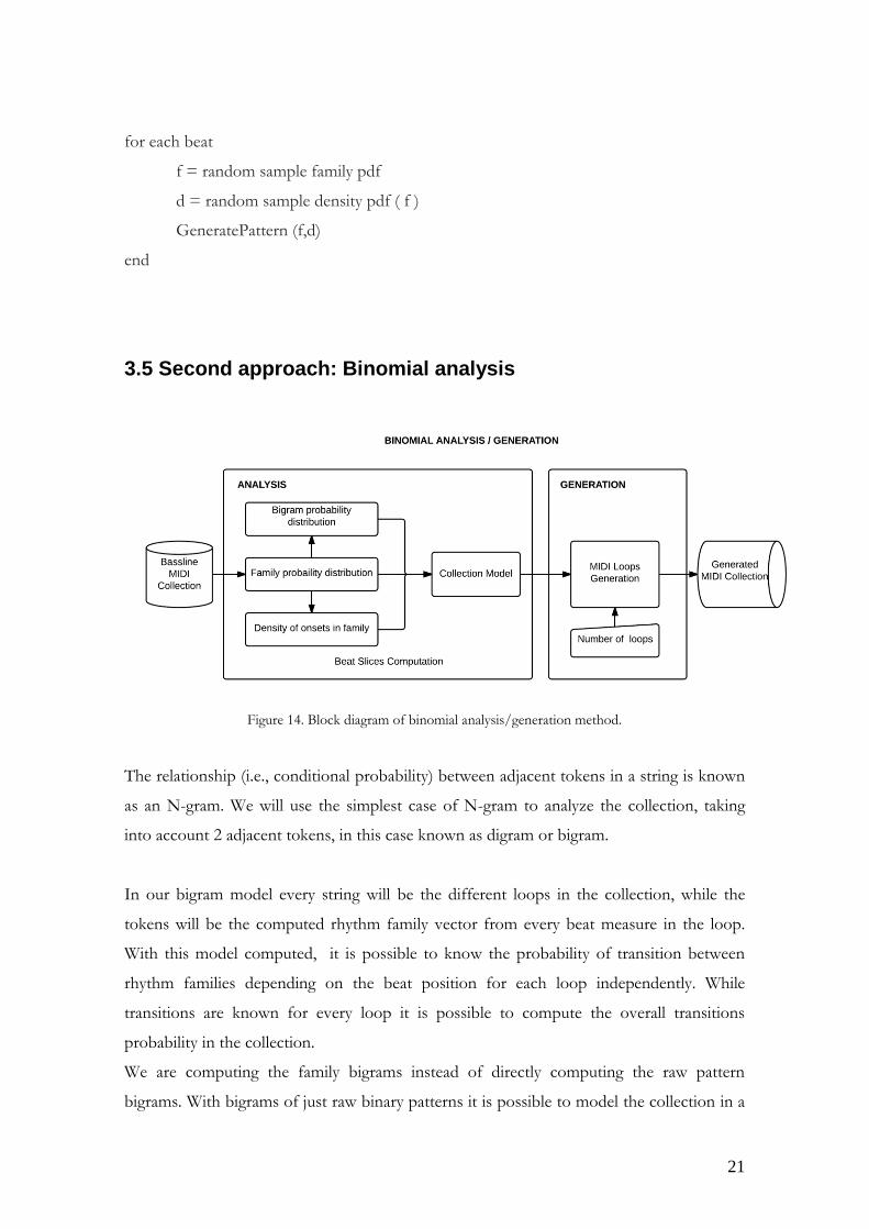
3.5 Second approach: Binomial analysis
Figure 14. Block diagram of binomial analysis/generation method.
The relationship (i.e., conditional probability) between adjacent tokens in a string is known
as an N-gram. We will use the simplest case of N-gram to analyze the collection, taking
into account 2 adjacent tokens, in this case known as digram or bigram.
In our bigram model every string will be the different loops in the collection, while the
tokens will be the computed rhythm family vector from every beat measure in the loop.
With this model computed, it is possible to know the probability of transition between
rhythm families depending on the beat position for each loop independently. While
transitions are known for every loop it is possible to compute the overall transitions
probability in the collection.
We are computing the family bigrams instead of directly computing the raw pattern
bigrams. With bigrams of just raw binary patterns it is possible to model the collection in a

22
‘deaf’ way without any perceptual or musical meaning. On the other hand, work with
rhythm families will allow us to analyze those transitions in a musically meaningful way. As
we said, a family mostly group more than one pattern so computing families transitions
gives a bigger range of ‘possible’ generated paterns than only computing transitions with
the raw patterns
Now, the ‘next-family’ choice made by the generator algorithm will be influenced by: the
current family and the bigram model. The simple version of the generator (see previous
section), explained previously, is used to choose the ‘seed’ family for the first beat. Once
the first beat pattern is generated using correspondent family and density probability
distribution functions, the rest of beats will be based on bigrams found in collection.
Following patterns will be generated using correspondent bigram model and density
distribution function as seen in Figure 14.
a) Pseudocode
The generation pseudocode for the binomial approach is the following :
for each beat
if 1st beat
f(n) = random sample family pdf
d(n) = random sample density pdf ( f(n) )
else
f(n) = random sample bigram pdf ( f(n-1) )
d(n) = random sample density pdf ( f(n) )
end
GeneratePattern (f(n),d(n))
end

23
3.6 Generation control parameters
In order to generate basslines using the exposed algortihm are necessary the following data:
As result of the analysis:
Family probability distribution function (for every beat)
Density probability distribution function (for every beat and family)
Binomial model (for each beat)
User controls:
Beat lenght of the generated bassline
Probability threshold
Above parameters are already covered, in exception of the probability threshold. The idea
is to set a relative threshold to filter the probability distributions as a low-pass, high-pass,
or using two thresholds as a band-pass. Filter the probability distributions will allow to
‘select’ ranges of the distribution, and for instance, avoid less common families or only use
the most ‘rare’ ones. This parameter can be a very useful parameter to allow the user
interacts in the generation proces.
3.7 Results
First and second approaches of analysis/generation share most of the processes with the
exception of the bigram model, which is exclusive of the second approach. In this section
the results given by implementing both aproaches of the algorithm will be discussed.

24
a) Family distribution
Once a data-set is analyzed it is possible to compute the overall hisogram of the different
families ocurrences found in the collection. From this histogram the probability density
function of families in the whole collection can be calculated. This overall family
distribution can be a good descriptor to discriminate between genres and needs a deeper
study.
Figure 15. Probability distribution of families found in the deep-house collection from the 8 possible families
(see Figure 11).
Loops in collections have different beat lengths. In deep-house collection only 2% of the
loops were longer than 4 bars. In order to avoid a model extracted from a small amount of
data, only 4 first bars of every loop results will be studied in this case. As shown in Figures
15-,19 all possible families (8) are found in the deep-house collection and it’s associated
probability. In Figure 15 the distribution shows that the more syncopated families (index >
5) are less prominent than families that reinforce the beat. Due to the quality and amount
of data we will consider this data-set as a reference to test with users (see chapter
evaluation).

25
The classic&techy data-set distribution (see Figure 16) shows a predominance of the
syncopated families. The predominance of the syncopated families correspond to the
classic foundations of Techno music. Another observation is that the family with higher
beat reinforcement patterns and the most syncopated family have a very low probaility
compared to the other families.
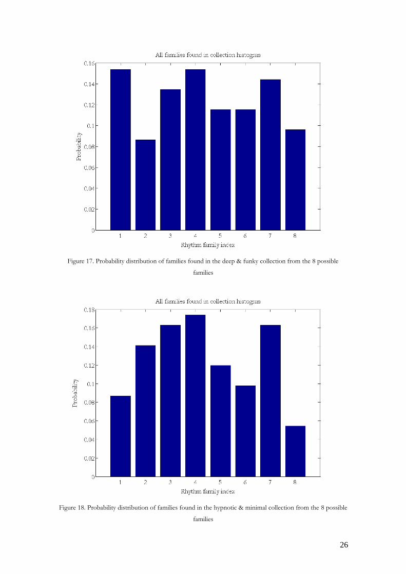
The deep&funky data-set distribution (see Figure 17) has a noticiable similitude with the
deep-house set distribution(see Figure 15). A more exhaustive comparison between this
two data-sets can be relevant to model “deep” music descriptor. Same qualitative
description can be applied to the other data-sets. For the moment, data-sets (except deep-
house data-set) are not big enough to extract reliable conclusions.
We can forward the hypothesis that different styles/genres will have different overall
family distribution as seen en Figures 15-19 (but testing that is still a matter of future work,
involving the analysis of other collections).
Figure 16. Probability distribution of families found in the classic & techy collection from the 8 possible
families.
26
Figure 17. Probability distribution of families found in the deep & funky collection from the 8 possible
families
Figure 18. Probability distribution of families found in the hypnotic & minimal collection from the 8 possible
families

27
Figure 19. Probability distribution of families found in the tech-house collection from the 8 possible families
b) First approach results: ‘blind analisys/generation’
Computing the family histogram for every beat independently, using the Syncopation
Matrix, makes possible to analyze the family probability distribution across beats. And,
more importantly, indexed families allow comparing the histograms of every beat. Blind
analisys is computed for the five data-sets. Following histograms (see Figure 6,7,8,9,10),
show the discrete family probability distribution function for each beat.

28
Figure 20. Each histogram shows the histogram of rhythmic families distribution for it’s associated beat in
deep-house data-set. Y-axis represents probability and X-axis represent the 8 rhythmic families.
This per-beat analysis allows studying the syncopation behaviour of the different beat
measures in this particular style/ genre, (see Figure 20, where the selected collection shows
similar distributions for some beats that share position inside the bar). For example, we can
see in Figure 6 that beats in the first position of the bar tend to contain patterns from
families that reinforce the beat. Other beats like 2 and 6 have a ‘most common’ family
compared to others like 15 that probability is very distributed around families. Using the
other data-sets, it is possible to compare their distributions per beat. As said before,

29
Figure 21. Each histogram shows the histogram of rhythmic families distribution for it’s associated beat in
tech-house data-set.
Figure 22. Each histogram shows the histogram of rhythmic families distribution for it’s associated beat in
classic & techy data-set.
Figure 23. Each histogram shows the histogram of rhythmic families distribution for it’s associated beat in
deep & funky data-set.

30
Figure 24. Each histogram shows the histogram of rhythmic families distribution for it’s associated beat in
hypnotic & minimal data-set.
These probabilities (see Figures 20-24) are used to generate patterns for every beat using a
statistical model based on musical meaningful attributes such as syncopation. To know the
family distribution for every beat give us information abouts it’s syncopation level, but
there’s a very important information missing using this model. Density of onsets in the
pattern, as said, is the parameter that allows differentiating patterns that share syncopation
level. A probability distribution function for density is computed depending on the beat
position and family. That means for every beat and every family, an onset density
probability distribution is computed. From this computed density probability distribution
we can compute the probability distribution of density in every beat without caring about
families, but it gives relevant information about how density is ditributed depending on
beat positions (see Figures 25-29).

31
Figure 25. Density distribution for patterns in every beat without family discrimination for the Deep-house
data-set(First 2 bars).
Figure 26. Density distribution for patterns in every beat without family discrimination for the classic & techy
subdata-set(First 2 bars).

32
Figure 27. Density distribution for patterns in every beat without family discrimination for the deep & funky
subdata-set(First 2 bars).
Figure 28. Density distribution for patterns in every beat without family discrimination for the hypnotic &
minimal subdata-set(First 2 bars).

33
Figure 29. Density distribution for patterns in every beat without family discrimination for the Tech-house
data-set (First 2 bars).
Both computed statistical models, family and onset density, are used to feed the first ‘blind
generator’. This first approach program analyzes the collection to build the model. Using
the model we can generate loops of various lengths. The length of those will be restricted
by the size of the extracted model. The MIDI generated files only contain valuable
rhythmic information, nor pitch or velocity.
The current evaluation is based on subjective listening only, where the members of the GS-
MTG have been judging the generated patterns. The patterns were played by a bass
synthesizer patch, mixed with a drum loop to give a context, with the possibility to monitor
the tracks separately. The results sounded quite random.
For a proper evaluation of the generated results a group of expert users will be used in
future steps of the project. This group of users needs to be expert in the style/genre we are
working. Expertise is needed to be able to recognize style characteristics. Evaluation
techniques need to be improved in order to provide a solid subjective demonstration of the
achievements.
34
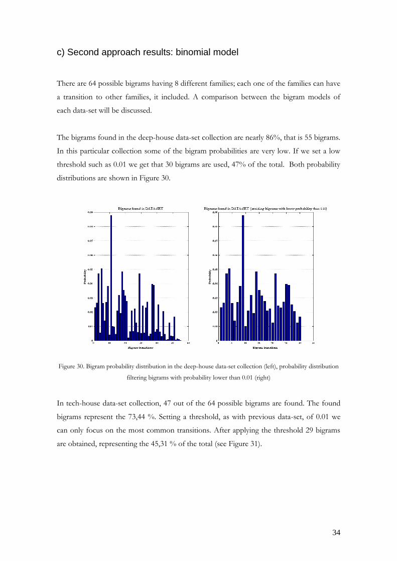
c) Second approach results: binomial model
There are 64 possible bigrams having 8 different families; each one of the families can have
a transition to other families, it included. A comparison between the bigram models of
each data-set will be discussed.
The bigrams found in the deep-house data-set collection are nearly 86%, that is 55 bigrams.
In this particular collection some of the bigram probabilities are very low. If we set a low
threshold such as 0.01 we get that 30 bigrams are used, 47% of the total. Both probability
distributions are shown in Figure 30.
Figure 30. Bigram probability distribution in the deep-house data-set collection (left), probability distribution
filtering bigrams with probability lower than 0.01 (right)
In tech-house data-set collection, 47 out of the 64 possible bigrams are found. The found
bigrams represent the 73,44 %. Setting a threshold, as with previous data-set, of 0.01 we
can only focus on the most common transitions. After applying the threshold 29 bigrams
are obtained, representing the 45,31 % of the total (see Figure 31).

35
Figure 31. Bigram probability distribution in the tech-house data-set collection (left), probability distribution
filtering bigrams with probability lower than 0.01 (right)
In classic&techy data-set collection, 22 out of the 64 possible bigrams are found. The
found bigrams represent the 34,38 %. Setting a threshold of 0.01 we can only focus on the
most common transitions. After applying the threshold 9 bigrams are obtained,
representing the 14,06 % of the total (see Figure 32). In this collection the bigram analysis
shows that there’s not as much variation as in the other data-sets.

36
Figure 32. Bigram probability distribution in the classic&techy data-set collection (left), probability
distribution filtering bigrams with probability lower than 0.01 (right)
In deep&funky data-set collection, 50 out of the 64 possible bigrams are found. The found
bigrams represent the 78,13 %. Setting a threshold, as with previous data-set, of 0.01 we
can only focus on the most common transitions. After applying the threshold 30 bigrams
are obtained, representing the 46,88 % of the total (see Figure 33).
Figure 33. Bigram probability distribution in the deep&funky data-set collection (left), probability distribution
filtering bigrams with probability lower than 0.01 (right)
In hypnotic&minimal data-set collection, 44 out of the 64 possible bigrams are found. The
found bigrams represent the 68,75 %. Setting a threshold of 0.01 we can only focus on the
most common transitions. After applying the threshold 26 bigrams are obtained,
representing the 40,63 % of the total (see Figure 34).

37
Figure 34. Bigram probability distribution in the hypnotic&minimal data-set collection (left), probability
distribution filtering bigrams with probability lower than 0.01 (right)
All the sub-data-sets of the techno (see Figures 32-34) data-set show a common property.
If we look at Figures 32-34 it’s noticable that there is a predominant transition in the
collection. In the three data-set the predominant transition is the same, from family index 4
to family index 4. Family index 4 correspondant possible patterns are 1001 and 1011 (see
Figure 11), and it’s syncopation level is [-2 00 2]. For this particular family, if we sum the
syncopation level is obtained 0. This result can drive to the wrong interpretation that nor
beat reinforcement or syncopation is happening [3], but it’s not. This family contain an
onset with maximum beat reinforcement and maximum syncopation. This particular family
and it’s significance will be a thread of research in future steps. Working with this three sub
data-sets (classic&techy, deep&funky and hypnotic&minimal) could be a good start point,
due to the predominance of the concrete family of interest.
The family distribution across beats is implicit in the bigram model for every beat, so it is
only used to select the first family. Once a seed family is selected, the family selection in the
next beat will be restricted by bigram probability distribution in given beat. Algorithm then,
will work as a state-machine. A kind of visual plot like Figure 35 can be very useful to
represent bigram probabilities and for example be able to detect very easily peaks on
certain bigrams.

38
Figure 35. This coloured mesh represents the bigram probabilities between families in a certain beat. Y-axis
represents the predecessor family indices, so each row of the matrix is the family probability distribution for
next beat families. X-axis represents the indices of families. The legend shows the different probabilities.
Results using the bigram model are much perceptually better than with previous ‘blind’
method. Most of the generated loops ‘follow’ the style of the collection. In this case,
playing the midi generated loops, in a NI Massive patch in C2,and with a nice ‘agnostic’
drum loop to provide more musical context the feeling was really good. It’s conceptually
reasonable that the binomial model will ‘reach’ better result than the blind model. To prove
that, will be necessary to plan experiments using human subjects to evaluate ‘some-how’
the perceptual similitude between the original data-set basslines and the generated basslines
using the algorithm.

39
4. EVALUATION
4.1 Deep-House scoring experiment
a) Participants
Nine professionals EDM producers and performers, all of them men, volunteered to
participate in the experiment. They were recruited with the help of Julio Navas12, a valued
producer and DJ with over 20 years experience in the EDM scene. Including Julio Navas,
participated: Maris, Ivan Pica, Jaen Paniagua, One D, Aitor Contreras, Angel Gama,
Andrea Roma, Elio Riso. They perform and produce various genres, but manly those
derived from House and Techno. Moreover, they are supposed to have a musical
background. It is considered they are experts in EDM, which makes reasonable to work
with only nine participants.
b) Design
The main goal of the experiment is to evaluate if the algorithm is able to model a certain
genre based on rhythmic anlisys, for the moment only based on inter-onset intervals. The
selected genre to test the algorithm is Deep-House. The choice of this collection has two
reasons; First, it is the biggest data-set, so the model must be more ‘generic’ than with
smaller collections. Second, the data-set is aproved, by the experienced producer Julio
Navas, as a representative Deep-House collection.
User are asked about their musical knowledge expertise using a 5 degree scales, from
completely diagree to completely agree. They are asked about:
- Electronic music expert
- Deep-house genre expert
- Electronic music profesional
12 http://es.wikipedia.org/wiki/Julio_Nava_(m%C3%BAsico)

40
Thirty loops will be presented to the user sequantially, with a brief margin of time between
each loop. After listening each loop, the user is required to evaluate it in a 5 degree scale.
The user must score the loop depending on how much/less he thinks the rhythm phrase
belongs to Deep-House genre.
The different scores will be analyzed to determine the mode,media and average for each of
the three groups.
These are the instructions given to the users:
We are interested in what is it that makes "good" a loop of specific electronic music sub-
genres. Here we are dealing with deep-house. We would greatly acknowledge your
collaboration in this deep-house rating experiment that will not take more than 10 minutes
of your time.
Using headphones if available, listen to the examples below and rate each one
according to the goodness of fit to your idea of a good deep house bass loop.
Focus attention to the bass rhythm loop only and rate each one using the given
scale:
1: not at all deep house
2: unlikely deep house
3: unclear
4: deep house loop, probably
5: no doubt it is a deep house loop
You may find that some of the examples are probably good examples of deep-
house, whereas some other are no so good or unclear, and that there are even very
bad ones. Please, try to use the full range of rankings we give you. Have in mind
that here are no right or wrong answers, and that not all the examples might belong
to just one category.
Thanks for your collaboration.

41
c) Materials
Three groups of 10 loops are used in this experiment. So, there’s a total of 30 loops to
evaluate. All loops are 2 bars long.
- First group: contains random selected original loops extracted from the
collection. In order to be tested they are pitch flatened and the duration of the
notes is set to a semi-quaver.
- Second group: contains loops generated by the algorithm. As generation
parameters it was restricted only to use the most common values in the probability
distributions. A threshold is set such as, all probability values smaller than the half
of the maximum probabilty value are avoided. This filtering allow us to focus the
generation algorithm only on the most generic transitions. The avoided values are
supposed to be ‘rare’ transitions that are not useful to recreate the ‘generic’ rhythms
that characterize the genre.
- Third group: contain loops generated by the algorithm, but using a
equiprobable model for the transition probabilities and family distribution. This
group objective is to be the control group. It will be relevant when analyzing the
results, compared to the other two groups.
The experiment data-set is now composed by 30 MIDI files containing rhythmic
information about the Deep-House basslines data-set. All notes, in every file, are one semi-
quaver long , C2 note pich, with equal velocity.
In order to make the experiment in a musical context, the files need to be rendered and
layered with an ‘agnostic’ drum-track. Native Instruments Massive13 was used inside
Ableton Live14 to render the MIDI files. The patch selected, is called Hollow Bass and it’s
included in the Massive library, has ‘deep-house’ timbric features. On the other hand, a
simple combination of a tuned kick, clap, snare and hi-hats was used for the drum-track. At
the end, each bassline rendered is mixed with the same drum track. The resulting files order
is always the same for every user and it’s obtained sorting randomly the loops contained in
the three groups.
13 www.native-instruments.com/es/products/komplete/synths/massive/ 14 https://www.ableton.com/

42
The evaluation is thought to be online and self-tested, so it uses a webpage platform. The
webpage is allocated in Google Sites. The audio data-set is uploaded in Soundcloud15
service. Soundcloud allows creating reproduction playlists and embedding them as a widget
in a site. The users need to answer in a form, based on Google Forms service. This
experiment online environment allows broadcasting it and be shared easily.
d) Procedure
Evaluator user need to acces the experiment website. First thing user see are the
experiment intructions. Once the user is familiar with the instructions can proceed to the
experiment realisation. The playlist is presented in the left side of the screen, while in the
right side there is the evaluation form. Before starting the evaluation, the user needs to
answer the ‘previuous questions’. This ‘previous questions’ are to introduce a user name, an
optional e-mail, and answer the musical knowledg expertise questions.
Playlist reproduces the loops sequentially with a brief silence time enough to evaluate it. If
the user wants to listen again a specific loop it is possible without any restriction.
Figure 36. Website where is allocated the experiment. It’s URL is
https://www.sites.google.com/site/deephousinesstest/
15 https://soundcloud.com/user806478547

43
e) Results
To make a first evaluation of the results it will be computed some statistic measure using
the scores . The interest is to compare the ‘global score’ for each of the evaluated groups.
To compute ‘global score’ three basic statistic measures will be used: median, mode and
average (see Figure 36-37).
SUBJECTS SCORES STATISTICS
TEST FILES 1 2 3 4 5 6 7 8 9 MODE MEDIAN AVERAGE
generated1.mid' 3 4 4 3 2 1 2 4 4 4 3 3,00
generated10.mid' 4 1 2 2 4 3 4 4 4 4 4 3,11
generated2.mid' 3 3 2 3 4 2 4 4 4 4 3 3,22
generated3.mid' 3 2 1 2 4 1 1 4 3 1 2 2,33
generated4.mid' 4 1 3 3 5 2 3 4 4 4 3 3,22
generated5.mid' 4 3 3 4 4 5 4 4 2 4 4 3,67
generated6.mid' 5 4 3 4 4 1 2 4 2 4 4 3,22
generated7.mid' 2 4 4 4 2 3 3 4 5 4 4 3,44
generated8.mid' 3 2 1 2 2 2 1 4 2 2 2 2,11
generated9.mid' 2 5 3 3 2 4 1 4 4 4 3 3,11
original1.mid' 3 4 4 5 5 3 2 4 4 4 4 3,78
original10.mid' 2 4 4 4 4 1 3 4 4 4 4 3,33
original2.mid' 4 3 3 4 4 1 4 4 5 4 4 3,56
original3.mid' 4 4 2 4 2 3 1 4 4 4 4 3,11
original4.mid' 3 5 4 4 2 5 2 4 5 5 4 3,78
original5.mid' 4 4 3 4 3 3 1 4 4 4 4 3,33
original6.mid' 4 3 1 2 4 1 1 4 1 1 2 2,33
original7.mid' 3 3 4 3 4 2 5 4 4 4 4 3,56
original8.mid' 4 5 5 4 2 1 2 4 4 4 4 3,44
original9.mid' 3 4 4 4 3 5 2 4 4 4 4 3,67
random1.mid' 3 4 3 3 3 3 2 4 4 3 3 3,22
random10.mid' 4 3 2 4 1 2 2 4 4 4 3 2,89
random2.mid' 3 3 2 3 2 4 1 4 3 3 3 2,78
random3.mid' 4 3 3 4 5 4 3 4 4 4 4 3,78
random4.mid' 3 4 2 4 4 2 1 4 4 4 4 3,11
random5.mid' 2 4 1 4 3 2 1 4 4 4 3 2,78
random6.mid' 4 4 4 3 3 1 2 4 4 4 4 3,22
random7.mid' 4 2 1 3 3 3 1 4 5 3 3 2,89
random8.mid' 4 3 4 4 4 2 2 4 3 4 4 3,33
random9.mid' 4 3 2 4 3 2 3 4 3 3 3 3,11
Figure 36. Evaluation score results for every subject and evaluated file. Basic statistical measures are
computed for each evaluated file.

44
GROUP MODE MEDIAN AVERAGE
GENERATED 4 3 3,04
ORIGINAL 4 4 3,39
RANDOM 4 3 3,11
Figure 37. Evaluation score results statistics using all scores from the group.
Results for every group (see Figure 37) show very similar overall scores for each of the
groups. With a very small difference, the average and median of the ‘original’ group is
higher, but not as it was expected. ‘Generated’, ‘random’ and ‘original’ group have very
similar statististics. This results shows that the test is not reliable so it need to be replanned.
A second aproach is to extract the same information but only with the super-experts.
Super-experts were designated under Julio Navas criteria. Figure 38 shows the histograms
of the scores for each group, the above part include all subjects, the down part only the
super-expert. Results are still ambigous so the plan of another test will be required in order
to experiment further with the achieved results in this project.

45
Figure 38. Score results of the subject evaluation. Up are shown the histograms of the score results taking in
account all subjects. Down are shown the same results only for super-expert users.

46
5. NEXT STEPS
Short term steps are the deeper study of the analyzed data-sets and evaluate them with
expert users. For limitations of time it hasn’t been possible an exhaustive study of the
already done evaluation so will be continues.
Mid term steps will still be focused on rhythmic knowledge extraction. Perceptive relevant
features such as note duration and note velocity will be studied. The method to obtain a
statistical model of those features still needs to be discussed.
A first real-time prototype will be designed taking in account user interaction. Onset
density will be the first parameter to study in order to implement a ‘first’ user interaction.
Moreover to user interaction, an important goal of the project is that the algorithm is able
to ‘listen’ to some musical context. Generate rhythmic patterns that fit in a certain music
context will need a deep study in topics such as rhythmic similarity measures.
Next year I’ll continue with this project during the Master in Sound and Music Computing
in Universitat Pompeu Fabra.
User case example:
An electronic music producer, called James, is quite uninspired and is wasting the whole
morning to produce a proper bassline for a deep-house track. At least, he has an idea of the
overall style he wants to produce. So he goes to find a loop collection for some inspiration
on loop packs webstore. After looking for several collections he finds out one that fits with
his overall idea. With the collection in his hands he can look into many different loops,
choose one and drag it on his DAW. However, James wants to create a genuine track, and
using a loop from a commercial collection straightforward is not very genuine.
So it would be very useful to have an agent (see Figure 39) that can generate as many
basslines as you want based on a reference bassline collection, compared to spending time
on a trial and error process of note-after-note generation. In that same case, James could
also use his own genuine bassline collection from his old released tracks to generate new
basslines in James’ style. Independently from the collection chosen, James will save a lot of
time to invest on his projects and will obtain similar or even better results than following
more traditional techniques.

47
Figure 39. Outline of bassline agent

48

49
References
[1] Eerola, T. & Toiviainen, P. (2004). MIDI Toolbox: MATLAB Tools for Music
Research. University of Jyväskylä: Kopijyvä, Jyväskylä, Finland. Available at
http://www.jyu.fi/hum/laitokset/musiikki/en/research/coe/materials/miditoolbox/
[2] Cao, Erica, Max Lotstein, and Philip N. Johnson-Laird. "Similarity and Families of
Musical Rhythms." Music Perception: An Interdisciplinary Journal 31.5 (2014): 444-469.
[3] Longuet-Higgins, H. Christopher, and Christopher S. Lee. "The rhythmic interpretation
of monophonic music." Music Perception (1984): 424-441.
[4] Fitch, W. Tecumseh, and Andrew J. Rosenfeld. "Perception and production of
syncopated rhythms." (2007): 43-58.
[5] Nick Collins (2008). The Analysis of Generative Music Programs. Organised Sound, 13,
pp 237248 doi:10.1017/ S1355771808000332
[6] Ladinig O. (2009) “Rhythmic complexity and metric salience” , in Temporal
expectations and their violations (Olivia Ladinig, 2009), pp.22-47. Science Park
9041098XH Amsterdam: Institute for Logic, Lenguage and Computation Universiteit van
Amsterdam (2009)
[7] Tutzer F. “Drum rhythm retrieval based on rhythm- and sound similarity”,M.S. thesis,
MTG, UPF, Barcelona, Spain, 2011.
[8] NOISEY, 'Is "EDM" a Real Genre? | NOISEY', 2015. [Online]. Available:
http://noisey.vice.com/en_ca/blog/is-edm-a-real-genre. [Accessed: 03- Mar- 2015].
[9] M. Schedl, E. Gómez and J. Urbano, 'Music Information Retrieval: Recent
Developments and Applications', Foundations and Trends® in Information Retrieval, vol.
8, no. 2-3, pp. 127-261, 2014.
50
[10] [3] Attack Magazine, 'Bored of 4/4: Other Time Signatures In Dance Music - Attack
Magazine', 2014. [Online]. Available: http://www.attackmagazine.com/technique/passing-
notes/bored-of-44-other-time-signatures-in-dance-music/. [Accessed: 01- Jun- 2015].
[11] Wikipedia, 'House music', 2015. [Online]. Available:
https://en.wikipedia.org/?title=House_music. [Accessed: 13- Feb- 2015].
[12] Wikipedia, 'Techno, 2015. [Online]. Available: https://en.wikipedia.org/Techno.
[Accessed: 13- Feb- 2015].
[13] Wikipedia, 'Electronic dance music', 2015. [Online]. Available:
https://en.wikipedia.org/wiki/Electronic_dance_music. [Accessed: 04- Jun- 2015].
J. Arbone s and P. Milrud, La armoni a es numerica. Barcelona: RBA, 2011.
D. Levitin and J. Alvarez Flo rez, Tu cerebro y la mu sica. Barcelona: RBA, 2008.
J. Mestres Quadreny and M. Polo Pujadas, Pensament i mu sica a quatre mans. [Tarragona]:
Arola Editors, 2014.

51