bayes minimum error and minimum risk (multiple classes)web.khu.ac.kr/~tskim/patternclass lec note...

KHU-BME

Pattern Classification

Lecture 09

1

Bayes Minimum Error and Minimum Risk (Multiple Classes)

Bayes Minimum Error – Multiple Classes

P(Si|x) > P(Sj|x) for all j¹i => x Î Si

p(x|Si)P(Si) > p(x|Sj)P(Sj) for all j¹i => x Î Si

A Set of Discriminant functions: gi(x) = p(x|Si)P(Si)

Bayes Minimum Risk – Multiple Classes

R(Sk|x) = å=

K

iiki xSPC

1)|(

Modified conditional loss:

Rc(Sk|x)= )()|(1

i

K

iiki SPSxPCå

=

If Rc(Si|x) < Rc(Sj|x) for all j¹i, => x Î Si

Discriminant function

gk(x) = -Rc(Sk|x) why multiply (-) ? to make gi(x)> gj(x)

Maximum discriminant function will correspond to the minimum conditional risk.

Rc(Sk|x) =

úúú

û

ù

êêê

ë

é

kkCC

CC

...

...

21

1211

úúú

û

ù

êêê

ë

é

...)()|()()|(

22

11

SPSxpSPSxp

- So far DHS 2.1, 2.2, and 2.4.1 covered

KHU-BME


Lecture 09

2

Special Cases (Multi-class Risk)

1. Symmetric 0-1 cost function (DHS 2.3)

Cki=1-dik=0 if i=k,

= 1 if i¹k = 1, = ; = 0, ≠ Called zero-one loss function

C=

úúúúúú

û

ù

êêêêêê

ë

é

0111...

11011111011...1110

This loss function assigns no loss to a correct decision, and assigns a unit loss to

any error: thus, all errors are equally costly.

Rc(Sk|x)= å=

K

iiiki SPSxPC

1

)()|(

=å=

K

iii SPSxp

1

)()|( -å=

K

iiiik SPSxp

1

)()|(d

Rc=p(x) – p(x|Sk)P(Sk)

So minimize Rc => maximize p(x|Sk)P(Sk)

ð Bayes minimum error

ð gk(x)=p(x|Sk)P(Sk)

KHU-BME


Lecture 09

4

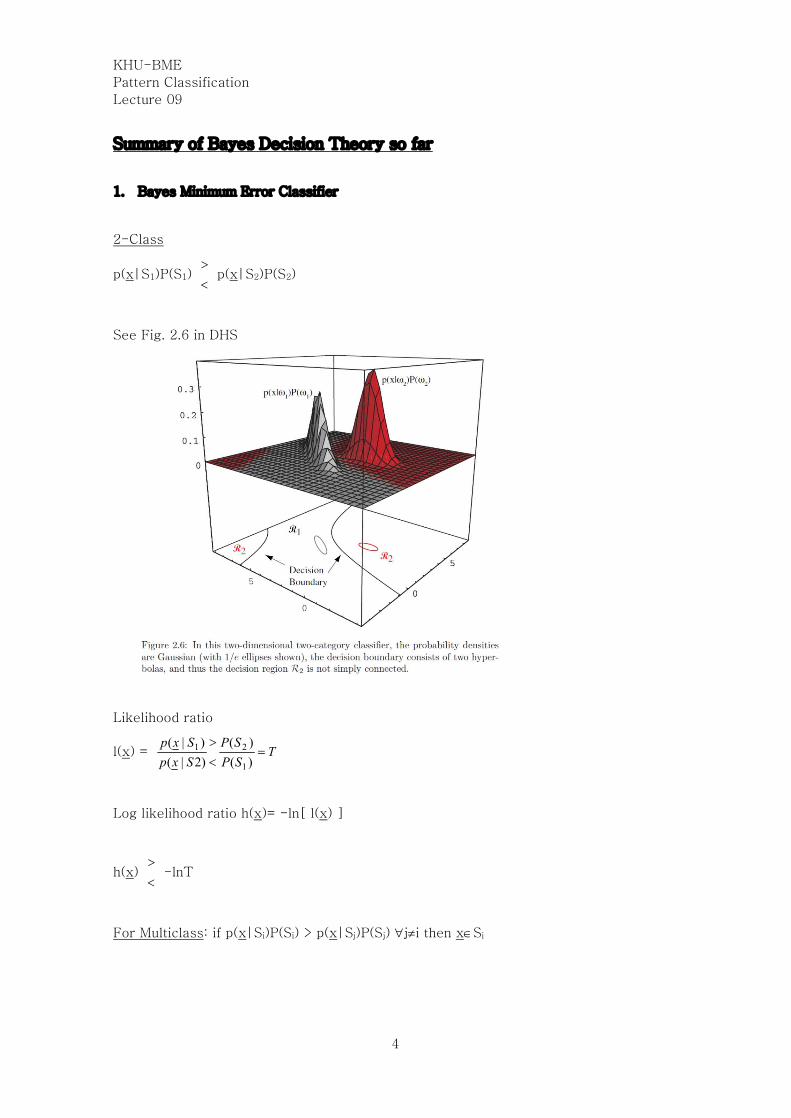
Summary of Bayes Decision Theory so far

1. Bayes Minimum Error Classifier

2-Class

p(x|S1)P(S1) <>

p(x|S2)P(S2)

See Fig. 2.6 in DHS

Likelihood ratio

l(x) = TSPSP

SxpSxp

=<>

)()(

)2|()|(

1

21

Log likelihood ratio h(x)= -ln[ l(x) ]

h(x) <>

-lnT

For Multiclass: if p(x|Si)P(Si) > p(x|Sj)P(Sj) "j¹i then xÎSi

KHU-BME


Lecture 09

5

2. Probability of Error Pe

2-class

Pe= òG2 p(x|S1) P(S1)dx + òG1 p(x|S2) P(S2)dx

For Multiclass

Pe=1- P{correct} <= This expression is much easier to understand.

P{correct}=åò=

G

K

iii xdSPSxp

i1)()|(

3. Bayes Minimum Risk Classifier

úúúú

û

ù

êêêê

ë

é

úúúú

û

ù

êêêê

ë

é

=

úúúú

û

ù

êêêê

ë

é

...

...)()|(.)()|(

...)|(

...)|(

22

11

21

1211

1

1

SPSxpSPSxp

C

CCC

xSR

xSR

kk

c

c

If Rc(Si|x)< Rc(Sj|x) for all j¹i => x Î Si or use gi(x)=-Rc(Si|x)

KHU-BME


Lecture 09

6

Classifiers (DHS 2.4)

Again, use a set of discriminant functions gi(x)

i.e., gi(x) > gj(x) for all j≠i.

Express gi(x) in terms of probabilites

gi(x)=p(Si|x)

gi(x)=p(x|Si)P(Si)

gi(x)=ln [p(x|Si)] + ln [P(Si)]

KHU-BME


Lecture 09

7

The Normal Density (DHS 2.5, p. 31)

- So far, general forms of density functions are considered

- Most widely studied density functions are the multivariate normal or

Gaussian density

- Why? Analytical tractability, most appropriate model

Univariate Density (DHS 2.5.1)

])(21exp[

21)( 2

sm

sp-

-=xxp

μ=expected value of x, average or mean

σ=standard deviation

Multivariate Density (DHS 2.5.2)

úûù

êëé -å--

å= - )()(

21exp

)2(1)( 1

2/12/mm

pxxxp T

d

μ=mean vector

å =covariance matrix

KHU-BME


Lecture 09

8

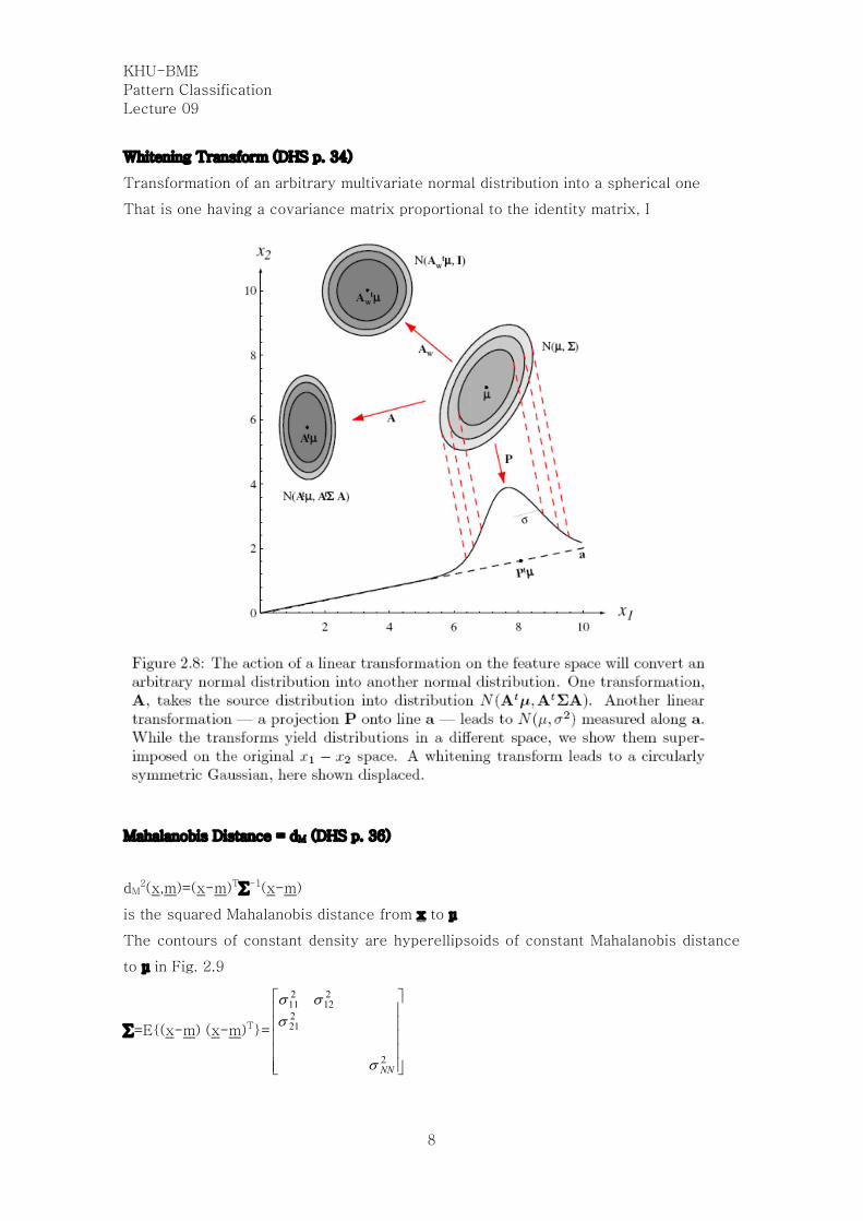
Whitening Transform (DHS p. 34)

Transformation of an arbitrary multivariate normal distribution into a spherical one

That is one having a covariance matrix proportional to the identity matrix, I

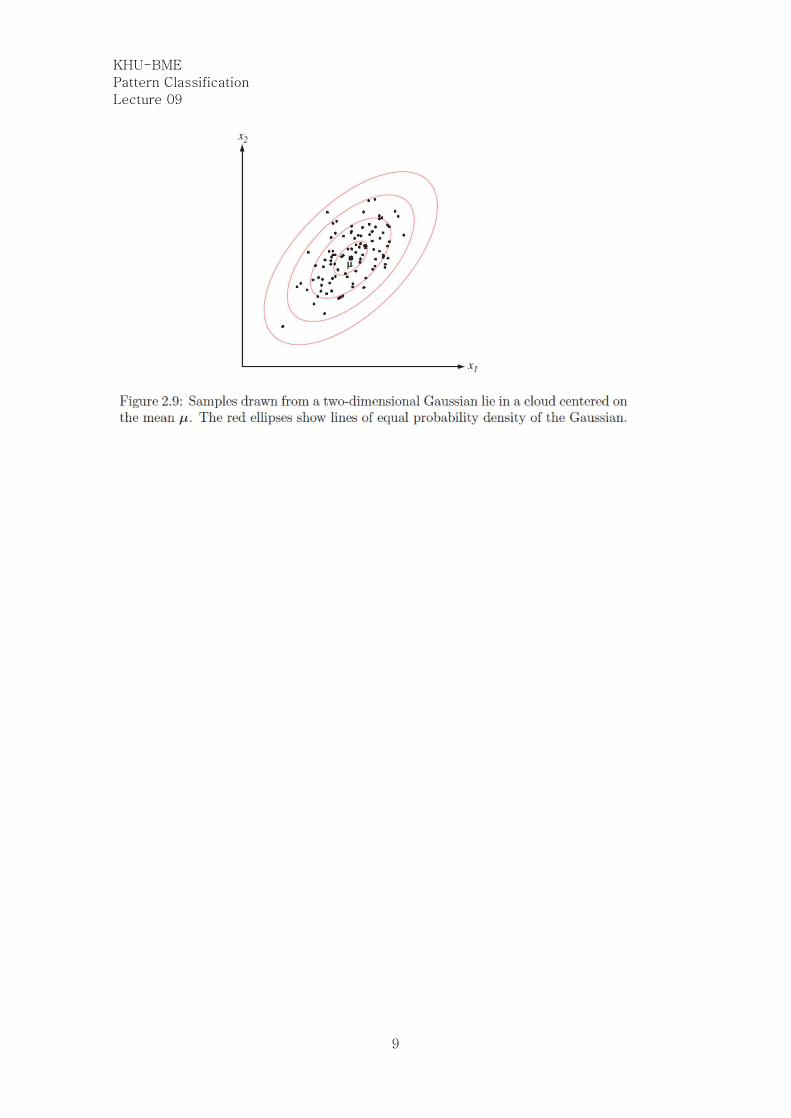
Mahalanobis Distance = dM (DHS p. 36)

dM2(x,m)=(x-m)Tå-1(x-m)

is the squared Mahalanobis distance from x to μ

The contours of constant density are hyperellipsoids of constant Mahalanobis distance

to μ in Fig. 2.9

å=E{(x-m) (x-m)T}=

úúúúú

û

ù

êêêêê

ë

é

2

221

212

211

NNs

sss

KHU-BME


Lecture 09

9

KHU-BME


Lecture 09

10

Discriminant Functions for the Normal Density (DHS 2.6, p. 36)

The minimum error rate classification can be done using the discriminant functions:

gi(x)=ln [p(x|Si)] + ln [P(Si)]

If p(x|Si)=N(μi,∑i)

)(lnln212ln

2)()(

21)( 1

iiiiT

ii SPdxxxg +S---S--= - pmm (DHS Eq. (49) p. 36)

Let’s examine this discrimination function and resulting classification for three special

cases.

Case 1: Same s (DHS 2.6.1)

If å=s2I=

úúúúú

û

ù

êêêêê

ë

é

2

2

2

...s

ss

å-1=(1/s2)I

dM2(x,m)=(1/s2)(x-m)T(x-m)= (1/s2) dE

2(x,m)

dE: Euclidean distance

)(ln2

)( 2

2

ii

i SPxg +-

-=s

μx

Since )()(2i

Tii μxμxμx --=-

)(ln]2[2

1)( 2 iiTi

Ti

Ti SPg ++--= μμxμxxx

s= 1++ n

Ti wxw

where ii μw 21s

= , )(ln2

121 ii

Tin SPw +-=+ μμ

s

This equation shows that squared distance 2

ix m- is normalized by the variance and

offset by lnP(Si). That is if x is equally near two different mean vectors, the optimal

decision favors the a priori more likely category.

KHU-BME


Lecture 09

11

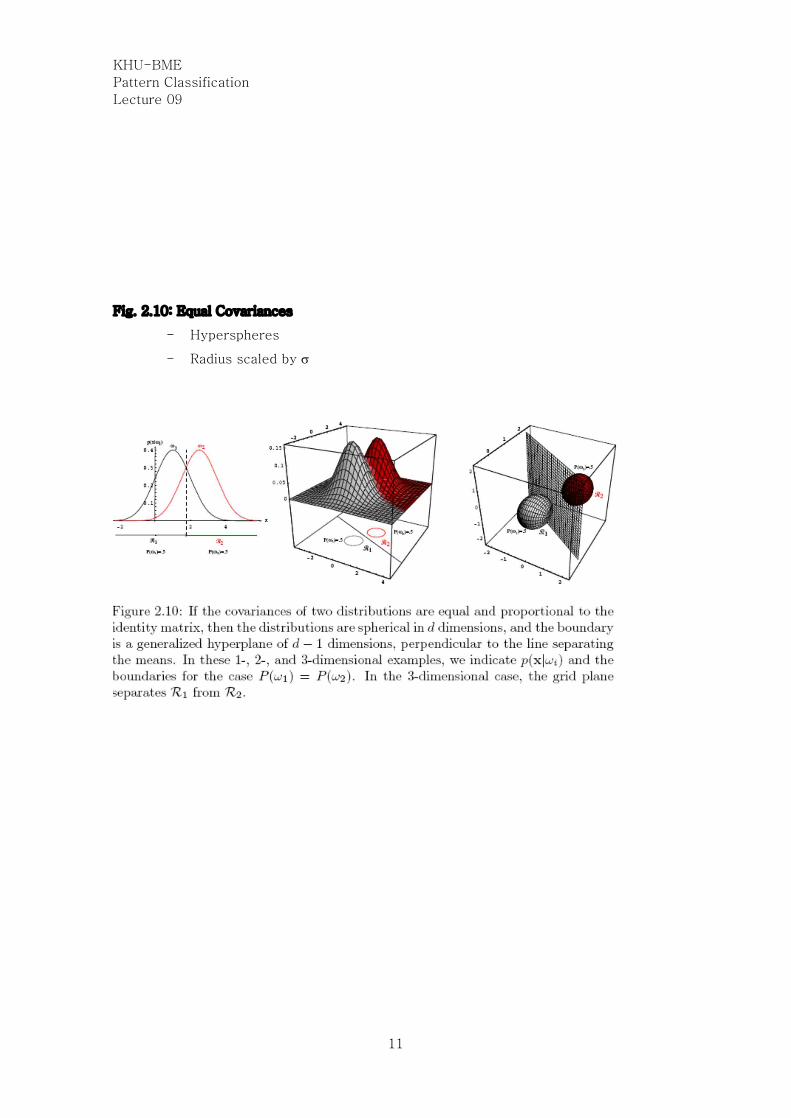
Fig. 2.10: Equal Covariances

- Hyperspheres

- Radius scaled by s

KHU-BME


Lecture 09

12

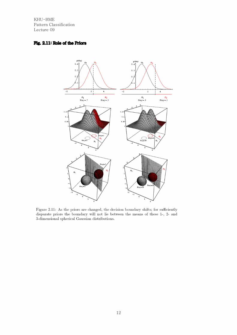
Fig. 2.11: Role of the Priors

KHU-BME


Lecture 09

13

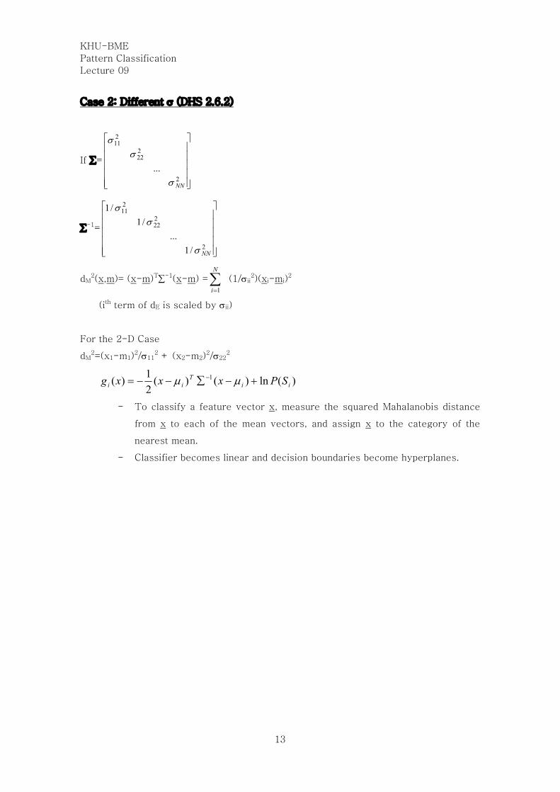
Case 2: Different s (DHS 2.6.2)

If å=

úúúúú

û

ù

êêêêê

ë

é

2

222

211

...

NNs

ss

å-1=

úúúúú

û

ù

êêêêê

ë

é

2

222

211

/1...

/1/1

NNs

ss

dM2(x,m)= (x-m)Tå-1(x-m) =å

=

N

i 1(1/sii

2)(xi-mi)2

(ith term of dE is scaled by sii)

For the 2-D Case

dM2=(x1-m1)

2/s112 + (x2-m2)

2/s222

)(ln)()(21)( 1

iiT

ii SPxxxg +-å--= - mm

- To classify a feature vector x, measure the squared Mahalanobis distance

from x to each of the mean vectors, and assign x to the category of the

nearest mean.

- Classifier becomes linear and decision boundaries become hyperplanes.

KHU-BME


Lecture 09

14

Fig. 2.12

- Hyperellipsoids

- Axes parallel to coordinate axes.

- Note the effect of priors.

KHU-BME


Lecture 09

15

Fig. 2.13

- No simple decision regions for Gaussians with unequal variance

KHU-BME


Lecture 09

16

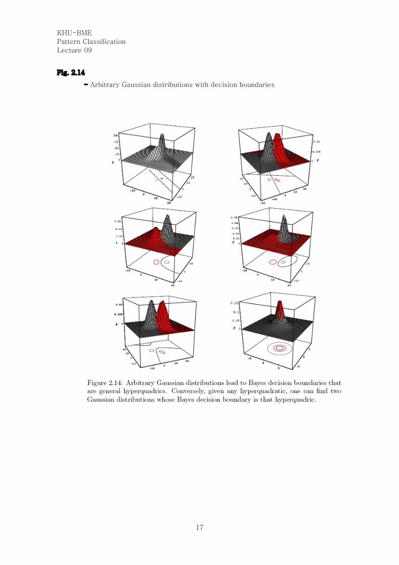
Case 3: If åi=general or arbitrary (DHS 2.6.3)

If the covariance matrices are different for each category, the resulting discriminant

functions are inherently quadratic

wxmxxxg iiiT

i +S+S-= -- 11

21)(

)(lnln21

21 1

iiiiTi SPmmw +S-S-= -

(DHS Eqs. (66)-(69))

å=

úúúúú

û

ù

êêêêê

ë

é

2

222

221

212

211

...

NNs

ssss

dM2(x,m)= (x-m)Tå-1(x-m)

apply orthonormal transformation (rotate basis)

x’=ETx

å’=ETåE=L=diagonal

ð hyperellipsoids (axes rotated)

2-D Case

2'22

222

2'11

2112 )()(

ss

mxmxdM-

+-

=

KHU-BME


Lecture 09

17

Fig. 2.14

- Arbitrary Gaussian distributions with decision boundaries

KHU-BME


Lecture 09

18

Fig. 2.15

- Arbitrary 3-D Gaussian distributions with decision boundaries

KHU-BME


Lecture 09

19

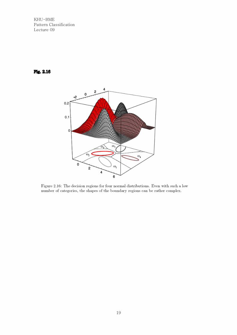
Fig. 2.16

bayes minimum error and minimum risk (multiple classes)web.khu.ac.kr/~tskim/patternclass lec note...

Documents