bayesian analysis of dynamic magnetic resonance breast images

2004 Royal Statistical Society 0035–9254/04/53475

Appl. Statist. (2004)53, Part 3, pp. 475–493

Bayesian analysis of dynamic magnetic resonancebreast images

Francesco de Pasquale,

Consiglio Nazionale delle Ricerche, Rome, Italy, and University of Plymouth, UK

Piero Barone and Giovanni Sebastiani

Consiglio Nazionale delle Ricerche, Rome, Italy

and Julian Stander

University of Plymouth, UK

[Received May 2002. Final revision September 2003]

Summary. We describe an integrated methodology for analysing dynamic magnetic resonanceimages of the breast. The problems that motivate this methodology arise from a collaborativestudy with a tumour institute. The methods are developed within the Bayesian framework andcomprise image restoration and classification steps. Two different approaches are proposedfor the restoration. Bayesian inference is performed by means of Markov chain Monte Carloalgorithms.We make use of a Metropolis algorithm with a specially chosen proposal distributionthat performs better than more commonly used proposals. The classification step is based ona few attribute images yielded by the restoration step that describe the essential features of thecontrast agent variation over time. Procedures for hyperparameter estimation are provided, somaking our method automatic. The results show the potential of the methodology to extractuseful information from acquired dynamic magnetic resonance imaging data about tumourmorphology and internal pathophysiological features.

Keywords: Bayesian methods; Classification; Dynamic magnetic resonance imaging;Hyperparameter estimation; Image analysis; Mammography; Restoration; Spatiotemporalmodels

1. Introduction

The aim of this collaboration between radiologists at the Istituto Regina Elena in Rome andstatisticians is to improve the diagnostic capabilities of the dynamicmagnetic resonance imaging(DMRI) technique for some breast pathologies. This task is important because breast canceris a serious public health problem and is the most common cancer in women (Heywang-Kobrunner and Beck, 1995). DMRI can offer considerable advantages over techniques such asX-ray mammography, ultrasonography, ‘transcutaneous’ core or needle biopsy and thermog-raphy (Highnam and Brady, 1999). It involves the acquisition of a temporal sequence of imagesof the breast acquired after the injection of a gadolinium salt contrast agent (Villringer et al.,1988). The contrast agent diffuses within the intravascular or interstitial spaces of tissue andmodifies the MR image intensities. Different breast tissues (normal, benign and malignanttumorous) show different patterns of uptake (Hayton et al., 1999). In particular, DMRI signals

Address for correspondence: Francesco de Pasquale, Department of Mathematics and Statistics, University ofPlymouth, Drake Circus, Plymouth, Devon, PL4 8AA, UK.E-mail: [email protected]

476 F. de Pasquale, P. Barone, G. Sebastiani and J. Stander

Fig. 1. Typical time patterns for DMRI intensity for a breast tissue pixel: the curve showing a clear maximumis often associated with malignant lesions; the other two curves are mostly associated with benign lesions;one time unit is 15 s and the signal time course is reported in arbitrary units

within malignancies are especially sensitive to the contrast agent owing to the increased vas-cularity, permeability and interstitial space that are associated with these conditions. In Fig. 1some typical contrast agent uptakes are shown. Important features of these patterns are thespeed of the initial variation in intensity, or wash-in, and the presence or absence of a finaldecrease, or wash-out.In general, the morphology of a lesion represents important information for classifying

tumours. The presence of an internal structure may also be diagnostically useful. Accordingly,the main aims of DMRI data analysis are to identify the lesion, to highlight its morphologyand to investigate its structure. Unfortunately, distortions affecting the data make these tasksdifficult.There has been much research about the analysis of DMRI data. Important references are

Kuhl et al. (1999), Mussurakis et al. (1997, 1998) and Gribbestad et al. (1992), although theseresearchers made no attempts to remove either deterministic distortions due to movement ofpatients or random distortions due to experiment imperfections. Hayton et al. (1999) andKrishnan et al. (1999) presented methodology to correct for motion of the breast, whereasHayton et al. (1996) used a pharmacokinetic model for the acquired signals to localize tumours.The ‘three time point method’ of Weinstein et al. (1999) uses three images of the sequence toidentify certain pathophysiological features.In all these methods either image pixels are analysed independently or no image restoration

procedure is developed. In contrast, in this paper we discuss in detail two approaches that arebased on spatiotemporal models. In one of these we use a specific parametric temporal modelfor the evolution of image intensity at each pixel. Accordingly, we refer to our methods as ‘para-metric’ and ‘nonparametric’. Of course from a statistical point of view the overall methodologyis parametric in both cases.Ourmethods yield attributes that succinctly describe the intensity pattern at each pixel. These

are then used in a classification step to reveal the structure of the tumour. Our algorithms forspatiotemporal restoration have been developedwithin the Bayesian framework (Winkler, 1995;Geman and Geman, 1984). The basic ingredients of the framework are the data model P.y|x/and the prior distributionP.x/, both of whichmay depend on unknown parameters. The formerprovides a description of the observed data y given an underlying, unobserved image sequencex. The latter is a probabilistic model for our ‘a priori’ beliefs about the image sequence x. These

Dynamic Magnetic Resonance Breast Images 477

ingredients are combined by using Bayes theorem to form the posterior distribution

P.x|y/∝P.y|x/ P.x/of the image sequence given the data. Our methods are automatic, as we provide techniquesfor estimating the hyperparameters of the prior distribution. Inference is performed by sam-pling from the posterior distributionP.x|y/ usingMarkov chainMonte Carlo algorithms (Gilkset al., 1996). In particular, we use theMetropolis algorithm (Metropolis et al., 1953) with a spe-cially chosen proposal distribution that performs better than more commonly used proposals.We often experienced advantages when using the Bayesian approach. In fact, the specific priorinformation that is adopted compensates the poor quality and the limited amount of data cor-responding to the tumorous region with the result that distortions that occur with pixel-by-pixelanalysis are reduced. The Bayesian approach also allows the quantification of uncertainty inthe estimates. To reduce the quantity of results that we present we do not include any of thecomparisons that we performed with existing approaches such as wavelet-based methods.In this paperwe consider a typicalDMRI sequence of 20 two-dimensional images of 256× 256

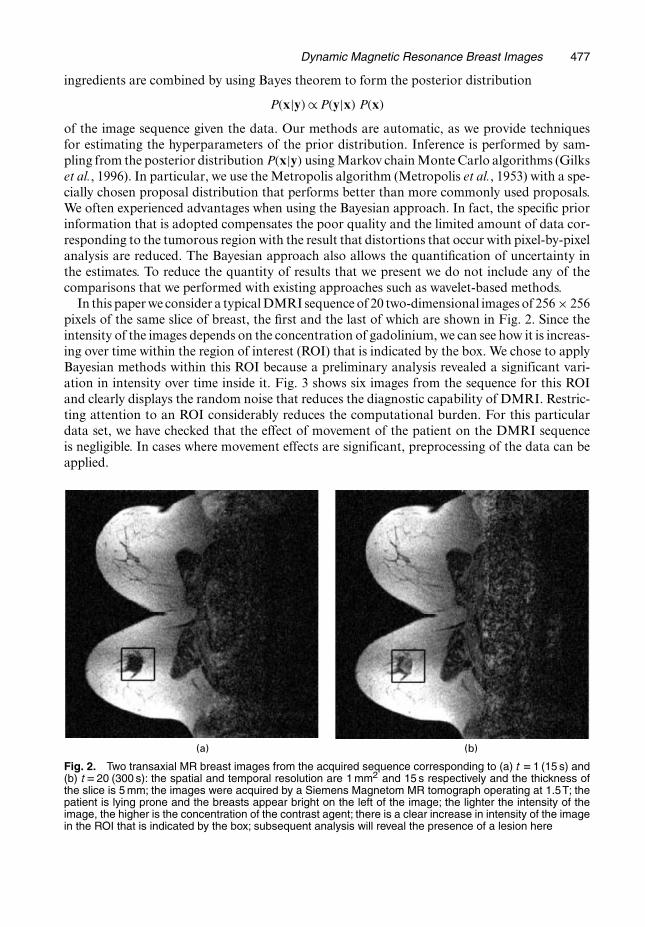
pixels of the same slice of breast, the first and the last of which are shown in Fig. 2. Since theintensity of the images depends on the concentration of gadolinium, we can see how it is increas-ing over time within the region of interest (ROI) that is indicated by the box. We chose to applyBayesian methods within this ROI because a preliminary analysis revealed a significant vari-ation in intensity over time inside it. Fig. 3 shows six images from the sequence for this ROIand clearly displays the random noise that reduces the diagnostic capability of DMRI. Restric-ting attention to an ROI considerably reduces the computational burden. For this particulardata set, we have checked that the effect of movement of the patient on the DMRI sequenceis negligible. In cases where movement effects are significant, preprocessing of the data can beapplied.

(a) (b)

Fig. 2. Two transaxial MR breast images from the acquired sequence corresponding to (a) t D 1 (15 s) and(b) tD 20 (300 s): the spatial and temporal resolution are 1 mm2 and 15 s respectively and the thickness ofthe slice is 5 mm; the images were acquired by a Siemens Magnetom MR tomograph operating at 1.5T; thepatient is lying prone and the breasts appear bright on the left of the image; the lighter the intensity of theimage, the higher is the concentration of the contrast agent; there is a clear increase in intensity of the imagein the ROI that is indicated by the box; subsequent analysis will reveal the presence of a lesion here


(a) (b) (c)

(d) (e) (f)

Fig. 3. Six images from the DMRI sequence restricted to the ROI in Fig. 2 acquired at times (a) t D 1,(b) t D2, (c) t D3, (d) t D5, (e) t D10 and (f) t D20, where one time unit is 15 s

The remainder of this paper is organized as follows. In Sections 2 and 3 we present our non-parametric and parametric approaches to image restoration. We also develop novel solutionsto the problem of estimating the model hyperparameters. In Section 4 the classification proce-dure is described. Results obtained by using the proposed methodology are given in Section 5.Finally, in Section 6 we present a brief discussion and our conclusions.

2. Nonparametric approach

In the nonparametric approach, Bayesian estimation of the true intensities of the images isperformed at each pixel of a selected ROI such as that shown in Fig. 3.This is donewithout using a parametric temporalmodel for the evolution of the image’s inten-

sity. From the estimated images relevant quantities describing the variation in intensity over timeat each pixel are computed. We later use these quantities to classify the pixels of the ROI into agiven number of classes. Following the Bayesian paradigm, we shall introduce the image datamodel, the prior model and the adopted estimator based on the posterior distribution.

2.1. Image data modelLet yi={yi.1/, . . . ,yi.T/} represent the observed temporal intensity profile at pixel i of the ROI,where i=1, . . . ,n, and let y = .y1, . . . ,yn/ be all the observed data, i.e. a sequence of T images.In the initial image of the sequence, namely y1, changes in intensity appear for the first time


due to the arrival of the contrast agent. Our values of n and T are 33× 33 and 20 respectively.Similarly, let x = .x1, . . . ,xn/ be the true, but unobserved, image sequence to be estimated.Since we assume that the deterministic degradation due to motion of the patient is negligible,

the acquired image sequence y will be related to x by

yi.t/=xi.t/+ "i.t/, i=1, . . . ,n, t=1, . . . ,T , .1/

where the errors "i.t/ are assumed to be independently distributed. We take the time unit to bethe time interval between two contiguous images, namely 15 s. For anMR image the distributionof "i.t/ is known to be a Rice distribution (Henkelman, 1985; Sijbers et al., 1999). It follows thatfor DMRI the distribution of y given x is

P.y|x/=n∏i=1

T∏t=1

yi.t/

σ2exp

[− {yi.t/−xi.t/}2

2σ2

]I0

{yi.t/ xi.t/

σ2

},

where I0 is the modified Bessel function of the first kind. If the expected value of the acquiredimage intensities is much larger than σ, we can approximate this Rice distribution by aGaussiandistribution with variance σ2. In the background region of the image this distribution becomesa Rayleigh distribution with variance .2−π=2/σ2. We use this property to estimate σ2 on thebasis of the acquired image intensity in the background region. We perform estimation of x onthe basis of bothRice andGaussian distributions. As only very small differences in the estimatesare obtained, we prefer to use the Gaussian distribution for computational simplicity.

2.2. Prior modelOur a priori distribution for the true image sequencemust be able tomodel both the continuity ofthe temporal evolution at each spatial location and the presence of homogeneous spatial regionswithin every image of the sequence. To achieve this we relate stochastically in a separate waythe differences between image intensities at contiguous times at each pixel and the differencesbetween neighbouring pixels in space at each time. We do this through the following factorizedMarkov random-field model:

P.x/∝T∏t=1

exp[−βs

∑<ij>

Vs{xi.t/−xj.t/}] n∏i=1

exp[−βt

∑<t′t′′>

Vt{xi.t′/−xi.t′′/}], .2/

where Vl is the prior potential in space or time, l∈{s, t},<ij> indicates second-order neighbourpixels in space, <t′t′′> indicates first-order neighbour pixels in time and βl is the smoothinghyperparameter in space or time, l∈{s, t}.The neighbours of pixels belonging to the border of the ROI are only those that are included

in the ROI. A similar choice is adopted for the borders of the time interval. The prior distribu-tion (2) is a pairwise interaction model that is characterized by the prior potentials Vs and Vt .In particular, we took

Vl.z/=− log{pl.z/}, .3/

where pl is the distribution of grey level differences in x (Sebastiani and Godtliebsen, 1997). Wemodelled pl.z/ by using a Cauchy density as

pl.z/∝{1+

(z

δl

)2 }−1

, .4/

where δl, l∈{s, t}, are two further hyperparameters to be estimated. The meaning of δl will bediscussed in Section 2.4. With this choice we have


Vl.z/= log{1+

(z

δl

)2 }: .5/

Model (5) penalizes differences depending on their amplitude compared with the parameterδl. Other choices for Vl have been proposed with similar behaviour (Kunsch, 1994). The keyfeature of the approach is to define Vl through pl by equation (3), as this allows us to propose asuccessful procedure for estimating δl. Among the various models that we tried for pl.z/, model(4) leads to the most reliable hyperparameter estimation results.

2.3. EstimationIn the Bayesian approach, different estimators can be adopted such as the mean value of xunder the posterior distribution P.x|y/, MMSE, or the image that maximizes P.x|y/, MAP.WechoseMMSE because it is more stable thanMAP (Marroquin et al., 1987) and can be obtainedwithout solving an optimization problem.Using Bayes theoremwe haveP.x|y/∝P.y|x/P.x/where the associated normalizing constant

is unknown. Because MMSE is not available in closed form we use Markov chain Monte Carlosimulations to obtain a good approximation x to it (Gilks et al., 1996). In particular, we use theMetropolis algorithm (Metropolis et al., 1953). This algorithm starts from an arbitrary initialpoint and iteratively moves from state x to state x′ in two steps. In the first step a candidate pointx′ is generated from a proposal distributionQ.x →x′/. Next x′ is accepted with probability

min{1,P.x′|y/Q.x′ →x/P.x|y/Q.x →x′/

}:

In our case the candidate state x′ differs from the current state in at most one component xi.t/and we update the whole of x by using a fixed systematic schedule. The distributionQ is takento be normal with expected value yi.t/ and variance σ2; see Section 5.1.1 for further discussion.We take x to be the mean of the last half of the Markov chain sequence of images, the length ofwhich is determined by monitoring the spatial mean. In our method we begin by estimating allthe hyperparameters automatically as we shall now discuss.

2.4. Hyperparameter estimationAll the hyperparameters .βs,βt , δs, δt/ play an important role in our procedure. The parametersβs and βt represent the weights of the spatial and temporal prior potentials with respect tothe image data model potential. Inappropriate values of these parameters can lead to eitheroversmoothed or noisy estimated images. The parameters δs and δt are also very importantbecause they control the amplitude of the discontinuities that will be preserved in the estimatedimages.We begin by estimating δs and δt . Our estimation procedure is based on minimizing the dif-

ference between pl.∆yl/, the empirical distribution of observed image intensity differences, andthe associated theoretical pl.∆yl/, where∆yl represents all the spatial or temporal intensity dif-ferences in neighbouring pixels of the observed sequence y (Sebastiani and Godtliebsen, 1997).From equation (1) we obtain that ∆yl=∆xl+∆"l, from which it follows that

pl.∆yl/=pl.∆xl/⊗pl.∆"l/ .6/

where⊗ indicates the convolution integral. From the Gaussian noise distribution it follows thatpl.∆"l/ is an N.0, 2σ2/ distribution. On the basis of pl.∆xl/ from expression (4) and pl.∆"l/,


pl.∆yl/ can be computed by performing the convolution (6) numerically. We now minimize thesum of the absolute values of the differences between pl.∆yl/ and pl.∆yl/ over parameter δlin a finite set of suitable values. To calculate this difference we compute pl at the same finiteset of values for which pl is defined. Once δs and δt have been found, we estimate βs and βt byminimizing the discrepancy between a theoreticalχ2

T -distribution and the empirical distributionof the values in the set:

ΣI ={T∑t=1

{yi.t/− xi.t;βs,βt/}2σ2

, i∈I}:

Here I is a set of pixels in the ROI where significant differences in the intensity of the image intime are present and xi.t;βs,βt/ is the estimated image at pixels in I corresponding to a givenchoice of βs and βt . We identify the region I before the Bayesian analysis has been performed bya one-tailed hypothesis test based on the estimated distribution of the mean variation in inten-sity of the image in time within a non-tumorous region selected manually by the radiologist.The distance between the empirical distribution of the values in ΣI and the χ2

T -distributiondecreases as xi.t;βs,βt/ becomes closer to xi.t/.

3. Parametric approach

Alternatively, we may adopt a parametric temporal model for the true image intensity profile ateach pixel. Themodel parameters are estimated by the Bayesian approach and some of them areused as attributes for the subsequent classification procedure. We now discuss the image datamodel, the prior model and the estimator adopted.

3.1. Image data modelWe assume that xi.t/ takes the functional form xi.t/=fθi .t/, where the temporal model fθi .t/ isgiven by

fθi .t/=

Ii+ Mi− Ii

1− exp{−∆.pi−1/=τi} [1− exp{−∆.t−1/=τi}] 1� t�pi,

Mi−Mi−FiT −pi .t−pi/ pi� t�T ,

in which θi= .Ii,Mi,Fi,pi, τi/ represents the parameter vector for pixel i, θ = .θ1, . . . , θn/ is thesequence of parameter vectors for the n pixels and∆=15 s is the temporal interval between twosubsequent images so that the units of τi are seconds. These parameters are illustrated in Fig. 4.Combining the parametric model with the Gaussian noise distribution we obtain the followingimage data model:

P.y|θ/= 1.2πσ2/nT=2

n∏i=1

T∏t=1

exp[

− {yi.t/−fθi .t/}22σ2

]:

3.2. Prior modelThe a priori model that is used here is similar to that adopted for the nonparametric approach.In fact, for each parameter we take into account both continuity and the presence of differ-ent structures in the image. Furthermore, we assume that the parameters are not independent.Among the different types of dependent models with which we experimented, the one thatperforms best is

P.θ/=PI,M,F .I,M,F/ Pp,τ .p, τ /


Time

Sig

nal T

ime

Cou

rse

(a.u

.)

A B

•

•

•

•• •

••••••••••••••

1 5 10 15 20p

0

500

1000

1500

2000

2200

I

F

M

τ = 60

τ = 15

Fig. 4. Meaning of the parameters θ D .I , M, F , p, τ / of the parametric temporal model and the area attri-butes A and B from the nonparametric approach: two parametric time patterns are shown—θ D .200,1400, 900, 6:5, 15/ ( ) and θ D .200, 1400, 900, 6:5, 60/ (– – – )—and the curves coincide after p (�, timepoints t D1, . . . , 20 where one time unit is 15 s) (the units of τ are seconds)

where

PI,M,F .I,M,F/∝ exp[

−β1∑<ij>

log{1+

(Ii− Ij

δI

)2

+(Mi−Mj

δM

)2

+(Fi−Fj

δF

)2 }]

Pp,τ .p, τ /∝ exp[

−β2∑<ij>

log{1+

(pi−pj

δp

)2

+(

τi− τj

δτ

)2 }] .7/

where <ij> indicates second-order neighbours in space and β1, β2, δI , δM , δF , δp and δτ arethe hyperparameters.

3.3. EstimationAgain we adopt MMSE for θ. An approximation of this is obtained by using the Metropolisalgorithm with uniform proposals. The ranges of the parameters for the uniform proposals aredefined as follows. The ranges for I and F are the same as those of y1 and yT respectively. Therange for M corresponds to the minimum and maximum values of the whole measured imagedata whereas the range for p is [2,T −2]. The range for τ is∆[0:2,T=3]. MMSE is approximated


as the mean of the last half of the Markov chain sequence of images, the length of which isdetermined by monitoring the spatial mean of the parameters.

3.4. Hyperparameter estimationIn expression (7) the hyperparameters are .β1,β2, δI , δM , δF , δp, δτ /. To estimate δI and δF weuse the procedure that was described in Section 2.4 by considering the empirical distributionof the pixelwise differences of yi.1/ and yi.T/. For δM , δp and δτ , we estimateM, p and τ withβ1 =β2 =0. The values of these three parameters are then set to the standard deviation of theempirical distribution of the pixelwise differences for these images (Glad and Sebastiani, 1995).We cannot use the procedure that was described in Section 2.4 because the relationship betweenM, p and τ and the image sequence that is observed does not follow a simple additive model.For the hyperparameters β1 and β2 we follow the approach that was described in Section 2.4.

4. Classification

Afterperformingnonparametric orparametric restoration,weproceedwith classificationwithinthe ROI by using a recent method due to Sebastiani and Sørbye (2002). The procedure is basedon a few attributes describing the relevant features of the image intensity time pattern for eachpixel. From the nonparametric approach, we use the areas A and B that are shown in Fig. 4as these quantify gadoliniumwash-in andwash-out and are easily calculated from the smoothedtemporal pattern. From the parametric approach we use the parameters τ and M − F ,as these also quantify gadolinium wash-in or wash-out. For comparable values of M − I, Adecreases with τ . However, although we could calculate A from the estimated temporal model,doing so would result in less spatial regularity than using τ for which we adopted a spatialprior model. Let di= .d1,i, . . . ,dm,i/ be a vector containing the m attributes at pixel i. In ourcase we takem=2. The classification procedure can be represented by a mapping of every pixeli to a class ki ∈{1, 2, . . . ,K} where K is the number of classes that are considered. The valueof K can be chosen by the radiologist. We could take K=3, corresponding to normal, benignand malignant tumorous tissues. Alternatively, the classification can be performed only in atumorous region I predetermined by the test mentioned in Section 2.4. In this case we wouldset K=2, corresponding to benign and malignant tumorous tissues.

4.1. Attribute modelThe jth attribute for the kth class is assumed to follow a Gaussian distribution with expectedvalue cj,k and variance Vj,k. The attributes are assumed to be conditionally independent withthe result that the distribution of d = .d1, . . . ,dn/ given the classification vector k = .k1, . . . , kn/ is

p.d|k, c,V/=n∏i=1

m∏j=1.2πVj,ki /

−1=2 exp{−.dj,i− cj,ki /2=2Vj,ki},

where c = .c1, . . . , cK/ and V = .V1, . . . ,VK/, in which ck= .c1,k, . . . , cm,k/ and Vk=.V1,k, . . . ,Vm,k/ are the attribute means and variances for tissue class k. These vectors areassumed to be unknown and will be estimated at the same time as k.

4.2. Prior modelOur prior assumption about the classified image is that neighbouring pixels are more likely tobelong to the same class than to different classes. Hence we adopt the Potts model (Potts, 1952):


P.k|β/= 1Zβ

exp.−βUk/= 1Zβ

exp(β

∑<ij>

δki,kj

),

where the hyperparameter β must be estimated and Zβ is the unknown normalizing factor.

4.3. EstimationInference about k, c, V and β is based on their joint posterior distribution. By using Bayestheorem and the assumptions that P.d|k, c,V,β/=P.d|k, c,V/ and that P.k|β, c,V/=P.k|β/,we obtain

P.k, c,V,β|d/∝P.d|k, c,V/P.k|β/ P.c,V,β/,where P.c,V,β/ is the prior distribution on c, V and β. Here we assume a uniform prior ina suitable range for these parameters. As we now adopt a fully Bayesian approach (Besag,1989) we need to estimate Zβ up to a proportionality constant for a range of values of β.Since

Zβ =∑kexp.−βUk/,

exact calculation is not feasible owing to the high numberKn of configurations that are involved.However, we proceed by noting that

@ log.Zβ/

@β= 1Zβ

@Zβ

@β=−∑

k

1ZβUk exp.−βUk/=−EP.k|β/.Uk/, .8/

where EP.k|β/.Uk/ is the expected value of the energy function Uk under P.k|β/. Next we inte-grate equation (8) with respect to β to obtain

log.Zβ/− log.Zβ0/=−∫ β

β0

EP.k|β′/.Uk/ dβ′,

for some fixed value β0. We approximate EP.k|β′/.Uk/ by using the Metropolis algorithm fora finite number of values of β and calculate the integral numerically by using Simpson’s rule.Related approaches for approximating the normalizing constant can be found in Gelman andMeng (1998) and Green and Richardson (2002).The estimator that is chosen is the classification image corresponding to the maximum of the

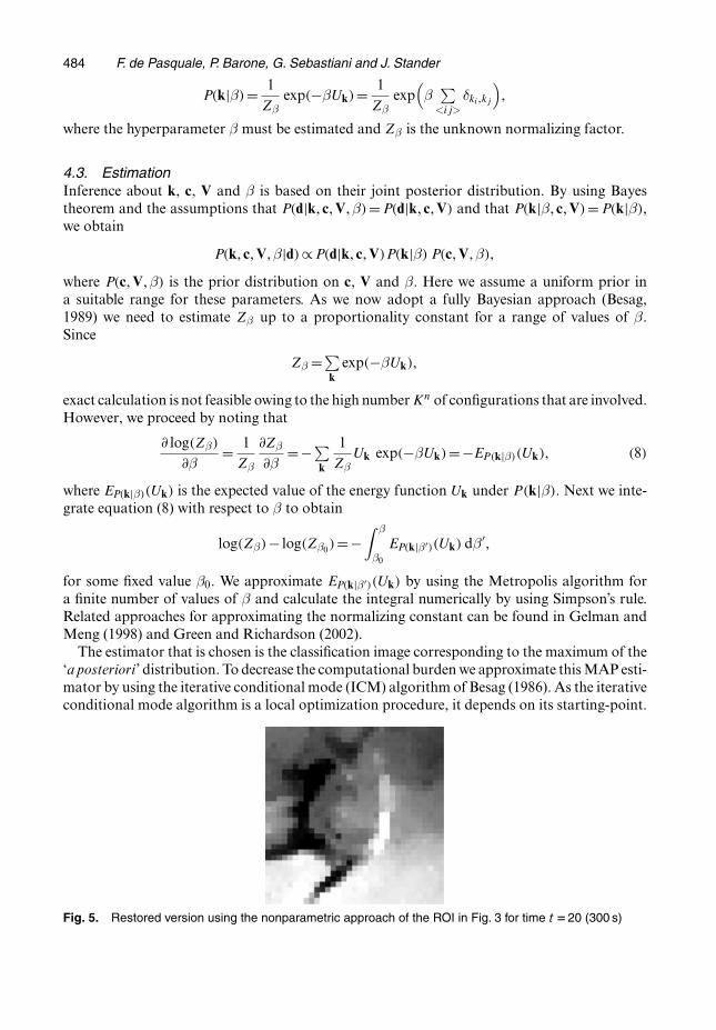
‘a posteriori’ distribution. To decrease the computational burdenwe approximate thisMAP esti-mator by using the iterative conditional mode (ICM) algorithm of Besag (1986). As the iterativeconditional mode algorithm is a local optimization procedure, it depends on its starting-point.

Fig. 5. Restored version using the nonparametric approach of the ROI in Fig. 3 for time t D20 (300 s)


–1500 –1000 –500 0 500 1000 15000

0.5

1

1.5

2

2.5

3

3.5x 10–3

Intensity differences (a.u.)

Per

cent

age

Time

Space

(a)

(b)

Fig. 6. Hyperparameter estimation: (a) comparison between pl.∆yl / for the optimal δl ( ) and theempirical distribution pl .∆yl / ( . . . . . . .) for both space and time and (b) comparison between the theoreticalχ2

T -density ( ) and the empirical distribution of ΣI for the optimal βs and βt ( ) for a possible tumorousregion I


We chose the k-means clustering algorithm (see Glasbey and Horgan (1995)) output as thestarting-point. The initial point for the k-means clustering algorithm is a classification imagebased on the modes of the histogram of one of the class attributes; see Sebastiani and Sørbye(2002) for further details.

(a) (b)

Fig. 7. Images of the attributes (a) A and (b) B from the nonparametric approach in I

0 50 100 150 200 250 300 350 4000

10

20

30

40

50

60

70

80

90

RMSE

No. of iterations

Fig. 8. Comparison between Metropolis algorithms with different proposals: Gaussian independence pro-posal with measured pixel image intensity as the proposal mean and σ2 as the proposal variance ( ),optimal Gaussian random walk (– – – –) and uniform independence proposal ( . . . . . . .) (each iteration on thehorizontal axis corresponds to a full update of the ROI; the vertical axis represents the root-mean-squarederror between the true image and the current estimate of the posterior mean)


5. Results

In Sections 5.1 and 5.2 we illustrate some of the results that were obtained from our nonpara-metric and parametric approach to image restoration. In Section 5.3 classification results arepresented.

5.1. Nonparametric approachIn Fig. 5 we show the restoration from the nonparametric approach for the ROI that is shown inFig. 3 for time t=20. We note that random variations have been reduced compared with Fig. 3,and the edges of the underlying structure have been preserved, so maintaining informationabout the tumour’s morphology. To assess the effectiveness of the procedures for hyperparam-eter estimation we show in Fig. 6(a) a comparison between pl.∆yl/ for the optimal δl and theempirical distribution pl.∆yl/ for both space and time. The agreement is very good. In Fig. 6(b)we present a comparison between the theoretical χ2

T -distribution and the empirical distributionof ΣI for the optimal βs and βt . Again, the agreement is good.The attributes A and B for I are shown in Fig. 7. Structures resembling a ‘C’ and a ‘U’

appear in Fig. 7. Although these structures are not clearly outlined, the information in theA- and B-images will lead the classification procedure towards a meaningful structure as weshall see in Section 5.3.

5.1.1. A new proposal for the Metropolis algorithmTo obtain x we use an ad hoc version of the Metropolis algorithm (Metropolis et al., 1953)with a proposal function based on the data distribution. In particular we use a Gaussian inde-pendence proposal with measured pixel image intensity as the proposal mean and σ2 as theproposal variance. We performed a simulation study to compare this proposal function withother choices, such as a uniform independence proposal and a random walk with Gaussianproposal optimized with respect to the variance. We took a real MRI image with very low noiseand restored a noisy version of it. The root-mean-square error between the true image and thecurrent approximation of the posterior mean is plotted as a function of Markov chain Monte

(a) (b)

Fig. 9. Images of the attributes (a) τ and (b) M �F from the parametric approach


0 2 4 6 8 10 12 14 16 18 200

200

400

600

800

1000

1200

1400

1600

1800

2000

2200

Sig

nal T

ime

Cou

rse

(a.u

.)

Time

0 2 4 6 8 10 12 14 16 18 200

200

400

600

800

1000

1200

1400

1600

1800

2000

2200

Sig

nal T

ime

Cou

rse

(a.u

.)

Time

(a)

(b)

Fig. 10. Comparisons between the acquired image intensity time profiles (–�–) and the restored profilefrom the nonparametric (– – – ) and the parametric ( ) approach: the profiles in (a) and (b) correspondto different pixels; one time unit is 15 s


Carlo iteration number in Fig. 8 for our proposal function and the two others mentioned above.Our proposed algorithm reaches convergence much earlier than the other two algorithms. Weobserve the same behaviour for different levels of noise and for other kinds of original images.

5.2. Parametric approachIn Fig. 9 we show our estimates of τ andM−F . The structures in Fig. 7 are more evident here.To assess the validity of the parametric approach and to compare it with the nonparametricapproach, we consider the time patterns from the acquired and restored images at two differentpixels within I. Fig. 10(a) shows an example where the parametric approach provides a betterfit than the nonparametric approach. This occurs in most of the pixels within the tumorousregion and may lead us to prefer the parametric model. In Fig. 10(b) a different situation is pre-sented. Here the data provide evidence for a time pattern of a different kind from that allowedby the parametric model. In cases like this the parametric model seems too rigid and unable todescribe the true time evolution properly. Overall, our choice of method can be based on theinterpretation of classification results by radiologists.In contrast with other methods, the Bayesian approach provides us with both point estimates

and credibility intervals for the parameters. This may be useful in further steps of the analysis,such as interpatient surveys. As an example, in Fig. 11 we present MMSE and its associated95% credibility intervals for a central row of the parameter τ that is shown in Fig. 9(a).

5.3. ClassificationWithin region I that is now shown in Fig. 12(a), we consider two classes corresponding tobenign and malignant tumorous tissues. In Fig. 12(b) we show the classification results based

10

60

50

40

30

20

10

015

Pixel number

20 25

τ (s

ec.)

Fig. 11. Point estimates and 95% credibility intervals for a central row of the parameter τ that is shown inFig. 9(a)


(a) (b)

(c)

Fig. 12. Tumour localization and classification: (a) tumorous region I that was identified by the hypothesistest described in Section 2.4 (white) is superimposed on the breast; (b) classification result for the attributesfrom the nonparametric approach; (c) classification result for the attributes from the parametric approach

on the attributes A and B that were obtained from the nonparametric approach. We note a ringstructure that is frequently present in these kinds of tumour (Heywang-Kobrunner and Beck,1995). Radiologists have advised us that this structure is consistent with a necrotic region atthe centre of the tumour caused by the tumorous growth mechanism. In Fig. 12(c) we showthe classification based on the attributes τ and M−F that was obtained from the parametricapproach. Very similar results were achieved by using the parameters p and M−F . We noteagain the ring structure. Finally, in Fig. 13 we show the average time patterns that were cal-culated in the two subregions of the tumour shown in Fig. 12(b). We observe different timepatterns of image intensity. Almost identical curves are obtained from the classification that is


0 2 4 6 8 10 12 14 16 18 200

200

400

600

800

1000

1200

1400

1600

1800

2000

2200

Time

Sig

nal T

ime

Cou

rse

(a.u

.)

Fig. 13. Average signal time course estimated by the nonparametric approach in the black ( ) andwhite (� – � – �) regions of Fig. 12(b): one time unit is 15 s

presented in Fig. 12(c). These time courses resemble the commonly observed behaviour that isillustrated in Fig. 1. These results show the success of the whole procedure for investigating theinternal structures of the lesion.

6. Discussion and conclusions

In this paper we have presented a novel Bayesian methodology for the analysis of DMRI ofthe breast. In the methodology proposed, we perform first a restoration step. The estimatedquantities at different locations are made to depend on each other to take into account thelocal regularity features of the tumour. A further step will consist of modelling global informa-tion about the boundary shapes of tumours. Medical experience shows that this information isrelevant for characterizing lesions.By comparing the attribute images from the parametric and the nonparametric approaches,

we observe that the former present a lower degree of random distortion. Two explanations forthis are possible. First, in the nonparametric method there are four times as many parameters asin the parametric approach. Secondly, in the parametric method the attributes are either param-eters on which the prior distribution is directly defined or a simple function of them, whereasin the nonparametric approach the prior distribution is defined on the true image intensityvariables and the attributes are calculated pixel by pixel from estimates of these.After calculating the attributes, the analysis proceeds by classifying image pixels into a few

classes. This number is predetermined from the radiologist’s experience and needs. The classescorresponding to typical DMRI time patterns are normal, benign and malignant tumoroustissues. The classification can be obtained in two different ways. In one of them, each of the


pixels in the ROI is classified as one of the above three types of tissue. In the other, a tumorousregion I is identified by a hypothesis test and each of its pixels is classified as either benignor malignant. The results that are obtained from these two approaches seem to contain thesame qualitative information, such as the presence of a ring structure. However, the approachconsidering only pixels within I seems to produce more robust results with a lower degree ofrandom variations.Apart from the initial choice of a non-tumorous region and of the ROI, the whole meth-

odology is fully automatic. To achieve this we developed methodology for hyperparameterestimation. We also proposed a modified Metropolis algorithm which performs better thanother known algorithms of the same class. The modified algorithm also has a lower computa-tional complexity than the standard Metropolis algorithm. In fact the acceptance step in themodified version does not require the computation of the data distribution, whereas it does forthe standard versions. Furthermore, the choice of the data distribution as the proposal increasesthe acceptance probability.Future work will also involve a generalization of the methodology to deal with three-

dimensionalDMRIsequences.The integrationofmodels andmethods relative to the restorationand classification steps will also be considered. Our results show the potential of the proposedmethodology to extract useful information from acquired DMRI sequences regarding tumourmorphology and pathophysiological features of its internal structure. We plan to apply themethodology to a large data set of patients. This could further show the value and limitationsof the methodology and may lead us to prefer one approach instead of the other. We could alsoperform characterization of lesions by image quantification.

Acknowledgements

The authors are grateful to Dr Marcello Crecco, Director of the Radiology Department of theIstituto Regina Elena in Rome, for providing the data and to the reviewers for useful commentsand suggestions.

References

Besag, J. (1986) On the statistical analysis of dirty pictures (with discussion). J. R. Statist. Soc. B, 48, 259–302.Besag, J. (1989) Towards Bayesian image analysis. J. Appl. Statist., 16, 395–407.Gelman, A. and Meng, X.-L. (1998) Simulating normalizing constants: from importance sampling to bridgesampling to path sampling. Statist. Sci., 13, 163–185.

Geman, S. and Geman, D. (1984) Stochastic relaxation, Gibbs distributions and the Bayesian restoration ofimages. IEEE Trans. Pattn Anal. Mach. Intell., 6, 721–741.

Gilks,W. R., Richardson, S. and Spiegelhalter, D. J. (eds) (1996)Markov ChainMonte Carlo in Practice. London:Chapman and Hall.

Glad, I. K. and Sebastiani, G. (1995) A Bayesian approach to synthetic magnetic resonance imaging. Biometrika,82, 237–250.

Glasbey, C. A. and Horgan, G. W. (1995) Image Analysis for the Biological Sciences. New York: Wiley.Green, P. J. and Richardson, S. (2002) Hidden Markov models and disease mapping. J. Am. Statist. Ass.,

97, 1055–1070.Gribbestad, I., Nilsen, G. and Fjosne, H. (1992) Contrast-enhanced magnetic resonance imaging of the breast.Acta Oncol., 31, 833–842.

Hayton, P. M., Brady, M., Smith, S. andMoore, N. (1999) A non-rigid registration algorithm for dynamic breastMR images. Artif. Intell., 114, 125–156.

Hayton, P. M., Brady, M., Tarassenko, L. and Moore, N. (1996) Analysis of dynamic MR breast images using amodel of contrast enhancement.Med. Image Anal., 1, 207–224.

Henkelman, R. M. (1985) Measurement of signal intensities in the presence of noise in MR images.Med. Phys.,12, 232–233.

Heywang-Kobrunner, S. H. and Beck, R. (1995)Contrast EnhancedMRI of the Breast, 2nd edn. Berlin: Springer.Highnam, R. and Brady, J. (1999)Mammographic Image Analysis. Dordrecht: Kluwer.


Krishnan, S., Chenevert, T.,Helvie,M. andLondy, F. (1999) Linearmotion correction in three dimensions appliedto dynamic gadolinium enhanced breast imaging.Med. Phys., 26, 707–714.

Kuhl, C. K.,Mielcareck, P., Klaschik, S., Leutner, C.,Wardelmann, E., Gieseke, J. and Schild, H. (1999)Dynamicbreast MR imaging: are signal intensity time course data useful for differentiating diagnosis of enhancinglesions? Radiology, 211, 101–110.

Kunsch, H. R. (1994) Robust priors for smoothing and image restoration. Ann. Inst. Statist. Math., 46, 1–19.Marroquin, J., Mitter, S. and Poggio, T. (1987) Probabilistic solution of ill-posed problems in computationalvision. J. Am. Statist. Ass., 82, 76–89.

Metropolis, N., Rosenbluth, A. W., Rosenbluth, M. N., Teller, A. H. and Teller, E. (1953) Equations of statecalculations by fast computing machines. J. Chem. Phys., 21, 1087–1091.

Mussurakis, S., Buckley, D. L. and Horsman, A. (1997) Dynamic MRI of invasive breast cancer: assessment ofthree region of interest analysis methods. J. Comput. Assist. Tomogr., 21, 431–438.

Mussurakis, S., Gibbs, P. and Horsman, A. (1998) Peripherical enhancement and spatial contrast uptake heter-ogeneity of primary breast tumours: quantitative assessment with dynamic MRI. J. Comput. Assist. Tomogr.,22, 35–45.

Potts, R. B. (1952) Some generalized order-disorder transformations. Proc. Camb. Philos. Soc., 48, 106–109.Sebastiani, G. and Godtliebsen, F. (1997) On the use of Gibbs priors for Bayesian image restoration. SignalProcess., 56, 111–118.

Sebastiani, G. and Sørbye, S. (2002) A Bayesian method for multispectral image data classification. J. Nonparam.Statist., 14, 169–180.

Sijbers, J., den Dekker, A. J., Raman, E. and Van Dyck, D. (1999) Parameter estimation from magnitude MRimages. Int. J. Imgng Syst. Technol., 10, 109–114.

Villringer, A., Rosen, B. R., Belliveau, J. W., Ackerman, J. L., Lauffer, R. B., Buxton, R. B., Chao, J. S., Wedeen,V. J. andBrady, T. J. (1988)Dynamic imagingwith lanthanide chelates in normal brain: contrast due tomagneticsusceptibility effects.Magn. Reson. Med., 6, 164–174.

Weinstein, D., Strano, S., Cohen, P., Fields, S., Gomori, J. M. and Degani, H. (1999) Mapping pathophysiologicfeatures of breast firboadenoma by the three time point (3 TP) contrast enhanced MRI method. Radiology,210, 233–240.

Winkler, G. (1995) Image Analysis, Random Fields and Dynamic Monte Carlo Methods. New York: Springer.

bayesian analysis of dynamic magnetic resonance breast images

Documents