bayesian approaches for multiple treatment comparisons · pdf filecomparisons of drugs for...

Draft Methods Report

Number XX

Bayesian Approaches for Multiple Treatment Comparisons of Drugs for Urgency Urinary Incontinence are More Informative Than Traditional Frequentist Statistical Approaches

Prepared for:

Agency for Healthcare Research and Quality

U.S. Department of Health and Human Services

540 Gaither Road

Rockville, MD 20850

www.ahrq.gov

Contract No. [redacted]

Prepared by:

[redacted]

Investigators:

[redacted]

AHRQ Publication No. xx-EHCxxx

<Month Year>

ii

Statement of Funding and Purpose This report is based on research conducted by the XXX Evidence-based Practice Center (EPC)

under contract to the Agency for Healthcare Research and Quality (AHRQ), Rockville, MD

(Contract No. XXX-XXXX-XXXXX-X). The findings and conclusions in this document are

those of the authors, who are responsible for its contents; the findings and conclusions do not

necessarily represent the views of AHRQ. Therefore, no statement in this report should be

construed as an official position of AHRQ or of the U.S. Department of Health and Human

Services.

The information in this report is intended to help health care decisionmakers—patients and

clinicians, health system leaders, and policymakers, among others—make well-informed

decisions and thereby improve the quality of health care services. This report is not intended to

be a substitute for the application of clinical judgment. Anyone who makes decisions concerning

the provision of clinical care should consider this report in the same way as any medical

reference and in conjunction with all other pertinent information, i.e., in the context of available

resources and circumstances presented by individual patients.

This report may be used, in whole or in part, as the basis for development of clinical practice

guidelines and other quality enhancement tools, or as a basis for reimbursement and coverage

policies. AHRQ or U.S. Department of Health and Human Services endorsement of such

derivative products may not be stated or implied.

Public Domain Notice This document is in the public domain and may be used and reprinted without special

permission. Citation of the source is appreciated.

Disclaimer Regarding 508-Compliance Persons using assistive technology may not be able to fully access information in this report. For

assistance contact [email protected].

Financial Disclosure Statement None of the investigators has any affiliations or financial involvement that conflicts with the

material presented in this report.

mailto:[email protected]

iii

Preface The Agency for Healthcare Research and Quality (AHRQ), through its Evidence-based

Practice Centers (EPCs), sponsors the development of evidence reports and technology

assessments to assist public- and private-sector organizations in their efforts to improve the

quality of health care in the United States. The reports and assessments provide organizations

with comprehensive, science-based information on common, costly medical conditions and new

health care technologies and strategies. The EPCs systematically review the relevant scientific

literature on topics assigned to them by AHRQ and conduct additional analyses when

appropriate prior to developing their reports and assessments.

To improve the scientific rigor of these evidence reports, AHRQ supports empiric research

by the EPCs to help understand or improve complex methodologic issues in systematic reviews.

These methods research projects are intended to contribute to the research base in and be used to

improve the science of systematic reviews. They are not intended to be guidance to the EPC

program, although may be considered by EPCs along with other scientific research when

determining EPC program methods guidance.

AHRQ expects that the EPC evidence reports and technology assessments will inform

individual health plans, providers, and purchasers as well as the health care system as a whole by

providing important information to help improve health care quality. The reports undergo peer

review prior to their release as a final report.

We welcome comments on this Methods Research Project. They may be sent by mail to the

Task Order Officer named below at: Agency for Healthcare Research and Quality, 540 Gaither

Road, Rockville, MD 20850, or by e-mail to [email protected].

Carolyn M. Clancy, M.D. Jean Slutsky, P.A., M.S.P.H.

Director Director, Center for Outcomes and Evidence

Agency for Healthcare Research and Quality Agency for Healthcare Research and Quality

Stephanie Chang, M.D., M.P.H. Parivash Nourjah, Ph.D.

Director Task Order Officer

Evidence-based Practice Program Center for Outcomes and Evidence

Center for Outcomes and Evidence Agency for Healthcare Research and Quality

Agency for Healthcare Research and Quality

mailto:[email protected]

iv

Technical Expert Panel

v

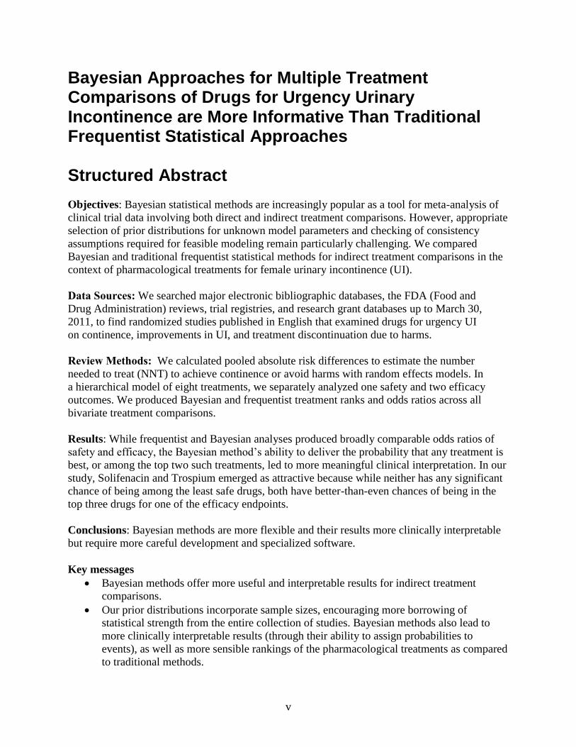
Bayesian Approaches for Multiple Treatment Comparisons of Drugs for Urgency Urinary Incontinence are More Informative Than Traditional Frequentist Statistical Approaches Structured Abstract

Objectives: Bayesian statistical methods are increasingly popular as a tool for meta-analysis of

clinical trial data involving both direct and indirect treatment comparisons. However, appropriate

selection of prior distributions for unknown model parameters and checking of consistency

assumptions required for feasible modeling remain particularly challenging. We compared

Bayesian and traditional frequentist statistical methods for indirect treatment comparisons in the

context of pharmacological treatments for female urinary incontinence (UI).

Data Sources: We searched major electronic bibliographic databases, the FDA (Food and

Drug Administration) reviews, trial registries, and research grant databases up to March 30,

2011, to find randomized studies published in English that examined drugs for urgency UI

on continence, improvements in UI, and treatment discontinuation due to harms.

Review Methods: We calculated pooled absolute risk differences to estimate the number

needed to treat (NNT) to achieve continence or avoid harms with random effects models. In

a hierarchical model of eight treatments, we separately analyzed one safety and two efficacy

outcomes. We produced Bayesian and frequentist treatment ranks and odds ratios across all

bivariate treatment comparisons.

Results: While frequentist and Bayesian analyses produced broadly comparable odds ratios of

safety and efficacy, the Bayesian method’s ability to deliver the probability that any treatment is

best, or among the top two such treatments, led to more meaningful clinical interpretation. In our

study, Solifenacin and Trospium emerged as attractive because while neither has any significant

chance of being among the least safe drugs, both have better-than-even chances of being in the

top three drugs for one of the efficacy endpoints.

Conclusions: Bayesian methods are more flexible and their results more clinically interpretable

but require more careful development and specialized software.

Key messages

Bayesian methods offer more useful and interpretable results for indirect treatment

comparisons.

Our prior distributions incorporate sample sizes, encouraging more borrowing of

statistical strength from the entire collection of studies. Bayesian methods also lead to

more clinically interpretable results (through their ability to assign probabilities to

events), as well as more sensible rankings of the pharmacological treatments as compared

to traditional methods.

vi

Further development of Bayesian methods is warranted, especially for simultaneous decision

making across multiple endpoints, assessing consistency, and incorporating data sources of

varying quality (e.g., clinical versus observational data).

vii

Contents Introduction ......................................................................................................................................1

Methods............................................................................................................................................2

Frequentist Approach .................................................................................................................2

Bayesian Approach ....................................................................................................................2

Data ............................................................................................................................................4

Results ..............................................................................................................................................6

Discussion ........................................................................................................................................9

References ......................................................................................................................................20

Abbreviations .................................................................................................................................22

Tables

Table 1. Definitions of urinary incontinence and treatment outcomes .......................................11

Table 2. Bayesian Model Comparison for Pharmacological Treatments with Outcome UI

Improvement .................................................................................................................12

Table 3. Bayesian Model Comparison for Pharmacological Treatments with Outcome

Continence .....................................................................................................................13

Table 4. Bayesian Model Comparison for Pharmacological Treatments with Outcome

Discontinuation Due to Adverse Effects .......................................................................14

Table 5. Odds Ratios and 95% Confidence Interval of Pairwise Comparisons Among

Bayes1, Bayes2 Under Homogeneous Random Effects Model, and Random

Effects Model from Frequestist Method .......................................................................18

Figures

Figure 1. Odds Ratios and Best Treatment from Three Approaches: Bayes1 (B1

Noninformative), and Bayes2 (B2 Shrinkage) Both Under the Homogeneous

Random Effects Model, and Frequentist (F) for Pharmacological Treatments with

Outcome UI Improvement .............................................................................................15




Outcome Continence .....................................................................................................16




Outcome Discontinuation Due to Adverse Effects .......................................................17

1

Introduction There is growing interest in assessing the relative effects of treatments by comparing one to

another.1-3

Because few studies are typically available to provide evidence from direct head-to-

head comparisons, we must frequently rely on indirect comparisons that use statistical

techniques to extrapolate the findings from studies of each given treatment against controls.4-8

The problem with such indirect comparisons is that the circumstances of each study and the

samples examined may vary. In addition, controls may differ among studies.

A number of techniques have been proposed to address this challenge.6-8

We applied

variations of Bayesian approaches to a data set that examines the effects of drug treatment for

urgency urinary incontinence (UI). Urgency incontinence is defined as involuntary loss of urine

associated with the sensation of a sudden, compelling urge to void that is difficult to defer.9

Continence (complete voluntary control of the bladder) has been considered a primary goal

in UI treatment10, 11

and is the most important outcome associated with quality of life in women

with UI.12

We conducted a systematic literature review that analyzed clinical efficacy and comparative

effectiveness of pharmacological treatments for urgency UI in adult women.13

We synthesized

rates of continence, improvements in UI, and discontinuation of the treatments due to harms of

drugs from 83 randomized controlled trials (RCTs) using random effects models.13

This review

utilized traditional frequentist meta-analysis techniques and concluded that drugs for urgency UI

have comparable effectiveness, and that the magnitude of the benefits from such drugs is small.

As such, treatment decisions should be made based on comparative safety of the drugs. Few

head-to-head trials were available to provide direct estimates of the comparative effectiveness of

the drugs.

Indirect comparisons, which use the relationships of treatments to controls in the absence of

direct head-to-head comparisons, can be extended to multiple comparisons over more than three

arms. By synthesizing direct and indirect comparisons, we can improve the precision of log-

relative risk estimates, and a Bayesian analysis permits explicit posterior inference regarding the

probability that each treatment is “best” for a specific outcome.

Two major issues to be considered in multiple treatment comparisons meta-analysis are

statistical heterogeneity and evidence inconsistency.14

Statistical heterogeneity represents effect

size variability between studies. Since each study is conducted under different conditions and

populations, effect sizes from each study could vary even when the true treatment effect is

equivalent in each study. Evidence inconsistency is another source of incompatibility that arises

between direct and indirect comparisons. In many multiple treatment comparisons, it is possible

to make both direct and indirect comparisons for some pairs of treatments. When discrepancies

exist between direct and indirect comparisons in terms of size and directionality, these deviations

are called evidence inconsistency.

We applied both Bayesian and frequentist statistical approaches to estimate the comparative

effectiveness and safety of selected drugs15, 16

and analyze the relative value of the more

advanced but computationally more demanding Bayesian approach.

2

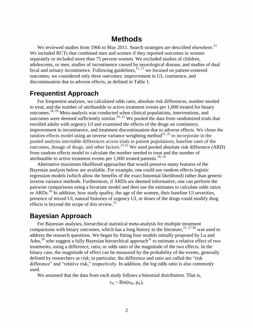
Methods We reviewed studies from 1966 to May 2011. Search strategies are described elsewhere.

13

We included RCTs that combined men and women if they reported outcomes in women

separately or included more than 75 percent women. We excluded studies of children,

adolescents, or men, studies of incontinence caused by neurological disease, and studies of dual

fecal and urinary incontinence. Following guidelines,11, 17

we focused on patient-centered

outcomes; we considered only three outcomes: improvement in UI, continence, and

discontinuation due to adverse effects, as defined in Table 1.

Frequentist Approach For frequentist analyses, we calculated odds ratio, absolute risk differences, number needed

to treat, and the number of attributable to active treatment events per 1,000 treated for binary

outcomes.18, 19

Meta-analysis was conducted when clinical populations, interventions, and

outcomes were deemed sufficiently similar.20, 21

We pooled the data from randomized trials that

enrolled adults with urgency UI and examined the effects of the drugs on continence,

improvement in incontinence, and treatment discontinuation due to adverse effects. We chose the

random effects model using an inverse variance weighting method21, 22

to incorporate in the

pooled analysis inevitable differences across trials in patient populations, baseline rates of the

outcomes, dosage of drugs, and other factors.23-25

We used pooled absolute risk difference (ARD)

from random effects model to calculate the number needed to treat and the number of

attributable to active treatment events per 1,000 treated patients.18, 19

Alternative maximum likelihood approaches that would preserve many features of the

Bayesian analysis below are available. For example, one could use random effects logistic

regression models (which allow the benefits of the exact binomial likelihood) rather than generic

inverse variance methods. Furthermore, if ARDs are deemed informative, one can perform the

pairwise comparisons using a bivariate model and then use the estimates to calculate odds ratios

or ARDs.26

In addition, how study quality, the age of the women, their baseline UI severities,

presence of mixed UI, natural histories of urgency UI, or doses of the drugs could modify drug

effects is beyond the scope of this review.13

Bayesian Approach For Bayesian analyses, hierarchical statistical meta-analysis for multiple treatment

comparisons with binary outcomes, which has a long history in the literature,21, 27-30

was used to

address the research questions. We began by fitting four models initially proposed by Lu and

Ades,29

who suggest a fully Bayesian hierarchical approach31

to estimate a relative effect of two

treatments, using a difference, ratio, or odds ratio of the magnitude of the two effects. In the

binary case, the magnitude of effect can be measured by the probability of the events, generally

defined by researchers as risk; in particular, the difference and ratio are called the “risk

difference” and “relative risk,” respectively. In addition, the log odds ratio is also commonly

used.

We assumed that the data from each study follows a binomial distribution. That is,

rik ~ Bin(nik, pik),

3

where rik is the total number of events, nik is the total number of subjects, and pik is the

probability of the outcome in the kth

treatment arm from the ith

study. Logistic regression is

commonly used to fit this type of data. The model can be written as

logit(pik) = µiB + dkB,

where B represents a baseline treatment (usually placebo), µiB is the effect of the baseline

treatment in the ith

study, and dkB is the log odds ratio between the kth

treatment and the baseline

treatment. In what follows, we drop ‘B’ from the indices, and considered it to be placebo.

Models Our first three models are fitted under the evidence consistency assumption. Model 1 is a

purely fixed effects model that doesn’t allow variability among studies. In this model, we assume

the log odds ratios, dk, are the same in each study. To model heterogeneity between studies,

random effects models may be considered. In this approach, dk is replaced with δik, which

represents a log odds ratio between treatment k and placebo in the ith

study, and we assume an

independent normal specification for the δik, i.e.,

δik ~ N(dk, σ2).

By assigning a distribution to δik, the model can capture the variability among studies, with

dk interpreted as an average relative effect of treatment k versus placebo. In this random effects

model, we assume homogeneous variance σ2 across all k treatments; we call this Model 2.

Alternatively, we can introduce heterogeneous variances σk2 across treatments. We refer to this

as Model 3. For a multi-arm trial, there are more than two log odds ratios, and one can account

for correlations among them. In this case, we assume δikvector follows a multivariate normal

distribution with common correlation of 0.5 among treatment, and we used conditional normal

distribution for each element of δik.29

Our last model allows for evidence inconsistency by adding a set of terms called w-factors

into the model. This approach captures the discrepancy between direct and indirect comparisons

between two treatments (say, 2 and 3) as

d32 = d3C – d2C + wC32,

where C indicates the common comparator treatment and wC32 is the w-factor between drugs 2

and 3 through the baseline treatment. One can only define the w-factor when the three relative

effects (d32, d3C, and d2C in the above equation) are estimable from independent studies. We

denote the homogeneous random effects model augmented by w-factors as Model 4.

Prior Distributions

Noninformative Prior In Bayesian analysis, prior information can be explicitly incorporated. We investigate two

sets of prior distribution: one fully noninformative (or “flat”) prior and another that encourages

shrinkage of the random effects toward their grand means. In the first approach, which we term

“Bayes1”, the µi and dk are assumed to have a normal prior distribution with mean 0 and

variance 10000, a specification that is very vague (though still proper) and essentially treats them

as distinct, fixed effects. For the standard deviation σ in a homogeneous random effects model, a

Uniform (0.01, 2) prior is adopted. For the heterogeneous model, a more complex prior for σk2 is

introduced; namely, we set logσk = logσ0 + υk, where σ0 ~ Uniform (0.01, 2), υk ~ N(0, ψ2), and

4

ψ is a constant chosen to reflect heterogeneity among arms. For our inconsistent model (Model

4), the w-factor has a N(0, σw2) where σw ~ Uniform (0.01, 2).

Shrinkage Prior Turning to the second prior (“Bayes2”), we incorporate the sample sizes into the prior so that

we can shrink our estimates toward each other with those from smaller, less reliable estimates

shrinking more. Under this prior, the δik are distributed N(dk, σ2/nik) instead of N(dk, σ

2), and the

µi are distributed N(mμ, τ2/ni), where ni is the sample size of the trial’s placebo arm. The

hyperparameter σ has a Uniform (0.01, 50) prior while τ has a Uniform (0.01, 50) prior; the dk

remain as N(0, 10000). We picked the upper limits of the priors for σ and τ by considering the

range of sample sizes in our data.

Model Selection Regarding methods for Bayesian model choice, the Deviance Information Criterion (DIC) is

a hierarchical modeling generalization of the familiar Akaike Information Criterion (AIC) often

used in scenario like ours.32

DIC can be calculated by summing , a measure of goodness of fit

having a posterior predictive interpretation, and pD, an effective number of parameters capturing

overall model “size,” a quantity inappropriately measured by AIC due to the presence of random

effects. Smaller values of DIC correspond to preferred models. A DIC difference of 5 or more is

generally regarded as practically meaningful.31

Decisionmaking

Probability of Being the Best Treatment The primary goal of a multiple treatment comparison is to identify the best treatment.

Suppose Pk is the posterior probability of a particular event under treatment K, perhaps modeled

with a logit function. Then if the event is a positive outcome we define the loss function as Tk =

1 – Pk, so that a treatment with the smallest loss will be the best treatment. We then define the

“Best1” probability as

Pr{K is the best treatment | Data} = Pr{rank(Tk) = 1 | Data}.

Probability of Being Among the Two Best Treatments Similarly, one can calculate the probability of being the first or second best treatment,

denoted by “Best12,” by replacing the right hand side of the above equation with Pr{rank(Tk) = 1

or 2 | Data}.

Absolute Risk Difference Versus Posterior Probability of Outcome Difference To compare with the ARD obtained in a frequentist analysis, we calculate the posterior

probability of outcome difference (PPD). As ARDs are the difference of the pooled risk between

a drug and the placebo, PPDs are also the difference of the posterior probability of outcome (Pk)

between the kth

drug and the placebo. This value can be interpreted as the excessive rate of a

particular outcome in the kth

drug compared to placebo.

All frequentist calculations were performed using STATA (Statistics/Data analysis, 10.1)

software at 95 percent confidence limits.18, 22

All of our Bayesian results were obtained from the

5

WinBUGS software,33

using 10000 Markov chain Monte Carlo (MCMC) samples after a 5000-

sample algorithm burn-in. To check MCMC convergence, we used standard diagnostics,

including trace plots and lag 1 sample autocorrelations.

Data For frequentist analyses, we used the number of events available from all randomized parallel

groups trials. When trials included more than one arm, to avoid double-counting control subjects

we randomly split the control group into subgroups of sizes proportional to the sample sizes in

the corresponding treatment groups to which these new subgroups were matched. We used

random effects models incorporating variance from all tested comparisons.34

The advantage of

this method is that it permits inclusion of all data from all RCTs. Another limitation is that

studies not having the placebo arm as the baseline treatment are excluded because only one

common comparator is allowed in the analysis for indirect comparison.35

For Bayesian analyses, there is no need to randomly split any placebo group; each study

contributes only one estimate of its placebo effect. If, however, there were two doses of the same

drug assigned in any study, only data from the higher dose were employed.

6

Results Table 2 displays the results of all eight Bayesian models (4 models each with two possible

priors) for each seven pharmacological treatments in terms of UI improvement (as defined in

Table 1). We used two measures of treatment performance: the probability of being the best

treatment (Best1), and the probability of being among the two best treatments (Best12). Table 2

reveals a decrease in the fit statistic between the fixed effects model and random effects

models; thus, introducing randomness among studies essentially forces improved model fit. The

heterogeneous random effects model yields almost the same DIC, and for the other two

outcomes, continence and discontinuation due to adverse effects (AE), the homogeneous random

effects model generally offered the best compromise between fit and complexity (i.e., lowest

DIC); neither the addition of w-factors nor heterogeneous variances paid statistically significant

dividends. As such, in Figures 1-3 below, we adopt the homogeneous random effects models.

In the lower (“Best1” and “Best12”) portion of Table 2, we see that under the Bayes1 prior,

Propiverine has 0.572 probability of being best under the fixed effects model but has a slightly

smaller probability of being best (0.510) under the homogeneous random effects model. That is,

if we introduce random effects into the model, this handles the variability across studies and

adjusts the posterior probability of being best. We can interpret the 0.510 Best1 probability by

saying that Propiverine has a roughly 50 percent chance of being the best drug, while the other

drugs together all share the remaining 50 percent chance of being best. The use of Best12 tends

to magnify differences between the best and worst drugs. For example, under the Bayes1 the

difference in Best1 probabilities between Propiverine and Tolterodine is 0.510, whereas their

difference increases to 0.721 when we consider Best12.

Figure 1 displays the Best1, Best12 probabilities, and posterior probability difference (PPD)

under the Bayes1 (B1) and Bayes2 (B2) priors with associated odds ratios and confidence limits

for each drug’s improvement relative to placebo (all calculated with the homogeneous random

effects model). The posterior probability of the outcome under placebo is 0.26, so adding this

amount to the PPD columns in Figure 1 produces the raw posterior probabilities of the outcome

for each drug. Odds ratios are computed under the Bayes1 prior. This material is comparable to

what would be produced in a traditional frequentist analyses. All of the odds ratios displayed in

Figure 1 are greater than 1 (that is, all drugs are more effective than placebo), and with the

exception of Trospium, the 95 percent credible sets of the odds ratios all exclude 1. The odds

ratio of Propiverine, Oxybutynin, and Solifenacin exceed 2, meaning that being treated with

either of these leads to more than two times greater odds of UI improvement compared to being

untreated. For this outcome, Propiverine has at least a 0.5 probability of being best across all

models, and a greater than 0.7 probability of being the first or second best. The runner-up here

appears to be Oxybutynin, which emerges with the second highest probabilities of being best or

among the top two. Tolterodine again fares worst. The drugs in Figure 1 are ranked in decreasing

order of Best12 probabilities under both priors (“Rank.B1” and “Rank.B2”) and the ranks of the

top three drugs are identical. Best drugs (Propiverine and Solifenacin) have slightly higher and

Trospium and Fesoterodine slightly lower Best12 probability under Bayes2 than Bayes1. This is

because the difference is made more obvious by shrinking when the evidence is clear.

We also provide more traditional frequentist rankings (“Rank.F”) based on the size of each

drug’s classical number needed to treat (NNT)36

as previously described in the methods section.

We calculated NNT using pooled significant absolute risk differences, and our frequentist

analyses included all data from RCTs. Frequentist analysis did not rank treatments that failed to

7

differ significantly from placebo; note the unranked treatment here (Trospium) also does not

differ significantly from placebo in the Bayesian analysis. Here the Bayesian and classical ranks

are fairly similar although they differ with the next outcome—continence, as described below.

Similarly, the frequentist ARD values are fairly close to the corresponding Bayesian PPD values,

though the former are computed simply using pooled raw risks.

Table 3 displays the results from the three models under two priors with respect to the

continence outcome, defined as absence of any involuntary leakage of urine (see Table 1). Model

4 could not be fitted because no inconsistency w-factors were identified by these data; there are

not enough studies having independent sources of direct and indirect comparisons to make these

factors estimable. There is no information on Darifenacin because none of the studies included a

Darifenacin arm for continence. There are no significant differences in DIC across the three

models, and the Best1 and Best12 probabilities are similar under Bayes1 prior. Across all six

models, Trospium is the best drug based on Best12 probability, suggesting the effect of

Trospium is dominant regardless of the presence of random effects or a shrinkage prior.

Figure 2 follows the same format as Figure 1 but with the continence outcome. Again we use

Model 2 (homogeneous random effects model) to perform the analysis; Note that the results

indicate a roughly three-way tie between Trospium, Oxybutynin, and Propiverine. All odds ratios

are significantly different from 1 (i.e., this value is excluded from 95 percent credible sets).

Trospium, Oxybutynin, and Propiverine have fitted odds ratios around 2. Overall, Trospium and

Oxybutynin appear to have a slight edge, with Tolterodine appearing to be the worst drug to cure

UI, given its smallest probabilities of being first and first or second best. The frequentist rankings

based on NNT are rather different, with Propiverine emerging as a clear winner, followed by a

three-way tie for third place.

Table 4 shows the model comparisons with respect to the safety outcome, discontinuation

due to adverse effects. Since the outcome now has a negative meaning, “Worst1” and “Worst12”

are now interpreted as being worst or being first or second worst, respectively. There is a roughly

10 unit decrease in DIC, resulting from a decrease in pD between the Bayes1 and Bayes2 priors

across all models. Also, we can see dramatic decrease in DIC between Models 1 and 2 under the

Bayes2 prior. In this specific dataset, the shrinkage encouraged by this prior implies lower model

complexity. Under both Bayes1 and 2 priors, Oxybutynin is the worst drug with the highest

Worst12 probability from all models.

Figure 3 compares the seven drugs with respect to the discontinuation outcome. Figure 3

reveals Oxybutynin has the highest probability of being least safe drug under the random effects

models, followed by Fesoterodine, with Oxybutynin and Fesoterodine presenting odds ratios

greater than 2. Tolterodine has 0 probability of being the first or second least safe drug,

suggesting it is safest among the seven treatments. All ranks agree with the first three least safe

drugs; then Bayesian ranks yield a three-way tie for last place (safest). Frequentist ranks are also

fairly similar here, with the last three drugs (Darifenacin, Solifenacin, and Tolterodine) unranked

as their discontinuation due to AE rates do not significantly differ from that of placebo.

Table 5 presents odds ratios and 95 percent confidence intervals for all pairwise comparisons

under both our Bayesian analyses (Bayes1 and Bayes2) and a frequentist analysis carried out

with the random effects model and Peto method, respectively. Although most drugs are

significantly effective compared to placebo with all outcomes, there is only one significant odds

ratio (Tolterodine versus Trospium) with continence outcome, two with the UI improvement

outcome (Oxybutynin and Propiverine versus Tolterodine), and three with the discontinuation

AE outcome (Tolterodine versus Fesoterodine and Oxybutynin and Trospium versus Oxybutynin)

8

under the Bayes1. The Bayes2 prior occasionally find significance where Bayes1 does not,

presumably due to the greater shrinkage encouraged by the former. The Bayesian analyses

generally give wider 95 percent confidence intervals than the frequentist method because the

Bayesian approach incorporates all sources of uncertainty into the model. However, note the

Bayes2 does sometimes find significance where the frequentist method does not; see e.g.

Tolterodine versus Fesoterodine and Solifenacin for continence and UI improvement, and also

Darifenacin versus Fesoterodine and Oxybutynin for discontinuation due to AE. Moreover, since

studies having no placebo arm as their baseline treatment were excluded in the frequentist

analysis, the frequentist odds ratios could be biased.

In summary, while frequentist and Bayesian analyses produced broadly comparable odds

ratios of safety and efficacy, the Bayesian method’s ability to deliver the probability that any

treatment is best, or among the top two such treatments, leads to more meaningful clinical

interpretation. For example, under the Bayes1 homogeneous random effects model, among the

pharmacological treatments, Propiverine and Oxybutynin are the most effective drugs and

Tolterodine, Darifenacin, and Fesoterodine appear to be the worst drugs for UI improvement as a

result of multiple direct and indirect comparisons. For continence, Trospium, Oxybutynin, and

Propiverine deliver the best outcomes, whereas Tolterodine is least effective. Turning to safety,

Tolterodine, Solifenacin, and Trospium are the safest drugs while Oxybutynin, Festoterodine,

and Propiverine are least safe. Thus, while Tolterodine is the safest drug, it performs worst for

UI improvement and continence. On the other hand, Propiverine works best for continence and

UI improvement, but it is one of the least safe drugs. Solifenacin and Trospium emerge as

attractive drug options because, while neither has any significant chance of being among the

least safe drugs, both have better than even chances of being in the top three drugs for one of the

efficacy endpoints (UI improvement and continence, respectively). As such, these two drugs may

be viewed (at least informally) as offering the best compromise between safety and efficacy in

this investigation.

9

Discussion Our results indicate that Bayesian methods can avoid certain biases to which traditional

frequentist methods succumb, as well as providing substantially more information useful for

clinicians and health policymakers. Theoretically, Bayesian methods score due to their more

rigorous mathematical foundation and their ability to incorporate all available sources of

information in a model-based framework, rather than simply attempt to combine p-values in

some way. From a more practical point of view, Bayesian methods offer direct probability

statements about patient-centered outcome variables, such as the probability that one drug is the

best or among the top two drugs for an indication, or the probability of experiencing a particular

endpoint given the patient takes a particular drug. The frequentist analyses relied on traditional

notions of statistical significance, and therefore did not provide an estimate of the probability of

being the best drug. The Bayesian methods remedied this shortcoming leading to practical

recommendations.

In the specific context of our UI data, both the frequentist and Bayesian meta-analyses

concluded that most of the drugs were better than placebo in achieving continence and improving

UI. Differences in efficacy among the drugs were often insignificant, but the Bayesian

probabilities of being the best or among the top two most efficacious (or safest) drugs were often

of practical significance. There were also occasional differences in drug rankings, as seen in

Figure 2, where Propiverine’s ranking drops from 1 using the frequentist approach to just 2 or 3

in the Bayesian, apparently due to high variability in this drug’s data that was improperly

acknowledged by the frequentist method. Even though Bayesian odds ratios did not show many

statistically significant differences between study drugs in the odds of continence or improving

UI, we were able to identify the drugs that were more efficacious as well as those having the

highest odds of discontinuation due to adverse effects. Combining these sets of results enables an

informed decision as to which drugs should be used, based on a joint assessment of their

probabilities of being the most effective and the safer. Of course, a sensible threshold for the

probability for being the most effective and safe drug may vary depending on the topic and the

appropriateness of the model and prior, which may of course be checked statistically.

Both our Bayesian and frequentist analyses utilized random effects, and thus avoided the

assumption of common outcome rates in the placebo groups across trials. This is important here,

since female placebo continence rates in our RCTs varied widely across Fesoterodine (48

percent), Oxybutynin (15 percent), Solifenacin (28 percent), Tolterodine (44 percent), and

Trospium (17 percent). It is well known that indirect comparisons that ignore this problem can be

biased and misleading.23

Clinicians and patients need to know rates of the benefits and harms to

make informed decisions. The number needed to treat and numbers of events attributable to

active treatment derived from frequentist analyses provide useful information for clinicians, but

their interpretation is often difficult for patients. Bayesian analysis provides a cognitively

appealing probability of the outcome that easily leads to identifying the best and the worst

treatment for each measure of the benefits and harms. A single estimate of the balance between

benefits and harms would be the most simple and actionable information for making informed

decisions in clinical settings.

Our study has several limitations. In both the Bayesian and frequentist models, we were not

able to adjust for study quality, doses of the drugs, age of the women, their baseline UI severities,

or their natural histories of urgency UI. Since we utilize every available UI study in our

likelihood, we did not attempt to specify an informative prior, but we did employ a partially

10

informative prior by incorporating sample sizes into prior (our Bayes2 prior) to encourage more

shrinkage among less reliable studies. Also, while our Bayes2 prior was partially informative, we

did not incorporate specific prior information regarding efficacy or safety for any drug due to

limited information about natural history of urgency UI. We also did not analyze all available

adverse effects from the drugs.

Broad recommendations regarding choice among Bayesian and frequentist models await

simulation studies where performance and rankings of the methods can be compared in settings

where the true state of nature (say, that the indirect evidence is inconsistent with the direct) is

known. Finally, fully Bayesian methods for formally combining both efficacy and safety data

into a single decision rule would be a significant aid in making a sensible overall decision. We

hope to address these and other methodological issues in a future publication.

11

Table 1. Definitions of urinary incontinence and treatment outcomes

Outcomes Definition

Improvement in UI Reduction frequency and severity of incontinence episodes by >50% Reduction in pad stress test by >50% Reduction in restrictions of daily activities due to incontinence Women’s perception of improvement in their bladder condition

Continence Absence of any involuntary leakage of urine Author’s reports of cure, absence of incontinent episodes in bladder diaries, negative pad stress, or no abnormalities noted on urodynamics

Discontinuation of treatment due to adverse effect

Subject refusal to continue treatment due to adverse effects or physician decision to withdraw treatment due to adverse effects

12

Table 2. Bayesian model comparison for pharmacological treatments with outcome UI improvement

Model 1

Fixed effects Bayes1

Model 1 Fixed effects

Bayes2

Model 2 Random effects (homogeneous)

Bayes1


Bayes2

Model 3 Random effects (heterogeneous)

Bayes1


Bayes2

Model 4 Random effects (inconsistency)

Bayes1


Bayes2

DIC 440.7 440.6 434.5 434.1 434.1 434.7 434.4 435.1

405.7 406.0 388.9 387.0 389.0 387.0 388.4 387.9

pD 35.0 34.6 45.6 47.1 45.1 47.7 46.0 47.2

Best1

Darifenacin 0.009 0.006 0.022 0.022 0.017 0.027 0.017 0.023

Fesoterodine 0.006 0.006 0.016 0.010 0.025 0.016 0.012 0.009

Oxybutynin 0.209 0.205 0.225 0.258 0.215 0.225 0.290 0.302

Propiverine 0.572 0.579 0.510 0.506 0.486 0.516 0.476 0.458

Solifenacin 0.146 0.180 0.183 0.190 0.200 0.195 0.161 0.190

Tolterodine 0.000 0.000 0.000 0.000 0.000 0.000 0.000 0.000

Trospium 0.058 0.025 0.045 0.015 0.058 0.020 0.045 0.019

Best12

Darifenacin 0.031 0.028 0.072 0.072 0.060 0.078 0.052 0.068

Fesoterodine 0.054 0.052 0.096 0.080 0.112 0.104 0.080 0.070

Oxybutynin 0.556 0.566 0.571 0.584 0.547 0.562 0.634 0.652

Propiverine 0.779 0.794 0.721 0.739 0.710 0.740 0.723 0.702

Solifenacin 0.430 0.486 0.424 0.479 0.439 0.464 0.396 0.455

Tolterodine 0.000 0.000 0.000 0.000 0.001 0.000 0.001 0.000

Trospium 0.151 0.074 0.116 0.047 0.131 0.052 0.114 0.055

Best1: probability of being first best drug Best12: probability of being first or second best drug Bayes1: noninformative prior Bayes2: prior with shrinkage DIC: Bayesian model choice statistic

: Bayesian model fit

pD: Bayesian effective model size

13

Table 3. Bayesian model comparison for pharmacological treatments with outcome continence

Model 1

Fixed effect Bayes1

Model 1 Fixed effect

Bayes2


Bayes1


Bayes2


Bayes1


Bayes2

DIC 284.8 284.6 286.4 289.5 286.8 286.3

259.7 259.8 258.2 258.9 258.6 259.0

pD 25.1 24.8 28.2 27.6 28.2 27.3

Best1

Darifenacin NA NA NA NA NA NA

Fesoterodine 0.017 0.047 0.045 0.045 0.052 0.062

Oxybutynin 0.329 0.292 0.296 0.299 0.338 0.293

Propiverine 0.298 0.361 0.281 0.370 0.302 0.329

Solifenacin 0.036 0.041 0.033 0.040 0.034 0.041

Tolterodine 0.000 0.000 0.000 0.000 0.000 0.000

Trospium 0.321 0.259 0.345 0.246 0.274 0.276

Best12

Darifenacin NA NA NA NA NA NA

Fesoterodine 0.083 0.165 0.152 0.157 0.167 0.201

Oxybutynin 0.560 0.496 0.548 0.511 0.564 0.475

Propiverine 0.523 0.570 0.471 0.569 0.503 0.520

Solifenacin 0.177 0.188 0.173 0.156 0.152 0.220

Tolterodine 0.000 0.000 0.002 0.000 0.002 0.000

Trospium 0.658 0.581 0.654 0.606 0.612 0.584

Best1: probability of being first best drug Best12: probability of being first or second best drug Bayes1: noninformative prior Bayes2: prior with shrinkage DIC: Bayesian model choice statistic



14

Table 4. Bayesian model comparison for pharmacological treatments with outcome discontinuation due to adverse effects

Model 1

Fixed effects Bayes1

Model 1 Fixed effects

Bayes2


Bayes1


Bayes2


Bayes1


Bayes2


Bayes1


Bayes2

DIC 601.2 593.3 598.7 585.2 596.7 585.0 600.3 585.4

547.5 547.2 531.8 525.6 529.5 525.6 531.2 524.4

pD 53.7 46.1 66.9 59.6 67.2 59.4 69.1 61.0

Worst1

Darifenacin 0.008 0.002 0.008 0.004 0.004 0.006 0.005 0.005

Fesoterodine 0.291 0.217 0.306 0.287 0.279 0.248 0.312 0.252

Oxybutynin 0.450 0.683 0.367 0.568 0.420 0.609 0.384 0.596

Propiverine 0.250 0.097 0.314 0.135 0.292 0.130 0.291 0.135

Solifenacin 0.001 0.001 0.003 0.004 0.004 0.006 0.005 0.005

Tolterodine 0.000 0.000 0.000 0.000 0.000 0.000 0.000 0.000

Trospium 0.000 0.000 0.003 0.003 0.001 0.002 0.003 0.007

Worst12

Darifenacin 0.024 0.014 0.029 0.018 0.023 0.024 0.020 0.022

Fesoterodine 0.715 0.790 0.683 0.765 0.668 0.730 0.685 0.733

Oxybutynin 0.828 0.944 0.758 0.877 0.803 0.885 0.757 0.870

Propiverine 0.416 0.220 0.484 0.273 0.456 0.287 0.481 0.278

Solifenacin 0.008 0.018 0.023 0.039 0.027 0.043 0.032 0.050

Tolterodine 0.000 0.000 0.000 0.000 0.000 0.000 0.000 0.000

Trospium 0.010 0.014 0.024 0.028 0.021 0.031 0.026 0.046

Worst1: probability of being first worst drug Worst12: probability of being first or second worst drug Bayes1: noninformative prior Bayes2: prior with shrinkage DIC: Bayesian model choice statistic



15

Figure 1. Odds ratios and best treatment from three approaches: Bayes1 (B1 noninformative), and Bayes2 (B2 shrinkage) both under the homogeneous random effects model, and frequentist (F) for pharmacological treatments with outcome UI improvement

Best1: probability of being first best drug Best12: probability of being first or second best drug NNT: number needed to treat Rank: rank of drug based on Best12 for Bayesian and NNT for frequentist PPD: posterior probability difference ARD: absolute risk difference

16

Figure 2. Odds ratios and best treatment from three approaches: Bayes1 (B1 noninformative), and Bayes2 (B2 shrinkage) both under the homogeneous random effects model, and frequentist (F) for pharmacological treatments with outcome continence

Best1: probability of being first best drug Best12: probability of being first or second best drug NNT: number needed to treat Rank: rank of drug based on Best12 for Bayesian and NNT for frequentist PPD: posterior probability difference ARD: absolute risk difference

17

Figure 3. Odds ratios and best treatment from three approaches: Bayes1 (B1 noninformative), and Bayes2 (B2 shrinkage) both under the homogeneous random effects model, and frequentist (F) for pharmacological treatments with outcome discontinuation due to adverse effects

Worst1: probability of being first worst drug Worst12: probability of being first or second worst drug NNT: number needed to treat Rank: rank of drug based on Worst12 for Bayesian and NNT for frequentist PPD: posterior probability difference ARD: absolute risk difference

18

Table 5. Odds ratios and 95% confidence interval of pairwise comparisons among Bayes1, Bayes2 under homogeneous random effects model, and random effects model from frequentist method

Active (control)

UI Improvement

Bayes1

UI Improvement

Bayes2

UI Improvement Frequentist

Continence Bayes1

Continence Bayes2

Continence Frequentist

Discontinuation Due to AE

Bayes1


Bayes2


Frequentist

Fesoterodine (Darifenacin)

1.14 (0.75 - 1.72)

1.14 (0.75 - 1.72)

0.92 (0.65 - 1.31)

1.69 (0.95 - 3.01)

1.68 (1.00 - 2.90)

1.52 (0.95 - 2.45)

Oxybutynin (Darifenacin)

1.33 (0.85 - 2.08)

1.34 (0.82 - 2.17)

1.45 (1.00 - 2.11)

1.75 (0.97 - 2.98)

1.81 (1.06 - 3.16)

1.45 (0.84 - 2.51)

Propiverine (Darifenacin)

1.45 (0.85 - 2.50)

1.45 (0.84 - 2.55)

1.43 (0.97 - 2.12)

1.56 (0.74 - 3.66)

1.37 (0.69 - 2.75)

1.85 (0.88 - 3.87)

Solifenacin (Darifenacin)

1.27 (0.76 - 2.09)

1.29 (0.78 - 2.12)

1.28 (0.91 - 1.81)

1.19 (0.68 - 2.04)

1.27 (0.77 - 2.13)

1.08 (0.71 - 1.65)

Tolterodine (Darifenacin)

0.94 (0.63 - 1.39)

0.91 (0.60 - 1.35)

0.94 (0.70 - 1.26)

0.90 (0.52 - 1.48)

0.94 (0.58 - 1.57)

0.88 (0.53 - 1.46)

Trospium (Darifenacin)

1.02 (0.55 - 1.79)

0.90 (0.46 - 1.60)

1.10 (0.71 - 1.69)

1.13 (0.62 - 1.97)

1.21 (0.71 - 2.11)

1.19 (0.74 - 1.91)

Oxybutynin (Fesoterodine)

1.16 (0.87 - 1.57)

1.17 (0.85 - 1.65)

1.58 (1.13 - 2.19)

1.13 (0.77 - 1.72)

1.10 (0.73 - 1.65)

1.16 (0.80 - 1.69)

1.03 (0.69 - 1.60)

1.07 (0.73 - 1.55)

0.95 (0.58 - 1.56)

Propiverine (Fesoterodine)

1.27 (0.82 - 2.01)

1.27 (0.84 - 1.99)

1.55 (1.09 - 2.21)

1.09 (0.73 - 1.73)

1.14 (0.76 - 1.73)

1.15 (0.78 - 1.68)

0.93 (0.45 - 2.00)

0.81 (0.44 - 1.46)

1.22 (0.60 - 2.45)

Solifenacin (Fesoterodine)

1.11 (0.75 - 1.66)

1.13 (0.79 - 1.65)

1.39 (1.03 - 1.87)

1.02 (0.77 - 1.32)

1.02 (0.80 - 1.28)

1.06 (0.83 - 1.36)

0.70 (0.45 - 1.10)

0.75 (0.53 - 1.06)

0.71 (0.50 - 1.01)

Tolterodine (Fesoterodine)

0.82 (0.67 - 1.01)

0.80 (0.67 - 0.94)

1.01 (0.79 - 1.30)

0.82 (0.67 - 1.00)

0.81 (0.69 - 0.95)

0.86 (0.65 - 1.14)

0.53 (0.38 - 0.74)

0.56 (0.43 - 0.73)

0.57 (0.37 - 0.90)

Trospium (Fesoterodine)

0.89 (0.52 - 1.45)

0.78 (0.45 - 1.27)

1.19 (0.80 - 1.78)

1.16 (0.84 - 1.56)

1.12 (0.85 - 1.47)

1.19 (0.89 - 1.58)

0.67 (0.41 - 1.08)

0.72 (0.49 - 1.04)

0.78 (0.52 - 1.18)

Propiverine (Oxybutynin)

1.08 (0.68 - 1.78)

1.09 (0.67 - 1.80)

0.99 (0.68 - 1.44)

0.98 (0.57 - 1.60)

1.03 (0.62 - 1.81)

0.99 (0.64 - 1.53)

0.91 (0.44 - 1.92)

0.76 (0.40 - 1.40)

1.27 (0.60 - 2.70)

Solifenacin (Oxybutynin)

0.95 (0.62 - 1.47)

0.97 (0.61 - 1.52)

0.88 (0.64 - 1.22)

0.90 (0.59 - 1.30)

0.92 (0.64 - 1.38)

0.91 (0.66 - 1.26)

0.69 (0.44 - 1.02)

0.70 (0.48 - 1.02)

0.74 (0.48 - 1.16)

Tolterodine (Oxybutynin)

0.70 (0.54 - 0.91)

0.68 (0.49 - 0.92)

0.64 (0.49 - 0.85)

0.73 (0.48 - 1.05)

0.74 (0.50 - 1.10)

0.74 (0.52 - 1.05)

0.52 (0.37 - 0.70)

0.52 (0.38 - 0.72)

0.60 (0.36 - 1.02)

Trospium (Oxybutynin)

0.77 (0.43 - 1.26)

0.67 (0.36 - 1.14)

0.76 (0.50 - 1.15)

1.03 (0.64 - 1.52)

1.02 (0.67 - 1.56)

1.03 (0.72 - 1.46)

0.65 (0.42 - 0.95)

0.67 (0.48 - 0.94)

0.82 (0.50 - 1.34)

Solifenacin (Propiverine)

0.87 (0.52 - 1.48)

0.89 (0.53 - 1.48)

0.90 (0.63 - 1.27)

0.93 (0.61 - 1.40)

0.90 (0.56 - 1.33)

0.92 (0.66 - 1.29)

0.76 (0.37 - 1.44)

0.93 (0.53 - 1.61)

0.58 (0.30 - 1.14)

Tolterodine (Propiverine)

0.65 (0.41 - 0.98)

0.63 (0.40 - 0.94)

0.65 (0.48 - 0.89)

0.75 (0.49 - 1.12)

0.71 (0.46 - 1.07)

0.75 (0.52 - 1.07)

0.57 (0.27 - 1.13)

0.69 (0.38 - 1.24)

0.47 (0.23 - 0.98)

Trospium (Propiverine)

0.70 (0.37 - 1.28)

0.61 (0.32 - 1.11)

0.77 (0.49 - 1.19)

1.06 (0.67 - 1.63)

0.99 (0.62 - 1.48)

1.04 (0.72 - 1.49)

0.71 (0.33 - 1.49)

0.88 (0.48 - 1.64)

0.64 (0.32 - 1.29)

Tolterodine (Solifenacin)

0.74 (0.50 - 1.08)

0.71 (0.48 - 1.00)

0.73 (0.58 - 0.93)

0.80 (0.63 - 1.05)

0.80 (0.64 - 0.99)

0.81 (0.66 - 1.00)

0.75 (0.53 - 1.09)

0.74 (0.55 - 1.02)

0.81 (0.54 - 1.21)

Table 5. Odds ratios and 95% confidence interval of pairwise comparisons among Bayes1, Bayes2 under homogeneous random effects model, and random effects model from frequentist method (continued)

19

Active (control)

UI Improvement

Bayes1

UI Improvement

Bayes2

UI Improvement Frequentist

Continence Bayes1

Continence Bayes2

Continence Frequentist


Bayes1


Bayes2


Frequentist

Trospium (Solifenacin)

0.80 (0.43 - 1.40)

0.69 (0.37 - 1.23)

0.86 (0.58 - 1.27)

1.14 (0.85 - 1.51)

1.10 (0.85 - 1.41)

1.12 (0.91 - 1.39)

0.95 (0.59 - 1.50)

0.95 (0.66 - 1.38)

1.10 (0.77 - 1.57)

Trospium (Tolterodine)

1.09 (0.64 - 1.75)

0.98 (0.57 - 1.60)

1.17 (0.82 - 1.68)

1.42 (1.04 - 1.87)

1.39 (1.05 - 1.81)

1.38 (1.07 - 1.79)

1.25 (0.82 - 1.89)

1.28 (0.90 - 1.79)

1.36 (0.86 - 2.13)

Significant odds ratios are written in bold.

20

References

1. Basu A. Economics of individualization in

comparative effectiveness research and a basis

for a patient-centered health care. 2011.

2. Committee on Comparative Effectiveness

Research Prioritization IoM. Initial National

Priorities for Comparative Effectiveness

Research. June 30 2009.

http://www.nap.edu/catalog/12648.html.

3. Institution B. Implementing comparative

effectiveness research: Priorities, methods, and

impact. The Hamilton Project. 2009 June:1-88.

4. Coory M, Jordan S. Frequency of treatment-

effect modification affecting indirect

comparisons: a systematic review.

Pharmcoeconomics. 2010;28(9):723-32.

5. Wells G, Sultan S, Chen L, et al. Indirect

evidence: Indirect treatment comparisons in

meta-analysis. Ottawa: 2009.

6. Glenny AM, Altman DG, Song F, et al. Indirect

comparisons of competing interventions. Health

Technol Assess. 2005 Jul;9(26):1-134, iii-iv.

PMID 16014203.

7. Song F, Loke YK, Walsh T, et al.

Methodological problems in the use of indirect

comparisons for evaluating healthcare

interventions: survey of published systematic

reviews. BMJ. 2009;338:b1147. PMID

19346285.

8. Donegan S, Williamson P, Gamble C, et al.

Indirect comparisons: a review of reporting and

methodological quality. PLoS One.

2010;5(11):e11054. PMID 21085712.

9. Haylen BT, de Ridder D, Freeman RM, et al.

An International Urogynecological Association

(IUGA)/International Continence Society (ICS)

joint report on the terminology for female

pelvic floor dysfunction. Neurourol Urodyn.

2010;29(1):4-20. PMID 19941278.

10. Abrams P. Incontinence: 4th International

Consultation on Incontinence, Paris, July 5-8,

2008: Health Publications Ltd: 2009.

Committee 12. Adult Conservative

Management.

11. U.S. Department of Health and Human Services,

Food and Drug Administration, Center for

Devices and Radiological Health, et al. Draft

Guidance for Industry and FDA Staff - Clinical

Investigations of Devices Indicated for the

Treatment of Urinary Incontinence. Rockville,

MD 20852: Food and Drug Administration,

5630 Fishers Lane, Room 1061; 2008.

http://www.fda.gov/MedicalDevices/DeviceReg

ulationandGuidance/GuidanceDocuments/ucm0

70852.htm. Accessed on August, 2009 2009.

12. Coyne KS, Sexton CC, Kopp ZS, et al. The

impact of overactive bladder on mental health,

work productivity and health-related quality of

life in the UK and Sweden: results from

EpiLUTS. BJU Int. 2011 Mar 3PMID

21371240.

13. Shamliyan T, Wyman J, Kane RL. Nonsurgical

Treatments for Urinary Incontinence in Adult

Women: Diagnosis and Comparative

Effectiveness. AHRQ Publication No. 11-

EHC074. Rockville, MD. Agency for

Healthcare Research and Quality.

2001;36:Prepared by the University of

Minnesota Evidence-based Practice Center

under Contract No. HHSA 290-2007-10064-I.

14. Lumley T. Network meta-analysis for indirect

treatment comparisons. Stat Med. 2002 Aug

30;21(16):2313-24. PMID 12210616.

15. Berry SM, Ishak KJ, Luce BR, et al. Bayesian

meta-analyses for comparative effectiveness

and informing coverage decisions. Med Care.

2010 Jun;48(6 Suppl):S137-44. PMID

20473185.

16. O'Regan C, Ghement I, Eyawo O, et al.

Incorporating multiple interventions in meta-

analysis: an evaluation of the mixed treatment

comparison with the adjusted indirect

comparison. Trials. 2009;10:86. PMID

19772573.

17. Abrams P. Incontinence: 4th International

Consultation on Incontinence, Paris, July 5-8,

2008. 4th ed. [Paris]: Health Publications Ltd.;

2009.

http://www.nap.edu/catalog/12648.html

http://www.fda.gov/MedicalDevices/DeviceRegulationandGuidance/GuidanceDocuments/ucm070852.htm



21

18. Egger M, Smith GD, Altman DG. Systematic

Reviews in Health Care. London: NetLibrary,

Inc. BMJ Books; 2001.

19. Ebrahim S. The use of numbers needed to treat

derived from systematic reviews and meta-

analysis. Caveats and pitfalls. Eval Health Prof.

2001 Jun;24(2):152-64. PMID 11523384.

20. Whitehead A. Meta-analysis of controlled

clinical trials. Chichester, New York: John

Wiley & Sons; 2002.

21. DerSimonian R, Laird N. Meta-analysis in

clinical trials. Control Clin Trials. 1986

Sep;7(3):177-88. PMID 3802833.

22. Wallace BC, Schmid CH, Lau J, et al. Meta-

Analyst: software for meta-analysis of binary,

continuous and diagnostic data. BMC Med Res

Methodol. 2009;9:80. PMID 19961608.

23. Fu R, Gartlehner G, Grant M, et al. Conducting

Quantitative Synthesis When Comparing

Medical Interventions: AHRQ and the Effective

Health Care Program. Methods Guide for

Comparative Effectiveness Reviews. Rockville,

MD.: Agency for Healthcare Research and

Quality, . 2010.

24. Gartlehner G, Fleg A. Comparative

effectiveness reviews and the impact of funding

bias. J Clin Epidemiol. 2010 Jun;63(6):589-90.

PMID 20434022.

25. Fu R, Gartlehner G, Grant M, et al. Conducting

quantitative synthesis when comparing medical

interventions: AHRQ and the effective health

care program. J Clin Epidemiol. 2011 Apr

6PMID 21477993.

26. van-Houwelingen HC, Arends LR, Stijnen T.

Tutorial in biostatistics advanced methods in

meta-analysis: Multivariate approach and meta-

regression. Statistics in Medicine. 2002;21:589-

624.

27. Smith TC, Speigelhalter DJ, Thomas SL.

Bayesian approaches to random-effects meta-

analysis: a comparative study. Statistics in

Medicine. 1995;14:2685-99.

28. Nixon RM, Bansback N, Brennan A. Using

mixed treatment comparisons and meta-

regression to perform indirect comparisons to

estimate the efficacy of biologic treatments in

rheumatoid arthritis. Statistics in Medicine.

2007;26:1237-54.

29. Lu G, Ades A. Assessing evidence

inconsistency in Mixed Treatment Comparisons.

Journal of the American Statistical Association.

2006;101:447-59.

30. Lu G, Ades AE. Combination of direct and

indirect evidence in mixed treatment

comparisons. Stat Med. 2004 Oct

30;23(20):3105-24. PMID 15449338.

31. Carlin B, Louis T. Bayesian Methods for Data

Analysis. Boca Raton, FL: Chapman and

Hall/CRC Press; 2009, page 71.

32. Spiegelhalter D, Best N, Carlin B, et al.

Bayesian Measures of Model Complexity and

Fit (with Discussion). J Roy Statist Soc, Ser B.

2002;64:583-639.

33. Lunn D, Thomas A, Best N, et al. WinBUGS- a

Bayesian modelling framework: concepts,

structure, and extensibility. Statistics and

Computing. 2000;10:325-37.

34. Higgins J, Green S, Cochrane Collaboration.

Cochrane handbook for systematic reviews of

interventions. Chichester, West Sussex ;

Hoboken NJ: John Wiley & Sons; 2008.

35. Gartlehner G, Moore CG. Direct versus indirect

comparisons: a summary of the evidence. Int J

Technol Assess Health Care. 2008

Spring;24(2):170-7. PMID 18400120.

36. Altman DG. Confidence intervals for the

number needed to treat. Bmj. 1998 Nov

7;317(7168):1309-12. PMID 9804726.

22

Abbreviations AE Adverse effect

AIC Akaike information criterion

ARD Absolute risk difference

DIC Deviance information criterion

MCMC Markov chain Monte Carlo

NNT Number needed to treat

PPD Probability of outcome difference

RCT Randomized controlled trial

UI Urinary incontinence