bayesian approaches to associative learning: from …kruschke/articles/kruschke2008.pdfbayesian...

Copyright 2008 Psychonomic Society, Inc. 210

Bayesian formalizations of learning are a revolution-ary advance over traditional approaches. Bayesian mod-els assume that the learner maintains multiple candidate hypotheses with differing degrees of belief, unlike tra-ditional models that assume the learner has a punctate state of mind. Bayesian models can account for some as-sociative learning phenomena that are very challenging for traditional approaches. Perhaps more important, but even less prominent in the associative learning literature, is the fact that Bayesian models provide a foundation for models of active learning. Because Bayesian models rep-resent degrees of belief across multiple hypotheses, the active learner can assess which possible probing of the environment is most likely to achieve beliefs that reduce uncertainty or make some hypotheses highly probable. Traditional models, by contrast, typically treat the learner as a passive recipient of information, and such models offer no predictions for how a real learner would actively probe its environment.

This article is divided into two main parts. The first is a selective review of Bayesian models of associative learn-ing. Two different Bayesian models are described in detail and compared with the traditional Rescorla–Wagner (1972) model. The behavior of the models is illustrated by appli-cations to some well-known phenomena, such as backward blocking. The review also indicates how the specific mod-els are situated in the larger space of all possible Bayesian models, which offers a remarkably liberating cornucopia of representational options for models of learning.

The second part of the article focuses on active learning. Two different goals for active learning are reviewed, and the

predictions of the two Bayesian models are presented. This article is the first application of active-learning formalisms to models of associative learning. The derivations and sim-ulations demonstrate that different combinations of knowl-edge representations and active-learning goals generate dif-ferent predictions, some of which are already informed by results in the literature. The broad framework that combines Bayesian models of passive learning with various goals for active learning is a gold mine for new research.

TradiTional and Bayesian Theories

In traditional cognitive models, the learner’s knowledge at any given moment is represented as a specific state. For example, the learner may have an associative weight of 0.413 between “tone” and “shock,” or the learner may know that the concept “cat” has a value of 0.289 on the scale of ferocity. When new information is delivered by the world, the values may change. For example, if another instance of shock preceded by a tone occurs, the asso-ciative weight might then increase to 0.582. On the other hand, if a cat snuggles up and purrs, that concept’s ferocity value might decrease to 0.116. The punctate values com-prise the totality of the learner’s knowledge.

Bayesian approaches assume a radically different men-tal ontology, in which the learner entertains an entire spec-trum of hypothetical values for every descriptor. For ex-ample, the association between “shock” and “tone” might be anything on an infinite continuum, and the learner’s knowledge consists of a distribution of believabilities over that continuum. The learner may believe most strongly in

Bayesian approaches to associative learning: From passive to active learning

John K. KruschKeIndiana University, Bloomington, Indiana

Traditional associationist models represent an organism’s knowledge state by a single strength of association on each associative link. Bayesian models instead represent knowledge by a distribution of graded degrees of belief over a range of candidate hypotheses. Many traditional associationist models assume that the learner is passive, adjusting strengths of association only in reaction to stimuli delivered by the environment. Bayesian models, on the other hand, can describe how the learner should actively probe the environment to learn opti-mally. The first part of this article reviews two Bayesian accounts of backward blocking, a phenomenon that is challenging for many traditional theories. The broad Bayesian framework, in which these models reside, is also selectively reviewed. The second part focuses on two formalizations of optimal active learning: maximizing either the expected information gain or the probability gain. New analyses of optimal active learning by a Kal-man filter and by a noisy-logic gate show that these two Bayesian models make different predictions for some environments. The Kalman filter predictions are disconfirmed in at least one case.

Learning & Behavior2008, 36 (3), 210-226doi: 10.3758/LB.36.3.210

J. K. Kruschke, [email protected]

Active BAyesiAn AssociAtive LeArning 211

ditional approach is represented by the Rescorla–Wagner model. That model was selected both because it is well-known and because it has a direct Bayesian generalization, known as the Kalman filter. A second Bayesian model is also presented because, as we will see, it makes differ-ent predictions for active learning. This second Bayesian model is the noisy-logic gate.

All of the models will be applied to a basic experi-mental procedure for assessing learning. In discrete tri-als, cues are presented, and the learner is to predict the outcome. Typically, the learner’s prediction is prompted and recorded on each trial before the actual outcome is re-vealed. For example, the learner might have to learn which foods cause or prevent nausea in a particular patient. In each trial, a meal is presented consisting of a small num-ber of foods (the cues) ingested by the patient, and the outcome is whether or not the patient suffered nausea after the meal. The learner is informed that some foods may be antiemetic—that is, they prevent nausea that might other-wise be induced by other foods.

The ith cue is denoted by ci, with ci 5 1 if the cue is present and ci 5 0 if it is absent. When several cues are available, the column vector containing the cue values is denoted c.

The outcome is denoted t (for teacher), with t 5 1 if the outcome is present and t 5 0 if it is absent. Differ-ent models, described below, make different predictions regarding the outcome, whose anticipated value is de-noted a. Through learning, the anticipated value a should get closer to the correct outcome t.

An organism’s knowledge is what generates an an-ticipated outcome after cues are perceived. The learner’s knowledge can be formalized by a theorist in many differ-ent ways; the complexity of the formalization depends on the modeler’s imagination and the complexity of the learn-ing phenomena that are being addressed. In traditional as-sociative models, the learner’s knowledge is formalized simply as an associative weight between each cue and the outcome, and the weighted cues are integrated in some simple way. The weight from the ith cue is denoted wi, which can have a positive or a negative value. When there are several cues, the column vector containing the weight values from the cues is denoted w.

In traditional associative learning models, the learner’s knowledge is assumed to consist of a single weight value on each cue. For example, the learner might currently be-lieve that the first cue should have a weight of w1 5 0.9 and the second cue a weight of w2 5 0.3. Learning con-sists of changing those weight values after observing a new occurrence of cues and outcome. For example, if the learner observes Cue 2 with an outcome, then the adjusted weight values might be w1 5 0.9 (unchanged) and w2 5 0.4 (larger than before).

In Bayesian associative learning models, the learner’s knowledge is assumed to entertain simultaneously all possible combinations of weight values, with a degree of believability for each combination. At any moment in time, the learner believes most strongly in some particular weight combination, but also believes somewhat in others, and even less strongly in yet others. As mentioned before,

a value of 0.413 but also have some belief in values larger or smaller. Entertaining an infinite space of hypothetical values does not imply the need for an information proces-sor of infinite capacity, for infinite belief distributions can be represented with small sets of values. For example, a normal distribution, which extends over an infinite space, is fully represented by its mean and variance. Also, an arbi-trary infinite distribution can be represented by a finite set of sample values, just as a sample histogram approximates the underlying distribution that generated the sample.

The distribution of believabilities can be joint over mul-tiple variables, and therefore correlations among variables can be captured. For example, the learner may believe that higher values of association between “tone” and “shock” are correlated with higher values of cat ferocity.

The distribution of beliefs expresses the learner’s uncer-tainty: The more spread out the beliefs, the greater the un-certainty. Traditional models, with punctate values, have no natural way of representing the learner’s uncertainty, whereas Bayesian models represent it inherently.

Learning in a Bayesian model is shifting of beliefs. When there is another occurrence of a tone with a shock, higher values of association are more believable. The dis-tribution of believable values also narrows in that case, because the additional experience makes the learner more certain about the relation between tone and shock.

Bayesian reasoning relies on trade-offs among the be-lievabilities of the available hypotheses. We intuitively use these trade-offs in everyday reasoning. In the everyday “logic of exoneration,” if one suspect confesses, an unaffili-ated suspect is exonerated. In general, increasing the believ-ability of some hypotheses necessarily decreases the believ-ability of others; that is, the others are exonerated. Later in this article, we will encounter the phenomenon of backward blocking, which can be explained in a Bayesian framework by the logic of exoneration. A complementary form of ev-eryday reasoning is Holmesian deduction: “How often have I said to you that when you have eliminated the impossible, whatever remains, however improbable, must be the truth?” So said Sherlock Holmes in Arthur Conan Doyle’s novel The Sign of Four (1890, ch. 6). In other words, decreasing the believability of some hypotheses necessarily increases the believability of the remaining hypotheses. Later on, we will encounter the phenomenon of reduced overshadowing, which can be explained in a Bayesian framework by the logic of Holmesian deduction.

There are at least two advantages of Bayesian over tra-ditional models. First, because Bayesian models can keep track of multiple combinations of hypothetical values and their believabilities, they can account for some learning be-haviors that are challenging for traditional models. Second, because Bayesian models inherently represent the degree of uncertainty, they can be used to guide active learning, which (in one formulation) attempts to probe the environ-ment for information that will rapidly reduce uncertainty.

examples: one Traditional and Two Bayesian Models

The vague informal ideas discussed above are clarified by concrete examples presented in this section. The tra-

212 KruschKe

squared error, (t 2 a)2, yields the following formula for adjusting the weights:

Dw 5 l(t 2 a) c

5 l(t 2 wTc) c, (3)

where Dw denotes the changes in the weights and l . 0 is a learning rate parameter that governs the overall speed of learning in the model. The weights are typically all as-sumed to begin at 0 and then to change according to Equa-tion 3 on each trial.

The crucial point to understand about the Rescorla–Wagner model is that it represents the learner’s knowl-edge as a single, punctate combination of associative weights, w. At any given moment in time, the learner’s knowledge is completely specified by a single weight value on each cue. When the information from the next trial is presented, those weight values change, but the up-dated knowledge is still a single weight value on each cue. There is no representation of alternative weight combina-tions that might also account for the cue–outcome expe-riences. Nor is there any representation of the learner’s uncertainty about the weight values.

The Kalman filter. The Kalman filter was originally developed in the context of least-squares estimation for dynamic systems (Kalman, 1960), and a Bayesian formu-lation and tutorial was presented by Meinhold and Sing-purwalla (1983). The Kalman filter was introduced to associative learning theorists by Sutton (1992). More re-cently, the filter has been used by Dayan and colleagues to model various phenomena in associative learning (Dayan, Kakade, & Montague, 2000; Kakade & Dayan, 2002).

In the Kalman filter applied to associative learning, there are two crucial enhancements to the Rescorla–Wagner model that make it Bayesian. First, the anticipated outcome is not just the specific weighted sum of cue activations, as in Equation 2. Instead, it is expressed as a degree of belief over all possible outcome values. The degree of belief in outcome value a is expressed as a normal probability distri-bution centered on the weighted sum of cue activations:

p(a | c, w, n) 5 N(a | wTc, n), (4)

where N(a | m, n) denotes a normal density on a with mean m and variance n. Thus, the Kalman filter says that the most likely outcome is the weighted sum of the cues, but outcomes a little larger or smaller are also somewhat be-lievable. The value of the outcome variance, n, is a free pa-rameter in the model; it not only expresses the uncertainty of prediction, but also affects the rate of learning, as will be shown below.

The second crucial enhancement to the Rescorla– Wagner model that makes the Kalman filter Bayesian involves knowledge representation. The learner’s knowl-edge in the Kalman filter is not only a single weight value on each cue. Instead, the learner entertains all possible weight combinations across the cues, with each possible combination having a degree of belief. In the Kalman fil-ter, the distribution of beliefs is assumed to be a multivari-ate normal distribution, centered on some mean weight m. The covariance matrix of the multivariate normal distribu-

an infinite belief distribution can be represented by a fi-nite set of values. The distribution of degrees of believ-ability is formally described as a probability distribution. This formalization implies that all believabilities are non-negative and that, across the space of all possible weight combinations, the believabilities sum to 1. In a Bayesian model, the belief distribution is denoted p(w).

The other key difference between Bayesian and tradi-tional models is that Bayesian models generate probabi-listic rather than deterministic anticipations. Instead of predicting that the outcome will have a specific value a, Bayesian models predict a probability for each possible an-ticipated value. The prediction is that some value a is most probable, but that other values, a bit higher or lower, are also possible with somewhat lesser probability. The prob-ability of the possible anticipated values, given the current cues and current knowledge, is denoted p(a | c, w).

Learning in a Bayesian model consists of changing the belief distribution after observing a new occurrence of cues and outcome. The normatively correct way to change beliefs is provided by Bayes’s rule:

p t p t( | , ) ( | , )

posterior

w c c w

=likelihood

p

d p t p

( )

( | , ) ( )

w

w c w w

prior

∫. (1)

This rule says that the learned believability of a particu-lar combination of weights after observing some specific cues and outcomes, denoted p(w | t, c), is proportional to the believability of that weight combination before the observation, denoted p(w), multiplied by the probability that the observation would occur for that weight value, denoted p(t | c, w). The believability of the weights after the observation is called the posterior distribution, and the believability of the weights before the observation is called the prior distribution. The probability of the obser-vation, for a particular weight combination, is called the likelihood function of the weights.

The denominator of Equation 1 contains an integral that evaluates to a constant, p(t | c). This value is sometimes called the evidence for the model. It indicates the degree to which the observed outcome t is anticipated, when aver-aged across all possible values of the weights, scaled pro-portionally to their believabilities. The integral is rarely easy to determine with formulas alone, and therefore so-phisticated numerical approximations must be used. The last two decades have produced tractable computational methods for these approximations, and hence there is great interest in Bayesian approaches. This integral will appear again later in the article, in the context of active learning, but for now it can be ignored.

The rescorla–Wagner model. In the Rescorla– Wagner model, the predicted or anticipated outcome a is the weighted sum of the cue activations:

a 5 Si wici

5 wTc, (2)

where wT is the vector transpose of the column vector w. Learning consists of decreasing the error between the cor-rect and the anticipated outcome. Gradient descent on the


The Rescorla–Wagner learning rate l (Equation 3) has been replaced by the Kalman filter term in square brackets (Equation 6) involving the outcome uncertainty n and the belief uncertainty C. In particular, if only cue ci is present and all others are absent, the effective learning rate on that cue is [n 1 cTCc]21 5 Vi/[n 1 Vi], where Vi is the variance of the belief on the ith associative weight. In other words, when the uncertainty Vi is larger, learning is faster. This is a general property of Bayesian learning: When belief about a parameter, such as an associative weight, is highly uncertain, observational data have a rapid influence on changing that belief. On the other hand, when belief about a value is already highly certain, new data do not budge the belief very much.

In the Rescorla–Wagner learning rule (Equation 3), the rightmost term is the cue activation, c. This implies that when a cue is absent—that is, when ci 5 0—the weight on the cue does not change. In the Kalman filter formula for the change of mean, the rightmost term is the cue vec-tor times the covariance matrix—that is, Cc. This implies that when a cue is absent, the mean weight on the cue might nevertheless change, if other cues are present that are correlated with the absent cue. This characteristic will be important for the Kalman filter’s behavior when it is applied to the procedure known as backward blocking, to be described later.

The updating equation for the covariance of the beliefs across weights, Equation 7, is similar to that for the mean of the beliefs. A curious and important difference, though, is that the covariance of the beliefs does not depend on the actual outcome t. The covariance of the beliefs in the weights depends only on the particular cue combinations that have appeared! This independence from the actual outcome is a characteristic of the Kalman filter model but is not true of Bayesian models generally, as we will see below.

In summary, these are the main points to understand about the Kalman filter model. At its core is the linear as-sociator of the Rescorla–Wagner model, but the Kalman filter makes the anticipated outcome probabilistic and en-tertains all possible weight combinations with different degrees of belief. The belief distribution across weights is assumed to begin as multivariate normal, and a pleasing mathematical result is that Bayesian updating of the belief distribution maintains the multivariate normal shape of that distribution. Because the distribution remains mul-tivariate normal, the beliefs of the learner at any given moment can be summarized by the mean vector and cova-riance matrix of the multivariate normal.

The noisy-logic gate. Whereas the Kalman filter as-sumes that the output can be any value, the noisy-logic gate (see, e.g., Danks, Griffiths, & Tenenbaum, 2003; Lu, Yuille, Liljeholm, Cheng, & Holyoak, 2006; Yuille & Lu, in press) assumes that the output is 1 or 0. This is natural in many associative learning scenarios, when the outcome to be predicted does not vary in its magnitude across trials. The cues in this paradigm can, in principle, have values in the interval [0, 1], but typically they also are assumed to be discretely valued, with ci [ {0, 1}.

tion is denoted C. The degree of belief in a weight combi-nation w is expressed as the multivariate normal density:

p(w) 5 N(w | m, C )

5 [(2π)n | det(C ) | ]21/2 exp[20.5(w 2 m)T

C21(w 2 m)], (5)

where n is the number of cues and det(C ) is the deter-minant of the covariance matrix. The covariance matrix captures the current uncertainty of the learner’s beliefs; its ith diagonal element is the variance of the belief re-garding weight wi. When that variance is large, there is large uncertainty regarding the value of wi. The off-diagonal elements of the covariance matrix describe the learner’s knowledge of trade-offs between weight values. We will see concrete examples of this in the applications described below.

The Kalman filter also allows for incorporating un-learned linear dynamics into the weight changes. These dynamic changes are imposed by the theorist “from the outside” as an additional influence on the associative weights, unrelated to learning from cues and outcomes. In the applications of Dayan and colleagues (Dayan et al., 2000; Kakade & Dayan, 2002), this additional dynamic is assumed to be a random diffusion process, such that the passage of time increases uncertainty without chang-ing the mean belief. The degree of noise added with each trial is a free parameter. In the simulations that I describe below, I have set the unlearned dynamic component to 0. Without any unlearned dynamic component, the simula-tions reveal the pure learning aspects of the model. When nonzero dynamic noise is introduced, the qualitative re-sults remain the same in many situations.

Learning in the Kalman filter means shifting the de-gree of belief over all of the possible weight combinations, to take into account the observed cues and outcome. The mathematically correct way to do this is with Bayes’s rule, in Equation 1. It turns out—and this is the beauty of the Kalman filter—that when Bayes’s rule is applied to the likelihood formula in Equation 4 and the prior formula in Equation 5, the resulting expression for the updated beliefs, known as the posterior distribution, is again a mul-tivariate normal distribution over the possible weights. In other words, if the beliefs begin as a multivariate normal distribution, then, after observing some cues and an out-come, the new beliefs are still distributed in the form of a multivariate normal, but with some new mean and covari-ance. The updating equations for the mean and covariance of the beliefs have the following form:

Dm 5 [n 1 cTCc]21 (t 2 mTc)Cc (6)

DC 5 2[n 1 cTCc]21 CccTC. (7)

Notice that the updating equation for the mean (Equa-tion 6) is much like the updating equation for weights in the Rescorla–Wagner model (Equation 3). In Equation 6, the term in parentheses, (t 2 mTc), is analogous to the term (t 2 wTc) in Equation 3. Thus, both the Kalman filter and the Rescorla–Wagner model incorporate the prediction error as a factor in learning.

214 KruschKe

influences of the cues interact according to a probabilis-tic, or “noisy,” logical combination, as in Equation 8. The weights on the cues can take on values between 21 and 11. The initial knowledge state is a diffuse prior belief distribution over the space of all possible weight combi-nations, and learning proceeds according to Bayes’s rule. Unfortunately, no simple formula exists for updating the belief distribution, and therefore a numerical approxima-tion must be used.

application to Backward BlockingThe three models defined above are here applied to the

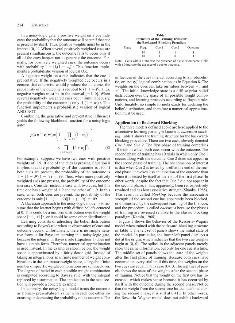
associative learning paradigm known as backward block-ing. Table 1 shows the training structure for the backward-blocking procedure. There are two cues, cleverly denoted Cue 1 and Cue 2. The first phase of training comprises 10 trials in which both cues occur with the outcome. The second phase of training has 10 trials in which only Cue 1 occurs along with the outcome. Cue 2 does not appear in the second phase of training. The phenomenon of interest is that when Cue 2 is tested by itself at the end of the sec-ond phase, it evokes less anticipation of the outcome than when it is tested by itself at the end of the first phase. In other words, despite the fact that Cue 2 did not appear in the second phase, it has, apparently, been retrospectively revalued and has lost associative strength (Shanks, 1985). This result is called blocking because the associative strength of the second cue has apparently been blocked, or diminished, by the subsequent learning of the first cue, and the procedure is called backward because the phases of training are reversed relative to the classic blocking paradigm (Kamin, 1968).

Figure 1 shows the behavior of the Rescorla–Wagner model when trained with the backward-blocking structure in Table 1. The left set of panels shows the initial state of the model. In particular, the lower left panel displays a dot at the origin, which indicates that the two cue weights begin at (0, 0). The spikes in the adjacent panels merely show the same information, but only for one cue at a time. The middle set of panels shows the state of the weights after the first phase of training. Because both cues have occurred on every trial until this time, the weights on the two cues are equal, in this case 0.413. The right set of pan-els shows the state of the weights after the second phase of training. Notice that the weight on the first cue has in-creased, which makes sense because it has occurred by itself with the outcome during the second phase. Notice that the weight from the second cue has not declined dur-ing the second phase; it is still at 0.413. In other words, the Rescorla–Wagner model does not exhibit backward

In a noisy-logic gate, a positive weight on a cue indi-cates the probability that the outcome will occur if that cue is present by itself. Thus, positive weights must be in the interval [0, 1]. When several positively weighted cues are present simultaneously, the outcome fails to occur only if all of the cues happen not to generate the outcome. For-mally, for positively weighted cues, the outcome occurs with probability 1 2 pi(1 2 wi)

ci. This function imple-ments a probabilistic version of logical OR.

A negative weight on a cue indicates that the cue is preventative. If the negatively weighted cue occurs in a context that otherwise would produce the outcome, the probability of the outcome is reduced to (1 1 wi)

ci. Thus, negative weights must be in the interval [21, 0]. When several negatively weighted cues occur simultaneously, the probability of the outcome is only p i(1 1 wi)

ci. This function implements a probabilistic version of logical AND-NOT.

Combining the generative and preventative influences yields the following likelihood function for a noisy-logic gate:

p a w

w

i

c

i w

j

i

i

( |= = − −( )

× +(≥

∏1 1 1

1

0

c w, )s.t.

))<

∏c

j w

j

j

.s.t. 0

(8)

For example, suppose we have two cues with positive weights of 1.9. If one of the cues is present, Equation 8 implies that the probability of the outcome is .90. If both cues are present, the probability of the outcome is 1 2 (1 2 .9)(1 2 .9) 5 .99. Thus, when more positively weighted cues are present, the probability of the outcome increases. Consider instead a case with two cues, but this time one has a weight of 1.9 and the other of 2.9. In this case, when both cues are present, the probability of the outcome is only [1 2 (1 2 .9)][1 1 (2.9)] 5 .09.

A Bayesian approach to the noisy-logic model is to as-sume that the learner begins with diffuse beliefs centered at 0. This could be a uniform distribution over the weight space [21, 11]N, or it could be some other distribution.

Learning consists of adjusting the belief distribution according to Bayes’s rule when an observation of cues and outcome occurs. Unfortunately, there is no simple itera-tive formula for Bayesian learning in a noisy-logic gate, because the integral in Bayes’s rule (Equation 1) does not have a simple form. Therefore, numerical approximation is used instead. In the examples shown below, the weight space is approximated by a fairly dense grid. Instead of taking an integral over an infinite number of weight com-binations in the continuous weight space, a large but finite number of specific weight combinations are summed over. The degree of belief in each possible weight combination is computed according to Bayes’s rule, with the integral replaced by a summation. The application in the next sec-tion will provide a concrete example.

In summary, the noisy-logic model treats the outcome as a binary present/absent value, with each cue either in-creasing or decreasing the probability of the outcome. The

Table 1 structure of the Training Trials for the Backward-Blocking Paradigm

Phase Freq. Cue 1 Cue 2 Outcome

I 10 1 1 1II 10 1 0 1

Note—Cells with a 1 indicate the presence of a cue or outcome. Cells with a 0 indicate the absence of a cue or outcome.


Kalman filter keeps track of all of those believable weight combinations, which have a negative covariance.

The right set of panels shows the beliefs after the sec-ond phase of training. The mean of the first weight has increased (to 0.763). Importantly, the mean of the weight from Cue 2 has decreased, from 0.417 to 0.169. In other words, the Kalman filter shows backward blocking, unlike the Rescorla–Wagner model.

The specific mathematical reason that the Kalman fil-ter decreases the mean weight of Cue 2, even when that cue is absent, is the negative correlation between Cue 2 and Cue 1. Recall from Equation 6 that the change of mean weight is proportional to Cc, not just to c as in the Rescorla–Wagner model. Therefore, the change of the mean for w2 is proportional to the covariance of Cue 2 and Cue 1, which is negative. This negative factor is a direct consequence of Bayesian updating of beliefs and is analogous to the heuristically motivated formalizations of negative activation for absent cues suggested by previous theorists (see Markman, 1989; Tassoni, 1995; Van Hamme & Wasserman, 1994).

The intuitive reason that the Kalman filter can change its mean belief about Cue 2, even when Cue 2 does not appear, is that the believabilities of the weight combina-

blocking. This failing can be deduced from the learn-ing rule itself: Equation 3 reveals that a weight does not change when the corresponding cue value is 0.

Figure 2 shows the results of training the Kalman filter on the backward-blocking procedure of Table 1. All pos-sible weight combinations have some nonzero degree of believability. The left set of panels shows the prior beliefs of the model, which make the neutral weight combination (0, 0) the most believable, and more extreme weight com-binations less believable, with probability dropping off according to a bivariate normal distribution.

The middle set of panels shows the beliefs after the first phase of training. The belief distribution is still bivariate normal, but with a different set of means and covariance matrix than at the start. In particular, the mean belief on each weight is the same, in this case 0.417. Importantly, the contour graph reveals that the beliefs regarding the weights have a negative covariance. This negative covariance re-veals which weight combinations are consistent with the observations seen to this time. The only observations seen so far have had both cues present with the outcome. Cer-tainly one weight combination consistent with those ob-servations would be (0.5, 0.5), but other weight combina-tions, such as (0, 1) and (1, 0), would also be consistent. The

Training: BackwardBlocking

Beginning of Trial 1

Mean: 0 0



Mean: 0.413 0.413



Mean: 0.745 0.413

p(w

)0

.4.8

p(w

)C

ue

2 W

t.0

.4.8

Cue 1 Wt�1.0 0.0 1.0

Cue 1 Wt�1.0 0.0 1.0

1.0

0.0

�1.

0

Cue 2 Wt�1.0 0.0 1.0

p(w

)C

ue

2 W

t0

.4.8

Cue 1 Wt�1.0 0.0 1.0

Cue 1 Wt�1.0 0.0 1.0

1.0

0.0

�1.

0

Cue 2 Wt�1.0 0.0 1.0

p(w

)C

ue

2 W

t0

.4.8

Cue 1 Wt�1.0 0.0 1.0

Cue 1 Wt�1.0 0.0 1.0

1.0

0.0

�1.

0

Cue 2 Wt�1.0 0.0 1.0

p(w

)0

.4.8

p(w

)0

.4.8

Figure 1. The rescorla–Wagner model after training with the backward-blocking structure in Table 1. The left panels show the weights prior to training. The middle panels show the weights after Training Phase i, and the right panels show the weights after Training Phase ii. For this simulation, the learning rate λ in equation 3 was arbitrarily set to 0.08.

�2 �1 0 1 2

0

.1

.2

.3

.4

Cue 1 Wt

pd

(w)

�2 �1 0 1 2

0

.

1

.

2

.3

.4

Cue 2 Wt

pd

(w)

Cue 1 Wt

Cu

e 2

Wt

�2 �1 0 1 2

�2

�1

01

2

Train: BackwardBlockingBeginning of Trial 1

Mean: 0 0Covariance matrix:

1 00 1

Current Uncertainty: 2.838Probe: 1 0 �� EU: 2.726Probe: 0 1 �� EU: 2.726

�2 �1 0 1 2

0

.2

.4

Cue 1 Wt

pd

(w)

�2 �1 0 1 2

0

.2

.4

Cue 2 Wt

pd

(w)

Cue 1 Wt

Cu

e 2

Wt

�2 �1 0 1 2

�2

�1

01

2


Mean: 0.417 0.417Covariance matrix:

.583 �.417�.417 .583


−2 −1 0 1 2

0

.

2

.

4

.

6

.

8

Cue 1 Wt

pd

(w)

�2 �1 0 1 2

0

.

2

.

4

.6

.8

Cue 2 Wt

pd

(w)

Cue 1 Wt

Cu

e 2

Wt

�2 �1 0 1 2

�2

�1

01

2


Mean: 0.763 0.169Covariance matrix:

.237 �.169�.169 .407


Figure 2. The Kalman filter after training with the backward-blocking structure in Table 1. The left panels show the distribution of beliefs prior to training. The middle panels show the distribution of beliefs after Training Phase i, and the right panels show the distribution after Training Phase ii. For this simulation, the output variance n in equation 4 was arbitrarily set to 4, and the initial covariance matrix C was set to the identity matrix.

216 KruschKe

In summary, the Rescorla–Wagner model does not ex-hibit backward blocking, but both Bayesian models do. The Kalman filter can be thought of as a direct Bayesifica-tion of the Rescorla–Wagner model, in that both models generate an anticipated outcome that is a weighted sum of the cues. The noisy-logic model uses a different func-tion to combine weighted cue information. Both Bayesian models qualitatively exhibit backward blocking because they implement the logic of exoneration: If Cue 1 is re-sponsible for the outcome, then Cue 2 probably is not. Later in this article, the two Bayesian models will be shown to make different predictions for active learning. Before taking up this topic, however, I will explore the space of possible Bayesian models a bit more.

other Bayesian Models of associative learningAs illustrated above by the application of both the Kal-

man filter and noisy-logic models to backward blocking, there is no single Bayesian model for a particular situation. Different Bayesian models can make different predictions. In this section, I describe another class of Bayesian mod-els for associative learning, called generative models. These address the fact that learners learn about the cues, as well as cue–outcome correspondences, during associa-tive learning. I then describe an overarching framework in which the learner’s theory of the domain determines the space of hypotheses over which Bayesian learning is executed. This framework helps answer the question of, for example, whether a Kalman filter or a noisy-logic model is more appropriate for a particular learning situ-ation. Finally, I describe an even broader framework that considers learning at different levels of analysis, such that components within a learning system might conduct lo-cally Bayesian learning, whereas the system as a whole might not be globally Bayesian. Systems of locally Bayes-ian models can address learning phenomena that are chal-lenging for globally Bayesian models.

Generative versus discriminative models. The Kal-man filter and the noisy-logic gate both associate cues with outcomes, not cues with other cues or outcomes with

tions trade off: When the model increases believability in weight combinations such as (1, _) during the second phase, it has to decrease believability in weight combina-tions such as (_ , 1). Even more intuitively, the model is reasoning this way: If Cue 1 is responsible for the out-come, then Cue 2 probably is not. This is the everyday logic of exoneration.

Figure 3 shows the results of training the noisy-logic gate with the backward-blocking structure in Table 1. The left panels show the distribution of beliefs prior to training. To make the initial state comparable to that of the Kalman filter, the prior belief was set to a bivariate normal distribution with a covariance matrix equal to the identity matrix. The distribution was truncated at 61 (be-cause the weights in the noisy-logic model are restricted to that range) and then renormalized so that the total be-lief probability across all possible weight combinations was 1.0.

The middle set of panels shows the state of the beliefs after the first phase of training. The beliefs regarding the two weights are symmetric, because both cues have appeared in every trial. Notice that weight values near 11.0 are believed in more strongly than smaller positive weights, and negative weight values have very weak belief probability. The contour plot reveals that the joint belief distribution is not bivariate normal. Instead, it is bimodal, with one peak near (0, 1) and the other near (1, 0). In words, the joint distribution suggests that either Cue 1 or Cue 2 indicates the outcome, but maybe not both.

The right set of panels shows the state of the beliefs after the second phase of training. The model now loads most of its belief regarding Cue 1 on high weight values, but it has shifted beliefs regarding weights on Cue 2 toward lower values. In other words, the noisy-logic model shows backward blocking. The intuitive reason for this back-ward blocking is, as in the Kalman filter, the logic of ex-oneration: In the second phase, weights of the form (1, _) are consistent with the Phase II observations. As beliefs in those weight combinations increase, beliefs in other weight combinations, such as (_ , 1), must decrease.

Cue 1 Wt

p(w

)

Cue 2 Wt

p(w

)

Cue 1 Wt

Cu

e 2

Wt



Current Uncertainty: 0.993

Probe: 1 0 �� EU: 0.952

Probe: 0 1 �� EU: 0.952

Cue 1 Wt

p(w

)Cue 2 Wt

p(w

)

Cue 1 WtC

ue

2 W

t




Probe: 1 0 �� EU: 0.708

Probe: 0 1 �� EU: 0.708

Cue 1 Wt

p(w

)

Cue 2 Wt

p(w

)

Cue 1 Wt

Cu

e 2

Wt




Probe: 1 0 �� EU: 0.568

Probe: 0 1 �� EU: 0.5430

0.0 0.5 1.0�1.0

.4.8

0

0.0 0.5 1.0�1.0

.4.8

0

0.0 0.5 1.0�1.0

.4.8

0

0.0 0.5 1.0�1.0

.4.8

0

0.0 0.5 1.0�1.0

.4.8

0.0

0.0 0.5 1.0�1.0

0.5

1.0

�1.

0

0

0.0 0.5 1.0�1.0

.4.8

0.0

0.0 0.5 1.0�1.0

0.5

1.0

�1.

0

0.0

0.0 0.5 1.0�1.0

0.5

1.0

�1.

0

Figure 3. The noisy-logic gate after training with the backward-blocking structure in Table 1. The left panels show the distribution of beliefs prior to training. The middle panels show the distribution of beliefs after Training Phase i, and the right panels show the distribution after Training Phase ii. For this simulation, each weight interval [21, 11] was arbitrarily divided into 33 equally spaced points, yielding 332 5 1,089 weight combinations. The prior probability was a (truncated) bivariate normal distribution with a standard deviation of 1, renormalized so that the total probability was 1.0 across the 1,089 weight combinations.


less show a transition to conditioned inhibition through continued training.

The point of this subsection has not been to claim that Bayesian models are uniquely capable of showing a transi-tion from second-order conditioning to conditioned inhi-bition. On the contrary, there may, in principle, be many non-Bayesian models that produce such behavior. Rather, the point has been to illustrate two additional aspects of Bayesian models: First, the Bayesian approach can be applied to generative as well as discriminative models, and second, the prior beliefs in a Bayesian model can be crucial to its behavior. The next subsection again empha-sizes the important role of prior beliefs, but over a much broader hierarchy of model representations.

Theories to generate hypothesis spaces. In the previ-ous sections, I described three different Bayesian models of associative learning—namely, the Kalman filter, the noisy-logic gate, and a generative model. All three use weighted connections to cues and outcomes, but with different ar-chitectures and functional forms. Where do these archi-tectures and functional forms come from? And how does a researcher, or a learner, decide which model best accounts for data? An answer to these questions comes naturally from a hierarchical Bayesian framework, in which higher-level theories generate specific model spaces and Bayesian learn-ing updates beliefs within the model spaces and across theo-ries simultaneously. The general approach is described by Tenenbaum, Griffiths, and Kemp (2006) and Tenenbaum, Griffiths, and Niyogi (2007). Specific examples of its ap-plication have been presented by Kemp, Perfors, and Tenen-baum (2004), Griffiths and Tenenbaum (2007), and Good-man, Tenenbaum, Feldman, and Griffiths (2008).

In the general approach, the first step is to define the learner’s theory of the domain being learned about. One aspect of the theory is the learner’s ontology of the do-main. For example, are there different classes of entities, such as cues, outcomes, and latent causes? What are the allowed predicates—that is, the properties—of these enti-ties? For example, can an outcome have only the values “present/absent,” or can an outcome have a continuum of possible values? Another aspect of the theory is the set of allowed relations among entities, which defines the implications of some predicates for other predicates. For example, one allowed implication may be as follows: If a cue is present, it may be true that an outcome is pres-ent. A final aspect of the theory specifies the functional form of the relationships. For example, the activations of cues could be combined via weighted summation to pro-duce an outcome activation, as in the Kalman filter, or via weighted products, as in the noisy-logic gate.

The fully specified theory then generates the space of all possible hypotheses. Every allowed combination of entities and their predicates, relations, and function forms is placed into a hypothesis space. In this way, instead of the hypothesis space being a heuristic assumption by the theorist, its assumptions are made explicit and attributed to the learner’s theory regarding the domain. Even more importantly, the theory establishes the prior distribution of beliefs over the hypothesis space. One especially use-ful way to establish the prior is to have the space of hy-

cues. These models are sometimes called discriminative because they discriminate among cues to predict an out-come. This aspect of the Kalman and noisy-logic models is explicit in the form of their likelihood functions, which specify the probability of an outcome value given a cue combination and the model’s weight value: p(a | c, w)—for example, Equations 4 and 8.

Other models can be invented, however, that learn the cues too. These models are called generative because they generate the cue values, rather than merely discriminate among them. Formally, the likelihood function of a gener-ative model specifies the probability of a combination of outcome value with cue values, given the model’s weights: p(a, c | w).

A recent application of a generative Bayesian model to associative learning comes from Courville and col-laborators (Courville, Daw, Gordon, & Touretzky, 2004; Courville, Daw, & Touretzky, 2006). In their specific formulation, every cue and outcome is assumed to be a binary-valued feature. These features are linked to under-lying latent causes. These causes are not explicit in the observable features; they are hypothetical constructs in the mind of the learner. The task for the learner is to figure out which are the most plausible combinations of latent causes to account for the observed cue and outcome com-binations. Each hypothetical latent-cause combination has particular weighted associations with particular cues and outcomes, and each hypothetical cause has a degree of believability. Since this is a Bayesian framework, there is a vast space of candidate latent causes, and learning consists of shifting degrees of belief across the candidate latent causes, such that the ones most consistent with the observations become more strongly believed.

The system begins with prior beliefs that emphasize “simple” structures—that is, those with few latent causes, few features connected to the causes, and small magnitude weights. As data are observed during training, the prior bias on simplicity can be overwhelmed by complexity in the data. The prior bias on simplicity, with a transition to more complex beliefs through training, has been fruit-fully used to account for learners’ transition from second-order conditioning to conditioned inhibition (Courville et al., 2004) . In conditioned inhibition, the learner experi-ences cases of Cue 1 producing the outcome, along with many other cases of the combination of Cues 1 and 2 not producing the outcome. When subsequently tested with Cue 2 alone, the learner does not anticipate an outcome. Indeed, if Cue 2 is combined with another cue that has been previously learned to indicate the outcome, then the outcome is still not anticipated. In other words, Cue 2 has been learned to be an inhibitor of the outcome. Both the Kalman filter and the noisy-logic gate can show such conditioned inhibition. Curiously, however, if the train-ing contains only a few, rather than many, cases of Cue 1 with Cue 2 not producing the outcome, Cue 2 is often learned to be a positive indicator of the outcome rather than an inhibitor (Yin, Barnet, & Miller, 1994). It is as if the learner has inferred a second-order link to the outcome via Cue 1. Neither the Kalman filter nor the noisy-logic gate can exhibit second-order conditioning at all, much

218 KruschKe

There has been debate as to whether or not individual people are Bayesian in their learning, because some sim-ple learning behaviors are prima facie not Bayesian (e.g., see the references cited in Kruschke, 2006b). One way to address this problem is to rethink the level of analysis. Whereas individual learning might not be Bayesian, inte-rior components of the learner might be. The main mes-sage of this subsection is that the level of analysis should not be taken for granted, and locally Bayesian learning need not behave the same as globally Bayesian learning.

FroM Passive To acTive learninG

The learning models discussed up to this point have all assumed that the learner is a passive observer. In most real learning situations, however, the learner has the op-portunity to explore or manipulate the world in order to extract information that is believed will be useful. The learner actively selects the next query rather than waiting for whatever the world happens to display next.

Traditional models of associative learning have few, if any, ways to select a useful query for the next learning trial. Current knowledge is represented only by a specific set of weight values, with no indication of which are more or less certain than the others. Therefore, the model pro-vides no guidance as to which weight values need to be bolstered by additional data.

Bayesian models, on the other hand, inherently repre-sent uncertainty, with each candidate weight combination carrying a belief probability. Depending on the exact goal of the learner, the distribution of beliefs can be used to select a query that is likely to yield much more useful in-formation than would a random event passively observed. The present article is the first application of active learn-ing to Bayesian models of associative learning.

“active learning” in Traditional TheoriesThe phrase active learning has been used in a different

way from the one in this section by some proponents of traditional theories. In particular, Spence (1950, p. 169) wrote: “Quite contrary to its opponents’ claims, then, the S–R theory does not assume that the animal passively re-ceives all the physically present stimuli. . . . The early stages of learning situations . . . involve, as an important part of them, the acquisition of . . . receptor exposure adjustments that provide the relevant cue. Such learning is itself an ac-tive, trial-and-error process . . .” (emphasis added).

Despite the fact that Spence (1950) called the selection of relevant cues an active process, it is not active in the sense I mean here. Selective attention, in traditional theo-ries, merely filters or amplifies stimuli that are controlled entirely by the experimenter and are passively received by the learner. A variety of models created in recent years have addressed the learning of selective attention (see, e.g., Kruschke, 2001). These models learn what cues to attend to, given stimuli that are passively received. Indeed, Spiker (1977, p. 99) argued that this sort of learning should not be called “active,” but should instead be called “reactive.”

For learning to be active in the sense meant here, the learner must have the potential to manipulate the next

potheses specified by a generative grammar on entities, predicates, and functional forms. Each production rule in the grammar specifies how particular hypotheses are generated from a root. Each production rule has a prob-ability of application, and the probability of a hypothesis is the product of the probabilities of the productions used to generate it. There is insufficient space here to review the details of this approach; the reader is encouraged to consult Goodman et al. (2008) and Kemp (2008) for de-tailed examples.

The Bayesian approach encourages hierarchical mod-els, wherein it is natural to suppose that the learner has multiple candidate theories that might apply to any given learning domain. The learner learns which hypotheses within a theory are most believable and, simultaneously, which theories are most believable. For example, a learner could entertain one theory that generates Kalman hypoth-eses and a second theory that generates noisy-logic hy-potheses. The Bayesian learner will shift beliefs regarding the theories in the same way she or he shifts beliefs regard-ing hypotheses within theories. The Bayesian approach offers a natural formalism wherein the representational richness of complex learning can be accommodated.

locally Bayesian learning. All the models discussed above have a shared assumption, that the entity that learns is an individual: an individual person, an individual rat, an individual pigeon. Other levels of analysis are possible, however. Within an individual person, single neurons can be modeled as learning entities (see, e.g., Deneve, 2008). Likewise, across individual persons, committees or hier-archies of people can be modeled as learning entities (e.g., Akgün, Byrne, Lynn, & Keskin, 2007). Any of these learn-ing entities could be modeled, in principle, as a Bayesian learner. If a component of a system learns in a Bayesian manner, what is the resulting behavior of the molar system that combines the components? The answer must depend on how the components are combined.

One approach to locally Bayesian learning is to assume a hierarchy of learners, who get information from only their immediate inferiors or superiors in the hierarchy. The environmental cues and outcomes impinge on learn-ers only at the bottom and top of the hierarchy. Learners embedded in the middle of the hierarchy have no direct contact with the cues and outcomes, but instead get infor-mation that has been transformed by their inferiors and superiors. Nevertheless, each learner adjusts its beliefs in a Bayesian manner, on the basis of the information it is given. This sort of structure may occur in many domains, from brains to corporations.

Locally Bayesian learning has been applied to phenom-ena from associative learning (Kruschke, 2006a, 2006b). In that application, one level of the hierarchy learned which cues to attend to, and the next level learned associations from attended cues to outcomes. This locally Bayesian learning model was able to exhibit phenomena that other Bayesian models cannot. In particular, when the hypothesis space was changed to include all possible combinations of attentional allocation and associations, the resulting glob-ally Bayesian model could not account for some human be-havior that the locally Bayesian model mimicked.


distribution comes from information theory and is called the entropy of the distribution. I will use the term uncer-tainty instead. The uncertainty of a probability distribution p(w) is

U p pi ii

w w= − ( ) ( )∑ log ( ) ,w (9)

where the sum is over all possible values that w can have. When w is a continuous variable, the corresponding for-mula becomes an integral instead of a finite sum (and, technically, the result is referred to as the differential en-tropy). The uncertainty is maximized when p(w) is uni-form, and minimized when p(w) is a spike.

What we would like to do is select a cue c so that when the outcome a is observed, the uncertainty Uw | a,c of the posterior distribution p(w | a, c) is as small as possible. Un-fortunately, we do not know in advance what the outcome a will be when c occurs, but we can guess on the basis of our current beliefs. The probability of outcome value a, given cue c and particular associative weights w, is specified by the likelihood formula for the model, p(a | c, w). The degree to which we expect outcome value a for cue c, averaged across all possible associative weights, is just the sum of the probabilities of a for any particular w value, weighted by the probability that we believe in each particular w. Mathematically, p(a | c) 5 e dw p(a | c, w) p(w). (This is the denominator of Bayes’s rule—Equation 1—when a 5 t.) Once we have determined the probability of each outcome value a given cue c, we can determine the expected poste-rior uncertainty if cue c were to occur:

EU da p a Uw ( ) ( | ) w| ,c c c= ∫ a . (10)

An active learner’s goal is to determine the cue c that minimizes expected uncertainty in Equation 10, and then to probe with that cue. The resulting observed outcome should yield, on average, a relatively large reduction in uncertainty regarding the associative weights.

It turns out that Equation 10 is particularly simple to compute for the Kalman filter. The uncertainty of a multi-variate normal distribution depends on its covariance ma-trix, not on its mean. Importantly, for the Kalman filter, the covariance matrix depends only on the cues, not the outcomes, as can be gleaned from Equation 7. Therefore, the integral in Equation 10 collapses into merely the un-certainty of a multivariate normal, which is well-known: U 5 0.5 log[(2eπ)n | det(C ) | ], where C is the covariance matrix after updating with the candidate c.

For the noisy-logic model, Equation 10 is also easy to compute, because there are only two possible outcome val-ues. Therefore, the integral reduces to a sum over the two possible values of the outcome: EUw(c) 5 p(a 5 1 | c) Uw | a51,c 1 p(a 5 0 | c) Uw | a50,c. The values for p(a | c) and Uw | a,c are approximated by summing over the grid on the associative weights.1

expected Uncertainty after Backward BlockingFigures 2 and 3 display the expected uncertainties if

the model were to probe next with either Cue 1 by itself—denoted “Probe: 1 0”—or Cue 2 by itself—“Probe: 0 1.” An active learner whose goal is to reduce uncertainty as

stimulus, to intervene in the world. Active learning in-volves choosing which cues or cue combinations would be most informative to learn about. These cues might or might not be the ones that have been attended to; indeed, the cues that one has learned to ignore are often also those about which one is most uncertain, and therefore the cues that one would like to learn about the most. The cues that an active learner would choose to learn about are not necessarily the ones that would be delivered in an experimenter-chosen reinforcement schedule. Examples are presented in the subsequent sections.

Minimizing expected UncertaintyWhen the learner has the opportunity to seek new infor-

mation for learning, what type would be the best to seek? What is the precise goal to be achieved by active learning? Although there are many possible goals, I will focus here on maximizing the expected information gain. Nelson (2005) summarized several different goals that an active learner might plausibly have, and he reviewed a number of articles in the psychological literature that utilized ex-pected information gain as the goal for the learner. Ex-pected information gain (or closely related goals) has also been used extensively by researchers in machine learning and artificial intelligence (e.g., Denzler & Brown, 2002; Laporte & Arbel, 2006; Paletta, Prantl, & Pinz, 2000; Tong & Koller, 2001a, 2001b).

Intuitively, the goal is to seek the information that will probably reduce uncertainty by the greatest amount. As an example, suppose that you experienced the backward-blocking procedure, as in Table 1. During the training, you experienced some trials of Cues 1 and 2 occurring together with the outcome, and you experienced other tri-als of Cue 1 alone occurring with the outcome. At the end of training, which cue would you be most uncertain about? If allowed to actively create a trial in which a cue occurred by itself, which cue would you probe? Intuitively, it seems that the status of Cue 1 would be fairly certain, because it had occurred by itself in several trials with the outcome. You would be less certain about Cue 2, because it had oc-curred only with Cue 1, so whether or not it independently predicted the outcome would not be clear. Therefore, a probe of Cue 2 by itself, to see whether or not the out-come occurred, would reduce uncertainty a lot. Presenting Cue 1 by itself, on the other hand, would merely confirm the already known. Thus, probing with Cue 2 would maxi-mize the expected information gain. This intuition is now given a precise formal definition.

First we must define the uncertainty of the current knowledge state. In Bayesian associative models, knowl-edge is a probability distribution over possible associative weight combinations. When that probability distribution is tightly peaked over a specific weight combination, the model is very certain that those weight values are the ones that best account for the observed data. When the prob-ability distribution is flat and spread out over vast regions of the weight space, the model is then very uncertain about what weights best account for the observations. Thus, un-certainty corresponds to the flatness or spread of the belief distribution. A natural measure of spread of a probability

220 KruschKe

learners were asked, “If you had the possibility to see one additional event, would you like to see what would hap-pen if the patient only ate [Food Cue 2] or would you like to see what would happen if the patient only ate [Food Cue 4]?” (Vandorpe & De Houwer, 2006, p. 1134). The results confirmed the prediction: Every learner preferred to test Food Cue 2—that is, the blocked cue—instead of the reduced overshadowed one. Learners also made rat-ings of how useful it would be to test with Cue 2 or Cue 4. Ratings of usefulness were far higher for the blocked than for the reduced overshadowed cue.

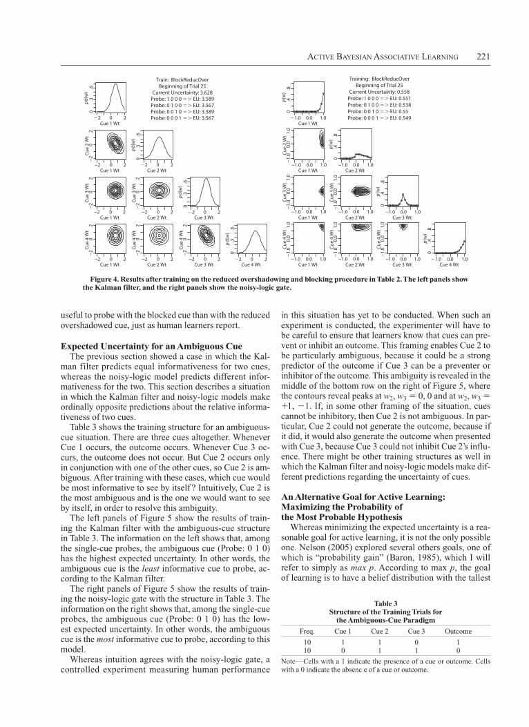
When the Kalman filter is trained with the items in Table 2, it shows equal uncertainty for the blocked and reduced overshadowed cues. The precise results are dis-played on the left side of Figure 4. The expected uncer-tainty after probing with the blocked cue (Probe: 0 1 0 0) is 3.567, which is exactly the same as what would be ex-pected after probing with the reduced overshadowed cue (Probe: 0 0 0 1). This equivalence is not merely a coinci-dence, but is mathematically implied by the nature of the Kalman filter. As was mentioned above, the uncertainty of the Kalman filter is determined by its covariance matrix, and the covariance matrix depends only on the cue struc-ture, not the outcomes. The cue structures for blocking and reduced overshadowing are identical: Both structures involve a single cue occurring on some trials and that cue occurring with another on other trials. Because the cue structure is the same, the covariance matrix is the same. The equivalence of the covariances can be seen on the left side of Figure 4: The panel that displays the Cue 2 weight against the Cue 1 weight shows the same oval pattern as the panel that displays the Cue 4 against the Cue 3 weight, with merely the mean differing between panels. Thus, the Kalman filter does not show the difference in uncertainty that people show between blocked and reduced overshad-owed cues.

When the noisy-logic gate is trained with the items in Table 2, it shows differential uncertainty for the blocked and reduced overshadowed cues, as people do. The precise results are displayed on the right side of Figure 4. The panels on the diagonal show that this model has fairly strong beliefs about the reduced overshadowed cue (Cue 4 weight) but relatively diffuse beliefs about the blocked cue (Cue 2 weight). The expected uncertainty after probing with the blocked cue (Probe: 0 1 0 0) is 0.538, which is less than the expected uncertainty of 0.549 after probing with the reduced overshadowed cue (Probe: 0 0 0 1). In other words, the noisy-logic gate predicts that it would be more

quickly as possible should choose the probe that yields the lowest expected uncertainty. The rightmost panel of Figure 2 shows that the Kalman filter yields a lower uncer-tainty if Cue 2 is probed (1.463 vs. 1.444 for the two cues). The rightmost panel of Figure 3 shows that the noisy-logic model also yields a lower uncertainty if Cue 2 is probed (0.568 vs. 0.543). The magnitudes of the expected uncer-tainties should not be compared across models, because they are on different scales. In this application, therefore, the two models agree with each other and with the intu-ition explained at the beginning of this section: We are fairly confident that Cue 1 predicts the outcome, because we have seen many cases of exactly that, but we are uncer-tain about Cue 2, because we have never seen it by itself. Therefore, a probe involving only Cue 2 would be more informative than a probe involving only Cue 1.

expected Uncertainty after Blocking and reduced overshadowing

Another well-established phenomenon in associative learning is called mutual overshadowing of cues. Two cues that always occur together, along with an outcome, seem to acquire less associative strength than either cue would if it occurred alone with the outcome the same number of times. This pattern of training occurs in the first phase of backward blocking (see Table 1), and the mutual overshadowing of associative strengths is exhib-ited by the Rescorla–Wagner model, the Kalman filter, and the noisy-logic gate (see the middle panels of Figures 1, 2, and 3).

In the so-called reduced overshadowing procedure, the training of two cues with an outcome is preceded by a phase in which one of the cues occurs alone and with no outcome. In this way, the learner is given the opportunity to notice that one of the cues does not indicate the out-come. Subsequently, the two cues occur together, and the outcome does occur. By the logic of Holmesian deduction, described in the introduction, the second cue should gar-ner greater association with the outcome, because the first cue is not responsible. In other words, the overshadowing of the second cue by the first should be reduced.

Reduced overshadowing and (forward) blocking have been studied by Vandorpe and De Houwer (2006), who predicted that learners should have very different uncer-tainties about a blocked cue versus a reduced overshad-owed cue. Vandorpe and De Houwer reasoned that a blocked cue can be ambiguous, because of the intuitions discussed earlier, but a reduced overshadowed cue is much less ambiguous, because it clearly does predict the out-come. Vandorpe and De Houwer trained people with the structure shown in Table 2. Learners were instructed that they were to figure out what foods produced an allergic reaction in a particular fictitious patient. On each trial of training, a learner was shown a “meal” that the patient consumed and whether or not an allergic reaction fol-lowed. Each meal consisted of one or more foods. Each cue in Table 2 corresponds to a particular food (mush-rooms, kiwi, fish, or potatoes) that could be present or ab-sent in the meal. After training on the 24 meals in Table 2,

Table 2 structure of the Training Trials

for reduced overshadowing and Blocking

Phase Freq. Cue 1 Cue 2 Cue 3 Cue 4 Outcome

I 6 1 0 0 0 16 0 0 1 0 0

II 6 1 1 0 0 16 0 0 1 1 1

Note—Cells with a 1 indicate the presence of a cue or outcome. Cells with a 0 indicate the absence of a cue or outcome.


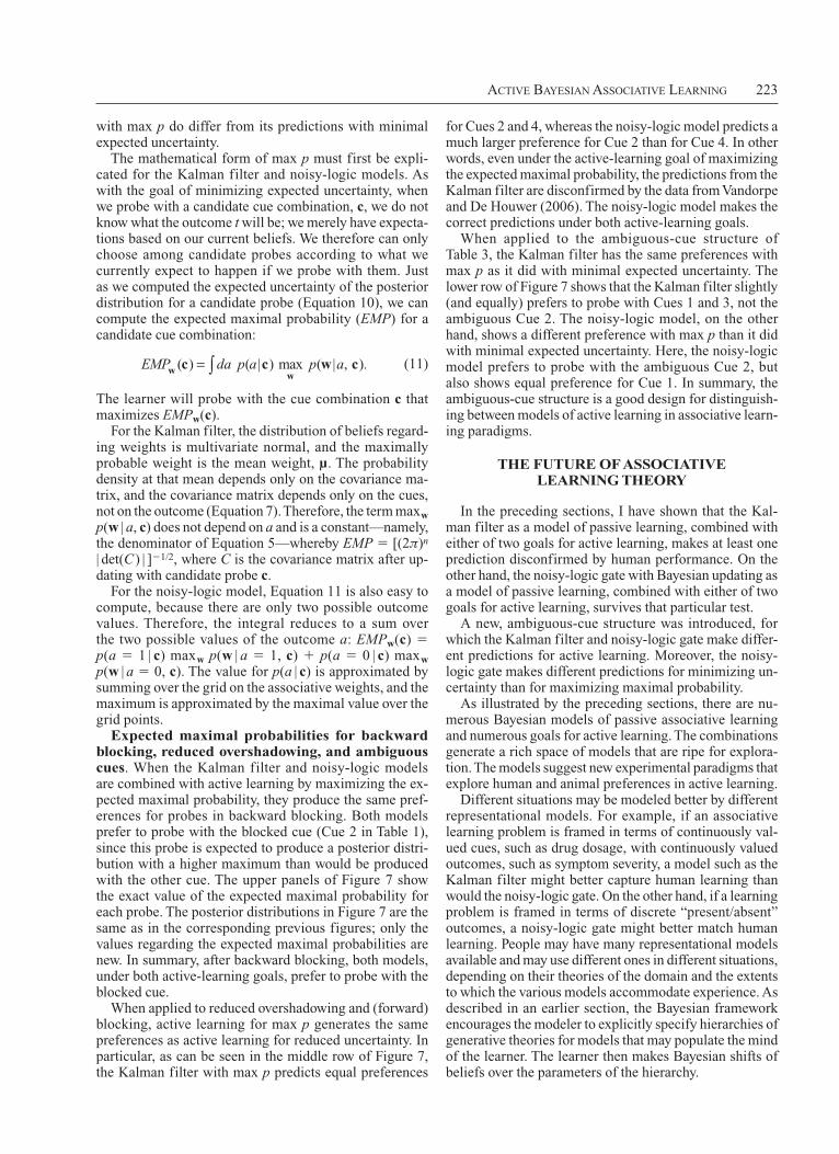
in this situation has yet to be conducted. When such an experiment is conducted, the experimenter will have to be careful to ensure that learners know that cues can pre-vent or inhibit an outcome. This framing enables Cue 2 to be particularly ambiguous, because it could be a strong predictor of the outcome if Cue 3 can be a preventer or inhibitor of the outcome. This ambiguity is revealed in the middle of the bottom row on the right of Figure 5, where the contours reveal peaks at w2, w3 5 0, 0 and at w2, w3 5 11, 21. If, in some other framing of the situation, cues cannot be inhibitory, then Cue 2 is not ambiguous. In par-ticular, Cue 2 could not generate the outcome, because if it did, it would also generate the outcome when presented with Cue 3, because Cue 3 could not inhibit Cue 2’s influ-ence. There might be other training structures as well in which the Kalman filter and noisy-logic models make dif-ferent predictions regarding the uncertainty of cues.

an alternative Goal for active learning: Maximizing the Probability of the Most Probable hypothesis

Whereas minimizing the expected uncertainty is a rea-sonable goal for active learning, it is not the only possible one. Nelson (2005) explored several others goals, one of which is “probability gain” (Baron, 1985), which I will refer to simply as max p. According to max p, the goal of learning is to have a belief distribution with the tallest

useful to probe with the blocked cue than with the reduced overshadowed cue, just as human learners report.

expected Uncertainty for an ambiguous cueThe previous section showed a case in which the Kal-

man filter predicts equal informativeness for two cues, whereas the noisy-logic model predicts different infor-mativeness for the two. This section describes a situation in which the Kalman filter and noisy-logic models make ordinally opposite predictions about the relative informa-tiveness of two cues.

Table 3 shows the training structure for an ambiguous-cue situation. There are three cues altogether. Whenever Cue 1 occurs, the outcome occurs. Whenever Cue 3 oc-curs, the outcome does not occur. But Cue 2 occurs only in conjunction with one of the other cues, so Cue 2 is am-biguous. After training with these cases, which cue would be most informative to see by itself ? Intuitively, Cue 2 is the most ambiguous and is the one we would want to see by itself, in order to resolve this ambiguity.

The left panels of Figure 5 show the results of train-ing the Kalman filter with the ambiguous-cue structure in Table 3. The information on the left shows that, among the single-cue probes, the ambiguous cue (Probe: 0 1 0) has the highest expected uncertainty. In other words, the ambiguous cue is the least informative cue to probe, ac-cording to the Kalman filter.

The right panels of Figure 5 show the results of train-ing the noisy-logic gate with the structure in Table 3. The information on the right shows that, among the single-cue probes, the ambiguous cue (Probe: 0 1 0) has the low-est expected uncertainty. In other words, the ambiguous cue is the most informative cue to probe, according to this model.

Whereas intuition agrees with the noisy-logic gate, a controlled experiment measuring human performance

Cue 1 Wt

pd

(w)

Cue 2 Wt

pd

(w)

Cue 3 Wt

pd

(w)

Cue 4 Wt

pd

(w)

Cue 1 Wt

Cu

e 2

Wt

−2 0 2

−2

02

Cue 1 Wt

Cu

e 3

Wt

−2 0 2

−2

02

Cue 1 Wt

Cu

e 4

Wt

−2 0 2

−2

02

Cue 2 Wt

Cu

e 3

Wt

−2 0 2

−2

02

Cue 2 Wt

Cu

e 4

Wt

−2 0 2

−2

02

Cue 3 Wt

Cu

e 4

Wt

−2 0 2

−2

02

Train: BlockReducOverBeginning of Trial 25

Current Uncertainty: 3.628Probe: 1 0 0 0 �� EU: 3.589Probe: 0 1 0 0 �� EU: 3.567Probe: 0 0 1 0 �� EU: 3.589Probe: 0 0 0 1 �� EU: 3.567

Cue 1 Wt

p(w

)

Cue 2 Wt

p(w

)

Cue 3 Wt

p(w

)

Cue 4 Wt

p(w

)

Cue 1 Wt

Cu

e 2

Wt

−1.

00.

01.

0

Cue 1 Wt

Cu

e 3

Wt

−1.

00.

01.

0

Cue 1 Wt

Cu

e 4

Wt

−1.0 0.0 1.0

−1.

00.

01.

0

Cue 2 Wt

Cu

e 3

Wt

−1.

00.

01.

0

Cue 2 Wt

Cu

e 4

Wt

−1.

00.

01.

0

Cue 3 Wt

Cu

e 4

Wt

−1.

00.

01.

0

Training: BlockReducOverBeginning of Trial 25

Current Uncertainty: 0.558Probe: 1 0 0 0 �� EU: 0.551Probe: 0 1 0 0 �� EU: 0.538Probe: 0 0 1 0 �� EU: 0.55Probe: 0 0 0 1 �� EU: 0.549

0.6

.3

�2 20

�2 20

�2 20

�2 20

0.8

.4

�1.0 1.00.0

�1.0 1.00.0

−1.0 0.0 1.0 −1.0 0.0 1.0

−1.0 0.0 1.0−1.0 0.0 1.0

−1.0 0.0 1.0

−1.0 0.0 1.0 −1.0 0.0 1.0

0.6

.3

0.6

.3

0.6

.3

0.8

.4

0.8

.4

0.8

.4

Figure 4. results after training on the reduced overshadowing and blocking procedure in Table 2. The left panels show the Kalman filter, and the right panels show the noisy-logic gate.

Table 3 structure of the Training Trials for

the ambiguous-cue Paradigm

Freq. Cue 1 Cue 2 Cue 3 Outcome

10 1 1 0 110 0 1 1 0

Note—Cells with a 1 indicate the presence of a cue or outcome. Cells with a 0 indicate the absenc e of a cue or outcome.

222 KruschKe

has a lower uncertainty (as shown in the figure), whereas the right distribution has a larger maximal probability. If these are the two posterior distributions for two differ-ent probes, which probe should be used? Which posterior distribution is more desirable? If our goal is minimizing uncertainty, we should choose the probe that produces the left distribution; if our goal is maximizing the highest probability, we should choose the one that produces the right distribution.

The purpose of this section is to consider max p for the Kalman filter and the noisy-logic gate when they are applied to the learning paradigms discussed in the pre-vious sections. It will be shown that the predictions of the Kalman filter with max p do not differ from the same model’s predictions with minimal expected uncertainty. In one case, however, the predictions of the noisy-logic gate

possible peak, or, more colloquially, to have something you can really believe in.

In many cases, a distribution with a lower uncertainty than another distribution will also have a higher maxi-mal probability. For example, in a univariate normal dis-tribution, when the variance decreases, the uncertainty decreases and the maximal probability increases. This (reverse) ordinal correspondence of uncertainty and maxi-mal probability does not always hold, however. Consider, for example, the two distributions shown in Figure 6, which involve only three possible hypotheses; these hy-potheses could be three possible values for an associative weight. The left distribution has a probability of .5 on two hypotheses and probability 0 on the third. The right dis-tribution has probability .6 on one hypothesis and equal probabilities of .2 on the other two. The left distribution

−2 −1 0 1 2Cue 1 Wt

pd

(w)

−2 −1 0 1 2Cue 2 Wt

pd

(w)

−2 −1 0 1 2Cue 3 Wt

pd

(w)

Cue 1 Wt

Cu

e 2

Wt

−2 −1 0 1 2

−2

−1

01

2

Cue 1 Wt

Cu

e 3

Wt

−2 −1 0 1 2

−2

−1

01

2

Cue 2 Wt

Cu

e 3

Wt

−2 −1 0 1 2

−2

−1

01

2

Train: AmbigCueBeginning of Trial 21

Mean: 0.504 0.294 �0.21Covariance matrix: .496 �.294 .21

�.294 .412 �.294 .21 �.294 .496

Current Uncertainty: 2.56Probe: 1 0 0 �� EU: 2.502Probe: 0 1 0 �� EU: 2.511Probe: 0 0 1 �� EU: 2.502

−1.0 0.0 1.0Cue 1 Wt

p(w

)

−1.0 0.0 1.0Cue 2 Wt

p(w

)

−1.0 0.0 1.0Cue 3 Wt

p(w

)

Cue 1 Wt

Cu

e 2

Wt

−1.0 0.0 1.0

−1.

00.

01.

0Cue 1 Wt

Cu

e 3

Wt

−1.0 0.0 1.0−

1.0

0.0

1.0

Cue 2 Wt

Cu

e 3

Wt

−1.0 0.0 1.0

−1.

00.

01.

0

Training: AmbigCue



Probe: 1 0 0 �� EU: 0.649

Probe: 0 1 0 �� EU: 0.639

Probe: 0 0 1 �� EU: 0.6680

.2

.4

.6

0

.4

.8

0

.2

.4

.6

0

.2

.4

.6

0

.4

.8

0

.4

.8

Figure 5. The left panels show the Kalman filter after training with the ambiguous-cue structure in Table 3. The right panels show the noisy-logic gate after training with that ambiguous-cue structure.

h1 h2 h3

Uncertainty � 0.63, Max p � .5

H

p(h

)

0

.

2

.4

.6

.8

1

.0

h1 h2 h3

Uncertainty � 0.86, Max p � .6

H

p(h

)

0

.

2

.4

.6

.8

1

.0

Figure 6. Two probability distributions, of which one has lower uncertainty but the other has higher maximal probability.


for Cues 2 and 4, whereas the noisy-logic model predicts a much larger preference for Cue 2 than for Cue 4. In other words, even under the active-learning goal of maximizing the expected maximal probability, the predictions from the Kalman filter are disconfirmed by the data from Vandorpe and De Houwer (2006). The noisy-logic model makes the correct predictions under both active-learning goals.

When applied to the ambiguous-cue structure of Table 3, the Kalman filter has the same preferences with max p as it did with minimal expected uncertainty. The lower row of Figure 7 shows that the Kalman filter slightly (and equally) prefers to probe with Cues 1 and 3, not the ambiguous Cue 2. The noisy-logic model, on the other hand, shows a different preference with max p than it did with minimal expected uncertainty. Here, the noisy-logic model prefers to probe with the ambiguous Cue 2, but also shows equal preference for Cue 1. In summary, the ambiguous-cue structure is a good design for distinguish-ing between models of active learning in associative learn-ing paradigms.

The FUTUre oF associaTive learninG Theory

In the preceding sections, I have shown that the Kal-man filter as a model of passive learning, combined with either of two goals for active learning, makes at least one prediction disconfirmed by human performance. On the other hand, the noisy-logic gate with Bayesian updating as a model of passive learning, combined with either of two goals for active learning, survives that particular test.

A new, ambiguous-cue structure was introduced, for which the Kalman filter and noisy-logic gate make differ-ent predictions for active learning. Moreover, the noisy-logic gate makes different predictions for minimizing un-certainty than for maximizing maximal probability.

As illustrated by the preceding sections, there are nu-merous Bayesian models of passive associative learning and numerous goals for active learning. The combinations generate a rich space of models that are ripe for explora-tion. The models suggest new experimental paradigms that explore human and animal preferences in active learning.

Different situations may be modeled better by different representational models. For example, if an associative learning problem is framed in terms of continuously val-ued cues, such as drug dosage, with continuously valued outcomes, such as symptom severity, a model such as the Kalman filter might better capture human learning than would the noisy-logic gate. On the other hand, if a learning problem is framed in terms of discrete “present/absent” outcomes, a noisy-logic gate might better match human learning. People may have many representational models available and may use different ones in different situations, depending on their theories of the domain and the extents to which the various models accommodate experience. As described in an earlier section, the Bayesian framework encourages the modeler to explicitly specify hierarchies of generative theories for models that may populate the mind of the learner. The learner then makes Bayesian shifts of beliefs over the parameters of the hierarchy.

with max p do differ from its predictions with minimal expected uncertainty.

The mathematical form of max p must first be expli-cated for the Kalman filter and noisy-logic models. As with the goal of minimizing expected uncertainty, when we probe with a candidate cue combination, c, we do not know what the outcome t will be; we merely have expecta-tions based on our current beliefs. We therefore can only choose among candidate probes according to what we currently expect to happen if we probe with them. Just as we computed the expected uncertainty of the posterior distribution for a candidate probe (Equation 10), we can compute the expected maximal probability (EMP) for a candidate cue combination:

EMP da p a p aw wc c w c( ) ( | ) max ( | , )= ∫ . (11)

The learner will probe with the cue combination c that maximizes EMPw(c).

For the Kalman filter, the distribution of beliefs regard-ing weights is multivariate normal, and the maximally probable weight is the mean weight, m. The probability density at that mean depends only on the covariance ma-trix, and the covariance matrix depends only on the cues, not on the outcome (Equation 7). Therefore, the term maxw p(w | a, c) does not depend on a and is a constant—namely, the denominator of Equation 5—whereby EMP 5 [(2π) n | det(C ) | ]21/2, where C is the covariance matrix after up-dating with candidate probe c.

For the noisy-logic model, Equation 11 is also easy to compute, because there are only two possible outcome values. Therefore, the integral reduces to a sum over the two possible values of the outcome a: EMPw(c) 5 p(a 5 1 | c) maxw p(w | a 5 1, c) 1 p(a 5 0 | c) maxw p(w | a 5 0, c). The value for p(a | c) is approximated by summing over the grid on the associative weights, and the maximum is approximated by the maximal value over the grid points.

expected maximal probabilities for backward blocking, reduced overshadowing, and ambiguous cues. When the Kalman filter and noisy-logic models are combined with active learning by maximizing the ex-pected maximal probability, they produce the same pref-erences for probes in backward blocking. Both models prefer to probe with the blocked cue (Cue 2 in Table 1), since this probe is expected to produce a posterior distri-bution with a higher maximum than would be produced with the other cue. The upper panels of Figure 7 show the exact value of the expected maximal probability for each probe. The posterior distributions in Figure 7 are the same as in the corresponding previous figures; only the values regarding the expected maximal probabilities are new. In summary, after backward blocking, both models, under both active-learning goals, prefer to probe with the blocked cue.

When applied to reduced overshadowing and (forward) blocking, active learning for max p generates the same preferences as active learning for reduced uncertainty. In particular, as can be seen in the middle row of Figure 7, the Kalman filter with max p predicts equal preferences

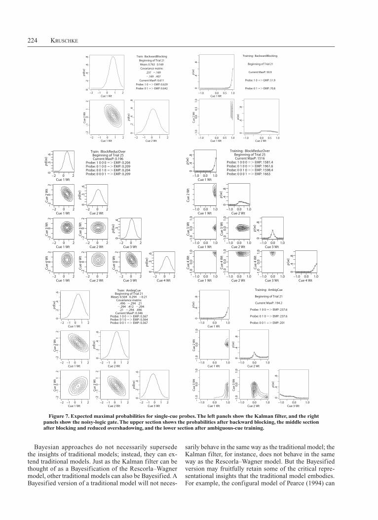
224 KruschKe

sarily behave in the same way as the traditional model; the Kalman filter, for instance, does not behave in the same way as the Rescorla–Wagner model. But the Bayesified version may fruitfully retain some of the critical repre-sentational insights that the traditional model embodies. For example, the configural model of Pearce (1994) can

Bayesian approaches do not necessarily supersede the insights of traditional models; instead, they can ex-tend traditional models. Just as the Kalman filter can be thought of as a Bayesification of the Rescorla–Wagner model, other traditional models can also be Bayesified. A Bayesified version of a traditional model will not neces-

−2 −1 0 1 2Cue 1 Wt

pd

(w)

−2 −1 0 1 2Cue 2 Wt

pd

(w)

Cue 1 Wt

Cu

e 2

Wt

−2 −1 0 1 2

−2

−1

01

2

Train: BackwardBlocking


Mean: 0.763 0.169

Covariance matrix:

.237 �.169

�.169 .407

Current MaxP: 0.611

Probe: 1 0 �� EMP: 0.629

Probe: 0 1 �� EMP: 0.642 0

.4

.8

Cue 1 Wt

p(w

)

Cue 2 Wt

p(w

)

Cue 1 Wt

Cu

e 2

Wt



Current MaxP: 50.9

Probe: 1 0 �� EMP: 51.9

Probe: 0 1 �� EMP: 70.8

−2 0 2

0

.3

.6

Cue 1 Wt

pd

(w)

−2 0 2Cue 2 Wt

pd

(w)

−2 0 2Cue 3 Wt

pd

(w)

−2 0 2Cue 4 Wt

pd

(w)

Cue 1 Wt

Cu

e 2

Wt

−2 0 2

−2

02

Cue 1 Wt

Cu

e 3

Wt

−2 0 2

−2

02

Cue 1 Wt

Cu

e 4

Wt

−2 0 2

−2

02

Cue 2 Wt

Cu

e 3

Wt

−2 0 2

−2

02

Cue 2 Wt

Cu

e 4

Wt

−2 0 2

−2

02

Cue 3 Wt

Cu

e 4

Wt

−2 0 2

−2

02

Train: BlockReducOverBeginning of Trial 25Current MaxP: 0.196

Probe: 1 0 0 0 �� EMP: 0.204Probe: 0 1 0 0 �� EMP: 0.209Probe: 0 0 1 0 �� EMP: 0.204Probe: 0 0 0 1 �� EMP: 0.209 −1.0 0.0 1.0

0

.4

.8

Cue 1 Wt

p(w

)

−1.0 0.0 1.0Cue 2 Wt

p(w

)

−1.0 0.0 1.0Cue 3 Wt

p(w

)

−1.0 0.0 1.0Cue 4 Wt

p(w

)

Cue 1 Wt

Cu

e 2

Wt

−1.0 0.0 1.0

Cue 1 Wt

Cu

e 3

Wt

−1.0 0.0 1.0

Cue 1 Wt

Cu

e 4

Wt

−1.0 0.0 1.0

−1.

0

0.0

1.0

Cue 2 Wt

Cu

e 3

Wt

−1.0 0.0 1.0

Cue 2 Wt

Cu

e 4

Wt

−1.0 0.0 1.0Cue 3 Wt

Cu

e 4

Wt

−1.0 0.0 1.0

Training: BlockReducOverBeginning of Trial 25Current MaxP: 1516

Probe: 1 0 0 0 �� EMP: 1581.4Probe: 0 1 0 0 �� EMP: 1961.6Probe: 0 0 1 0 �� EMP: 1598.4Probe: 0 0 0 1 �� EMP: 1663

−2 −1 0 1 2

0

.

2

.

4

.6

Cue 1 Wt

pd

(w)

−2 −1 0 1 2Cue 2 Wt

pd

(w)

−2 −1 0 1 2Cue 3 Wt

pd

(w)

Cue 1 Wt

Cu

e 2

Wt

−2 −1 0 1 2

−2

−1

01

2

Cue 1 Wt

Cu

e 3

Wt

−2 −1 0 1 2

−2

−1

01

2

Cue 2 Wt

Cu

e 3

Wt

−2 −1 0 1 2

−2

−1

01

2

Train: AmbigCueBeginning of Trial 21

Mean: 0.504 0.294 �0.21Covariance matrix: .496 �.294 .21

�.294 .412 �.294 .21 �.294 .496

Current MaxP: 0.346Probe: 1 0 0 �� EMP: 0.367Probe: 0 1 0 �� EMP: 0.364Probe: 0 0 1 �� EMP: 0.367 −1.0 0.0 1.0

0

.4

.8

Cue 1 Wt

p(w

)

−1.0 0.0 1.0Cue 2 Wt

p(w

)

−1.0 0.0 1.0Cue 3 Wt

p(w

)

Cue 1 Wt

Cu

e 2

Wt

−1.0 0.0 1.0

−1.

0

0.

0

1

.0

Cue 1 Wt

Cu

e 3

Wt

−1.0 0.0 1.0Cue 2 Wt

Cu

e 3

Wt

−1.0 0.0 1.0

Training: AmbigCue


Current MaxP: 194.2

Probe: 1 0 0 �� EMP: 237.6

Probe: 0 1 0 �� EMP: 237.6

Probe: 0 0 1 �� EMP: 201

0

.2

.4

.6

.8

−1.0 0.0 0.5 1.0

−1.0 0.0 0.5 1.0

−1.0 0.0 0.5 1.0

−1.

0

0.0

0.5

1.0

−1.

0

0.0

1.0

−1.

0

0.0

1.0

−1.

0

0.0

1.0

−1.

0

0.0

1.0

−1.

0

0.

0

1

.0

−1.

0

0.

0

1

.0

0

.2

.4

.6

.8

0

.4

.8

0

.3

.6

0

.3

.6

0

.3

.6

0

.4

.8

0

.4

.8

0

.4

.8

0

.

2

.

4

.6

0

.

2

.

4

.6

0

.4

.8

0

.4

.8

Figure 7. expected maximal probabilities for single-cue probes. The left panels show the Kalman filter, and the right panels show the noisy-logic gate. The upper section shows the probabilities after backward blocking, the middle section after blocking and reduced overshadowing, and the lower section after ambiguous-cue training.


framework. Traditional theories emphasized simple asso-ciative weights between cues and outcomes. Connection-ist models continued with this commitment to weighted associations but considered more complex connective architectures. Contemporary and future theories will use a variety of more complex representations to capture a learner’s knowledge. These representations will them-selves be learned according to selection from a hierarchy of possibilities dictated by the theories brought to bear by the learner. The new Bayesian framework demands that a theorist be explicit about what representational options are available to the learner and at just what level of analy-sis the Bayesian learning is assumed to take place.

The Bayesian framework provides a natural launching pad for exploring active learning. Active learners manipu-late and intervene in their world. Future research in asso-ciative learning will investigate active learners, including the costs of information gathering and the benefits of the information learned. As active researchers, we learn about the mind by probing it with experiments that are not too costly, but that we expect to yield results that will strongly influence our beliefs about different theories.

aUThor noTe

For helpful comments on drafts of this article, I thank Rick Hullinger and Ed Wasserman. Additional thanks to Ed Wasserman, John Freeman, and the other organizers of the Spence Fest. Correspondence can be ad-dressed to J. K. Kruschke, Department of Psychological and Brain Sci-ences, Indiana University, 1101 E. 10th St., Bloomington IN 47405-7007 (e-mail: [email protected]; URL: www.indiana.edu/~kruschke/).

reFerences

Akgün, A. E., Byrne, J. C., Lynn, G. S., & Keskin, H. (2007). Orga-nizational unlearning as changes in beliefs and routines in organiza-tions. Journal of Organizational Change Management, 20, 794-812.

Baron, J. (1985). Rationality and intelligence. Cambridge: Cambridge University Press.

Courville, A. C., Daw, N. D., Gordon, G. J., & Touretzky, D. S. (2004). Model uncertainty in classical conditioning. In S. Thrun, L. K. Saul, & B. Schölkopf (Eds.), Advances in neural information pro-cessing systems (Vol. 16, pp. 977-984). Cambridge, MA: MIT Press, Bradford Books.

Courville, A. C., Daw, N. D., & Touretzky, D. S. (2006). Bayesian theories of conditioning in a changing world. Trends in Cognitive Sci-ences, 10, 295-300.

Danks, D., Griffiths, T. L., & Tenenbaum, J. B. (2003). Dynamical causal learning. In S. Becker, S. Thrun, & K. Obermayer (Eds.), Ad-vances in neural information processing systems (Vol. 15, pp. 83-90). Cambridge, MA: MIT Press, Bradford Books.

Dayan, P., Kakade, S., & Montague, P. R. (2000). Learning and selec-tive attention. Nature Neuroscience, 3, 1218-1223.

Deneve, S. (2008). Bayesian spiking neurons II: Learning. Neural Com-putation, 20, 118-145.

Denzler, J., & Brown, C. M. (2002). Information theoretic sensor data selection for active object recognition and state estimation. IEEE Transactions on Pattern Analysis & Machine Intelligence, 24, 145-157.

Doyle, A. C. (1890). The sign of four. London: Spencer Blackett.Goodman, N. D., Tenenbaum, J. B., Feldman, J., & Griffiths, T. L.

(2008). A rational analysis of rule-based concept learning. Cognitive Science, 32, 108-154.

Griffiths, T. L., & Tenenbaum, J. B. (2007). Two proposals for causal grammars. In A. Gopnik & L. Schulz (Eds.), Causal learning: Psy-chology, philosophy, and computation (pp. 323-346). Oxford: Oxford University Press.

Kakade, S., & Dayan, P. (2002). Acquisition and extinction in au-toshaping. Psychological Review, 109, 533-544.

easily be made into a Bayesian model, with two modi-fications that are analogous to the Bayesification of the Rescorla–Wagner model. First, the outcome activation must be made probabilistic instead of deterministic. This can be done by, for example, making the anticipated out-come normally distributed, as in Equation 4. Second, the space of all associative weight combinations must be entertained, with a degree of belief for each weight com-bination. This might be done in the same way as for the Kalman filter, with a normal prior, as in Equation 5. In fact, as long as all of the configural nodes in the model are established from the start of learning, the Bayesified configural model is a Kalman filter model for which the inputs are the configural node activations. As another ex-ample, the context-sensitive elemental model of Wagner (2003) could be Bayesified. The Bayesification would proceed with the same steps as for the configural model; all that would differ would be the coding of the inputs. It remains for future research to determine whether the learning behavior of the Bayesified models would retain the advantages of the original models while encompass-ing new abilities.

As an example of a traditional model that might be Bayesified within a hierarchical framework, consider the model of generalization after discrimination learning pro-posed by Spence (1937). The learner experiences two cue values on a stimulus continuum, simultaneously and side by side. Suppose that the continuum is size, and that the stimulus of size 256 is consistently reinforced and the one of size 160 is not. The question is whether the learner has learned about the specific stimulus sizes or has instead learned the relation that larger stimuli are reinforced. If learners acquire the relation, then if they are tested with a novel pair comprising sizes 409 and 256, they should prefer the larger rather than the smaller stimulus, despite the fact that the smaller one (i.e., 256) was always rein-forced during training. Spence (1937) demonstrated that this apparent transposition of response could instead be explained by stimulus-specific learning, if the excitatory generalization from the reinforced stimulus was broader and stronger than inhibitory generalization from the non-reinforced stimulus. On the other hand, it is obvious that adult humans can learn the fully relational generalization. (Spence [e.g., 1956] was careful, however, not to make claims that his theories applied directly to humans.) A hierarchical Bayesian approach to this issue could have both types of representation—stimulus-specific and rela-tional—available to the learner. As the learner experiences the stimuli, beliefs regarding specific cue values are up-dated, as are beliefs regarding candidate relations among the cue values.

Notice that an active learner would have no problem discerning whether specific stimuli or relative stimuli were reinforced. The learner would simply select stimu-lus pairs that would be maximally informative for reduc-ing uncertainty about the alternative hypotheses. Indeed, one avenue for future research is to investigate relational learning in an active-learning paradigm.

The future of associative learning theory will likely be written in more generalized models in the Bayesian

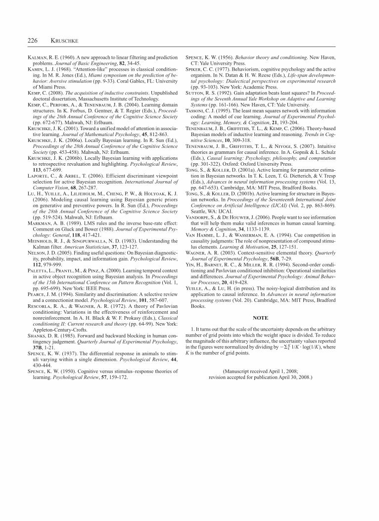
226 KruschKe

Spence, K. W. (1956). Behavior theory and conditioning. New Haven, CT: Yale University Press.

Spiker, C. C. (1977). Behaviorism, cognitive psychology and the active organism. In N. Datan & H. W. Reese (Eds.), Life-span developmen-tal psychology: Dialectical perspectives on experimental research (pp. 93-103). New York: Academic Press.

Sutton, R. S. (1992). Gain adaptation beats least squares? In Proceed-ings of the Seventh Annual Yale Workshop on Adaptive and Learning Systems (pp. 161-166). New Haven, CT: Yale University.

Tassoni, C. J. (1995). The least mean squares network with information coding: A model of cue learning. Journal of Experimental Psychol-ogy: Learning, Memory, & Cognition, 21, 193-204.

Tenenbaum, J. B., Griffiths, T. L., & Kemp, C. (2006). Theory-based Bayesian models of inductive learning and reasoning. Trends in Cog-nitive Sciences, 10, 309-318.

Tenenbaum, J. B., Griffiths, T. L., & Niyogi, S. (2007). Intuitive theories as grammars for causal inference. In A. Gopnik & L. Schulz (Eds.), Causal learning: Psychology, philosophy, and computation (pp. 301-322). Oxford: Oxford University Press.

Tong, S., & Koller, D. (2001a). Active learning for parameter estima-tion in Bayesian networks. In T. K. Leen, T. G. Dietterich, & V. Tresp (Eds.), Advances in neural information processing systems (Vol. 13, pp. 647-653). Cambridge, MA: MIT Press, Bradford Books.

Tong, S., & Koller, D. (2001b). Active learning for structure in Bayes-ian networks. In Proceedings of the Seventeenth International Joint Conference on Artificial Intelligence (IJCAI) (Vol. 2, pp. 863-869). Seattle, WA: IJCAI.

Vandorpe, S., & De Houwer, J. (2006). People want to see information that will help them make valid inferences in human causal learning. Memory & Cognition, 34, 1133-1139.

Van Hamme, L. J., & Wasserman, E. A. (1994). Cue competition in causality judgments: The role of nonpresentation of compound stimu-lus elements. Learning & Motivation, 25, 127-151.

Wagner, A. R. (2003). Context-sensitive elemental theory. Quarterly Journal of Experimental Psychology, 56B, 7-29.

Yin, H., Barnet, R. C., & Miller, R. R. (1994). Second-order condi-tioning and Pavlovian conditioned inhibition: Operational similarities and differences. Journal of Experimental Psychology: Animal Behav-ior Processes, 20, 419-428.

Yuille, A., & Lu, H. (in press). The noisy-logical distribution and its application to causal inference. In Advances in neural information processing systems (Vol. 20). Cambridge, MA: MIT Press, Bradford Books.

noTe

1. It turns out that the scale of the uncertainty depends on the arbitrary number of grid points into which the weight space is divided. To reduce the magnitude of this arbitrary influence, the uncertainty values reported in the figures were normalized by dividing by 2Sk

K 1/K log(1/K), where K is the number of grid points.

(Manuscript received April 1, 2008; revision accepted for publication April 30, 2008.)

Kalman, R. E. (1960). A new approach to linear filtering and prediction problems. Journal of Basic Engineering, 82, 34-45.

Kamin, L. J. (1968). “Attention-like” processes in classical condition-ing. In M. R. Jones (Ed.), Miami symposium on the prediction of be-havior: Aversive stimulation (pp. 9-33). Coral Gables, FL: University of Miami Press.

Kemp, C. (2008). The acquisition of inductive constraints. Unpublished doctoral dissertation, Massachusetts Institute of Technology.

Kemp, C., Perfors, A., & Tenenbaum, J. B. (2004). Learning domain structures. In K. Forbus, D. Gentner, & T. Regier (Eds.), Proceed-ings of the 26th Annual Conference of the Cognitive Science Society (pp. 672-677). Mahwah, NJ: Erlbaum.

Kruschke, J. K. (2001). Toward a unified model of attention in associa-tive learning. Journal of Mathematical Psychology, 45, 812-863.

Kruschke, J. K. (2006a). Locally Bayesian learning. In R. Sun (Ed.), Proceedings of the 28th Annual Conference of the Cognitive Science Society (pp. 453-458). Mahwah, NJ: Erlbaum.

Kruschke, J. K. (2006b). Locally Bayesian learning with applications to retrospective revaluation and highlighting. Psychological Review, 113, 677-699.

Laporte, C., & Arbel, T. (2006). Efficient discriminant viewpoint selection for active Bayesian recognition. International Journal of Computer Vision, 68, 267-287.

Lu, H., Yuille, A., Liljeholm, M., Cheng, P. W., & Holyoak, K. J. (2006). Modeling causal learning using Bayesian generic priors on generative and preventive powers. In R. Sun (Ed.), Proceedings of the 28th Annual Conference of the Cognitive Science Society (pp. 519-524). Mahwah, NJ: Erlbaum.

Markman, A. B. (1989). LMS rules and the inverse base-rate effect: Comment on Gluck and Bower (1988). Journal of Experimental Psy-chology: General, 118, 417-421.

Meinhold, R. J., & Singpurwalla, N. D. (1983). Understanding the Kalman filter. American Statistician, 37, 123-127.

Nelson, J. D. (2005). Finding useful questions: On Bayesian diagnostic-ity, probability, impact, and information gain. Psychological Review, 112, 979-999.

Paletta, L., Prantl, M., & Pinz, A. (2000). Learning temporal context in active object recognition using Bayesian analysis. In Proceedings of the 15th International Conference on Pattern Recognition (Vol. 1, pp. 695-699). New York: IEEE Press.

Pearce, J. M. (1994). Similarity and discrimination: A selective review and a connectionist model. Psychological Review, 101, 587-607.

Rescorla, R. A., & Wagner, A. R. (1972). A theory of Pavlovian conditioning: Variations in the effectiveness of reinforcement and nonreinforcement. In A. H. Black & W. F. Prokasy (Eds.), Classical conditioning II: Current research and theory (pp. 64-99). New York: Appleton-Century-Crofts.

Shanks, D. R. (1985). Forward and backward blocking in human con-tingency judgement. Quarterly Journal of Experimental Psychology, 37B, 1-21.

Spence, K. W. (1937). The differential response in animals to stim-uli varying within a single dimension. Psychological Review, 44, 430-444.

Spence, K. W. (1950). Cognitive versus stimulus–response theories of learning. Psychological Review, 57, 159-172.

bayesian approaches to associative learning: from …kruschke/articles/kruschke2008.pdfbayesian...

Documents