bayesian areal wombling for geographical boundary ...brad/software/lc.proofs.pdfbayesian areal...

UNCORRECTED PROOF

Bayesian Areal Wombling for Geographical

Boundary AnalysisQ2

Haolan Lu, Bradley P. Carlin

Division of Biostatistics, School of Public Health, University of Minnesota, Minneapolis, MN

In the analysis of spatially referenced data, interest often focuses not on prediction of

the spatially indexed variable itself, but on boundary analysis, that is, the determina-

tion of boundaries on the map that separate areas of higher and lower values. Existing

boundary analysis methods are sometimes generically referred to as wombling, after a

foundational article by Womble (1951). When data are available at point level (e.g.,

exact latitude and longitude of disease cases), such boundaries are most naturally ob-

tained by locating the points of steepest ascent or descent on the fitted spatial surface

(Banerjee, Gelfand, and Sirmans 2004). In this article, we propose related methods for

areal data (i.e., data which consist only of sums or averages over geopolitical regions).

Such methods are valuable in determining boundaries for data sets that, perhaps due to

confidentiality concerns, are available only in ecological (aggregated) format, or are

only collected this way (e.g., delivery of health-care or cost information). After a brief

review of existing algorithmic techniques (including that implemented in the com-

mercial software BoundarySeer), we propose a fully model-based framework for

areal wombling, using Bayesian hierarchical models with posterior summaries com-

puted using Markov chain Monte Carlo methods. We explore the suitability of various

existing hierarchical and spatial software packages (notably S-plus and WinBUGS) to

the task, and show the approach’s superiority over existing nonstochastic alternatives,

both in terms of utility and average mean square error behavior. We also illustrate our

methods (as well as the solution of advanced modeling issues such as simultaneous

inference) using colorectal cancer late detection data collected at the county level in

the state of Minnesota.

Background

The analysis and modeling of spatially referenced data sets have occupied statis-

ticians and geographers for decades. Typically, such data consist of variables that

G E A N 6 2 4 B Dispatch: 6.4.05 Journal: GEAN CE: Sujatha

Journal Name Manuscript No. Author Received: No. of pages: 21 PE: HR Op: gsravi

The work of the second author was supported in part by NIH grant 5–R01–ES07750-07, andby NIH grant 1–R01–CA95955–01.Correspondence: Dr Bradley P. Carlin, Division of Biostatistics, School of Public Health,University of Minnesota, Mayo Mail Code 303, Minneapolis, MN 55455-0392e-mail: [email protected]

Submitted: March 12, 2004. Revised version accepted: October 4, 2004.

Geographical Analysis 37 (2005) 265–285 r 2005 The Ohio State University 265

Geographical Analysis ISSN 0016-7363

BWUS GEAN 624.PDF 06-Apr-05 14:31 286030 Bytes 21 PAGES

operator=Ravishankar

UNCORRECTED PROOF

have been observed at different spatial locations, and one seeks models that capture

possible spatial associations among them. Depending upon the nature of spatial

referencing, spatial data are classified as either point-referenced (often called geo-

statistical) or areal (often called lattice). In the former, the spatial locations are

points with known coordinates, such as latitude–longitude or easting–northing

pairs. For the latter, locations are usually geographic regions (such as counties,

census tracts, or zip codes) along with information on the neighborhood structure

(contiguity) of these regions.

Statistical models for spatial data depend upon the nature of the spatial refer-

encing. The role of spatial models for point-referenced data has historically been

the making of predictions and spatial interpolations over the entire domain, while

models for areal data have been used primarily for smoothing raw rate maps to

reveal broad spatial trends. Recently, however, spatial analysts have shown a

growing interest in detecting zones or boundaries that reveal sharp changes in the

values of spatially oriented variables. For example, in contour maps of spatial sur-

faces, regions with highly compact contour lines indicate zones of abrupt change;

significant changes in gradients are observed as one cuts across these contours.

Similarly, for areal data, the boundary separating two regions with drastically dif-

ferent measurements or fitted values is a boundary of abrupt change.

The general problem of identifying zones of abrupt change is known as womb-

ling, after a foundational article by Womble (1951) that discusses the scientific

importance of this problem. Since then, wombling has become a popular technique

among geneticists, demographers, linguists, ecologists, environmental scientists,

and many others in analyzing spatial relationships. Notable articles in this area

include Barbujani, Jacquez, and Ligi (1990), Barbujani, Oden, and Sokal (1989),

Oden et al. (1993), Bocquet-Appel and Bacro (1994), Fortin (1994, 1997), and

Fortin and Drapeau (1995), with Jacquez, Maruca, and Fortin (2000) offering an

excellent recent review. This literature deals primarily with point-referenced data

(regularly or irregularly spaced), often investigating suitable tessellations of the

spatial domain and the appropriate interpolators for approximating the surface.

The field we broadly refer to as ‘‘wombling’’ is also known as barrier analysis or

edge detection in fields such as landscape topography, systematic biology, sociol-

ogy, ecology, and public health. In all of these fields, the research goal is to identify

regional differences across shared boundaries, in order to identify homogenous re-

gions or discover important ‘‘barriers.’’ Ultimately, the underlying influences re-

sponsible for these barriers are typically of greatest scientific interest. For instance,

the genetic study by Sokal and Thompson (1998) locates barriers (areas) over which

genetic flow (population movement, through changing allele frequencies) is re-

duced or stopped.

As with spatial statistical models, wombling approaches must depend upon

whether the data are point-referenced or areal. A significant amount of both meth-

odological and applied research on wombling with point- (or raster-) level data

exists. For example, Bocquet-Appel and Jakobi (1996) used point wombling

Geographical Analysis

266



UNCORRECTED PROOF

analysis to identify the barriers to the spatial diffusion for the demographic transi-

tion in western Europe. Barbujani, Oden, and Sokal (1989) detect a zone of main

discontinuity using an algorithm operating on a local spatial variance statistic.

In studies of human populations, patient confidentiality laws often restrict

available data to counts or rates over geopolitical regions. As such, in this article we

restrict our attention to the areal data case. Areal wombling (also known as polyg-

onal wombling) is not as well-developed in the literature as point or raster womb-

ling, but some notable articles exist. Oden et al. (1993) provide a wombling

algorithm for multivariate categorical data defined on a lattice. The statistic chosen

is the average proportion of category mismatches at each pair of neighboring sites,

with significance relative to an independence or particular spatial null distribution

judged by a randomization test. Csillag et al. (2001) developed a procedure for

characterizing the strength of boundaries examined at neighborhood level. In this

method, a topological or a metric distance d defines a neighborhood of the can-

didate set of polygons (say, pi). A weighted local statistic is attached to each pi. The

difference statistic calculated as the squared difference between any two sets of

polygons’ local statistic and its quantile measure are used as a relative measure of

the distinctiveness of the boundary at the scale of neighborhood size d. Jacquez andGreiling (2003) estimate boundaries of rapid change for colorectal, lung, and breast

cancer incidence in Nassau, Suffolk, and Queens counties in New York.

Several criteria for determining what constitutes a ‘‘barrier’’ have been sug-

gested in previous boundary analysis research. Most researchers select a dissimi-

larity metric (Euclidean distance, squared Euclidean distance, Manhattan distance,

Steinhaus statistics, etc.) to measure the difference in response between the values

at (say) adjacent polygon centroids. An absolute (dissimilarity metrics greater than

C) or relative (dissimilarity metrics in the top k%) threshold then determines which

borders are considered actual barriers, or parts of the boundary.

The relative (top k%) thresholding method for determining boundary elements

(BEs) is easily criticized, since for a given threshold, a fixed number of BEs will

always be found regardless of whether or not the responses separated by the

boundary are statistically different. Jacquez and Maruca (1998) suggest use of both

local and global statistics to determine where statistically significant BEs are, and a

randomization test (with or without spatial constraints) for whether the boundaries

for the entire surface are statistically unusual.

All of the aforementioned areal wombling approaches (like traditional, point-

level wombling itself) appear to be algorithmic, rather than model-based. That is,

they do not involve a probability distribution for the data, and therefore permit

statements about the ‘‘significance’’ of a detected boundary only relative to pre-

determined, often unrealistic null distributions. To remedy this, in this article we

develop a hierarchical statistical modeling framework to perform areal wombling.

Considering the underlying map and its geographical boundaries as our domain,

our Bayesian statistical approach permits direct estimation of the probability that

two geographic regions are separated by the wombled boundary. Our models

Bayesian Areal WomblingQ1 Haolan Lu and Bradley P. Carlin

267



UNCORRECTED PROOF

account for spatial association and permit the borrowing of strength across different

levels of the model hierarchy, accurately estimating quantities that would be in-

estimable using classical approaches.

The remainder of our article is organized as follows. The next section provides

a brief account of existing methods of crisp areal wombling (where each geograph-

ical border is classified as either part or not part of the boundary), as well as our

hierarchical Bayesian alternative. The subsequent section introduces a model-

based approach to fuzzy areal wombling (where now partial membership of a par-

ticular border in the boundary is permitted), illustrating the variety of practical

benefits that accrue. The penultimate section uses simulation to demonstrate the

Bayesian method’s improved performance over the current, more ad hoc methods.

Finally, the last section discusses our findings and suggests directions for further

research.

Crisp areal wombling

Review of existing methods and software

On an areal map, geopolitical borders are usually closed, that is, they completely

partition the study area. They are completely determined from the definition of the

experimental domain and are usually summarized as an adjacency matrix A, where

aij5 1 or 0 depending upon whether regions i and j are adjacent to each other or

not. Another popular representation is to treat the map as a graph with the nodes

representing the regions and edges connecting neighboring nodes.

However, in areal wombling we are interested only in difference boundaries,

which are those borders that separate two adjacent counties having dramatically

different observed response values. Difference boundaries may, in fact, not fully

partition the map, but only indicate regions that greatly differ with respect to the

outcome variable.

As difference boundaries are determined by a response variable that we assume

has a probability distribution, difference boundaries need to be estimated. To be

precise, suppose we have regions i5 1, . . .,N along with the areal adjacency ma-

trix A, and we have observed a response Yi (e.g., a disease count or rate) for the ith

region. Existing areal wombling algorithms assign a boundary likelihood value

(BLV) to each areal boundary using a Euclidean distance metric between neigh-

boring observations. This distance is taken as the dissimilarity metric, calculated for

each pair of adjacent regions. Thus, if i and j are neighbors, the BLV associated with

the edge (i, j) is

Dij ¼ jjYi � Yj jj

where jj � jj is a distance metric. Locations with higher BLVs are more likely to be a

part of a difference boundary, as the variable changes rapidly there.

The wombling literature and attendant software further distinguishes between

crisp and fuzzy wombling. In the former, BLV’s exceeding specified thresholds are


268



UNCORRECTED PROOF

assigned a boundary membership value (BMV) of 1, so the wombled boundary is

fði; jÞ : jjYi � Yj jj > c; i adjacent to jg for some c40. The resulting edges are

called boundary elements. In the latter (fuzzy) case, BMVs can range between 0

and 1 (say, jjYi � Yjjj=maxijfjjYi � Yj jjg) and indicate partial membership in the

boundary. (We note that the use of the word ‘‘fuzzy’’ here does not refer to the

notion of fuzzy logic, but only to the fact that an edge’s membership or nonmem-

bership in the boundary is no longer absolute; see the section on ‘‘Fuzzy areal

wombling’’).

Example: Minnesota colorectal cancer late detection data. As an illustration,

we consider boundary analysis for a data set recording the rate of late detection of

several cancers collected by the Minnesota Cancer Surveillance System (MCSS), a

population-based cancer registry maintained by the Minnesota Department of

Health. The MCSS collects information on geographic location and stage at detec-

tion for colorectal, prostate, lung, and breast cancers. For each county, the late

detection rate is defined as the number of regional or distant case detections di-

vided by the total cases observed, for the years 1995–1997. As higher late detection

rates are indicative of possibly poorer cancer control in a county, a wombled

boundary for this map might help identify barriers separating counties with different

cancer control methods. Such a boundary might also motivate more careful study of

the counties that separate it, in order to identify previously unknown covariates

(population characteristics, dominant employment type, etc.) that explain the

difference.

In this example, we consider ni, the total number of colorectal cancers occur-

ring in county i, and Yi, the number of these that were detected late. To correct for

the differing number of detections (i.e., the total population) in each county, we

womble not on the Y scale, but on the standardized late detection ratio (SLDR)

scale. This is the ratio of observed to expected late detections,

SLDRi ¼Yi

Ei; i ¼ 1; . . . ;N

where the expected counts are computed via internal standardization as Ei ¼ nir ,

where r ¼P

i Yi=P

i ni, the statewide late detection rate.

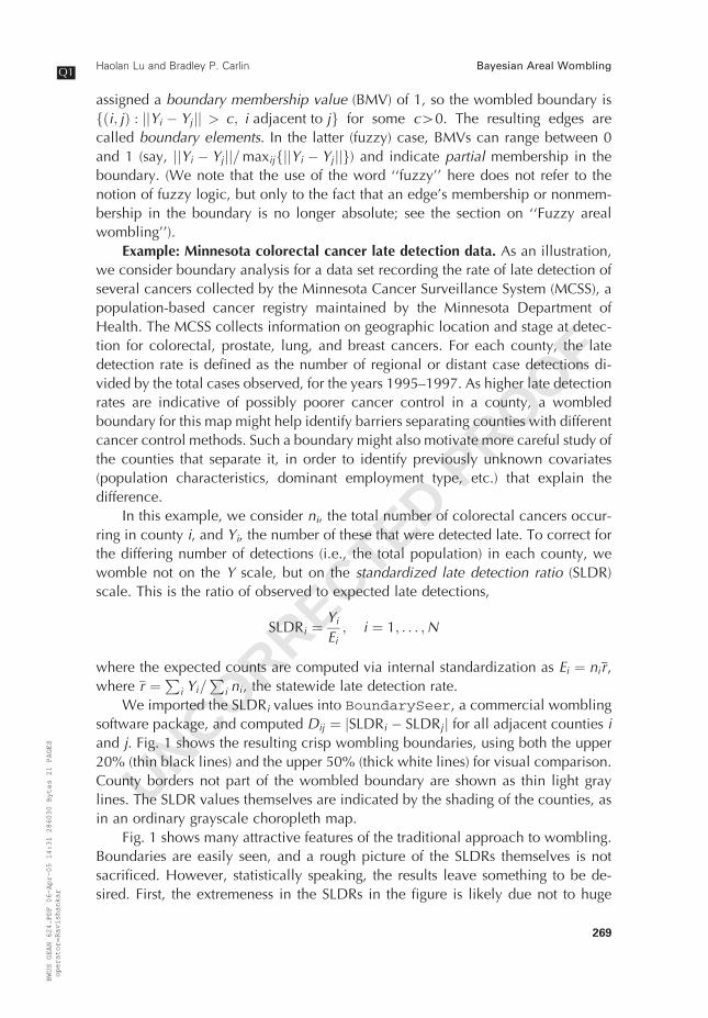
We imported the SLDRi values into BoundarySeer, a commercial wombling

software package, and computed Dij ¼ jSLDRi � SLDRj j for all adjacent counties iand j. Fig. 1 shows the resulting crisp wombling boundaries, using both the upper

20% (thin black lines) and the upper 50% (thick white lines) for visual comparison.

County borders not part of the wombled boundary are shown as thin light gray

lines. The SLDR values themselves are indicated by the shading of the counties, as

in an ordinary grayscale choropleth map.

Fig. 1 shows many attractive features of the traditional approach to wombling.

Boundaries are easily seen, and a rough picture of the SLDRs themselves is not

sacrificed. However, statistically speaking, the results leave something to be de-

sired. First, the extremeness in the SLDRs in the figure is likely due not to huge

Bayesian Areal WomblingQ1

Haolan Lu and Bradley P. Carlin

269



UNCORRECTED PROOF

differences in the true underlying county-level risks, but only to random variation in

the observed data for thinly populated counties. Thus, as already mentioned, we

still require a statistical model for the data in order to properly account for all

sources of uncertainty (both spatial and nonspatial) and enable formal statistical

inference. Second, we need an approach that will smooth the observed data (to

reflect spatial similarity, as well as our differing degrees of confidence in the ob-

served detection rates for urban and rural areas) while simultaneously determining

the boundaries. (Note that a two-step approach applying a standard wombling al-

gorithm to spatially smoothed rates would offer only a partial solution to this sec-

ond goal, as the smoothing and boundary analysis tasks cannot properly be thought

of as independent.)

Hierarchical modeling approach

We now present a statistical modeling framework to rectify the previous subsec-

tion’s omission of both variability and spatial correlation in the response variable Y.

In particular, consider again data having both observed and expected counts (Yi, Ei)

for the ith county. Several authors (e.g., Hodges, Carlin, and Fan 2003) have in-

vestigated areal data models for normal (Gaussian) data, but such models provide

little computational simplification here, and in any case are inappropriate for the

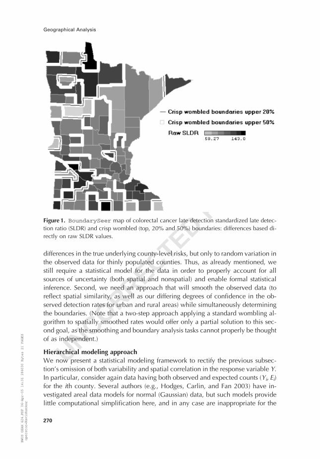
Figure 1. BoundarySeer map of colorectal cancer late detection standardized late detec-

tion ratio (SLDR) and crisp wombled (top, 20% and 50%) boundaries: differences based di-

rectly on raw SLDR values.


270



UNCORRECTED PROOF

count data most commonly encountered in areal settings. As such, we instead em-

ploy the Poisson log-linear form

Yi � PoissonðmiÞ where log mi ¼ log Ei þ x0ibþ fi : ð1Þ

This model allows a vector of region-specific covariates xi (if available), and a

random effect vector /5 (f1, . . .,fN)0 that is given a conditionally autoregressive

(CAR) specification (Besag 1974). A common form of this distribution (often called

the intrinsic CAR, or IAR model) has improper joint distribution, but intuitive con-

ditional distributions of the form

fi j/j 6¼i � Nð�fi ; 1=ðtmiÞÞ ð2Þ

where N denotes the normal distribution, �fi is the average of the /j6¼i that are ad-

jacent to fi, and mi is the number of these adjacencies; this distribution is usually

abbreviated as CAR(t). Finally, t is typically set equal to some fixed value, or as-

signed a distribution itself (usually a relatively vague g distribution).

Markov chain Monte Carlo (MCMC) samples mðgÞi ; g ¼ 1; . . . ;G from the mar-

ginal posterior distribution p(mi|y) can be obtained for each i (see e.g., Banerjee,

Carlin, and Gelfand 2004, Sec. 4.3), from which corresponding samples of the

(theoretical) SLDR,

Zi ¼miEi; i ¼ 1; . . . ;N

are immediately obtained. We may then define the BLV for boundary (i, j) as

Dij ¼ jZi � Zj j for all i adjacent to j ð3Þ

Crisp and fuzzy wombling boundaries are then based upon the posterior dis-

tribution of the BLVs. In the crisp case, we might define ij to be part of the boundary

if and only if E(Dij|y)4c for some constant c40, or if and only if P ðDij � cjyÞ > c�

for some constant 0 < c� < 1.

Model (1)–(2) can be easily implemented in the WinBUGS software package,

freely available from www.mrc-bsu.cam.ac.uk/bugs/welcome.shtml.

WinBUGS includes an easy-to-follow manual and many worked examples; in ad-

dition, www.statslab.cam.ac.uk/ � krice/winbugsthemovie.html

provides a helpful online Flash tutorial. WinBUGS has no limit on N, the number

of areal units. The case of multivariate response variables would require multivari-

ate CAR models (see the concluding section); such models are not yet implemented

in WinBUGS, but could likely be added using the new WinBUGS Development

Interface (WBDev); see the WinBUGS homepage for details.

Posterior draws fZðgÞi ; g ¼ 1; . . . ;Gg and their sample means bEðZijyÞ ¼ 1

G

PGg¼1

ZðgÞi are easily obtained for our problem by mimicking the approach used in the

Scottish lip cancer example (click on ‘‘Map,’’ pull down to ‘‘Manual,’’ and then

click on ‘‘Examples’’), and may then be exported for future use. Bayesian wombling

would naturally obtain posterior draws of the BLVs in (3) by simple transformation



271



UNCORRECTED PROOF

as DðgÞij ¼ jZðgÞ

i � ZðgÞj j, and then base the boundaries on their empirical distribution.

For instance, we might estimate the posterior means as

bEðDijjyÞ ¼1

G

XGg¼1

DðgÞij ¼ 1

G

XGg¼1

jZðgÞi � ZðgÞ

j j ð4Þ

and take as our wombled boundaries the borders corresponding to the top 20% or

50% of these values. A choropleth map of the bEðZi jyÞ then completes a display

similar to Fig. 1.

Unfortunately, BoundarySeer is not designed to permit this sort of analysis,

as it does not expect repeated samples of Dij values to be available. However, we

can ‘‘trick’’ the program into producing what we want by exploiting a feature in-

tended for use with multivariate data. Specifically, suppose we have K random

variables Zki, k5 1, . . .,K observed at each location i. BoundarySeer defines an

omnibus BLV comparing all the variables observed at locations i and j as

Dij ¼XKk¼1

jZki � Zkjj ð5Þ

BoundarySeer refers to this Dij as Manhattan distance, apparently due to its

similarity (when K5 2) to distance as measured by cab drivers in New York City

(city block distance). If we instead use k to index a collection of K Gibbs samples

from p(g|y), then if we set Zki ¼ ZðkÞi , equation (5) delivers exactly K � bEðDijjyÞ. As

K is merely a fixed constant, the wombled boundaries will be unaffected by its

inclusion. The one real limitation here might be that the program currently caps K at

2000, but this should be large enough to deliver sufficient Monte Carlo accuracy inbEðDijjyÞ, provided the sampled ZðgÞi values are not too highly autocorrelated.

Fig. 2 uses thick white lines to show the wombled boundaries arising from the

top 20% of the bEðDijjyÞ values based on this trick using K5G5 1000 Gibbs sam-

ples, superimposed on the fitted colorectal cancer detection true SLDR(Zi) map.

Note there are several differences between the boundaries in this map and the raw

data-based boundaries in Fig. 1. As a side comment, we also experimented with

basing our wombled boundaries only on a subsample of every M Gibbs samples,

where M is chosen large enough so that the subsampled chain is nearly uncorre-

lated. In our case, this meant setting M5 5; the resulting crisp boundaries (not

shown) differ from those shown in Fig. 2 by only two segments.

Hierarchical model selection

Given our analytic goal is the detection of differences between adjacent regions

(i.e., steep gradients in the surface), use of a spatial smoothing model like (2) may

seem odd. It is certainly true that CAR models imply a fairly high degree of smooth-

ing, which may indeed smooth over some apparent boundaries in the raw SLDR

surface. However, the use of raw, unsmoothed measurements may identify bound-


272



UNCORRECTED PROOF

aries that are artificial (say, arising from extreme measurements in two adjacent,

thinly populated regions) rather than real.

As mentioned above, the improper CAR model (2) is often referred to as the

intrinsic CAR, or IAR. Proper versions of the CAR model, as recommended by

Cressie (1993) and others, allow a smaller and, to some extent, data-determined

degree of spatial smoothing. As such, in Table 1 we compare the fit of five models

to our colorectal cancer detection data. Three of these have a single set of random

effects fi: our original IAR, a proper CAR that induces somewhat less spatial

smoothing, and a nonspatial model that assumes the fi to be independent

and identically distributed (i.i.d.) Gaussian white noise random variables. The

Figure 2. Fully Bayesian wombled boundaries based onG51000 Gibbs samples, Boundary

Seer.

Table 1 Goodness-of-Fit D, Effective Model Size pD, and Overall DIC Score for Five Com-

peting Random Effects Models, Minnesota Colorectal Cancer Detection Data

Model D pD DIC

Nonspatial 515.3 50.71 566.0

IAR 511.6 34.63 546.2

Proper CAR 511.6 34.58 546.2

IAR1heterogeneity 520.4 60.82 581.2

Lawson and Clark 518.6 57.83 576.4

DIC, deviance information criterion; CAR, conditionally autoregressive; IAR, intrinsic CAR.



273



UNCORRECTED PROOF

remaining two models have more than one set of random effects. The ‘‘IAR plus

heterogeneity’’ model, popularized byQ3 Besag et al. (1991), replaces the log relative

risk in (1) with

log mi ¼ log Ei þ x0ibþ yi þ fi

where the fi are distributed CAR and the yi are i.i.d. normal. Finally, Lawson and

Clark (2002) propose the mixture model

log mi ¼ log Ei þ x0ibþ yi þ pifi þ ð1� piÞxi ð6Þ

where the yi are again i.i.d. normal, the fi are IAR, the xi are also IAR but under an

L1 (median-based) distance metric, and the pi are weights that trade off between the

spatially smoother fi and the rougher xi, and are such that 0 � pi � 1. While Law-

son and Clark (2002) suggest a symmetric b prior for the pi, we simply set pi5 1/2

for all i, since even with rather informative prior distributions, our data could not

identify the four sets of random effects implied by (6) well enough for our MCMC

algorithm to converge.

While there is disagreement among Bayesians on how best to choose among

competing hierarchical models, the usual penalized likelihood approaches (nota-

bly, AICQ4 and BIC) do not seem sensible here as the theory that supports them does

not extend to the random effects setting. Indeed, it is not even clear how ‘‘big’’ any

of these models are, as their effective size depends on the amount of shrinkage in

the random effects toward each other, and this will be different for every data set.

For instance, the fi in (2) could contribute anywhere from 0 to N effective param-

eters. To settle the issue, Spiegelhalter et al. (2002) recommend use of a deviance

information criterion (DIC) consisting of the sum of a deviance score D and an

effective model size pD. Smaller D values correspond to models that provide better

fit to the data, while smaller pD correspond to more parsimonious models. As there

will often be a tradeoff here (with larger models offering better fit but less parsi-

mony), models with smaller overall DIC scores are to be preferred.

The car.normal, car.proper, and car.L1 distributions in WinBUGS

permit us to fit the five models to the Minnesota colorectal cancer detection data.

The D, pD, and DIC scores in Table 1 were obtained from three independent sam-

pling chains of 10,000 iterations each, following a 1000-iteration burn-in period.

The results indicate that the proper CAR and our original IAR model offer the best

combination of fit and parsimony. The proper CAR gravitates toward a fit nearly as

spatially strong as the IAR: it shares 93% of the IAR’s crisp (upper 20%) wombled

boundaries. The nonspatial model results in a higher effective parameter count, but

not one that improves model fit, and is thus unacceptable. The two multiple ran-

dom effects models similarly do not deliver better fit for their even higher effective

parameter burdens. As the IAR remains slightly more popular in practice than

the proper CAR, in what follows we consider results only for the one-random effect

IAR model.


274



UNCORRECTED PROOF

Comparison of hierarchical and traditional areal wombling

Previously, we noted that BoundarySeer is designed to compute the BLV as the

Manhattan (or other) distance between two region-specific estimates. Taking the

posterior means as these estimates, this leads to basing our wombled boundaries on

D�ij ¼ jbEðZijyÞ � bEðZjjyÞj ð7Þ

instead of bDij � bEðDijjyÞ as given in (4). Hierarchical modeling theory would sug-

gest that boundaries based on bDij (the posterior mean of the absolute difference)

should be superior to those based on D�ij (the absolute difference of the posterior

means), as the former will properly account for uncertainty in the Zi values through-

out the process, rather than averaging this uncertainty out before the BLV is com-

puted. While not a proof of this conjecture, Fig. 3 does indicate that these two sets

of boundaries can be very different: the figure shows histograms of the D�ij and

bDij

values for every potential county boundary segment in the Minnesota colorectal

cancer detection analysis. The latter have a distribution that is far less skewed and

stochastically larger.

As the absolute value function is convex, from Jensen’s inequality we havebDij ¼ EðjZi � ZjjjyÞ � jEðZi � ZjÞjyj ¼ jEðZi jyÞ � EðZjjyÞj ¼ D�ij

and thus the stochastic ordering holds for every segment ij. However, Fig. 3 cannot

reveal whether there is reordering among the potential BLVs that will lead to

Delta-star values

Fre

quen

cy

0 5 10 15 20

0 5 10 15 20

0

10

30

50Top 20%Top 50%

Delta-hat values

Fre

quen

cy

0

20

40

60

80 Top 20%Top 50%

(a)

(b)

Figure 3. Histograms of (a) D�ij and (b) bDij values, Minnesota colorectal cancer detection data,

with upper 50% (dashed) and 20% (solid) cutoffs as indicated.


275



UNCORRECTED PROOF

substantially different wombled boundaries. To check this, Table 2 compares the

pairs of D�ij and

bDij values to see how they match with respect to the upper 20% of

their empirical distributions (the cutoffs for which are marked with solid vertical

lines in Fig. 3). This table reveals that substantial differences do exist that could lead

to different wombled boundaries. We defer more formal comparison of D�ij and

bDij

to the section on ‘‘Simulation study.’’

Fuzzy areal wombling

Traditional approach

Crisp wombled boundaries are easy to comprehend, but their uncertainty is difficult

to assess, as they do not indicate how close to the threshold the mean BLV is, nor

how concentrated its distribution is. Maps of the BLV posterior standard errors can

help somewhat, as can animated sequences of crisp boundaries (see, e.g.,

www.biostat.umn.edu/� haolanl/movie.gif). Still, fuzzy wombled

boundaries may offer a better alternative here, as they do not resort to binary

BMVs. In this subsection, we explore the traditional approach to fuzzy wombling,

and again provide a hierarchical Bayesian version of the procedure.

As mentioned above, fuzzy wombling permits BMVs other than 0 or 1, so that

some areas are allowed to be more important in determining the boundary than

others. Fig. 4 shows how the user may draw this distinction through the choice of

two BLV cutoffs, mt and mc. Specifically, a linear increase in BMV is used between

these two cutoffs, with BMV(BLV5mt)5 0 and BMV(BLV5mc)5 1. Locations

with BLVs below mt are excluded from the boundary, while locations with BLVs

above mc are the ‘‘core’’ boundary (BMV5 1). The mt and mc values may be based

on percentile choices; for example, one can choose mc such that 20% of the BLVs

belong to the core.

To illustrate, Fig. 5 gives a set of fuzzy wombling boundaries for the Minnesota

colorectal cancer detection data drawn in S-plus. Here we have pre-set mc so

that the core boundary contains 20% of all bEðDijjyÞ values, and mt so that the fuzzy

boundary contains the remaining 80% of these values (i.e., every candidate BE is at

least part of the fuzzy boundary). The boundary segments in Fig. 5 are grayscaled so

that the darker the boundary is, the more likely it is above the threshold and thus the

more important it is in determining the boundary.

Hierarchical modeling approach

Traditional fuzzy wombling is appealing in that it avoids a dogmatic 0–1 decision

about whether or not to include a particular map segment in the boundary. The

Table 2 Comparison of the Upper 20% of the Empirical Distributions of D�ij and

bDijbDij not in the upper 20% bDij in the upper 20%

D�ij not in the upper 20% 150 23

D�ij in the upper 20% 23 20


276



UNCORRECTED PROOF

resulting gradations of grayscale in Fig. 5 provide some idea as to how certain we

are that each segment should be included. However, while a fuzzy BMV is between

0 and 1, it may not be interpreted as a ‘‘probability of being part of the boundary,’’

as no stochastic model is associated with the traditional fuzzy algorithm. Yet as-

signing a degree of confidence to each segment is entirely natural, and may well be

the interpretation mistakenly adopted by naive viewers of such plots.

Fortunately, here again the hierarchical Bayesian approach offers a direct and

convenient solution. Suppose we select a cutoff c such that, were we certain a

Figure 4. Illustration of the difference between crisp and fuzzy wombling.

Figure 5. S-plus fuzzy wombling boundaries with grayscale boundary membership values,

Minnesota colorectal cancer detection data.



277



UNCORRECTED PROOF

particular BLV exceeded c, we would also be certain the corresponding segment

was part of the boundary. As our statistical model (1)–(2) delivers the full posterior

distribution of every Dij, we can compute P(Dij4c|y), and take this probability as

our fuzzy BMV for segment ij.

In fact, the availability of the posterior distribution provides another benefit: a

way to directly assess the uncertainty in our fuzzy BMVs. Our Monte Carlo estimate

of P(Dij4c|y) is

bpij � bPðDij > cjyÞ ¼#DðgÞ

ij > c

Gð8Þ

This is nothing but a binomial proportion, where its components independent, ba-

sic binomial theory implies an approximate standard error for it would be

bseðbpijÞ ¼

ffiffiffiffiffiffiffiffiffiffiffiffiffiffiffiffiffiffiffiffiffiffiffibpijð1� bpijÞG

sð9Þ

Of course, our Gibbs samples Dij are not independent in general, as they arise from

a Markov chain, but we can make them approximately so simply by subsampling as

mentioned above, retaining only every Mth sample. Note that this subsampling

does not remove the spatial dependence among the Dij, so repeated use of formula

(9) would not be appropriate if we wanted to make a joint probability statement

involving more than one of the Dij at the same time; we return to this ‘‘simultaneous

inference’’ issue below.

Fig. 6 gives posterior probability areal wombling maps for the Minnesota colo-

rectal cancer detection data using three illustrative values of c (5, 15, and 30), a

subsampling interval of M5 5, and G5 2000. The first row gives boundaries based

on the bpij from equation (8). These three panels show how many and what sort of

boundaries are produced by insisting that the absolute difference in fitted SLDR

between adjacent regions exceed some particular cutoff (5%, 15%, or 30%) with

some probability (indicated by the degree of shading). The second row gives cor-

responding standard error estimates from equation (9). As expected, the probability

of each segment being a member of the boundary decreases as c (the threshold

for being a BE) increases. The bp maps suggest little evidence of strong boundaries

between counties; there are only a few county boundaries estimated to separate

regions with true SLDRs that differ by more than 15%. Still, county 63 (Red Lake, a

T-shaped county in the northwest part of the state) does seem ‘‘isolated’’ from its

two neighbors; again, see a further discussion of this (simultaneous inference)

issue below. The standard error plots reveal that the overall uncertainty associated

with each segment tends to decrease for the more extreme c (5 and 30), as

we become more certain that most segments either are or are not part of the

boundary.

Fig. 7 provides histograms of the fuzzy posterior probability wombled BLVs and

associated standard error estimates given in Fig. 6. The decreasing means are now


278



UNCORRECTED PROOF

much easier to see. Note also thatffiffiffiffiffiffiffiffiffiffiffiffiffiffiffiffi0:25=G

p 0:012 forms an upper bound on the

variance estimates as the formula in (9) has this value as its maximum (obtained

when bpij ¼ 0:5).

An important related point concerns simultaneous inference for a particular

collection of the Dij. Consider again the case of county 63 (Red Lake), which has

counties 57 and 60 as its only neighbors. We may assess whether this county truly is

‘‘isolated’’ from the others by evaluating

~p63 � PðD63;57 > c \ D63;60 > cjyÞ:

As our fDðgÞij g samples come from the joint posterior of D � {Dij}, Monte Carlo

estimates analogous to (8) and (9) are immediately available. The Bayesian ap-

proach thus allows simultaneous inference without reference to the troublesome

frequentist notion of multiple comparisons (which would in turn require Bonferroni

or similar corrections). We could easily repeat this calculation for all ~pi,

i5 1, . . ., 87, perhaps standardizing by the number of segments in each case for

a fairer comparison. Alternatively, we might attempt to consider all pairs of adja-

cent segments on the map, or any predetermined subdivision of the map into pieces

Figure 6. Posterior probability areal wombling for Minnesota colorectal cancer detection

data. First row, wombled boundaries using bpij ; second row, associated estimated standard

errors bseðbpijÞ.



279



UNCORRECTED PROOF

suggested by context (say, a boundary around the Twin Cities metro area, within

which colorectal screening might be hypothesized to be better or more accessible).

We close this section by remarking that wombling on the spatial residuals fi

instead of the fitted SLDRs Zi changes not only the scale of the c cutoff (to difference

in log-relative risk), but the interpretation of the results as well. Specifically, we can

borrow an interpretation often mentioned (but rarely actually used) in spatial ep-

idemiology regarding spatially oriented covariates xi still missing from model (1).

Since boundaries based on the fi separate regions that differ in their unmodeled

spatial heterogeneity, a careful comparison of such regions identified by the wom-

bled map should prove the most fruitful in any missing covariate search. Indeed this

approach should offer a more direct solution than the usual one of searching for

patterns in fitted choropleth disease maps, as it provides a measure of the differ-

ences between regions, rather than the regional levels themselves. On the other

hand, if no significant boundaries exist in the wombled residual map, this is ev-

idence of (covariate-adjusted) mapwide equity, known to public policymakers as

‘‘environmental justice’’ when the response variable measures an environmental

exposure.

p, c=5^F

requ

ency

0.0 0.2 0.4 0.6 0.8 1.0

0

20

40

60

80

0

20

40

60

80

0

20

40

60

80

100

0

20

10

30

40

50

60

0

20

10

30

40

50

60

70

p̂, c=15

Fre

quen

cy0.0 0.2 0.4 0.6 0.8 1.0

p̂, c=30

Fre

quen

cy

0.0 0.2 0.4 0.6 0.8 1.0

se(p̂), c=5

Fre

quen

cy

0.000 0.004 0.008 0.012

se(p̂), c=15

Fre

quen

cy

0.000 0.004 0.008 0.012

se(p̂), c=30

Fre

quen

cy

0.000 0.004 0.008 0.012

0

10

20

30

40

Figure 7. Histograms of posterior wombling probabilities and associated estimated standard

errors, Minnesota colorectal cancer detection data. First row, wombled values for bpij; second

row, associated estimated standard errors bseðbpijÞ.


280



UNCORRECTED PROOF

Simulation study

In this section, we conduct a small simulation study to compare the performance of

D�ij, as given in (7), and bDij, as given in (4). Recall the former is the absolute dif-

ference of the SLDR posterior means, while the latter is the posterior mean of the

absolute difference in the SLDRs. The bDij are more justifiable from a theoretical

point of view, but we might prefer the D�ij if they perform acceptably, since as we

have seen they are computable in BoundarySeer.

Our study proceeds as follows. At iteration k, we first draw a ‘‘true’’ value fðkÞ

� ffðkÞi g from an assumed CAR model, followed by a simulated data vector YðkÞ �

fY ðkÞi g from our Poisson model (1). We then compute the posterior distribution of

the ZðkÞi for each i, hence the posterior summaries D�ðkÞ

ij and bDðkÞij . Averaging over the

R5 216 boundary segments in the Minnesota county map, the mean square errors

(MSEs) of these two estimators relative to the ‘‘truth’’ are

mse�ðkÞ ¼ 1

R

Xi;j

ðD�ðkÞij � DðkÞ

ij Þ2 and dmseðkÞ ¼ 1

R

Xi;j

ðbDðkÞij � DðkÞ

ij Þ2

Finally, averaging these scores over K simulated data sets Y(k) generated in this way,

we would obtain the overall scores mse� and dmse, with smaller numbers of course

indicating better performance.

Our simulations use the same Minnesota county map and adjacency structure

as above, as well as the expected counts Ei from the Minnesota colorectal cancer

detection data set. For convenience we set b5 0 in (1) and t5 1 in (2). However,

the usual CAR prior is improper: note that if the same constant is added to every fi,

fi increases by this same amount, and the probability specification in (2) is un-

changed. This location invariance means it is not immediately obvious how to ob-

tain a single draw from the CAR prior. One solution here is to again use WinBUGS:

We simply run the same code as used for computing the posterior, but after deleting

the Poisson likelihood. WinBUGS adds a ‘‘sum-to-zero’’ constraint (PN

i¼1 fi ¼ 0) by

recentering the fi after every iteration of the Gibbs sampler, resolving the impro-

priety. Iterating over the full conditional distributions in (2), we obtain the desired

CAR draw at ‘‘convergence’’ (say, 100 iterations) of this preliminary sampler.

We considered MSE performance over K5 100 simulated data sets. Obtaining

the K posterior summaries requires repeated use of the WinBUGS language. Such

iteration is possible using within the R programming environment (www.r-project.

org); see www.stat.columbia.edu/ � gelman/bugsR/ or www.biostat.

umn.edu/ � brad/BRugs.html/ for details. We obtained the mse�ðkÞ anddmseðkÞ

values plotted versus k in Fig. 8. The fully Bayesian dmseðkÞ

values are

smaller in all 100 cases. Averaging over the K5100 simulated data sets we obtain

mse� ¼ 307:70 and dmse ¼ 255:66. Thus once again, bD emerges as the better

performer, motivating use of the fully Bayesian approach.



281



UNCORRECTED PROOF

Discussion and future work

In this article, we have presented a model-based approach to areal wombling, using

Bayesian hierarchical models and implemented via Markov chain Monte Carlo

computing methods. The approach enables direct probability statements regarding

the likelihood that a particular geographic border is a boundary, and also correctly

accounts for both spatial and nonspatial uncertainty in the data.

The problem of aggregation bias has been much discussed in the geographical

and spatial statistical literature, and we hasten to add that our Bayesian methods

can fall victim to the same ‘‘ecological fallacy’’ issues that would plague any ag-

gregated data analysis. A complete discussion of this issue is beyond the scope of

this article, but we refer the reader to Banerjee, Carlin, and Gelfand (2004, p. 175)

for more discussion of this problem in the context of hierarchical spatial models.

While in this article we have focused on just a few software packages (Bound-

arySeer, S-plus, and WinBUGS), they are by no means the only ones that might

be used in our context. For example, on the mapping side, the public domain C/

C11 program shapelib can be used to extract polygons from ArcView shape

files for map regions. On the Bayes/MCMC side, our hierarchical models could be

implemented in C/C11, R/S-plus, or Matlab. This last package also includes a

‘‘Spatial Econometrics Toolbox’’ that permits both mapping and MCMC estimation

in a single software environment. In our work, we accomplish this same goal via

an R/S-plus routine (see www.biostat.umn.edu/ � yuecui/) to import

boundaries from ArcView into WinBUGS. We prefer this approach as WinBUGS

0 20 40 60 80 100

200

300

400

500

MS

E

MSE based on ∆*

MSE based on ∆̂

Figure 8. Mean square errors (MSEs) comparison betweenD� and bD over 100 simulated data sets.


282



UNCORRECTED PROOF

permits not only mapping but also automatic generation of the spatial adjacency

matrix.

A strong advantage of our approach is that it uses only standard algorithms and

software, freely available and familiar to working spatial statisticians. However,

future work looks to expanding beyond our current model class in order to allow

even more flexibility. For example, suppose we seek boundaries based on obser-

vations of K41 variables over each region. That is, we now have Yki where k in-

dexes the variable (or ‘‘working map’’). We might assume these Yki were still

independent Poisson random variables as in (1), but where now the /i5 (f1i, . . .,

fKi)0 are assigned amultivariate CAR distribution, generalizing (2); see Gelfand and

Vounatsou (2003), or Banerjee, Gelfand, and Sirmans (2004, Sec. 7.4). Wombling

may now proceed much as before, but with a model that captures correlation both

across space and among the K variables.

Returning to the univariate setting, note that CAR model (2) can be written as

fij/ð�iÞ � N

Pj wijfjPj wij

;1

tP

j wij

!ð10Þ

where the weights wij are equal to 1 if i 6¼j and regions i and j are adjacent, and 0

otherwise. Model (10) remains a valid distributional specification provided

0 � wij � 1, offering a far richer class of possibilities for spatial smoothing. For

example, we might choose the wij inversely proportional to the distance separating

the centroids of regions i and j.

Even more generally, we could think of the wij as additional unknown param-

eters to be estimated, thus allowing the data (and perhaps other observed covariate

information) to help determine the degree and nature of spatial smoothing. For ex-

ample, suppose for all adjacent regions i and j, we follow an idea from statistical

social network analysis (Wang andWong 1987; Hoff, Raftery, and Handcock 2002)

and model the wij as

wijjpij � BernoulliðpijÞ; where logpij

1� pij

� �¼ z0ij c ð11Þ

That is, border segment ij is a BE with probability pij, which in turn arises from a

logit model that depends on a set of boundary-specific covariates zij with corre-

sponding parameter vector c. A wide variety of covariates might be considered

here; for instance, we might set z1ij5 1 (so that g1 is an intercept parameter),

z2ij5 dij, the distance between the centroids of regions i and j, z3ij5 (areai1areaj)/

2, the average area of the two regions, and z4ij5 |xi� xj|, the absolute difference of

some regional covariate (percent urban, percent of residents who are smokers, or

even the region’s expected age-adjusted disease count). Such covariates may arise

without error (as from a census), or with error (as from a survey asking whether

respondents have undergone a colorectal cancer screening procedure within the

last 2 years) that may be acknowledged by adding an errors-in-covariates term to



283



UNCORRECTED PROOF

the model (see, e.g., Xia and Carlin 1998). Reilly (2001) shows that c is estimable

from the data, even under a noninformative prior distribution for c (say, a multi-

variate normal with a vague covariance specification). For g4, say, we would expect

a negative value to emerge, so that regions that are adjacent but have dissimilar

covariate values would be less likely to be considered ‘‘neighbors’’ in the spatial

model. Wombled boundaries might then be based on the posterior distribution of

the Dij as before, or perhaps on the posterior of the wij themselves, as they represent

the extent to which i and j should be thought of as similar or dissimilar. For in-

stance, crisp boundaries could arise as those segments ij having Pðwij ¼ 0jyÞ > c�,

while fuzzy boundaries could use the P(wij5 0|y) values themselves as the BMVs.

As a final, similar but more streamlined generalization, we might delete the pijfrom model (11) and instead place the logit structure directly on the wij, that is,

logwij

1�wij

� �¼ z0ijc for i, j adjacent. The wij will now have distributions (induced by

g0 and g1) residing on the entire interval [0, 1], making their posterior means very

natural fuzzy BMVs.

In summary, advanced areal wombling models of this type offer the potential to

further expand on the aforementioned advantages hierarchical modeling methods

enjoy over traditional approaches to boundary analysis. As spatially referenced

areal data become more and more available in an ever-increasing range of appli-

cation areas, the need to precisely measure and quantify the significance of bound-

aries will exhibit commensurate growth. Our preliminary efforts suggest a bright

future for the merger of statistical methods with geographical analysis tools and

software in this regard.

Acknowledgements

We are grateful to Prof. Sudipto Banerjee and Dr Sally Bushhouse for providing and

permitting analysis of the data sets herein, as well as for helpful discussions that

were essential to this project’s completion.

References

Banerjee, S., B. P. Carlin, and A. E. Gelfand. (2004). Hierarchical Modeling and Analysis for

Spatial Data. Boca Raton, FL: Chapman & Hall/CRC Press.

Banerjee, S., A. E. Gelfand, and C. F. Sirmans. (2004). ‘‘Directional Rates of Change Under

Spatial Process Models.’’ Journal of the American Statistical Association (to appearQ5 ).

Barbujani, G., G. M. Jacquez, and L. Ligi. (1990). ‘‘Diversity of Some Gene Frequencies in

European and Asian populations V. Steep Multilocus Clines.’’ American Journal of

Human Genetics 47, 867–75.

Barbujani, G., N. L. Oden, and R. R. Sokal. (1989). ‘‘Detecting Regions of Abrupt Change in

Maps of Biological Variables.’’ Systematic Zoology 38, 376–89.

Besag, J. (1974). ‘‘Spatial Interaction and the Statistical Analysis of Lattice Systems (with

Discussion).’’ Journal of the Royal Statistical Society, Series B 36, 192–236.

Bocquet-Appel, J. P., and J. N. Bacro. (1994). ‘‘Generalized Wombling.’’ Systematic Biology

43, 442–48.


284



UNCORRECTED PROOF

Bocquet-Appel, J.-P., and L. Jakobi. (1996). ‘‘Barriers for the Spatial Diffusion for the

Demographic Transition in Europe.’’ In Spatial Analysis of Biodemographic Data,

117–29, edited by J. P. Bocquet-Appel, D. Courgeau, and D. Pumain. Londres et Paris,

France: Eurotext, John Libbey.

Cressie, N. A. C. (1993). Statistics for Spatial Data, revised ed. New York: Wiley.

Csillag, F., B. Boots, M.-J. Fortin, K. Lowell, and F. Potvin. (2001). ‘‘Multiscale

Characterization of Boundaries and Landscape Ecological Patterns.’’ Geomatica 55,

291–307.

Fortin, M.-J. (1994). ‘‘Edge Detection Algorithms for Two-Dimensional Ecological Data.’’

Ecology 75, 956–65.

Fortin, M.-J. (1997). ‘‘Effects of Data Types on Vegetation Boundary Delineation.’’ Canadian

Journal of Forest Research 27, 1851–58.

Fortin, M.-J., and P. Drapeau. (1995). ‘‘Delineation of Ecological Boundaries: Comparisons

of Approaches and Significance Tests.’’ Oikos 72, 323–32.

Gelfand, A. E., and P. Vounatsou. (2003). ‘‘Proper Multivariate Conditional Autoregressive

Models for Spatial Data Analysis.’’ Biostatistics 4, 11–25.

Hodges, J. S., B. P. Carlin, and Q. Fan. (2003). ‘‘On the Precision of the Conditionally

Autoregressive Prior in Spatial Models.’’ Biometrics 59, 317–22.

Hoff, P. D., A. E. Raftery, and M. S. Handcock. (2002). ‘‘Latent Space Approaches to Social

Network Analysis.’’ Journal of the American Statistical Association 97, 1090–98.

Jacquez, G. M., and D. A. Greiling. (2003). ‘‘Geographic Boundaries in Breast, Lung and

Colorectal Cancers in Relation to Exposure to air Toxics in Long Island, New York.’’

International Journal of Health Geographics 2, 4.

Jacquez, G. M., and S. L. Maruca. (1998). ‘‘Geographic Boundary Detection.’’ In

Proceedings of the 8th International Symposium on Spatial Data Handling, edited by T.

K. Poiker and N. Chrisman. Burnaby, BC, Canada: International Geographic Union,

Geographic Information Science Study Group.

Jacquez, G. M., S. Maruca, and M.-J. Fortin. (2000). ‘‘From Fields to Objects: A Review of

Geographic Boundary Analysis.’’ Journal of Geographical Systems 2, 221–41.

Lawson, A. B., and A. Clark. (2002). ‘‘Spatial Mixture Relative Risk Models Applied to

Disease Mapping.’’ Statistics in Medicine 21, 359–70.

Oden, N. L., R. R. Sokal, M.-J. Fortin, and H. Goebl. (1993). ‘‘Categorical Wombling:

Detecting Regions of Significant Change in Spatially Located Categorical Variables.’’

Geographical Analysis 25, 315–36.

Reilly, C. (2001). ‘‘Modeling Adjacency in Lattice Models.’’ Research Report, Division of

Biostatistics, University of Minnesota.

Sokal, R. R., and B. A. Thompson. (1998). ‘‘Spatial Genetic Structure of Human Populations

in Japan.’’ Human Biology 70, 1–22.

Spiegelhalter, D. J., N. Best, B. P. Carlin, and A. van der Linde. (2002). ‘‘Bayesian Measures

of Model Complexity and Fit (With Discussion).’’ Journal of the Royal Statistical Society,

Series B 64, 583–639.

Wang, Y. J., and G. Y. Wong. (1987). ‘‘Stochastic Blockmodels for Directed Graphs.’’ Journal

of the American Statistical Association 82, 8–19.

Womble, W. (1951). ‘‘Differential Systematics.’’ Science 114, 315–22.

Xia, H., and B. P. Carlin. (1998). ‘‘Spatio-Temporal Models with Errors in Covariates:

Mapping Ohio Lung Cancer Mortality.’’ Statistics in Medicine 17, 2025–43.


285



GEAN

624

1. Disk Usage :- Disk not provided

Disk used Disk not used

Disk is corruptUnknown file formatVirus found

Additional Work done:

¨

¨ ¨

¨¨¨

¨

þ

Author ResponseDescriptionQueryNo.

2. Queries :-

While preparing this paper/manuscript for typesetting, the following queries have arisen.

Journal

Article

Author Query Form

AQ: Please check if the suggested running title is OK.Q1

Production Editor: Please confirm that the deletion of designations, etc, (graduate assistant and MayoProfessor) is OK. If to be retained, please provide the format/style (as footnotes to the authors)?

Q2

AQ: Besag et al. (1991) has not been included in the list, please include and supply publication details.Q3

AQ: Please expand AIC and BIC.Q4

AQ: Please provide volume number and pagerange for Banerjee et al. (2004).Q5

figures 5 and 6 appears to be incomplete please check

bayesian areal wombling for geographical boundary ...brad/software/lc.proofs.pdfbayesian areal...

Documents