bayesian calibration of models - cmu › pozzi › files › 2015 › 09 ›...

Lec. 0712735: Urban Systems Modeling Bayesian model calibration

12735: Urban Systems Modeling

instructor: Matteo Pozzi

1

Bayesian calibration of models

Lec. 07


outline

2

‐ Intro on model calibration;

‐ log‐likelihood, maximum likelihood estimator;

‐ Bayesian approach, Metropolis algorithm to calibration;

‐ application to extreme precipitations


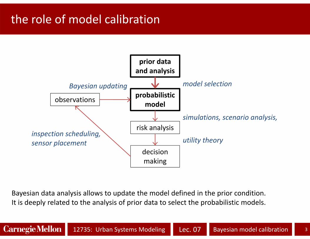
the role of model calibration

3

prior data and analysis

probabilistic model

risk analysis

decision making

observations

utility theory

Bayesian updating

simulations, scenario analysis,

model selection

inspection scheduling,sensor placement

Bayesian data analysis allows to update the model defined in the prior condition.It is deeply related to the analysis of prior data to select the probabilistic models.


-2 0 2 4 6 8 10

0

0.05

0.1

0.15

0.2

0.25

p xN = 200

-2 0 2 4 6 8 10x

calibrating probabilistic models

4

problem statement: given set , identify distribution so that

~

approach: let us select a parametric form for : , so to identify is to select a value for . , ,

-2 0 2 4 6 8 10

0

0.05

0.1

0.15

0.2

0.25

p xN = 200

-2 0 2 4 6 8 10x


-2 0 2 4 6 8 10

0

0.5

1

F x

moment matching and curve fitting

5

moment matching: compute sample moments and the corresponding exact moments as a function of . Derive : Momement ≡SampleMoments.

-2 0 2 4 6 8 10

0

0.05

0.1

0.15

0.2

0.25

p xN = 200

-2 0 2 4 6 8 10x

: # of parameters

curve fitting: identify that gives best fitting between empirical and exact PDF (or CDF).


calibrating probabilistic models: LH and MLE

6

likelihood function: agreement between dataset and parameters.∏ with dataset

maximum likelihood estimator: argmax optimization

-2 0 2 4 6 8 10

0

0.05

0.1

0.15

0.2

0.25

p xN = 200

-2 0 2 4 6 8 10x

independent samples, as for independent measures measures as samples

estimated model:


-2 0 2 4 6 8 10

-7

-6

-5

-4

-3

-2

-1lo

g ( p

x )N = 20

-2 0 2 4 6 8 10x

log‐LH

7


independent samples, as for independent measures

log ∑ log mean log ∝ mean log

∃ : 0 ⇒ mean log ∞ 0

log‐norm. models are incompatible with data


Bayesian inference on probabilistic models

8


prior: inference: →

-2 0 2 4 6 8 10

0

0.05

0.1

0.15

0.2

0.25

p xN = 200

-2 0 2 4 6 8 10x

estimated model:

historic dataset

new outcome

to be predicted


toy example: Gaussian linear model

9

Normal model with known variance ( | ), and unknown mean ( | ):, | , |

likelihood:∏ ∏ , | , | ∝

, | , | / , , | /

∑ sample mean

normal prior:, ,

posterior: , | , |

predictions:

, | , | |

MLE: → , , |

| , | : from GLM formulas

combining uncertainty in inference and in prediction


processing extreme precipitation data

10

climate model: HADCM3 outcome: average rain intensity on 3 hours average, every 3 hours, for period 1968‐2000, 2037‐2069.data are available at a 50 50km2 grid.

annual maxima for some durations (3h, 6h, 12h, 24h, 48h) are derived by moving average.

1000 2000 3000 4000 5000 6000 7000 80000

5

10

15

t [h]

I [m

m/h

]

year = 1977

with Sham Thanekar, Peter Adams



11

task: model annual maximum of rain intensitygiven , with the maximum at year , identify so that ~

interpretation: each annual maximum is sampled independently from .

1970 1980 1990 2000 2010 2020 2030 2040 2050 2060 2070

100

101

year

I [m

m/h

]

3h6h12h24h48h



12

task: model annual maximum of rain intensitygiven , with the maximum at year , identify so that ~

interpretation: each annual maximum is sampled independently from .

1970 1980 1990 2000 2010 2020 2030 2040 2050 2060 2070

100

101

year

I [m

m/h

]

3h6h12h24h48h

0 1 2

px


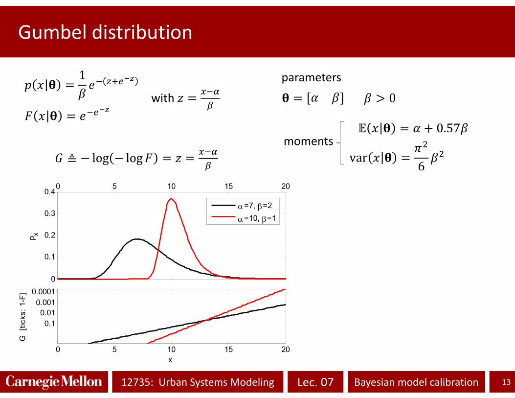
Gumbel distribution

13

1

with

parameters

0

0.57

var 6

moments≜ log log

0 5 10 15 20

0

0.1

0.2

0.3

0.4

p x

0 5 10 15 20

0.10.01

0.0010.0001

x

G [

ticks

: 1-F

]

=7, =2

=10, =1


inference using Gumbel: log‐LH

14

log log ∑ with

log(LH)

5 6 7 8 9 101

1.5

2

2.5

3

3.5

4

4.5

5

0 5 10 15 20

0

0.05

0.1

0.15

0.2

p x

dataset=7.5, =2.5=9, =3.5

0 5 10 15 20x

mm/h

as usual, MLE can be identified by solving an optimization problem.


inference using Gumbel: Metropolis’ algorithm

15

log log ∑ with

prior: : ~ ~ inference: →

5 6 7 8 9 10

1

1.5

2

2.5

3

3.5

4

4.5

5

0 500 1000 1500 20002

3

4

5

6

7

8

9

10

# of sim.

,

rejection rate = 40%

starting pointMetropolis’ algorithm: random steps.


2 4 6 8 10 12 14 16 18

0

0.05

0.1

0.15

0.2

p x

0.1

0.01

G [t

icks

: 1-F

]

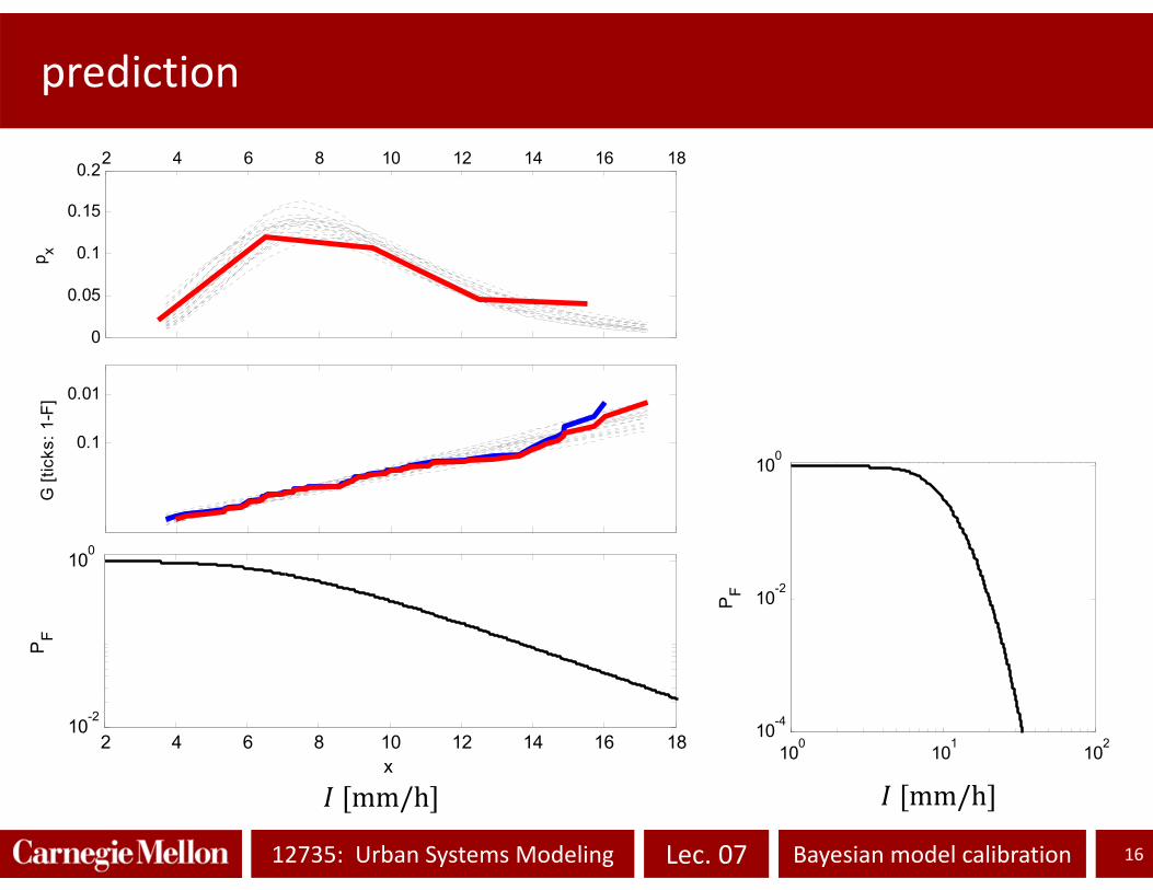
prediction

16

mm/h

2 4 6 8 10 12 14 16 1810-2

100

x

PF

100 101 10210-4

10-2

100

PF

mm/h


return period

17

100 101 10210-4

10-2

100

PF

mm/h

define threshold ∗: failure F if annual maximum is above ∗. Safe S otherwise.≜ ℙ F ℙ ∗ 1 ∗ . 0 1

realization: SSSSFSSSSSSSSSFSSSS…

Δ1

ifΔ 1ifΔ 2

1⋮

ifΔ 3⋮

Δ: number of years before next failure: it is a random variable123456789…

Δ 5

∀ ∈ , Δ 1

≜ Δ ∗

∗ 1intensity (function of return period)

Bernoulli process: every year failure occurs with probability .

geometrical distribution

return period


how to build intensity duration frequency curves

18

Fix return period (frequency), selected duration ( ), derive intensity ∗ 1 .

http://hdsc.nws.noaa.gov/


time trend: parameters change with time

19

1970 1980 1990 2000 2010 2020 2030 2040 2050 2060 2070

101

time [year]

x Lim

:

I [m

m/h

]

T=5yT=10yT=20yT=50yT=100yT=500y

1

logwith

parameters

log log

log ∑ log with


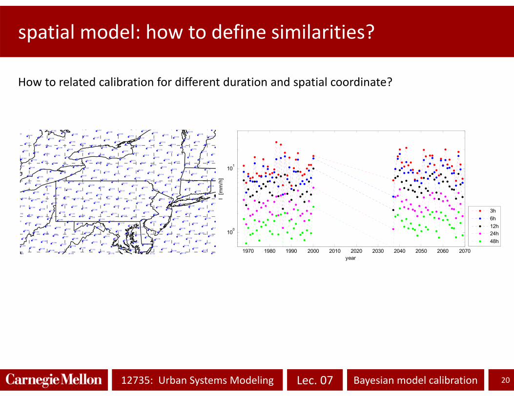
spatial model: how to define similarities?

20

How to related calibration for different duration and spatial coordinate?

1970 1980 1990 2000 2010 2020 2030 2040 2050 2060 2070

100

101

year

I [m

m/h

]

3h6h12h24h48h

bayesian calibration of models - cmu › pozzi › files › 2015 › 09 ›...

Documents