bayesian decision making in groups is hard
TRANSCRIPT
Bayesian Decision Making in Groups is HardJan Hązła1,2, Ali Jadbabaie1,3, Elchanan Mossel1,2, M. Amin Rahimian1
1Institute for Data, Systems and Society 2Department of Mathematics 3Laboratory for Information and Decision SystemsMassachusetts Institute of Technology
jhazla,jadbabai,elmos,[email protected]
We study the computations that Bayesian agents undertake when exchanging opinions over a network. The
agents act repeatedly on their private information and take myopic actions that maximize their expected
utility according to a fully rational posterior belief. We show that such computations are NP-hard for two
natural utility functions: one with binary actions, and another where agents reveal their posterior beliefs. In
fact, we show that distinguishing between posteriors that are concentrated on different states of the world is
NP-hard. Therefore, even approximating the Bayesian posterior beliefs is hard. We also describe a natural
search algorithm to compute agents’ actions, which we call elimination of impossible signals, and show that
if the network is transitive, the algorithm can be modified to run in polynomial time.
Key words : Observational Learning, Bayesian Decision Theory, Computational Complexity, Group
Decision-Making, Computational Social Choice, Inference over Graphs
MSC2000 subject classification : Primary: 91B06; secondary: 68Q25, 91A35, 62C10
OR/MS subject classification : Primary: Games/group decisions: Voting/committees; secondary:
Organizational studies: Decision making Effectiveness/performance Information; Networks/graphs
JEL: D83, D85.
Working paper. July 27, 2019. Authors are listed in alphabetic order.
1. Introduction
Many decision-making problems involve interactions among individuals (agents) exchanging infor-
mation with each other and striving to form rational opinions. Such situations arise in jury delibera-
tions, expert committees, medical diagnoses, etc. Given their many important applications, relevant
models of decision making in groups have been extensively considered over the years.
The first interesting case concerns only two agents. A fundamental insight offered by Aumann
(1976) indicates that having common priors and a common knowledge of posterior beliefs imply
agreement: Rational agents cannot agree to disagree. Later work by Geanakoplos and Polemarchakis
(1982) demonstrates that such an agreement can be achieved in finite time, by broadcasting pos-
terior beliefs back and forth. Banerjee (1992) and Bikhchandani et al. (1998) study the sequential
interaction where each agent observes the decisions of everyone before her. Acemoglu et al. (2011)
1
2 Hązła et al. Bayesian Decision Making in Groups is Hard
extend the sequential learning model to a network environment where agents only observe actions of
their neighbors (rather than all preceding actions). Gale and Kariv (2003) consider repeated (rather
than sequential) interactions over social networks where agents update their beliefs after observing
actions of each other. Following on, a large body of literature studies different aspects of rational
opinion exchange, in particular the quality of information aggregation and learning in the limit (cf.
Acemoglu and Ozdaglar (2011), Mossel and Tamuz (2017) for two surveys of known results).
Another prominent approach to the study of social learning is to model non-Bayesian agents who
use simpler, heuristic rules. One reason for considering non-Bayesian heuristics (so called “bounded
rationality”) in place of fully rational updates is seeming intractability of Bayesian calculations:
Information from different neighbors can exhibit complex correlations, with no obvious way to
account for, and remove them. For example, a Bayesian agent may have to account for the fact that
her neighbors are influenced by the same source of information or even her own past actions (Eyster
and Rabin 2014, Krishnamurthy and Hoiles 2014).
Even though hardness of Bayesian computations in networked, learning models seems to be widely
believed, we are not aware of any previous work making a rigorous argument for it. Our present
work addresses this gap. We analyze algorithmic and complexity theoretic foundations of Bayesian
social learning in two natural environments that are commonly studied in the literature. In one of
them the actions broadcast by agents are coarse, in the sense that they are single bits. In the other
one, we assume that the actions are rich, consisting of agents’ full posterior beliefs. We show that
the computations of the agents are intractable in both cases.
1.1. Our contributions
We analyze a fairly well-studied model of Bayesian social learning. In this model there is a random
variable θ which represents the unknown state of the world and determines payoffs from different
actions. A network of agents receive private signals which are independent conditioned on the value
of θ. At every step t = 0,1,2, . . ., each agent outputs an action ai,t that maximizes her utility
according to her current posterior distribution of θ. The action is chosen myopically, i.e., only utility
at the current time is considered and the posterior µi,t is computed using Bayes rule. Agents learn
actions of their neighbors on the network and proceed to the next step with updated posteriors.
For our hardness results, we study two natural variants of this model. First, we consider the case
of binary actions, where the state, signals and actions are all binary, and each agent outputs the
guess for the state θ ∈ 0,1 that is most likely according to her current belief. This model can be
thought of as repeated voting (e.g., during jury deliberations or the papal conclave in the Catholic
Church). We are interested in the complexity of computations for producing Bayesian posterior

Hązła et al. Bayesian Decision Making in Groups is Hard 3
beliefs µi,t or action ai,t. We also study the revealed belief model where the utilities induce agents
to reveal their current posteriors, or beliefs.
Following the detailed model description in Section 2, we present our complexity results in Sec-
tion 3. We show that it is NP-hard for the agents to compute their actions, both in the binary
action and the revealed belief model. As a common tool in computational complexity theory, NP-
hardness provides rigorous evidence of worst-case intractability. Note that we only prove existence
of intractable network structures and private signals, not that they are “common” or “likely to arise”.
Also, our reductions critically rely on the network structure: They do not apply to sequential models
like the one in Banerjee (1992). One might suspect that the beliefs can be efficiently approximated,
even if they are difficult to compute exactly. This is unfortunately not the case, and we further
prove a hardness-of-approximation result: It is difficult even to distinguish between posterior beliefs
that concentrate almost all of probability on one state and those that are concentrated on another
state. In Section 3 we discuss in more detail what substantive economic assumptions are important
in deriving our complexity results and some ways in which those results can be extended.
In Section 4, we study algorithms for Bayesian decision making in groups and describe a nat-
ural search algorithm to compute agents’ actions. The Bayesian calculations are formalized as an
algorithm for elimination of impossible signals (EIS), whereby the agent refines her knowledge by
eliminating all profiles of private signals that are inconsistent with her observations. In Subsection
4.1, we present recursive and iterative implementations of this algorithm. While the search over the
possible signal profiles using this algorithm runs in exponential time, these calculations simplify in
certain network structures. In Subsections 4.2 and 4.3, we give examples of efficient algorithms for
such cases. As a side result, we provide a partial answer to one of the questions raised by Mossel
and Tamuz (2013), who provide an efficient algorithm for computing the Bayesian binary actions
in a complete graph: We show that efficient computation is possible for other graphs that have
a transitive structure when the action space is finite. In such transitive networks, every neighbor
of a neighbor of an agent is also her neighbor and therefore there are no indirect interactions to
complicate the Bayesian inference.
1.2. Related work
Our results are related to the line of work that studies conditions for consensus and learning among
rational agents (Mossel et al. 2018, Mueller-Frank 2013, Smith and Sørensen 2000). Consensus refers
to all agents converging in their actions or belief (cf. Gale and Kariv (2003), Rosenberg et al. (2009)
for consensus conditions in the network model that we study). Learning means that the consensus
action is efficient, i.e., it represents the state of the world with high probability. For example,
Mossel et al. (2014, 2015) consider the binary action model (for myopic and forward-looking agents,
4 Hązła et al. Bayesian Decision Making in Groups is Hard
respectively) and provide sufficient conditions for learning. These conditions are imposed on the
network structure and consist of bounded out-degree and an “egalitarian” connectivity, whereby if
an agent i observes agent j, there is a reverse path from j to i of bounded length (this condition is
trivially satisfied for undirected networks).
On the other hand, positive computational results for Bayesian opinion exchange (including the
analysis of short-run dynamics) are restricted to small networks (e.g., with three agents (Gale and
Kariv 2003, Section 5), see also examples in Rosenberg et al. (2009)) or special cases. The case of
jointly Gaussian signals and beliefs exhibits a linear-algebraic structure that allows for tractable
computations (Mossel et al. (2016), see also DeMarzo et al. (2003)). Dasaratha et al. (2018) extend
this setup to dynamic state spaces and private signals. There are also efficient algorithms for special
network structures, e.g., complete graphs and trees (Kanoria and Tamuz 2013, Mossel and Tamuz
2013). Moreover, recursive techniques have been applied to analyze Bayesian decision problems with
partial success, Harel et al. (2014), Kanoria and Tamuz (2013), Mossel et al. (2016, 2014) and we
also contribute to this literature by offering new cases where Bayesian decision making is tractable
(cf. Subsections 4.2 and 4.3). This state of affairs might have to do with our computational hardness
results.
Other ways to achieve positive computational results are through alternative communication
strategies or using non-Bayesian information exchange protocols. For example, Acemoglu et al.
(2014) analyze social learning among agents who directly communicate their entire information (rep-
resented as pairs of private signals and their sources). Since each piece of information is tagged, there
is no confounding, and Bayesian updating is simple. On the other hand, the exchanged information
has a significantly more complex form. In contrast, we think of our model as relevant to situations
where, as is often the case, it is not practical to exhaustively list all of one’s evidence and reasoning
instead of stating or summarizing one’s opinion. A popular approach to study bounded rationality
is by replacing Bayesian actions with heuristic (non-Bayesian) rules (Arieli et al. 2019a,b, Bala and
Goyal 1998, DeGroot 1974, Golub and Jackson 2010, Jadbabaie et al. 2012, Li and Tan 2018, Molavi
et al. 2018, Mueller-Frank and Neri 2017). These rules are often rooted in empirically observed
behavioral and cognitive biases. For example, Li and Tan (2018) consider a class of naive agents
who take Bayesian actions but as if their local neighborhood is the entire network. This assumption
removes the possibility of indirect interactions and, similar to the transitive structures (Subsection
4.2), simplifies Bayesian computations. Our work is orthogonal and complementary to these studies.
We prove that Bayesian reasoning is otherwise, in general, computationally intractable (because of
the difficulty of delineating confounded sources of information).
There are also works that focus on two agents estimating an arbitrary random variable (Aaronson
2005) — this is in contrast to our model where the state of the world is correlated with the private
Hązła et al. Bayesian Decision Making in Groups is Hard 5
signals in a simple way. The computational result of Aaronson (2005) concerns a protocol where
the two agents keep exchanging their Bayesian posteriors with a deliberately added noise term. One
might question how “Bayesian” such a protocol is, since the agents are not maximizing a utility
function. On the other hand, the error terms can be reinterpreted as transmission noise or computa-
tion errors of rational agents (where the agents have common knowledge of the noise distribution).
Aaronson (2005) shows that this protocol can be efficiently implemented (approximately and on
average with respect to private signals) for any constant number of rounds. As far as we can see, the
proof of Aaronson (2005) does not extend to many agents and networks. In Subsection 3.6, we show
how to adapt our hardness reduction to this noisy action setting. Notwithstanding, we cannot logi-
cally exclude the possibility of a result like Aaronson (2005), since we show only worst-case hardness
and the algorithm in Aaronson (2005) works on average. Therefore, we leave it as an interesting
open problem: In the network model with noise, does there exist an average-case efficient algorithm,
or are computations hard on average (at least with respect to private signal profiles)?
In fact, our results can be also interpreted in the context of other works pointing at computational
reasons for why economic or sociological models fail to accurately reflect reality (cf., e.g., Arora
et al. (2011) on the computational complexity of financial derivatives and Velupillai (2000) on the
computable foundations of economics). On the one hand, a model cannot be considered plausible
if it requires the participants or agents to perform computations that need a prohibitively long
time. On the other hand, the predictions of such a model can be rendered inaccessible by the
computational barriers. The literature on computational hardness of Bayesian reasoning in social
networks is nascent. There are some hardness results in the literature on Bayesian inference in
graphical models (see Kwisthout (2011) and references therein), but these are quite different from
models considered in this work. Papadimitriou and Tsitsiklis (1987) consider partially observed
Markov decision processes (POMDP). These Markovian processes are not directly comparable to our
model, but they exhibit similar flavor in so far as repeated interactions are concerned. Papadimitriou
and Tsitsiklis (1987) prove that computing optimal expected utility in a POMDP is PSPACE-
hard, achieving a stronger notion of hardness than NP-hardness. However, their result does not
extend to hardness of approximation, i.e., they only show that it is hard to decide if the optimal
agent’s strategy achieves positive (but possibly very small) expected utility. Moreover, the setup for
Bayesian decision making in groups is different (arguably less general, i.e., more challenging for a
hardness proof) than a POMDP. Subsequently, we need different techniques for our purposes.
We also point out a follow-up work by the authors of this paper (Hązła et al. 2019), where we use
significantly more technical arguments to show that the computations in the binary action model are
also (worst case) PSPACE-hard to approximate. We believe the details of the latter work might be
of interest to complexity theorists. Here, we focus on developing more general arguments to inform
operations research and social learning applications.
6 Hązła et al. Bayesian Decision Making in Groups is Hard
2. The Bayesian Group Decision Model
We consider a finite group of agents, whose interactions are represented by a fixed directed graph
G. For each agent i in G, Ni denotes her neighborhood: The subset of agents whose actions are
observed by agent i. Without loss of generality, we will assume that i ∈ Ni, i.e., an agent always
observes herself.
We model the topic of the discussion/group decision process by a state θ belonging to a finite set
Θ. For example, in the course of a political debate, Θ can be the set of all political parties with θ
representing the party that is most likely to increase society’s welfare. The value of θ is not known
to the agents, but they all start with a common prior belief about it, which is a distribution with
probability mass function ν(·) : Θ→ [0,1].
Initially, each agent i receives a private signal si, correlated with the state θ. The private signal si
belongs to a finite set Si and its distribution conditioned on θ is denoted by Pi,θ(·), which is referred
to as the signal structure of agent i. Conditioned on the state θ, the signals si are independent
across agents, and we use Pθ(·) =∏i Pi,θ(·) to denote their joint product distribution.
After receiving the signals, the agents interact repeatedly, in discrete times t= 0,1,2, . . .. Asso-
ciated with every agent i is an action space Ai that represents the choices available to her at any
time t ∈ N0, and a utility ui(·, ·) : Ai × Θ→ R which represents her preferences with respect to
combinations of actions and states. At every time t ∈ N, agent i takes action ai,t that maximizes
her expected utility based on her observation history hi,t:
ai,t = arg maxai∈Ai
E[ui(ai, θ) | hi,t], (1)
where the history hi,t is defined as si ∪ aj,τ for all j ∈Ni, and τ < t, i.e., agent i observes her
private signal, as well as actions of all her neighbors at times strictly less than t.
The network, signal structures, action spaces and utilities, as well as the prior, are all common
knowledge among the agents. We use the notation arg maxa∈A to include the following, common
knowledge, rule when the maximizer is not unique: We assume that the action spaces are (arbitrarily)
ordered and an agent will break ties by choosing the lowest-ranked action in her ordering. The
specific tie-breaking rule is not important for our results. The agents’ behavior is myopic in that it
does not take into account strategic considerations about future rounds; cf. Subsection 3.2.
We denote the Bayesian posterior belief of agent i given her history of observations by its proba-
bility mass function µi,t(·) : Θ→ [0,1]. In this notation, the expectation in (1) is taken with respect
to the Bayesian posterior belief µi,t.
To sum up, agent i at time t chooses an action ai,t ∈Ai, maximizing her expected utility condi-
tioned on the observation history hi,t. Then, she observes the most recent actions of her neighbors
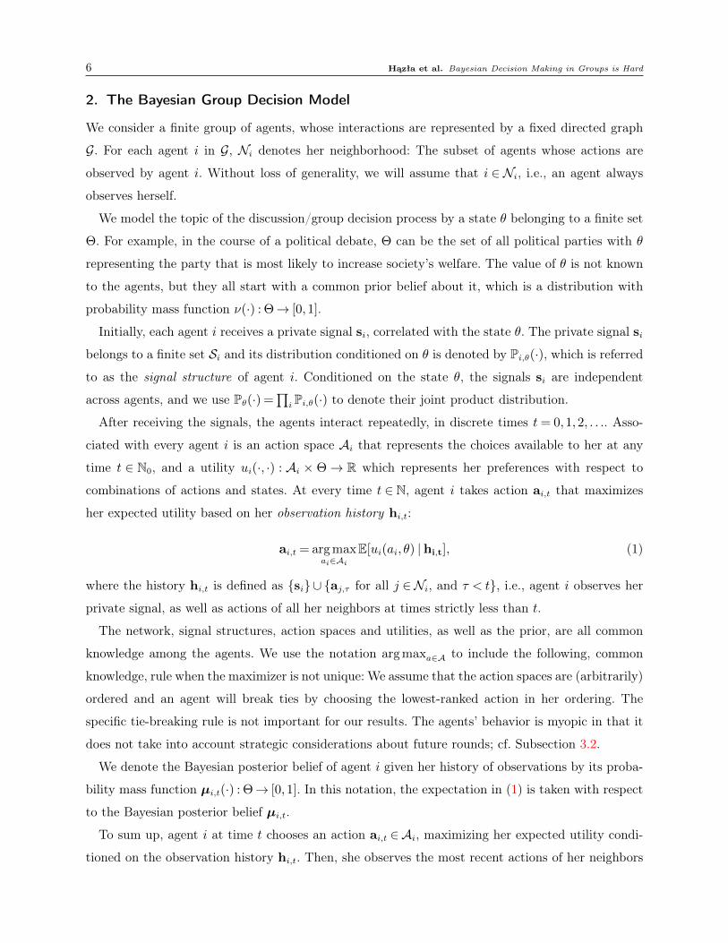
Hązła et al. Bayesian Decision Making in Groups is Hard 7
Figure 1 The Decision Flow Diagram for Two Bayesian Agents
aj,t for all j ∈ Ni, updates her action to ai,t+1 ∈ Ai, and so on. A decision flow diagram for an
example of two interacting agents is provided in Figure 1.
Our main focus in this paper is on the computational and algorithmic aspects of the group decision
process. Specifically, we will be concerned with the following computational problem:
Problem 1 (GROUP-DECISION). At a time t, given the graph structure G, agent i and the
observation history hi,t, determine the Bayesian action ai,t.
2.1. Natural Utility Functions: Binary Actions and Revealed Beliefs
A natural example of a utility function is based on the idea of repeated voting, for example, as an
idealized model of jury deliberations or the papal conclave in the Catholic Church. In this model,
the possible actions correspond to the states of the world, i.e., Ai = Θ and the utilities are given by
ui(a, θ) = 1(a= θ). In other words, the agents receive a unit reward for guessing the state correctly
and zero otherwise. The expected reward of agent i at time t is maximized by choosing the action
that corresponds to the maximum probability in µi,t, i.e. the maximum a posteriori probability
(MAP) estimate. In case of binary world Θ = 0,1 with uniform prior and binary private signals
Si = 0,1 we call this example the binary action model.
In another important example, which we call the revealed belief model, the agents reveal their
complete posteriors, i.e., µi,t. Formally, let Θ := θ1, . . . , θm and let ej ∈Rm be a column vector of
all zeros except for its j-th element which is equal to one. Furthermore, we relax the requirement
that the action spaces Ai are finite sets; instead, for each agent i∈ [n] let Ai be the m-dimensional
probability simplex: Ai = (x1, . . . , xm)T ∈ Rm :∑m
i=1 xi = 1 and xi ≥ 0,∀i. If the utility assigned
to an action a := (a1, . . . , am)T ∈ Ai and a state θj ∈ Θ measures the squared Euclidean distance
between a and ej, then it is optimal for agent i to reveal her belief ai,t = (µi,t(θ1), . . . ,µi,t(θm))T .
We can state a special case of the GROUP-DECISION model in the revealed belief setting:
8 Hązła et al. Bayesian Decision Making in Groups is Hard
Problem 2 (GROUP-DECISION with revealed beliefs). At any time t, given the graph
structure G, agent i and the observation history hi,t, determine the Bayesian posterior belief µi,t.
2.2. Log-Likelihood Ratio and Log-Belief Ratio Notations
Consider a finite state space Θ = θ1, . . . , θm and for all 2≤ k≤m and s∈ Si, let:
λi(s, θk) := log
(Pi,θk(s)
Pi,θ1(s)
), φi,t(θk) := log
(µi,t(θk)
µi,t(θ1)
), γ(θk) := log
(ν(θk)
ν(θ1)
). (2)
We will also write λi(θk) := λi(si, θk). We will call λi the (signal) log-likelihood ratio and φi,t the
log-belief ratio. If we assume that the agents start from uniform prior beliefs and the size of the state
space is m= 2 (as will be the case for the hardness results in Section 3), we can employ a simpler
notation. First, with uniform priors, we have γ(θk) = log (ν(θk)/ν(θ1)) = 0 for all k. Moreover, with
binary state space Θ = 0,1 we only need to keep track of one set of log-belief and log-likelihood
ratios λi := λi(1) = log (Pi,1(si)/Pi,0(si)), and φi,t = φi,t(1) = log (µi,t(1)/µi,t(0)). Henceforth, we
use λi and φi,t as there is no risk of confusion in dropping their arguments.
Note that in the setting with binary state and signals (Si = 0,1), there is a one-to-one corre-
spondence between informative signal structures satisfying Pi,0(1) 6= Pi,1(1), and log-likelihood ratios
satisfying λi(0) · λi(1) < 0. Accordingly, we sometimes use log-likelihood ratios to specify signal
structures.
Example 1 (Belief Exchange in the First Two Rounds). To give some intuition about
our model and illustrate the usefulness of the log-likelihood ratio and log-belief ratio notations, we
explain how the agents in the binary action model can compute their actions at t= 0 and t= 1. We
consider informative binary private signals si ∈ 0,1 with Pi,1(1)> Pi,0(1). We focus on computing
the log-likelihood ratio (φi,t), since ai,t = 1 if, and only if, φi,t > 0.
At time zero, the posterior and log-belief ratio of agent i are determined by her private signal, as
follows:
µi,0(1) =Pi,1(si)
Pi,0(si) +Pi,1(si), φi,0 = log
(Pi,1(si)
Pi,0(si)
).
Therefore, we get ai,0 = si since Pi,1(1) > Pi,0(1). At time one, agent i observes the actions, and
therefore infers the private signals, of her neighbors. Since the private signals are conditionally
independent, the respective log-likelihood ratios add up and we get the following expression (recall
that i∈Ni):
φi,1 =∑j∈Ni
φj,0 =∑j∈Ni
log
(Pj,1(aj,0)
Pj,0(aj,0)
)=∑j∈Ni
λj . (3)
However, the computation becomes significantly more involved at later times. This is because one
needs to account for dependencies and redundancies in agents’ information and the resulting actions.
Hązła et al. Bayesian Decision Making in Groups is Hard 9
(A) (B)
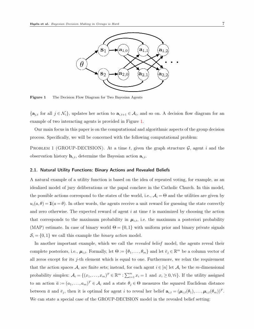
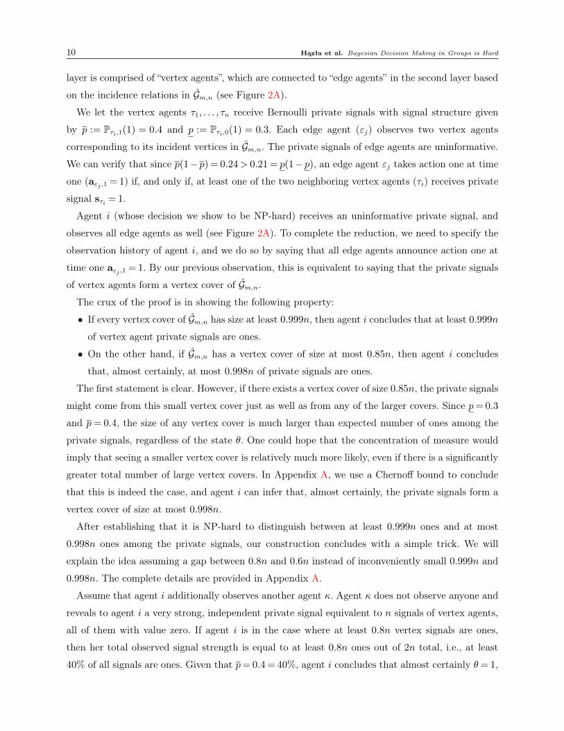
Figure 2 (A) Illustration of the VERTEX-COVER reduction (Theorem 1); every edge εj is connected to its two
vertices, and every vertex is connected to all its incident edges. (B) Illustration of the EXACT-COVER
reduction (Theorem 2); every element εj belongs to exactly three sets and every set τj contains exactly
three elements.
3. Hardness of Bayesian Decisions
Our hardness results use a standard approach from complexity theory; cf., e.g., Arora and Barak
(2009). We establish NP-hardness of computations in both binary action and revealed belief models.
We do so by exhibiting reductions from problems that are known to be NP-hard. As shown below,
two covering problems: vertex cover and set cover, turn out to be convenient starting points for our
reductions. We now present our main hardness results.
Theorem 1 (Binary Action Model). The GROUP-DECISION problem in the binary action
model is NP-hard at t= 2. Furthermore, for a network of n Bayesian agents in the binary action
model, it is NP-hard to distinguish between posterior beliefs µi,2(0) < exp(−Ω(n)) and µi,2(1) <
exp(−Ω(n)).
Proof sketch of Theorem 1. Appendix A contains a detailed proof. Our reduction is from an NP-
hard problem of approximating vertex cover (VERTEX-COVER). A vertex cover on an undirected
graph Gm,n with n vertices and m edges is a subset of vertices (denoted by Σ), such that each
edge touches at least one vertex in Σ. We consider the approximation version of VERTEX-COVER,
where every input graph belongs to one of two cases:
(i) the YES case, where it has at least one small vertex cover (say, smaller than 0.85n),
(ii) the NO case, where all its vertex covers are large (say, larger than 0.999n).
It is NP-hard to distinguish between these two cases.
We show an efficient reduction that maps a graph Gm,n to an instance of GROUP-DECISION in
the binary action model. We encode the structure of Gm,n by a two-layer network, where the first
10 Hązła et al. Bayesian Decision Making in Groups is Hard
layer is comprised of “vertex agents”, which are connected to “edge agents” in the second layer based
on the incidence relations in Gm,n (see Figure 2A).
We let the vertex agents τ1, . . . , τn receive Bernoulli private signals with signal structure given
by p := Pτi,1(1) = 0.4 and p := Pτi,0(1) = 0.3. Each edge agent (εj) observes two vertex agents
corresponding to its incident vertices in Gm,n. The private signals of edge agents are uninformative.
We can verify that since p(1−p) = 0.24> 0.21 = p(1−p), an edge agent εj takes action one at time
one (aεj ,1 = 1) if, and only if, at least one of the two neighboring vertex agents (τi) receives private
signal sτi = 1.
Agent i (whose decision we show to be NP-hard) receives an uninformative private signal, and
observes all edge agents as well (see Figure 2A). To complete the reduction, we need to specify the
observation history of agent i, and we do so by saying that all edge agents announce action one at
time one aεj ,1 = 1. By our previous observation, this is equivalent to saying that the private signals
of vertex agents form a vertex cover of Gm,n.
The crux of the proof is in showing the following property:
• If every vertex cover of Gm,n has size at least 0.999n, then agent i concludes that at least 0.999n
of vertex agent private signals are ones.
• On the other hand, if Gm,n has a vertex cover of size at most 0.85n, then agent i concludes
that, almost certainly, at most 0.998n of private signals are ones.
The first statement is clear. However, if there exists a vertex cover of size 0.85n, the private signals
might come from this small vertex cover just as well as from any of the larger covers. Since p= 0.3
and p= 0.4, the size of any vertex cover is much larger than expected number of ones among the
private signals, regardless of the state θ. One could hope that the concentration of measure would
imply that seeing a smaller vertex cover is relatively much more likely, even if there is a significantly
greater total number of large vertex covers. In Appendix A, we use a Chernoff bound to conclude
that this is indeed the case, and agent i can infer that, almost certainly, the private signals form a
vertex cover of size at most 0.998n.
After establishing that it is NP-hard to distinguish between at least 0.999n ones and at most
0.998n ones among the private signals, our construction concludes with a simple trick. We will
explain the idea assuming a gap between 0.8n and 0.6n instead of inconveniently small 0.999n and
0.998n. The complete details are provided in Appendix A.
Assume that agent i additionally observes another agent κ. Agent κ does not observe anyone and
reveals to agent i a very strong, independent private signal equivalent to n signals of vertex agents,
all of them with value zero. If agent i is in the case where at least 0.8n vertex signals are ones,
then her total observed signal strength is equal to at least 0.8n ones out of 2n total, i.e., at least
40% of all signals are ones. Given that p= 0.4 = 40%, agent i concludes that almost certainly θ= 1,
Hązła et al. Bayesian Decision Making in Groups is Hard 11
i.e., µi,2(0) ≈ 0. On the other hand, in case where (almost certainly) at most 0.6n vertex signals
are ones, total signal strength is at most 0.6n out of 2n, i.e., 30% of possible signals and, recalling
p= 0.3 = 30%, agent i concludes that µi,2(1)≈ 0.1
Remark 1. A priori one might suspect that the difficulty of distinguishing between ai,2 = 0 and
ai,2 = 1 arises only if the belief of agent i is very close to the threshold µi,2 ≈ 1/2. However, in our
reduction the opposite is true: For a computationally bounded agent, it is hopeless to distinguish
between worlds where θ= 0 with high probability (w.h.p.), and θ= 1 w.h.p. This can be thought of
as a strong hardness of approximation result.
We also have a matching result for the revealed belief model:
Theorem 2 (Approximating Beliefs). The GROUP-DECISION problem is NP-hard in the
revealed belief model with uniform priors, binary states Θ = 0,1, and binary private signals si ∈0,1. In particular, for a network of n Bayesian agents at t= 2, it is NP-hard to distinguish between
beliefs µi,2(0)≤ exp(−Ω(n)) and µi,2(1)≤ exp(−Ω(n)).
Proof sketch for Theorem 2. Appendix B contains a detailed proof. Our reduction is from a
variant of an NP-complete problem EXACT-COVER. Let n be a multiple of three and consider
a set of n elements En = ε1, . . . , εn and a family of n subsets of En denoted by Tn = τ1, . . . , τn,τj ⊂ En for all j ∈ [n]. EXACT-COVER is the problem of deciding if there exists a collection T ⊆ Tnthat exactly covers En, that is, each element εi belongs to exactly one set in T . We use a restriction
of EXACT-COVER where each set has size three and each element appears in exactly three sets;
hence, if the exact cover exists, then it consist of n/3 sets.
We use a two-layer network to encode the inclusion relations between the elements En and subsets
Tn. There are n agents τ1, . . . , τn in the first layer to encode the subsets and n agents ε1, . . . , εn
in the second layer to encode the elements. Each “element agent” observes three “subset agents”
corresponding to subsets to which the element belongs (see Figure 2B). Agent i (whose decision we
show to be NP-hard) observes the reported beliefs of all element agents. There is also one auxiliary
agent κ that is observed by all element agents.
The private signals of agent i and the element agents are non-informative. The subset agents
observe i.i.d. binary signals and the auxiliary agent κ observes another independent binary signal,
but with a different distribution. We set up the signal structures and the beliefs transmitted by the
element agents to agent i such that there are two possible outcomes: Either sκ = 0 and all subset
agents received positive signals sτi = 1; or, sκ = 1 and the private signals of subset agents form an
exact cover of the elements. Of course, the second alternative is possible only if an exact cover exists.
The first alternative implies that all subset agents received ones as private signals, and therefore
θ = 1 with high probability. In case of the second alternative, we show that almost certainly only

12 Hązła et al. Bayesian Decision Making in Groups is Hard
one-third of subset agents received ones, and therefore θ = 0 with high probability. Therefore, if
there is no exact cover, agent i should compute µi,2(0)≈ 0 and otherwise µi,2(1)≈ 0.
We conclude this section by discussing some aspects and limitations of our proof. We also examine
the economic assumptions behind our results and discuss what happens when these assumptions
are relaxed.
3.1. Worst-Case and Average-Case Reductions
Our reductions are worst-case, both with respect to networks and signal profiles. That is, we show
hardness only for a specific class of networks, and for signal profiles in those networks that arise with
exponentially small probability. We cannot exclude existence of an efficient algorithm that computes
Bayesian beliefs for all network structures, with high probability over signal profiles. Notwithstand-
ing, any such purported algorithm must have a good reason to fail on our hard instances.
This reflects a general phenomenon in computational complexity, where average-case hardness,
even when suspected to hold, seems to be significantly more difficult to rigorously demonstrate (see
Bogdanov et al. (2006) for one survey). We leave as a fascinating open problem if our results can be
improved, for example for worst-case networks and average-case signal profiles. One thing to note
in this regard is that our reductions encode the witnesses to NP problems (vertex and set covers)
as signal profiles. That necessarily means that for hard positive instances (e.g., graphs with a small
vertex cover) relevant signal profiles will arise only with tiny probability: Otherwise these instances
would be easy to solve by sampling a potential witness at random. Significant new ideas might be
needed to overcome this problem.
On the positive side, the worst-case nature of our hard instances makes it potentially easier to
embed them in more general or modified settings. We discuss several concrete cases below.
3.2. Forward-looking Agents
Our results are restricted to myopic agents. In the general framework of forward-looking utility
maximizers with discount factor δ, myopic agents are obtained as a special case by completely
discounting the future pay-offs (δ→ 0).
The computational difficulties for strategic agents seem to be at least as large as for myopic
agents, but we do not offer any formal results. Due to the multiplicity of equilibria suggested by
the folk theorem (Fudenberg and Maskin 1986) — see also examples in Rosenberg et al. (2009) and
Mossel et al. (2015) — it is unclear to us how to make the computational problem well-posed. On
the other hand, since in the limit t→∞ the agents in any equilibrium act myopically (Rosenberg
et al. 2009), it seems plausible to expect that their computations will be similarly hard as in our
analysis.

Hązła et al. Bayesian Decision Making in Groups is Hard 13
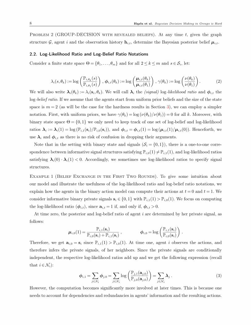
(A) (B) (C) (D)
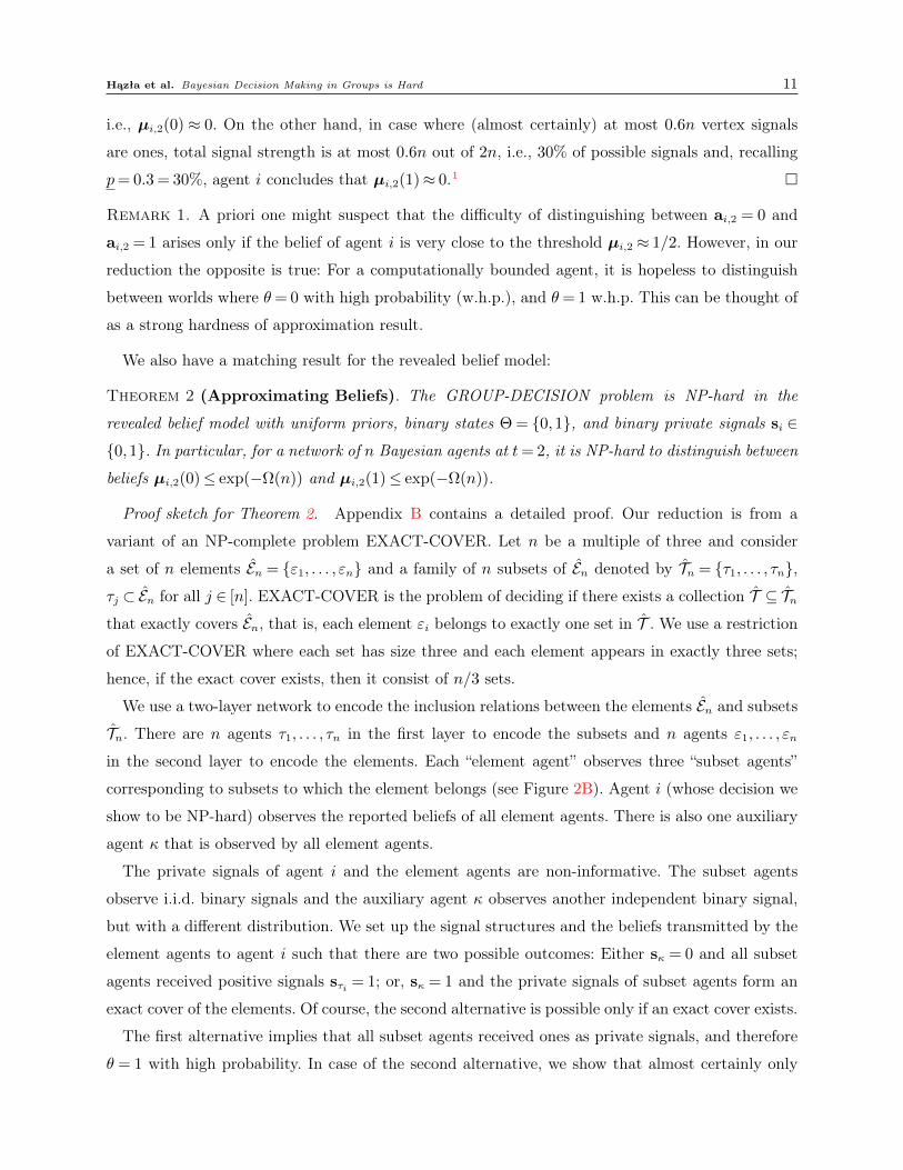
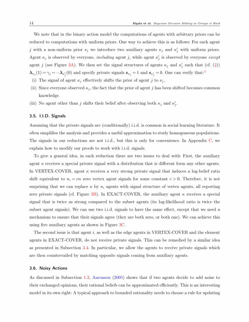
Figure 3 (A) We can cancel out the effect of a distinct, non-uniform prior in an agent j by adding two auxiliary
agents (κj and κ′j), and have agent j observe only one of them. Both added agents will be observed by
every other agent. (B) We can replace the auxiliary agent κ in the VERTEX-COVER reduction by ni
agents ι1, . . ., ιni with zero signals drawn from the same i.i.d distribution as the vertex agents. (C) We
can replace the auxiliary agent κ in the EXACT-COVER reduction by five agents κ1, . . ., κ5 with i.i.d.
signals and set up their received signals and the observation structure such that the signals of κ1 and
κ3 necessarily agree. (D) We can modify the VERTEX-COVER reduction to work with noisy binary
actions. Here each pair of vertex agents (ε(1) and ε(2)) are observed by a collection of edge agents ε(1),
. . . , ε(k) who all report the same noisy actions a′ε(1),1 = . . .= a′ε(k),1 = 1.
3.3. Directed Links
In both our reductions, we use directed acyclic graphs. This is arguably a simpler case from an
inference viewpoint, since in networks containing cycles (including those with bidirectional links) an
agent needs to take into account her own, possibly indirect, influence on her neighbors. Therefore,
our hardness results hold true, in spite of the (simpler) acyclic structure of our hard examples.
In effect, our hardness results are applicable to undirected (bidirectional) networks without loss
of generality. The reason is that replacing directed links with bidirectional ones does not affect
any relevant inferences in our reductions. In particular, our results apply to networks that exhibit
agreement and learning, cf. Mossel et al. (2014). It is worth noting that since our results are achieved
in a basic model with binary state and private signals, they can be easily embedded in richer settings,
e.g., with signal structures given by continuous distributions.
3.4. Common Priors
The common prior assumption simplifies the belief calculations in our hard examples, but it does
not play a critical role otherwise. In fact, we can argue that similar to the directed links, imposition
of common priors on the agents simplifies their inference tasks. This is consistent with the fact that
common priors are crucial for reaching agreement (Aumann 1976).
14 Hązła et al. Bayesian Decision Making in Groups is Hard
We note that in the binary action model the computations of agents with arbitrary priors can be
reduced to computations with uniform priors. One way to achieve this is as follows: For each agent
j with a non-uniform prior νj we introduce two auxiliary agents κj and κ′j with uniform priors.
Agent κj is observed by everyone, including agent j, while agent κ′j is observed by everyone except
agent j (see Figure 3A). We then set the signal structures of agents κj and κ′j such that (cf. (2))
λκj (1) = γj =−λκ′j (0) and specify private signals sκj = 1 and sκ′j = 0. One can verify that:2
(i) The signal of agent κj effectively shifts the prior of agent j to νj.
(ii) Since everyone observed κj, the fact that the prior of agent j has been shifted becomes common
knowledge.
(iii) No agent other than j shifts their belief after observing both κj and κ′j.
3.5. I.I.D. Signals
Assuming that the private signals are (conditionally) i.i.d. is common in social learning literature. It
often simplifies the analysis and provides a useful approximation to study homogeneous populations.
The signals in our reductions are not i.i.d., but this is only for convenience. In Appendix C, we
explain how to modify our proofs to work with i.i.d. signals.
To give a general idea, in each reduction there are two issues to deal with: First, the auxiliary
agent κ receives a special private signal with a distribution that is different form any other agents.
In VERTEX-COVER, agent κ receives a very strong private signal that induces a log-belief ratio
shift equivalent to ni = cn zero vertex agent signals for some constant c > 0. Therefore, it is not
surprising that we can replace κ by ni agents with signal structure of vertex agents, all reporting
zero private signals (cf. Figure 3B). In EXACT-COVER, the auxiliary agent κ receives a special
signal that is twice as strong compared to the subset agents (its log-likelihood ratio is twice the
subset agent signals). We can use two i.i.d. signals to have the same effect, except that we need a
mechanism to ensure that their signals agree (they are both zero, or both one). We can achieve this
using five auxiliary agents as shown in Figure 3C.
The second issue is that agent i, as well as the edge agents in VERTEX-COVER and the element
agents in EXACT-COVER, do not receive private signals. This can be remedied by a similar idea
as presented in Subsection 3.4. In particular, we allow the agents to receive private signals which
are then countervailed by matching opposite signals coming from auxiliary agents.
3.6. Noisy Actions
As discussed in Subsection 1.2, Aaronson (2005) shows that if two agents decide to add noise to
their exchanged opinions, their rational beliefs can be approximated efficiently. This is an interesting
model in its own right: A typical approach to bounded rationality needs to choose a rule for updating
Hązła et al. Bayesian Decision Making in Groups is Hard 15
beliefs, and any such choice is, to an extent, arbitrary. If, instead, it could be shown that “noisy”
Bayesian updates are efficient, it would provide for an interesting alternative.
Notwithstanding, we show that adding noise does not change our hardness results for network
models. For concreteness, we focus on a particular modification of the binary action model. However,
we believe our ideas should work with most other natural variants. More precisely, we consider the
binary action model with an additional parameter 0< δ < 1/2. All the rules are the same except that
every time an agent broadcasts her opinion to the world, a glitch (bit flip) occurs with probability
δ.
In other words, every time agent i computes an action ai,t = 1(µi,t > 1/2), its announced value
(a′i,t) is flipped to 1 − ai,t, independently with probability δ. We assume that all neighbors of i
observe the same action (as opposed to flipping with probability δ independently for each neighbor).
Since the networks that we consider are acyclical, it does not matter if the agents observe their
own actions, i.e., if they learn that their actions were flipped. As before, all these rules are common
knowledge and the agents estimate their beliefs (µi,t) using the Bayes rule.
In Appendix D we show that estimating beliefs in this model is still NP-hard. The main idea is
that an agent in the noiseless binary action model can be replaced with multiple copies of noisy
agents broadcasting the same action in such a way that the probability of the transmission error is
negligible compared to the other probabilities that determine the computed beliefs (see Figure 3D).
4. Algorithms for Bayesian Choice
Refinement of information partitions with increasing observations is a key feature of rational learning
problems and it is fundamental to major classical results that establish agreement (Geanakoplos and
Polemarchakis (1982)) or learning (Blackwell and Dubins (1962), Lehrer and Smorodinsky (1996))
among rational agents.
In the group decision setting, the list of possible signal profiles is regarded as the information set
representing the current understanding of the agent about her environment, and the way additional
observations are informative is by trimming the current information set and reducing the ambiguity
in the set of initial signals that have caused the agent’s history of past observations. Thereby, one
can conceive a natural method of computing agents’ actions based on elimination of impossible
signals. By successively eliminating signals that are inconsistent with the new observations, we
refine the partitions of the space of private signals, and at the same time, we keep track of the
current information set that is consistent with the observations. As such, we refer to this approach
as “Elimination of Impossible Signals” or EIS. We begin by presenting a recursive version (REIS),
and study its iterative implementations (IEIS) afterwards.
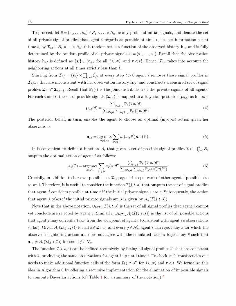
16 Hązła et al. Bayesian Decision Making in Groups is Hard
To proceed, let s= (s1, . . . , sn)∈ S1× . . .×Sn be any profile of initial signals, and denote the set
of all private signal profiles that agent i regards as possible at time t, i.e. her information set at
time t, by I i,t ⊂S1× . . .×Sn; this random set is a function of the observed history hi,t and is fully
determined by the random profile of all private signals s := (s1, . . . , sn). Recall that the observation
history hi,t is defined as si ∪ aj,τ for all j ∈ Ni, and τ < t. Hence, I i,t takes into account the
neighboring actions at all times strictly less than t.
Starting from I i,0 = si ×∏j 6=i Sj, at every step t > 0 agent i removes those signal profiles in
I i,t−1 that are inconsistent with her observation history hi,t, and constructs a censured set of signal
profiles I i,t ⊂ I i,t−1. Recall that Pθ(·) is the joint distribution of the private signals of all agents.
For each i and t, the set of possible signals (I i,t) is mapped to a Bayesian posterior (µi,t) as follows:
µi,t(θ) =
∑s∈Ii,t
Pθ(s)ν(θ)∑θ′∈Θ
∑s∈Ii,t
Pθ′(s)ν(θ′). (4)
The posterior belief, in turn, enables the agent to choose an optimal (myopic) action given her
observations:
ai,t = arg maxai∈Ai
∑θ′∈Θ
ui(ai, θ′)µi,t(θ
′). (5)
It is convenient to define a function Ai that given a set of possible signal profiles I ⊂∏n
j=1 Sjoutputs the optimal action of agent i as follows:
Ai(I) = arg maxa∈Ai
∑θ′∈Θ
ui(a, θ′)
∑s′∈I Pθ′(s
′)ν(θ′)∑θ′′∈Θ
∑s′∈I Pθ′′(s
′)ν(θ′′). (6)
Crucially, in addition to her own possible set I i,t, agent i keeps track of other agents’ possible sets
as well. Therefore, it is useful to consider the function I(j, t, s) that outputs the set of signal profiles
that agent j considers possible at time t if the initial private signals are s. Subsequently, the action
that agent j takes if the initial private signals are s is given by Aj(I(j, t, s)).
Note that in the above notation, ∪s∈Ii,tI(j, t, s) is the set of all signal profiles that agent i cannot
yet conclude are rejected by agent j. Similarly, ∪s∈Ii,tAj(I(j, t, s)) is the list of all possible actions
that agent j may currently take, from the viewpoint of agent i (consistent with agent i’s observations
so far). Given Aj(I(j, t, s)) for all s∈ I i,t−1 and every j ∈Ni, agent i can reject any s for which the
observed neighboring action aj,t does not agree with the simulated action: Reject any s such that
aj,t 6=Aj(I(j, t, s)) for some j ∈Ni.The function I(i, t, s) can be defined recursively by listing all signal profiles s′ that are consistent
with s, producing the same observations for agent i up until time t. To check such consistencies one
needs to make additional function calls of the form I(j, τ, s′) for j ∈Ni and τ < t. We formalize this
idea in Algorithm 0 by offering a recursive implementation for the elimination of impossible signals
to compute Bayesian actions (cf. Table 1 for a summary of the notation).3

Hązła et al. Bayesian Decision Making in Groups is Hard 17
Table 1 Notation for Bayesian group decision computations (Elimination of Impossible Signals)
s=(s1, s2, . . . , sn)
a profile of initial private signals.
I i,t the set of all signal profiles that are deemed possible by agent i, givenher observations up until time t.
I(j, t, s) the set of all signal profiles that are deemed possible by agent j attime t, if the initial signals of all agents are prescribed according to s.
Aj(I(j, t, s)) the computed action of agent j at time t, if the initial signals of allagents are prescribed according to s.
Algorithm 0: RECURSIVE-EIS (i, t)Input: Graph G, set of possible signal profiles I i,t, and neighboring actions aj,t, j ∈NiOutput: Bayesian action ai,t+1
1. Initialize I i,t+1 = I i,t.2. For all s∈ I i,t+1, do:
• For all j ∈Ni, if aj,t 6=Aj(I(j, t, s)), then set I i,t+1 = I i,t+1 \ s.3. ai,t+1 =Ai(I i,t+1).
Function I(i, t, s) :• If t= 0, then set I = si×
∏j 6=i Sj
• else if t > 0:1. Initialize I =∅.2. For all s′ ∈ S1× . . .×Sn, do:
—If Consistent(i, t, s, s′), then set I = I ∪s′.return IFunction Consistent(i, t, s, s′):1. Initialize is_consistent = True.2. For all τ < t and j ∈Ni, do:
• If Aj(I(j, τ, s)) 6=Aj(I(j, τ, s′)), then is_consistent = False.return is_consistent
In Subsection 4.1, we describe an iterative implementation of elimination of impossible signals
(IEIS). The IEIS calculations scale exponentially with the network size; this is true, in general,
with the exception of some densely connected networks where agents have direct access to all
the observations of their neighbors. We expand on this special case (called transitive networks) in
Subsection 4.2. Finally, in Subsection 4.3 we discuss the revealed beliefs case and identify additional
network structures for which Bayesian calculations simplify, allowing for efficient Bayesian belief
exchange.
4.1. Iterative Elimination of Impossible Signals (IEIS)
To proceed, we denote N τi as the τ -th order neighborhood of agent i comprising entirely of those
agents who are at distance τ from agent i; in particular, N 1i = Ni, and we use the convention
18 Hązła et al. Bayesian Decision Making in Groups is Hard
N 0i = i. We further denote N t
i :=∪tτ=0N τi as the set of all agents who are within distance t of or
closer to agent i; we sometimes refer to N ti as her ego-net of radius t.
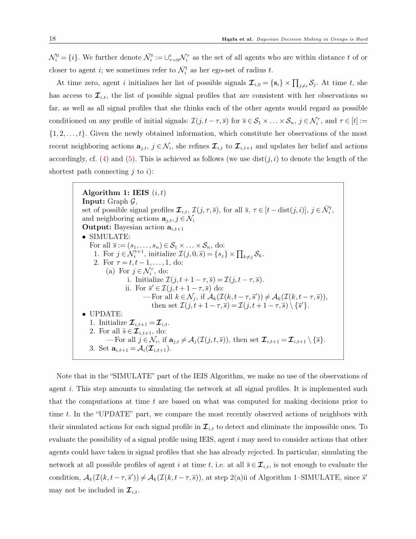
At time zero, agent i initializes her list of possible signals I i,0 = si ×∏j 6=i Sj. At time t, she
has access to I i,t, the list of possible signal profiles that are consistent with her observations so
far, as well as all signal profiles that she thinks each of the other agents would regard as possible
conditioned on any profile of initial signals: I(j, t− τ, s) for s∈ S1× . . .×Sn, j ∈N τi , and τ ∈ [t] :=
1,2, . . . , t. Given the newly obtained information, which constitute her observations of the most
recent neighboring actions aj,t, j ∈Ni, she refines I i,t to I i,t+1 and updates her belief and actions
accordingly, cf. (4) and (5). This is achieved as follows (we use dist(j, i) to denote the length of the
shortest path connecting j to i):
Algorithm 1: IEIS (i, t)Input: Graph G,set of possible signal profiles I i,t, I(j, τ, s), for all s, τ ∈ [t− dist(j, i)], j ∈ N t
i ,and neighboring actions aj,t, j ∈NiOutput: Bayesian action ai,t+1
• SIMULATE:For all s := (s1, . . . , sn)∈ S1× . . .×Sn, do:1. For j ∈N t+1
i , initialize I(j,0, s) = sj×∏k 6=j Sk.
2. For τ = t, t− 1, . . . ,1, do:(a) For j ∈N τ
i , do:i. Initialize I(j, t+ 1− τ, s) = I(j, t− τ, s).ii. For s′ ∈ I(j, t+ 1− τ, s) do:
—For all k ∈Nj, if Ak(I(k, t− τ, s′)) 6=Ak(I(k, t− τ, s)),then set I(j, t+ 1− τ, s) = I(j, t+ 1− τ, s) \ s′.
• UPDATE:1. Initialize I i,t+1 = I i,t.2. For all s∈ I i,t+1, do:
—For all j ∈Ni, if aj,t 6=Aj(I(j, t, s)), then set I i,t+1 = I i,t+1 \ s.3. Set ai,t+1 =Ai(I i,t+1).
Note that in the “SIMULATE” part of the IEIS Algorithm, we make no use of the observations of
agent i. This step amounts to simulating the network at all signal profiles. It is implemented such
that the computations at time t are based on what was computed for making decisions prior to
time t. In the “UPDATE” part, we compare the most recently observed actions of neighbors with
their simulated actions for each signal profile in I i,t to detect and eliminate the impossible ones. To
evaluate the possibility of a signal profile using IEIS, agent i may need to consider actions that other
agents could have taken in signal profiles that she has already rejected. In particular, simulating the
network at all possible profiles of agent i at time t, i.e. at all s∈ I i,t, is not enough to evaluate the
condition, Ak(I(k, t− τ, s′)) 6=Ak(I(k, t− τ, s)), at step 2(a)ii of Algorithm 1–SIMULATE, since s′
may not be included in I i,t.

Hązła et al. Bayesian Decision Making in Groups is Hard 19
Table 2 Notation for Computations in Transitive Networks
Si,t
the list of all private signals that are deemed possible for agent i at time t,by an agent who has observed her actions in a transitive network structureup until time t.
I i,t(si) = si×∏j∈Ni
Sj,t
the list of neighboring signal profiles that are deemed possible by agent i,given her observations of their actions up until time t conditioned on ownprivate signal being si.
In Appendix E we describe the complexity of the computations that the agent should undertake
using IEIS at any time t in order to calculate her posterior probability µi,t+1 and Bayesian decision
ai,t+1 given all her observations up to time t. Subsequently, we prove that:
Theorem 3 (Complexity of IEIS). Consider a network of size n with m states, and let M
and A denote the maximum cardinality of the signal and action spaces (m :=card(Θ), M =
maxk∈[n]card(Sk), and A = maxk∈[n]card(Ak)). The IEIS algorithm has O(n2M 2n−1mA) running
time, which given the private signal of agent i and the previous actions of her neighbors aj,τ : j ∈
Ni, τ < t in any network structure, outputs ai,t, the Bayesian action of agent i at a fixed time t.
4.2. IEIS over Transitive Structures
We now shift focus to the special case of transitive networks, defined below.
Definition 1 (Transitive Networks). We call a network structure transitive if the directed
neighborhood relationship between its nodes satisfies the reflexive and transitive properties. In
particular, the transitive property implies that anyone whose actions indirectly influence the obser-
vations of agent i is also directly observed by her, i.e. any neighbor of a neighbor of agent i is a
neighbor of agent i as well.
In such structures, any agent whose actions indirectly influence the observations of agent i is
also directly observed by her. This special structure of transitive networks mitigates the issue of
hidden observations, and as a result, Bayesian inference in a transitive structure is significantly less
complex.
After initializing Sj,0 = Sj and I i,0 = si ×∏j∈Ni
Sj,0, agent i needs only to keep track of
Sj,t ⊆ Sj for all j ∈ Ni (cf. Table 2). This is because, in transitive structures, the list of possible
signal profiles decomposes: I i,t = si×∏j∈Ni
Sj,t. Updating in transitive structures is achieved by
incorporating aj,t for each j ∈Ni individually, and transforming the respective Sj,t into Sj,t+1. This
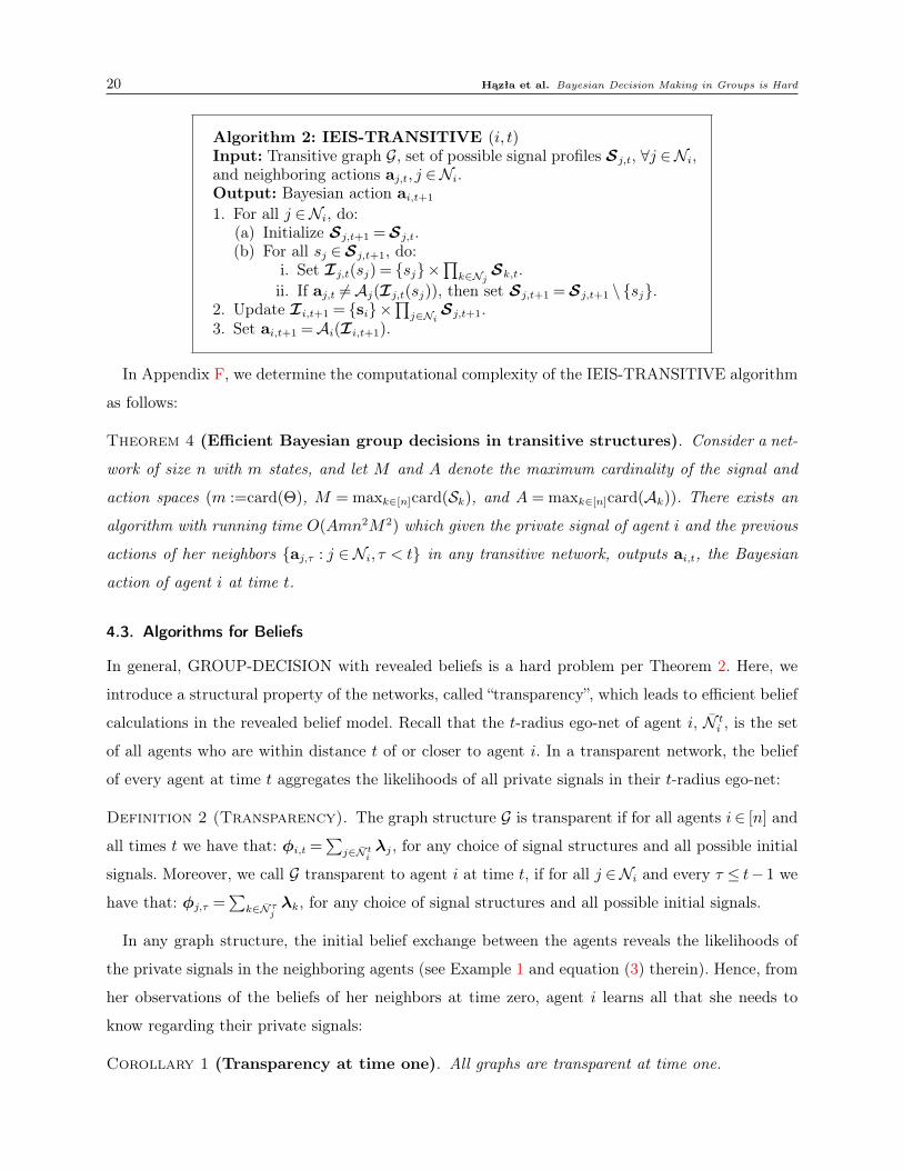
updating procedure is formalized in Algorithm 2.
20 Hązła et al. Bayesian Decision Making in Groups is Hard
Algorithm 2: IEIS-TRANSITIVE (i, t)Input: Transitive graph G, set of possible signal profiles Sj,t, ∀j ∈Ni,and neighboring actions aj,t, j ∈Ni.Output: Bayesian action ai,t+1
1. For all j ∈Ni, do:(a) Initialize Sj,t+1 =Sj,t.(b) For all sj ∈Sj,t+1, do:
i. Set Ij,t(sj) = sj×∏k∈Nj
Sk,t.ii. If aj,t 6=Aj(Ij,t(sj)), then set Sj,t+1 =Sj,t+1 \ sj.
2. Update I i,t+1 = si×∏j∈Ni
Sj,t+1.3. Set ai,t+1 =Ai(I i,t+1).
In Appendix F, we determine the computational complexity of the IEIS-TRANSITIVE algorithm
as follows:
Theorem 4 (Efficient Bayesian group decisions in transitive structures). Consider a net-
work of size n with m states, and let M and A denote the maximum cardinality of the signal and
action spaces (m :=card(Θ), M = maxk∈[n]card(Sk), and A = maxk∈[n]card(Ak)). There exists an
algorithm with running time O(Amn2M 2) which given the private signal of agent i and the previous
actions of her neighbors aj,τ : j ∈ Ni, τ < t in any transitive network, outputs ai,t, the Bayesian
action of agent i at time t.
4.3. Algorithms for Beliefs
In general, GROUP-DECISION with revealed beliefs is a hard problem per Theorem 2. Here, we
introduce a structural property of the networks, called “transparency”, which leads to efficient belief
calculations in the revealed belief model. Recall that the t-radius ego-net of agent i, N ti , is the set
of all agents who are within distance t of or closer to agent i. In a transparent network, the belief
of every agent at time t aggregates the likelihoods of all private signals in their t-radius ego-net:
Definition 2 (Transparency). The graph structure G is transparent if for all agents i∈ [n] and
all times t we have that: φi,t =∑
j∈N tiλj, for any choice of signal structures and all possible initial
signals. Moreover, we call G transparent to agent i at time t, if for all j ∈Ni and every τ ≤ t− 1 we
have that: φj,τ =∑
k∈N τjλk, for any choice of signal structures and all possible initial signals.
In any graph structure, the initial belief exchange between the agents reveals the likelihoods of
the private signals in the neighboring agents (see Example 1 and equation (3) therein). Hence, from
her observations of the beliefs of her neighbors at time zero, agent i learns all that she needs to
know regarding their private signals:
Corollary 1 (Transparency at time one). All graphs are transparent at time one.
Hązła et al. Bayesian Decision Making in Groups is Hard 21
However, the future neighboring beliefs (at time two and beyond) are “less transparent” when it
comes to reflecting the neighbors’ knowledge of other private signals that are received throughout
the network. In particular, the time one beliefs of the neighbors φj,1, j ∈ Ni are given by φj,1 =∑k∈N1
jλk; hence, from observing the time one belief of a neighbor, agent i would only get to know∑
k∈Njλk, rather than the individual values of λk for each k ∈Nj.4
Remark 2 (Transparency, statistical efficiency, and impartial inference). Such
agents j whose beliefs satisfy the equation in Definition 2 at some time τ are said to hold a
transparent or efficient belief; the latter signifies the fact that such a belief coincides with the
Bayesian posterior if agent j were given direct access to the private signals of every agent in N τj .
This is indeed the best possible (or statistically efficient) belief that agent j can hope to form
given the information available to her at time τ . The same connection to the statistically efficient
beliefs arise in the work of Eyster and Rabin (2014) who formulate the closely related concept of
“impartial inference” in a model of sequential decisions by different players in successive rounds;
accordingly, impartial inference ensures that the full informational content of all signals that
influence a player’s beliefs can be extracted and players can fully (rather than partially) infer their
predecessors’ signals. In other words, under impartial inference, players’ immediate predecessors
provide “sufficient statistics” for earlier movers that are indirectly observed (Eyster and Rabin 2014,
Section 3). Last but not least, it is worth noting that statistical efficiency or impartial inference
are properties of the posterior beliefs, and as such the signal structures may be designed so that
statistical efficiency or impartial inference hold true for a particular problem setting; on the other
hand, transparency is a structural property of the network and would hold true for any choice of
signal structures and all possible initial signals.
Our next example helps clarify the concept of transparency as a structural graph property, and
its relation to Bayesian belief computations.
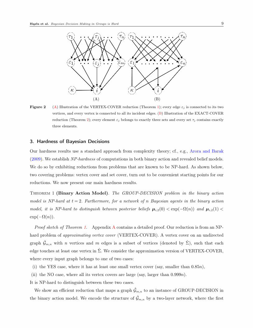
(A) (B) (C) (D)
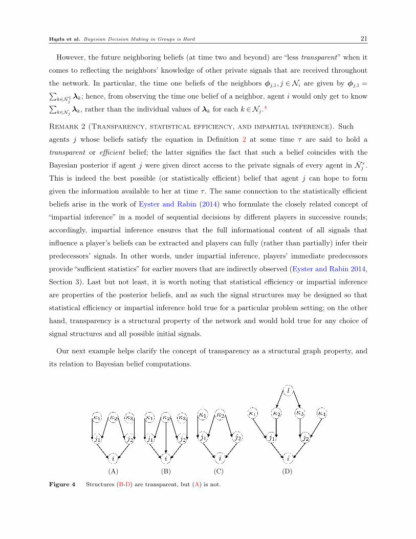
Figure 4 Structures (B-D) are transparent, but (A) is not.
22 Hązła et al. Bayesian Decision Making in Groups is Hard
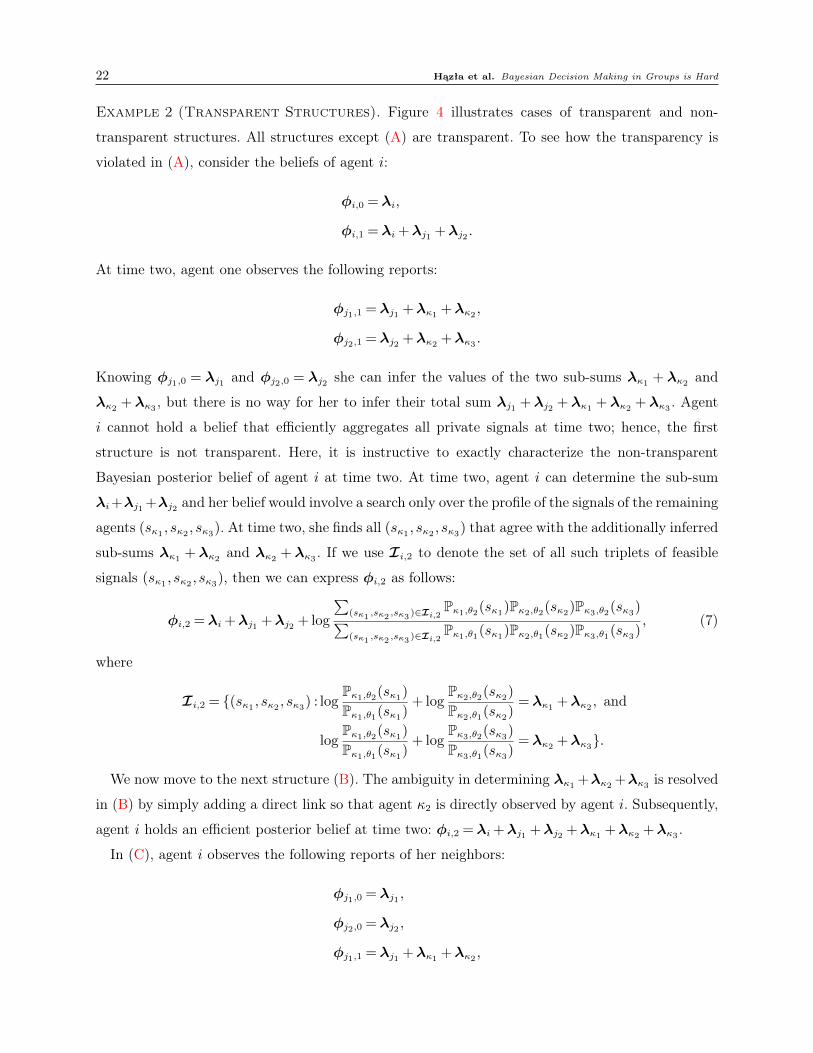
Example 2 (Transparent Structures). Figure 4 illustrates cases of transparent and non-
transparent structures. All structures except (A) are transparent. To see how the transparency is
violated in (A), consider the beliefs of agent i:
φi,0 =λi,
φi,1 =λi +λj1 +λj2 .
At time two, agent one observes the following reports:
φj1,1 =λj1 +λκ1 +λκ2 ,
φj2,1 =λj2 +λκ2 +λκ3 .
Knowing φj1,0 = λj1 and φj2,0 = λj2 she can infer the values of the two sub-sums λκ1 + λκ2 and
λκ2 +λκ3 , but there is no way for her to infer their total sum λj1 +λj2 +λκ1 +λκ2 +λκ3 . Agent
i cannot hold a belief that efficiently aggregates all private signals at time two; hence, the first
structure is not transparent. Here, it is instructive to exactly characterize the non-transparent
Bayesian posterior belief of agent i at time two. At time two, agent i can determine the sub-sum
λi+λj1 +λj2 and her belief would involve a search only over the profile of the signals of the remaining
agents (sκ1 , sκ2 , sκ3). At time two, she finds all (sκ1 , sκ2 , sκ3) that agree with the additionally inferred
sub-sums λκ1 + λκ2 and λκ2 + λκ3 . If we use I i,2 to denote the set of all such triplets of feasible
signals (sκ1 , sκ2 , sκ3), then we can express φi,2 as follows:
φi,2 =λi +λj1 +λj2 + log
∑(sκ1 ,sκ2 ,sκ3 )∈Ii,2
Pκ1,θ2(sκ1)Pκ2,θ2(sκ2)Pκ3,θ2(sκ3)∑(sκ1 ,sκ2 ,sκ3 )∈Ii,2
Pκ1,θ1(sκ1)Pκ2,θ1(sκ2)Pκ3,θ1(sκ3), (7)
where
I i,2 = (sκ1 , sκ2 , sκ3) : logPκ1,θ2(sκ1)
Pκ1,θ1(sκ1)+ log
Pκ2,θ2(sκ2)
Pκ2,θ1(sκ2)=λκ1 +λκ2 , and
logPκ1,θ2(sκ1)
Pκ1,θ1(sκ1)+ log
Pκ3,θ2(sκ3)
Pκ3,θ1(sκ3)=λκ2 +λκ3.
We now move to the next structure (B). The ambiguity in determining λκ1 +λκ2 +λκ3 is resolved
in (B) by simply adding a direct link so that agent κ2 is directly observed by agent i. Subsequently,
agent i holds an efficient posterior belief at time two: φi,2 =λi +λj1 +λj2 +λκ1 +λκ2 +λκ3 .
In (C), agent i observes the following reports of her neighbors:
φj1,0 =λj1 ,
φj2,0 =λj2 ,
φj1,1 =λj1 +λκ1 +λκ2 ,
Hązła et al. Bayesian Decision Making in Groups is Hard 23
and can use these observations at time two, to solve for the sum of log-likelihood ratios of private
signals of everybody:
φi,2 =λi +φj1,1 +φj2,0
=λi +λj1 +λj2 +λκ1 +λκ2
Structure (D) is also transparent. At time two, agent i observes φj1,1 = λj1 + λκ1 + λκ2 and
φj2,1 =λj2 +λκ3 +λκ4 , in addition to her own private signal λi. Her belief at time two is given by:
φi,2 =λi +φj1,1 +φj2,1
=λi +λj1 +λj2 +λκ1 +λκ2 +λκ3 +λκ4 .
A time three, agent i adds φj1,2 = φj1,2 + λl = λj1 + λκ1 + λκ2 + λl to her observations and her
belief at time three is give by:
φi,3 =λi +φj1,1 +φj2,1 + (φj1,2−φj1,1)
=λi +λj1 +λj2 +λκ1 +λκ2 +λκ3 +λκ4 +λl.
This example illustrates a case where an agent learns the sum of log-likelihood ratios of signals of
agents in her higher-order neighborhoods even though she cannot determine each log-likelihood ratio
individually. In structure (D), agent i learns λi,λj1 ,λj2 ,λκ1 +λκ2 ,λκ3 +λκ4 ,λl, and in particular,
she can determine the total sum of log-likelihood ratios of all of the signals in her extended neigh-
borhood, but she never learns the values of the individual log-likelihood ratios λκ1 ,λκ2 ,λκ3 ,λκ4.
The following is a sufficient graphical condition for agent i to hold an efficient (transparent) belief
at time t: there are no agents k ∈ N ti that has multiple paths to agent i, unless it is among her
neighbors (agent k is directly observed by agent i).
Proposition 1 (Graphical Condition for Transparency). Agent i will hold a transparent
(efficient) Bayesian posterior belief at time t if for any k ∈ N ti \Ni there is a unique path from k to
i.
The graphical condition that is proposed above is only sufficient. For example, structures (C)
and (D) in Example 2 violate this condition, despite both being transparent. We present the proof
of Proposition 1 in Appendix G. We provide a constructive proof by showing how to compute the
Bayesian posterior by aggregating the changes (innovations) in the updated beliefs of neighbors
and using the information about beliefs of agents with multiple paths, to correct for redundancies.
Accordingly, for structures that satisfy the sufficient condition for transparency, we obtain a simple
24 Hązła et al. Bayesian Decision Making in Groups is Hard
(and efficient) algorithm for updating beliefs by setting the total innovation at every step equal
to the sum of the most recent innovations observed at each of the neighbors, correcting for those
neighbors who are being double-counted. We define innovations as the change in the observed log-
belief ratio of agents between two consecutive steps: φi,t := φi,t −φi,t−1, and initialize them with
φi,0 :=φi,0 =λi.
Algorithm 3: CORRECTED-INNOVATIONS (i, t)Input: Graph G satisfying Proposition 1, φi,t, and φj,t, j ∈Ni.Output: Posterior log-belief ratio φi,t+1
1. AGGREGATE: φi,t+1 =∑j∈Ni
[φj,t−∑
k∈Ni∩N tj
φk,0],
2. UPDATE: φi,t+1 =φi,t + φi,t+1.
Note that the transitive networks introduced in Subsection 4.2, by definition, satisfy the sufficient
condition of Proposition 1. Our next corollary summarizes this observation.
Corollary 2 (Transitivity is sufficient for transparency). All transitive networks are trans-
parent.
Complete graphs are transitive, and therefore, transparent. Directed paths and rooted trees are
other classes where Bayesian belief exchange is efficient, since they satisfy the sufficient condition
of Proposition 1. These special cases are explained next.
Example 3 (Complete graphs, directed paths, and rooted trees). Complete graphs
are a special case where every agent gets to know about the likelihoods of the private signal of all
other agents at time one. Subsequently, every agent in a complete graph holds an efficient belief at
time two. Directed paths and rooted (directed) trees are other classes of transparent structures,
which satisfy the sufficient structural condition of Proposition 1. Indeed, in case of a rooted tree for
any agent k that is indirectly observed by agent i, there is a unique path connecting k to i. As such
the correction terms for the sum of innovations in Algorithm 3 is always zero. Hence, for rooted
trees we have φi,t+1 =∑
j∈Niφj,t: the innovation at each step is equal to the total innovations
observed in all the neighbors.
4.3.1. Efficient Belief Calculations in Transparent Structures Here we describe calcu-
lations of a Bayesian agent in a transparent structure. Since the network is transparent to agent i,
she has access to the following information from the beliefs that she has observed in her neighbors
at times τ ≤ t, before deciding her belief for time t+ 1:
• Her own signal si and its log-likelihood ratio λi.
• Her observations of the neighboring beliefs: µj,τ : j ∈Ni, τ ≤ t.
Hązła et al. Bayesian Decision Making in Groups is Hard 25
Due to transparency, the neighboring beliefs reveal the following information about sums of
log-likelihood ratios of private signals of subsets of other agents in the network:∑
k∈N τjλk =
φi,τ , for all τ ≤ t, and any j ∈Ni. To decide her belief, agent i constructs the following system of
linear equations in card(Nt+1
)+ 1 unknowns: λj : j ∈ Nt+1, and φ?, where φ? =
∑j∈Nt+1
λj is
the best possible (statistically efficient) belief for agent i at time t+ 1:∑k∈N τj
λk =φj,τ , for all τ ≤ t, and any j ∈Ni,∑j∈N t+1
iλj −φ? = 0.
(8)
Note that (8) lists all the information available to agent i when forming her belief in a transparent
structure. Hence, transparency is in fact a statement about the linear system of equations in (8):
In transparent structures φ? can be determined uniquely by solving the linear system (8). Hence,
φi,t+1 = φ?, is not only statistically efficient but also computationally efficient. For a transparent
structure the complexity of determining the Bayesian posterior belief at time t+1 is the same as the
complexity of performing Gauss-Jordan steps which is O(n3) for solving the t . card(Ni) equations in
card(N t+1i ) unknowns. Note that here we make no attempts to optimize these computations beyond
the fact that their growth is polynomial in n.
Corollary 3 (Efficient Computation of Transparent Beliefs). Consider the revealed belief
model of opinion exchange in transparent structures. There is an algorithm that runs in polynomial-
time and computes the Bayesian posteriors in transparent structures.
In general non-transparent cases, the neighboring beliefs are highly non-linear functions of the log-
likelihood ratios — see e.g. (7), and the above forward reasoning approach can no longer be applied.
Indeed, when transparency is violated then beliefs represent what signal profiles agents regard as
possible rather than what they know about the log-likelihood ratios of signals of others whom they
have directly or indirectly observed. In particular, the agent cannot use the reported beliefs of the
neighbors directly to make inferences about the original causes of those reports which are the private
signals. Instead, to keep track of the possible signal profiles that are consistent with her observations
the agent employs a version of the IEIS algorithm of Subsection 4.1 that is tailored to the case of
revealed beliefs.
5. Conclusions, Open Problems, and Future Directions
We proved hardness results for computing Bayesian actions and approximating posterior beliefs in a
model of decision making in groups (Theorems 1 and 2). We also discussed a few generalizations and
limitations of those results. We further augmented these hardness results by offering special cases
where Bayesian calculations simplify and efficient computation of Bayesian actions and posterior
beliefs is possible (transitive and transparent networks).

26 Hązła et al. Bayesian Decision Making in Groups is Hard
A potentially challenging research direction is to develop a satisfactory theory of rational informa-
tion exchange in light of computational constraints. It would be interesting to reconcile more fully
our negative results with the more positive picture presented by Aaronson (2005). Less ambitiously,
a more exact characterization of computational hardness for different network and utility struc-
tures is certainly possible. Development of an average-case complexity result would be particularly
interesting and relevant.
Another major direction is to investigate other configurations and structures for which the compu-
tation of Bayesian actions is achievable in polynomial-time, in particular, to develop tight conditions
on the network structure that result in necessary and sufficient conditions for transparency. It is also
of interest to know the quality of information aggregation; i.e. under what conditions on the signal
structure and network topology, Bayesian actions coincide with the best action given the aggregate
information of all agents.

Hązła et al. Bayesian Decision Making in Groups is Hard 27
Appendix A: Proof of Theorem 1 (VERTEX-COVER Reduction)
Our reduction is from hardness of approximation for the vertex cover problem.
Definition 3 (Vertex Cover of a Graph). Given a graph Gm,n = (V, E), with |E | = m edge
and |V|= n vertices, a vertex cover Σ is a subset of vertices such that every edge of Gm,n is incident
to at least one vertex in Σ. Let Ξ denote the set of all vertex covers of Gm,n.
Theorem 5 (Hardness of approximation of VERTEX-COVER, Khot et al. (2018)).
For every ε > 0, given a simple graph Gm,n with n vertices and m edges, it is NP-hard to distinguish
between:
• YES case: there exists a vertex cover Σ of size |Σ| ≤ 0.85n.
• NO case: each vertex cover Σ has size |Σ|> 0.999n.
Theorem 5 follows from recent works on the two-to-two conjecture culminating in Khot et al.
(2018). For completeness, we note that the constants can be improved to√
2/2 + ε in the YES case
and 1− ε in the NO case.
We now restate Theorem 1 more formally:
Theorem 6. There exists a polynomial-time reduction that maps a graph Gm,n onto an instance of
GROUP-DECISION in the binary action model where:
• There are n+m+ 2 agents and the time is set to t= 2.
• For every agent j, her signal structure consists of efficiently computable numbers that satisfy
the following:
exp(−O(n))< Pj,θ(1)< 1− exp(−O(n)) . (9)
Furthermore, letting i be the agent specified in the reduction:
• If Gm,n has a vertex cover of size at most 0.85n, then the belief of i at time two satisfies
µi,2(1)< exp(−Ω(n)).
• If all vertex covers of Gm,n have size at least 0.999n, then the belief of i satisfies µi,2(0) <
exp(−Ω(n)).
Consider a graph input to the vertex cover problem Gm,n with m edges and n vertices. We encode
the structure of Gm,n by a two layer network, with n vertex agents τ1, . . . , τn and m edge agents
ε1, . . . , εm. Each edge agent observes two vertex agents corresponding to its incident vertices in Gm,n(see Figure 2A). Each vertex agent τ receives a private binary signal sτ such that:
Pτ,1(1) = P1sτ = 1= 0.4 =: p,
Pτ,0(1) = 0.3 =: p,
28 Hązła et al. Bayesian Decision Making in Groups is Hard
where we use the notation Pθ· · · to denote probability of an event conditioned on the value of the
state (θ).
The network also contains two more agents that we call i and κ. Agent κ does not observe any
other agents, while agent i observes κ and all edge agents. We analyze the decision problem of
agent i at time t= 2. We assume that agent i and the edge agents ε1, . . . , εm receive non-informative
private signals. The signal structure of agent κ will be specified later. We give the observation
history of agent i as follows: All edge agents claim aεj ,1 = 1 and κ claims aκ,0 = 0. That concludes
the description of the reduction.
Clearly, the reduction is computable in polynomial time and the signal structures satisfy (9),
except for agent κ, which we will check soon. In the rest of the proof, we show that graphs with
small vertex covers map onto networks where agent i puts a tiny belief on state one, and graphs
with only large vertex covers map onto networks where agent i concentrates her belief on state one.
Consider any edge agent ε and let ε(1) and ε(2) be the vertex agents whose actions are observed
by ε. Recalling Example 1, we know that for any vertex agent τ her log-belief ratio at time zero is
determined by her private signal: φτ,0 =λτ , and consequently aτ,0 = sτ .
Furthermore, by (3), the belief µε,1 and log-belief ratio φε,1 are determined by the neighboring
actions (and private signals) aε(1),0 = sε(1) and aε(2),0 = sε(2) . Clearly, if sε(1) = sε(2) , then ε broadcasts
a matching action aε,1 = sε(1) = sε(2) . On the other hand, if sε(1) 6= sε(2) , then the belief of ε is given
by:
µε,1(1) =p(1− p)
p(1− p) + p(1− p)=
(0.4)(0.6)
(0.4)(0.6) + (0.3)(0.7)>
1
2,
and therefore aε,1 = 1, whenever aε(1),0 6= aε(2),0. To sum up, we have:
Fact 1. aε,1 = 1sε(1) = 1 or sε(2) = 1.
The following observation immediately follows from Fact 1 and relates our GROUP-DECISION
instance to vertex covers of Gm,n:
Fact 2. Define a random variable Σ as Σ := τ ∈ V : sτ = 1. Then, Σ is a vertex cover of graph
Gm,n = (V, E) if, and only if, aε,1 = 1 for all ε∈ E .
Recall that we are interested in the decision problem of agent i at time two, given that she has
observed aε,1 = 1 for all ε ∈ E , i.e., she has learned that the private signals of vertex agents form a
vertex cover of Gm,n. Given a particular vertex cover Σ, let us denote its size by |Σ|= αn for some
α= α(Σ)∈ 1n, 2n, . . . , n−1
n,1. Then, we can write
P1Σ = Σ=(pα(1− p)(1−α)
)n=: q(α)n, (10)
P0Σ = Σ=(pα(1− p)(1−α)
)n=: q(α)n, (11)

Hązła et al. Bayesian Decision Making in Groups is Hard 29
where q(α) = pα(1− p)(1−α) and q(α) = pα(1− p)(1−α).
We are now ready to consider the Bayesian posterior belief of agent i at time two. It is more
convenient to work with the log-belief ratio φi,2:
φi,2 = log
(µi,2(1)
µi,2(0)
)= log
(Pθ= 1 | aε,1 = 1 for all ε∈ E and aκ,0 = 0Pθ= 0 | aε,1 = 1 for all ε∈ E and aκ,0 = 0
)
= log
(P1Σ is a vertex cover and aκ,0 = 0P0Σ is a vertex cover and aκ,0 = 0
)= log
∑Σ∈Ξ
P1Σ = ΣPκ,1(0)∑Σ∈Ξ
P0Σ = ΣPκ,0(0)
= log
∑Σ∈Ξ
q(α)n∑Σ∈Ξ
q(α)n
+λκ(0), (12)
where along the way we invoked the uniform prior, Fact 2, as well as (10) and (11) — recall Ξ
denotes the set of all vertex covers of Gm,n. We now investigate this Bayesian posterior in the YES
and NO cases of VERTEX-COVER. At this point we can also reveal the signal structure of agent κ:
Letting q(α) := log(q(α)/q(α)
), we choose it such that λκ(0) =−(n/2) (q(0.998) + q(0.999)) holds
(with an arbitrary value for λκ(1)).
A.1. Bayesian Posterior in the NO Case:
If we are in the NO case, then all vertex covers have large size |Σ| > 0.999n. Since q(α) =
log(q(α)/q(α)
)= α log(14/9) − log(7/6) is a strictly increasing function of α, the expression(
q(α)/q(α))n also increases as α increases. Therefore, (12) can be lower-bounded as follows:
φi,2 = log
(∑Σ∈Ξ q(α)n∑Σ∈Ξ q(α)n
)+λκ(0)> log
∑Σ∈Ξ
(q(0.999)
q(0.999)· q(α)
)n∑
Σ∈Ξ q(α)n
+λκ(0)
= nq(0.999)− n2
(q(0.998) + q(0.999)) =n
2(q(0.999)− q(0.998)) , (13)
establishing φi,2 = Ω(n) and µi,2(0) = 1/(1 + eφi,2)< exp(−Ω(n)), so that ai,2 = 1.
A.2. Bayesian Posterior in the YES Case:
If we are in the YES case, then there exists a small vertex cover Σ? with |Σ?|= α?n≤ 0.85n. We
will show that the total contribution from all large vertex covers with |Σ| ≥ 0.998n is dominated by
the likelihood of this small vertex cover. To this end, we use the following tail bound for the sum of
i.i.d. Bernoulli random variables:
Theorem 7. Let s1, . . . , sn ∈ 0,1 be i.i.d. binary random variables with Psi = 1 = p and let
p≤ α≤ 1. Then,
Pr
n∑k=1
sk ≥ αn
≤ exp (−nDKL(α||p)) , (14)

30 Hązła et al. Bayesian Decision Making in Groups is Hard
where the Kullback-Leibler divergence DKL(·) is given by:
DKL(α||p) = α log
(α
p
)+ (1−α) log
(1−α1− p
). (15)
The important feature of formula (15) is that DKL(α||p) goes to log(1/p) as α goes to 1. Hence, for
every δ > 0 we can choose α< 1 such that the right-hand side of (14) is equal to (p+ δ)n.
In particular, we can upper-bound the likelihood of large vertex covers with θ= 1 as follows:
P1
|Σ|=
n∑k=1
sk > (0.998)n
≤ exp(−nDKL(0.998||0.4)) = (0.4061...)n < 0.41n, (16)
On the other hand, since |Σ?|= α?n≤ 0.85n, we have:
P1Σ = Σ?=(pα
?
(1− p)1−α?)n≥(p0.85(1− p)0.15
)n= q(0.85)n = (0.425 . . .)
n> 0.42n. (17)
Therefore, in the YES case, conditioned on θ = 1 and Σ being a vertex cover, the probability of
having a large vertex cover (|Σ|> 0.998n) is exponentially small.
We are now ready to upper-bound the log-belief ratio in the YES case. Starting again from (12),
we get:
φi,2 = log
(∑Σ∈Ξ q(α)n∑Σ∈Ξ q(α)n
)+λκ(0)< log
(∑Σ∈Ξ:α≤0.998 q(α)n +P1 |Σ|> 0.998n∑
Σ∈Ξ:α≤0.998 q(α)n
)+λκ(0)
< log
∑Σ∈Ξ:α≤0.998
(q(0.998)
q(0.998)· q(α)
)n (1 +
(0.410.42
)n)∑Σ∈Ξ:α≤0.998 q(α)n
+λκ(0) (18)
= nq(0.998) + log
(1 +
(0.41
0.42
)n)− n
2(q(0.999) + q(0.998))<−Ω(n),
where we used (16) and (17) to establish (18). This implies that µi,2(1) = eφi,2/(1 + eφi,2) <
exp(−Ω(n)), and ai,2 = 0.
From A.1 and A.2 we conclude that agent i cannot determine her binary action at time two unless
she can solve the NP-hard approximation of the VERTEX-COVER problem.
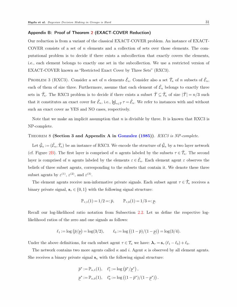
Hązła et al. Bayesian Decision Making in Groups is Hard 31
Appendix B: Proof of Theorem 2 (EXACT-COVER Reduction)
Our reduction is from a variant of the classical EXACT-COVER problem. An instance of EXACT-
COVER consists of a set of n elements and a collection of sets over those elements. The com-
putational problem is to decide if there exists a subcollection that exactly covers the elements,
i.e., each element belongs to exactly one set in the subcollection. We use a restricted version of
EXACT-COVER known as “Restricted Exact Cover by Three Sets” (RXC3).
Problem 3 (RXC3). Consider a set of n elements En. Consider also a set Tn of n subsets of En,
each of them of size three. Furthermore, assume that each element of En belongs to exactly three
sets in Tn. The RXC3 problem is to decide if there exists a subset T ⊆ Tn of size |T |= n/3 such
that it constitutes an exact cover for En, i.e.,⊎τ∈T τ = En. We refer to instances with and without
such an exact cover as YES and NO cases, respectively.
Note that we make an implicit assumption that n is divisible by three. It is known that RXC3 is
NP-complete.
Theorem 8 (Section 3 and Appendix A in Gonzalez (1985)). RXC3 is NP-complete.
Let Gn := (En, Tn) be an instance of RXC3. We encode the structure of Gn by a two layer network
(cf. Figure 2B). The first layer is comprised of n agents labeled by the subsets τ ∈ Tn. The second
layer is comprised of n agents labeled by the elements ε ∈ En. Each element agent ε observes the
beliefs of three subset agents, corresponding to the subsets that contain it. We denote these three
subset agents by ε(1), ε(2), and ε(3).
The element agents receive non-informative private signals. Each subset agent τ ∈ Tn receives a
binary private signal, sτ ∈ 0,1 with the following signal structure:
Pτ,1(1) = 1/2 =: p, Pτ,0(1) = 1/3 =: p.
Recall our log-likelihood ratio notation from Subsection 2.2. Let us define the respective log-
likelihood ratios of the zero and one signals as follows:
`1 := log(p/p)
= log(3/2), `0 := log((1− p)/(1− p)
)= log(3/4).
Under the above definitions, for each subset agent τ ∈ Tn we have: λτ = sτ (`1− `0) + `0.
The network contains two more agents called κ and i. Agent κ is observed by all element agents.
She receives a binary private signal sκ with the following signal structure:
p? := Pκ,1(1), `?1 := log(p?/p?
),
p? := Pκ,0(1), `?0 := log((1− p?)/(1− p?)
).
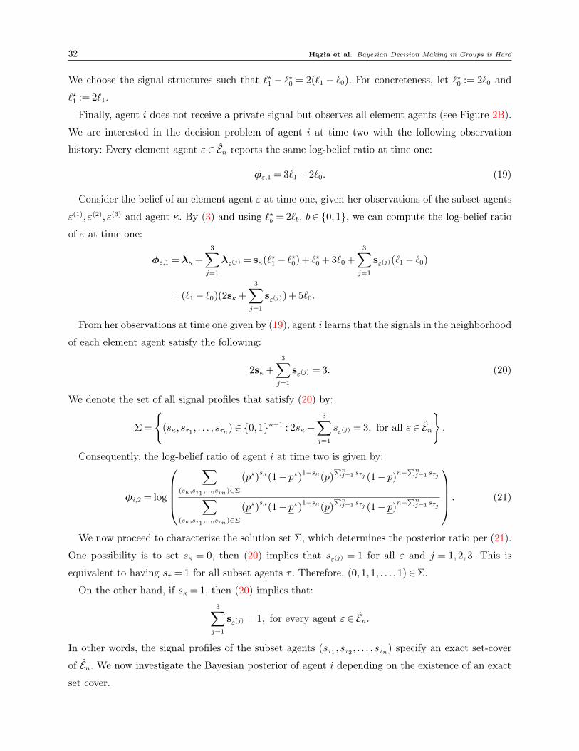
32 Hązła et al. Bayesian Decision Making in Groups is Hard
We choose the signal structures such that `?1 − `?0 = 2(`1 − `0). For concreteness, let `?0 := 2`0 and
`?1 := 2`1.
Finally, agent i does not receive a private signal but observes all element agents (see Figure 2B).
We are interested in the decision problem of agent i at time two with the following observation
history: Every element agent ε∈ En reports the same log-belief ratio at time one:
φε,1 = 3`1 + 2`0. (19)
Consider the belief of an element agent ε at time one, given her observations of the subset agents
ε(1), ε(2), ε(3) and agent κ. By (3) and using `?b = 2`b, b∈ 0,1, we can compute the log-belief ratio
of ε at time one:
φε,1 =λκ +3∑j=1
λε(j) = sκ(`?1− `?0) + `?0 + 3`0 +3∑j=1
sε(j)(`1− `0)
= (`1− `0)(2sκ +3∑j=1
sε(j)) + 5`0.
From her observations at time one given by (19), agent i learns that the signals in the neighborhood
of each element agent satisfy the following:
2sκ +3∑j=1
sε(j) = 3. (20)
We denote the set of all signal profiles that satisfy (20) by:
Σ =
(sκ, sτ1 , . . . , sτn)∈ 0,1n+1 : 2sκ +
3∑j=1
sε(j) = 3, for all ε∈ En
.
Consequently, the log-belief ratio of agent i at time two is given by:
φi,2 = log
∑
(sκ,sτ1 ,...,sτn )∈Σ
(p?)sκ(1− p?)1−sκ(p)
∑nj=1 sτj (1− p)n−
∑nj=1 sτj
∑(sκ,sτ1 ,...,sτn )∈Σ
(p?)sκ(1− p?)1−sκ(p)
∑nj=1 sτj (1− p)n−
∑nj=1 sτj
. (21)
We now proceed to characterize the solution set Σ, which determines the posterior ratio per (21).
One possibility is to set sκ = 0, then (20) implies that sε(j) = 1 for all ε and j = 1,2,3. This is
equivalent to having sτ = 1 for all subset agents τ . Therefore, (0,1,1, . . . ,1)∈Σ.
On the other hand, if sκ = 1, then (20) implies that:3∑j=1
sε(j) = 1, for every agent ε∈ En.
In other words, the signal profiles of the subset agents (sτ1 , sτ2 , . . . , sτn) specify an exact set-cover
of En. We now investigate the Bayesian posterior of agent i depending on the existence of an exact
set cover.

Hązła et al. Bayesian Decision Making in Groups is Hard 33
B.1. Bayesian Posterior in the NO Case:
If we are in a NO case of the RXC3 problem, then the instance Gn = (En, Tn) does not have an exact
set cover. Therefore, the solution set Σ is a singleton Σ = (0,1, . . . ,1) and (21) becomes:
φi,2 = log
((1− p?)(p)n
(1− p?)(p)n
)= 2`0 +n`1 = 2`0 +n log(3/2)>Ω(n),
and consequently µi,2(0) = 1/(1 + eφi,2)< exp(−Ω(n)).
B.2. Bayesian Posterior in the YES Case:
If we are in a YES case of the RXC3 problem, then there exists at least one exact cover of Enconsisting of n/3 sets from Tn. Let s′ = (sκ, sτ1 , . . . , sτn)∈Σ be a signal configuration corresponding
to such an exact cover. Let us also denote the corresponding random profile of private signals by
s = (sκ, sτ1 , . . . , sτn). The contribution of s to the Bayesian posterior of agent i can be calculated as:
P1s = s′= (p?)(p)n/3(1− p)2n/3= (p?)qn,
P0s = s′= (p?)(p)n/3(1− p)2n/3= (p?)qn,
where q := (p)1/3(1− p)2/3= 1/2 and q := (p)1/3(1− p)2/3 ≈ 0.529134.
Let N ≥ 1 be the number of exact covers of Gn. Then, we can use p= q to compute:
φi,2 = log
(N · p? · qn + (1− p?) · pn
N · p? · qn + (1− p?) · pn
)< log
(O(N · p? · qn)
N · p? · qn
)≤ nˆ+O(1) ≤−Ω(n),
where ˆ:= log(q/q)< 0. Consequently, µi,2(1) = exp(φi,2)/(1 + exp(φi,2))< exp(−Ω(n)).
All in all, from B.1 and B.2 we conclude that agent i cannot determine whether her Bayesian
posterior concentrates on state zero or state one unless she can solve the NP-hard RXC3 EXACT-
COVER variant.
Appendix C: I.I.D. Signals
Following Subsection 3.5, we explain how to modify our two reductions (VERTEX-COVER and
EXACT-COVER), in Appendices A and B, to work with i.i.d. private signals for all agents.
C.1. VERTEX-COVER
Recall that we need to modify our construction such that all agents have signal structures of vertex
agents, with p= 0.4, p= 0.3 and respective log-likelihood ratios `1 = log(p/p) = log(4/3), and `0 =
log((1− p)/(1− p)) = log(6/7).
The reduction relies on an auxiliary agent κ whose signal log-likelihood ratio is given by λκ(0) =
−cn for some constant c > 0. Since agent κ is directly observed by agent i, all we need to do is to
replace κ with a number of i.i.d. agents with the vertex agent signal structure providing a similar
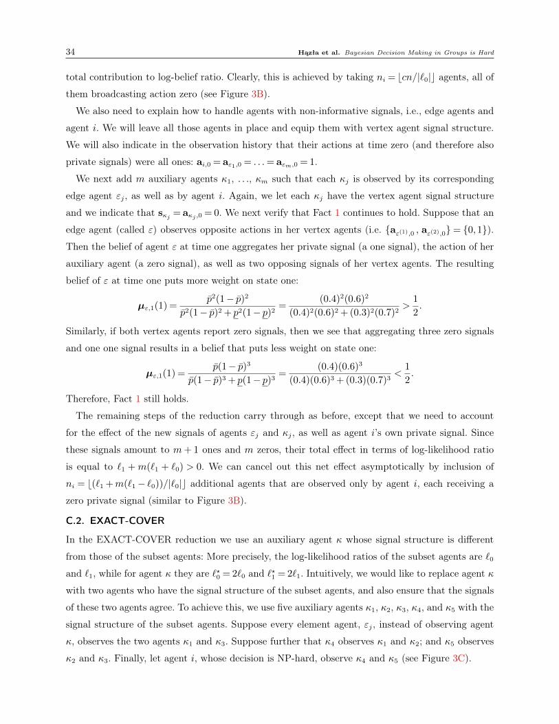
34 Hązła et al. Bayesian Decision Making in Groups is Hard
total contribution to log-belief ratio. Clearly, this is achieved by taking ni = bcn/|`0|c agents, all ofthem broadcasting action zero (see Figure 3B).
We also need to explain how to handle agents with non-informative signals, i.e., edge agents and
agent i. We will leave all those agents in place and equip them with vertex agent signal structure.
We will also indicate in the observation history that their actions at time zero (and therefore also
private signals) were all ones: ai,0 = aε1,0 = . . .= aεm,0 = 1.
We next add m auxiliary agents κ1, . . ., κm such that each κj is observed by its corresponding
edge agent εj, as well as by agent i. Again, we let each κj have the vertex agent signal structure
and we indicate that sκj = aκj ,0 = 0. We next verify that Fact 1 continues to hold. Suppose that an
edge agent (called ε) observes opposite actions in her vertex agents (i.e. aε(1),0 , aε(2),0= 0,1).Then the belief of agent ε at time one aggregates her private signal (a one signal), the action of her
auxiliary agent (a zero signal), as well as two opposing signals of her vertex agents. The resulting
belief of ε at time one puts more weight on state one:
µε,1(1) =p2(1− p)2
p2(1− p)2 + p2(1− p)2=
(0.4)2(0.6)2
(0.4)2(0.6)2 + (0.3)2(0.7)2>
1
2.
Similarly, if both vertex agents report zero signals, then we see that aggregating three zero signals
and one one signal results in a belief that puts less weight on state one:
µε,1(1) =p(1− p)3
p(1− p)3 + p(1− p)3=
(0.4)(0.6)3
(0.4)(0.6)3 + (0.3)(0.7)3<
1
2.
Therefore, Fact 1 still holds.
The remaining steps of the reduction carry through as before, except that we need to account
for the effect of the new signals of agents εj and κj, as well as agent i’s own private signal. Since
these signals amount to m+ 1 ones and m zeros, their total effect in terms of log-likelihood ratio
is equal to `1 + m(`1 + `0) > 0. We can cancel out this net effect asymptotically by inclusion of
ni = b(`1 +m(`1− `0))/|`0|c additional agents that are observed only by agent i, each receiving a
zero private signal (similar to Figure 3B).
C.2. EXACT-COVER
In the EXACT-COVER reduction we use an auxiliary agent κ whose signal structure is different
from those of the subset agents: More precisely, the log-likelihood ratios of the subset agents are `0and `1, while for agent κ they are `?0 = 2`0 and `?1 = 2`1. Intuitively, we would like to replace agent κ
with two agents who have the signal structure of the subset agents, and also ensure that the signals
of these two agents agree. To achieve this, we use five auxiliary agents κ1, κ2, κ3, κ4, and κ5 with the
signal structure of the subset agents. Suppose every element agent, εj, instead of observing agent
κ, observes the two agents κ1 and κ3. Suppose further that κ4 observes κ1 and κ2; and κ5 observes
κ2 and κ3. Finally, let agent i, whose decision is NP-hard, observe κ4 and κ5 (see Figure 3C).
Hązła et al. Bayesian Decision Making in Groups is Hard 35
The private signals of κ4 and κ5 can be set arbitrarily. Suppose that the belief reports of κ4 and
κ5 at time two implies the following log-belief ratios: φκ4,2 =λκ4 + `0 + `1 and φκ5,2 =λκ5 + `0 + `1.
From observing κ4, agent i learns that the sum of the log-likelihood ratios of the signals of κ1 and
κ2 is `0 + `1; equivalently, κ1 and κ2 have received opposite signals. Similarly, from observing κ5
agent i learns that κ2 and κ3 have received opposite signals. Therefore, signals of κ1 and κ3 must
agree. Observing κ1 and κ3 has the same effect on beliefs of the element agents as observing the
single auxiliary agent κ with two times the signal strength. Note that agent i is influenced by what
she learned about signals of λκ2 ,λκ4 and λκ5 , but this influence is of the order O(1) and therefore
does not affect our analysis of Bayesian posteriors in Appendix B.
As for the agents without private signals, i.e., agent i and element agents, the modifications are
quite simple. Again, we assume that all these agents have the same signal structure as the subset
agents, and that they report beliefs at time zero consistent with zero private signals. This introduces
a negative shift equal to (n+ 1)`0 in the log-belief ratio of agent i, which can be asymptotically
canceled by adding ni = b(n+ 1)|`0|/`1c more auxiliary agents that report ones as their signals and
are observed only by agent i (similar to Figure 3B).
Appendix D: Noisy Actions
As described in Subsection 3.6, let us consider the following noisy variant of the binary action
model: For each computed action ai,t, the neighboring agents observe the same action a′i,t = ai,t
with probability 1− δ and the flipped action a′i,t = 1−ai,t with probability δ, for some 0< δ < 1/2.
We want to show that Theorem 1 still holds in this model, possibly with the constants in the size
of the reduction and the exp(−Ω(n)) belief approximation factor depending on δ. To this end, we
use the same VERTEX-COVER problem and the high-level idea as the proof of Theorem 1.
Let us start with the general examination of the effect of noise on an agent τ that receives a
private signal with signal structure Pτ,1(1) = p and Pτ,0(1) = p. From the perspective of an agent
that observes τ , separating the private signal of τ and the error in its action does not matter: All
that matters is the likelihood that can be inferred from observing aτ,0. The likelihoods of the two
possible observations are as follows:
p′ := P1a′τ,0 = 1= P1aτ,0 = a′τ,0 = 1 or aτ,0 = 1−a′τ,0 = 0= p(1− δ) + (1− p)δ,
p′ := P0a′τ,0 = 0= p(1− δ) + (1− p)δ. (22)
From (22), we see that the “after-noise” signal structures are restricted to δ≤ p′, p′ ≤ 1− δ, rather
than having the full range between 0 and 1. Accordingly, we start the VERTEX-COVER reduction
by specifying the after-noise signal structures of the vertex agents as follows: p′ = 1/4 + δ/2 and

36 Hązła et al. Bayesian Decision Making in Groups is Hard
p′ = δ. It is easy to check that since p′ < p′ < 1/2 and since p′(1− p′)< p′(1− p′), an edge agent ε
observing two vertex agents, ε(1) and ε(2), still satisfies the following version of Fact 1:
aε,1 = 1 if, and only if, a′ε(1),0
= 1 or a′ε(2)
= 1. (23)
Note that aε,1 on the left-hand side is before-noise, but a′ε(1),0
and a′ε(2),0
on the right-hand side, are
after-noise. We will now proceed with the analysis of the reduction, encoding vertex covers of the
input graph Gn,m in the after-noise actions a′τ,0 of vertex agents.
Previously, for each edge of Gn,m we placed an edge agent ε observing two vertex agents, ε(1) and
ε(2), corresponding to its incident vertices in Gn,m. This time, for each edge we place k := k(n,m, δ)
agents ε(1), . . . , ε(k), each of them observing the same two vertex agents and reporting the same
noisy actions a′ε(j),1 = 1, j = 1, . . . , k to agent i (see Figure 3D). Since by (23) the before-noise actions
aε(j),1 have all been the same, after observing ε(1), . . . , ε(k) agent i concludes that exactly one of
the following is true:
• Nobody among ε(1), . . ., ε(k) has flipped her action: aε(j),1 = a′ε(j),1 = 1, j = 1, . . . , k.
• Everybody in ε(1), . . ., ε(k) has flipped her action: aε(j),1 = 1−a′ε(j),1 = 0, j = 1, . . . , k.
In the second case, we say that “an error has occurred in edge ε”. We now proceed to show that for
k large enough the probability of an error occurring in some edge is so small that the analysis of
the noisy model essentially reduces back to what we did in Appendix A.
To this end, consider the log-belief ratio of agent i at time two, as described in (12), neglecting
for the moment the influence of agent κ. Let Σ := τ ∈ V : a′τ,0 = 1. Following Appendix A, agent i
concludes that either Σ forms a vertex cover of Gn,m or an error has occurred in at least one edge.
Let E denote the event that at least one error has occurred and let ¬E denote its complement. If
we want to, for example, upper-bound φi,2 in the NO case, we can write:
φi,2 = log
(µi,2(1)
µi,2(0)
)≤ log
(P1Σ is a vertex cover∧¬E+P1E | hi,2
P0Σ is a vertex cover∧¬E
), (24)
where we drop the error probability term (P0E | hi,2) in the denominator to obtain an upper-
bound. We now note that, by union bound and other elementary considerations, the error probability
can be bounded by:
P1E | hi,2 ≤mδk(δk + (1− δ)k
)m−1=m
(δk + (1− δ)k
(1− δ)k
)m−1(δ
1− δ
)k(1− δ)km
≤m2m(
δ
1− δ
)k(1− δ)km ≤ (1/8 + δ/4)n(1− δ)km = (p′/2)n(1− δ)km
= (1/2)nP1∀τ : a′τ,0 = 1∧¬E≤ (1/2)nP1Σ is a vertex cover∧¬E, (25)
where in the first line we use the fact that conditioned on observation history hi,2, for each edge
either 0 or k flips has occurred. In the second line, we make m2m (δ/(1− δ))k ≤ (1/8 + δ/4)n by
choosing k to be (polynomially) large enough — recall δ/(1− δ)< 1.
Hązła et al. Bayesian Decision Making in Groups is Hard 37
Taken together, (24) and (25) imply that, up to a tiny exp(−Ω(n)) factor, the value of φi,2 is
almost the same as that computed in (12). Therefore, we can use the same computation as in (13)
to establish a linear lower-bound on φi,2. The YES case is handled very similarly.
Finally, it remains to account for agent κ. This is done in basically the same way as in Sub-
section 3.5: We replace agent κ with the strong log-likelihood ratio λκ(0) = −cn by⌊cnδ′
⌋agents
with the after-noise log-likelihood ratio λ′κj (0) =−δ′ for appropriately small δ′ = δ′(δ), all reporting
action zero at time zero. This concludes the description of our modification in the noisy model.
Appendix E: Complexity of Bayesian Decisions Using Algorithm 1: IEIS
Suppose that agent i has reached her t-th decision in a general network structure. Given her infor-
mation at time t, for all s = (s1, . . . , sn) ∈ S1 × . . .×Sn and any j ∈ N τi , τ = t+ 1, t, . . . ,1 she has
to update I(j, t− τ, s) into I(j, t+ 1− τ, s)⊂ I(j, t− τ, s). If τ = t+ 1 then agent j ∈N τi is being
considered for the first time at the t-th step and I(j,0, s) = sj×∏k 6=j Sk is initialized without any
calculations. However if τ ≤ t, then I(j, t− τ, s) can be updated into I(j, t+ 1− τ, s)⊂I(j, t− τ, s)
only by verifying the condition ak,t−τ (s′) = ak,t−τ (s) for every s′ ∈ I(j, t − τ, s) and k ∈ Nj: any
s′ ∈ I(j, t− τ, s) that violates this condition for some k ∈ Nj is eliminated and I(j, t+ 1− τ, s) is
thus obtained by pruning I(j, t− τ, s).
Verification of ak,t−τ (s′) = ak,t−τ (s) involves calculations of ak,t−τ (s′) and ak,t−τ (s) according to
(6). The latter requires the addition of card(I(k, t− τ, s)) product terms uk(ak, θ′) Pθ′(s′) ν(θ′) =
uk(ak, θ′) P1,θ′(s
′1) . . . Pn,θ′(s′n) ν(θ′) for each s′ ∈ I(k, t − τ, s), θ′ ∈ Θ, and ak ∈ Ak to evaluate
the left hand-side of (6). Hence, we can estimate the total number of additions and multiplications
required for calculation of each conditional action ak,t−τ (s) as A. (n + 2) .m . card(I(k, t − τ, s)),
where m := card(Θ) and A = maxk∈[n] card(Ak). Hence the total number of additions and multi-
plications undertaken by agent i at time t for determining actions ak,t−τ (s) can be estimated as
follows:
C1 :=A. (n+ 2) . card(Θ) .∑j∈N ti
∑k∈Nj
card(I(k, t− dist(j, i), s))≤A. (n+ 2) . n .Mn−1 .m, (26)
where we upper-bound the cardinality of the union of the higher-order neighborhoods of agent i by
the total number of agents: card(N t+1i )≤ n and use the inclusion relationship I(k, t−dist(j, i), s)⊂
I(k,0, s) = sk ×∏j 6=k Sj to upper-bound card(I(k, t − dist(j, i), s)) by Mn−1 where M is the
largest cardinality of finite signal spaces, Sj, j ∈ [n] . As the above calculations are performed at
every signal profile s ∈ S1× . . .Sn the total number of calculations (additions and multiplications)
required for the Bayesian decision at time t, denoted by Ct, can be bounded as follows:
A.Mn ≤Ct ≤A. (n+ 2) . n .M 2n−1 .m, (27)

38 Hązła et al. Bayesian Decision Making in Groups is Hard
where on the right-hand side, we apply (26) for each of the Mn signal profiles. In particular, the
calculations grow exponential in the number of agents n. Once agent i calculates the actions ak,t−τ (s)
for all k ∈ Nj she can then update the possible signal profiles I(j, t − τ, s), following step 2(a)ii
of Algorithm 1, to obtain I(j, t+ 1− τ, s) for all j ∈ N ti and any s ∈ S1 × . . .× Sn. This in turn
enables her to calculate the conditional actions of her neighbors aj,t(s) at every signal profile and
to eliminate any s at which the conditional action aj,t(s) does not agree with the observed action
aj,t, for some j ∈Ni. She can thus update her list of possible signal profiles from I i,t to I i,t+1 and
adopt the corresponding Bayesian belief µi,t+1 and action ai,t+1. The latter involves an additional
(n + 2)mA · card(I i,t+1) additions and multiplication which are, nonetheless, dominated by the
number of calculations required in (27) for the simulation of other agents’ actions at every signal
profile.
Appendix F: Computational Complexity of Algorithm 2: IEIS-TRANSITIVE
According to (I2), in a transitive structure at time t agent i has access to the list of possible private
signals for each of her neighbors: Sj,t, j ∈Ni given their observations up until that point in time.
The possible signal set Sj,t for each agent j ∈Ni is calculated based on the actions taken by others
and observed by agent j until time t− 1 together with possible private signals that can explain
her history of choices: aj,0, aj,1, and so on up until her most recent choice which is aj,t. At time
t, agent i will have access to all the observations of every agent in her neighborhood and can vet
their most recent choices aj,t against their observations to eliminate the incompatible private signals
from the possible set Sj,t and obtain an updated list of possible signals Sj,t+1 for each of her
neighbors j ∈Ni. This pruning is achieved by calculating aj,t(sj) given Ij,t(sj) = sj×∏k∈Nj
Sj,t
for each sj ∈Sj,t and removing any incompatible sj that violates the condition aj,t = aj,t(sj); thus
obtaining the pruned set Sj,t+1. The calculation of aj,t(sj) given Ij,t(sj) = sj ×∏k∈Nj
Sj,t is
performed according to (6) but the decomposition of the possible signal profiles based on the relation
Ij,t(sj) = sj×∏k∈Nj
Sj,t together with the independence of private signals across different agents
help reduce the number of additions and multiplications involved as follows:
Aj(Ij,t(sj)) = arg maxaj∈Aj
∑θ′∈Θ
uj(aj, θ′)
∑s′∈Ij,t(sj)
Pθ′(s′)ν(θ′)∑θ′′∈Θ
∑s′∈Ij,t(sj)
Pθ′′(s′)ν(θ′′)
= arg maxaj∈Aj
∑θ′∈Θ
uj(aj, θ′)
Pθ′(sj)∏k∈Nj
∑sk∈Sk,t
Pθ′(sk)ν(θ′)∑θ′′∈Θ Pθ′′(sj)
∏k∈Nj
∑sk∈Sk,t
Pθ′′(sk)ν(θ′′).
Hązła et al. Bayesian Decision Making in Groups is Hard 39
Hence, the calculation of the conditionally feasible action aj,t(sj) for each sj ∈Sj,t can be achieved
through card(Θ) A∑
k∈Njcard(Sk,t) additions and card(Θ) (card(Nj) + 2)A multiplications; sub-
sequently, the total number of additions and multiplications required for agent i to update the
possible private signals of each of her neighbor can be estimated as follows:
A∑j∈Ni
card(Θ)card(Sj,t)
∑k∈Nj
card(Sk,t) + card(Nj) + 2
≤An2M 2m+An2Mm+ 2nMmA, (28)
where M , n, m and A are as in (27). After updating her lists for the possible signal pro-
files of all her neighbors, the agent can refine her list of possible signal profiles I i,t+1 = si ×∏j∈Ni
Sj,t+1 and determine her belief µi,t+1 and refined choice ai,t+1. The latter is achieved through
an extra card(Θ)A∑
j∈Nicard(Sj,t+1) additions and card(Θ)A (card(Ni) + 2) multiplications, which
are dominated by the required calculations in (28). Most notably, the computations required of
the agent for determining her Bayesian choices in a transitive network increase polynomially in the
number of agents n, whereas in a general network structure using IEIS these computations increase
exponentially fast in the number of agents n.
Appendix G: Proof of Proposition 1 (Graphical Condition for Transparency)
The proof follows by induction on t, i.e. by considering the agents whose information reach agent
i for the first time at t. The claim is trivially true at time one, since agent i can always infer the
likelihoods of the private signals of each of her neighbors by observing their beliefs at time one. Now
consider the belief of agent i at time t, the induction hypothesis implies that φi,t−1 =∑
k∈N t−1i
λk,
as well as φj,t−1 =∑
k∈N t−1j
λk and φj,t−2 =∑
k∈N t−2j
λk for all j ∈ Ni. To form her belief at time
t (or equivalently its log-belief ratio φi,t), agent i should consider her most recent information
φj,t−1 =∑
k∈N t−1j
λk, j ∈ Ni and use that to update her current belief φi,t−1 =∑
k∈N t−1i
λk. To
prove the induction claim, it suffices to show that agent i has enough information to calculate the
sum of log-likelihood ratios of all signals in her t-radius ego-net, N ti ; i.e. to form φi,t =
∑k∈N ti
λk.
This is the best possible belief that she can hope to achieve at time t, and it is the same as her
Bayesian posterior, had she direct access to the private signals of all agents in her t-radius ego-net.
To this end, by using her knowledge of φj,t−1 and φj,t−2 she can form:
φj,t−1 =φj,t−1−φj,t−2 =∑
k∈N t−1j
λk,
for all j ∈ Ni. Since, φi,t−1 =∑
k∈N t−1i
λk by the induction hypothesis, the efficient belief φi,t =∑k∈N ti
λk can be calculated if and only if,
φi,t =φi,t−φi,t−1 =∑k∈N ti
λk, (29)
40 Hązła et al. Bayesian Decision Making in Groups is Hard
can be computed. In the above formulation φi,t is an innovation term, representing the information
that agent i learns from her most recent observations at time t. We now show that under the
assumption that any agent with multiple paths to an agent i is directly observed by her, the
innovation term in (29) can be constructed from the knowledge of φj,t−1 =∑
k∈N t−1j
λk, and φj,t−2 =∑k∈N t−2
jλk for all j ∈Ni; indeed, we show that:
φi,t =∑j∈Ni
φj,t−1−∑
k∈Ni∩Nt−1j
φk,0
, for all t > 1. (30)
Consider any k ∈N ti , these are all agents which are at distance exactly t, t > 1, from agent i, and no
closer to her. No such k ∈N ti is a direct neighbor of agent i and the structural assumption therefore
implies that there is a unique neighbor of agent i, call this unique neighbor jk ∈ Ni, satisfying
k ∈ N t−1jk
. On the other hand, consider any j ∈ Ni and some k ∈ N t−1j , contributing λk to φj,t−1.
Such an agent k is either a neighbor of i or else at distance exactly t > 1 from agent i and therefore
k ∈ N ti , and element j would be the unique neighbor jk ∈ Ni satisfying k ∈ N t−1
jk. Subsequently,
using the notation ] for disjoint unions, we can partition N ti as follows:
N ti =]j∈NiN
t−1j \
(N t−2j ∪Ni
),
and therefore we can rewrite the left-hand side of (29) as follows:
φi,t =∑k∈N ti
λk =∑
k∈]j∈NiN t−1j \(N t−2
j ∪Ni)
λk =∑j∈Ni
∑k∈N t−1
j \
(N t−2j ∪Ni)
λk
=∑j∈Ni
∑k∈N t−1
j
λk−∑
k∈Ni∩Nt−1j
λk
=∑j∈Ni
φj,t−1−∑
k∈Ni∩Nt−1j
φk,0
,
as claimed in (30), completing the proof.
Notes
1. Technically we showed coNP-hardness, i.e., our reduction mapped instances with small vertex cover onto GROUP-
DECISION instances with θ = 0 and instances with only large vertex covers onto GROUP-DECISION with θ = 1.
However, due to the symmetric nature of GROUP-DECISION, NP-hardness is immediately obtained by inverting
the meanings of 0 and 1 labels of states and private signals. In particular, since GROUP-DECISION at t= 2 is both
NP-hard and coNP-hard, it is likely to be strictly harder than NP-complete (see Arora and Barak (2009)).
2. In the context of Subsection 3.1, one might argue that in the absence of a common prior there is no fixed distribution
of signals over which to obtain an average-case hardness result. Notwithstanding, the worst-case issue remains relevant
because the observation history is now exponentially unlikely according to each agent’s own prior.

Hązła et al. Bayesian Decision Making in Groups is Hard 41
3. We note that Algorithm 0 can be implemented to use space that is polynomial in the number of agents and time t
(assuming fixed state set Θ, signal sets Si and action sets Ai). In the binary action model this matches our PSPACE-
hardness results obtained in the follow-up paper Hązła et al. (2019).
4. This is a fundamental aspect of inference problems in observational learning (in learning from other actors): similar
to responsiveness that Ali (2018) defines as a property of the utility functions to determine whether players’ beliefs
can be inferred from their actions, transparency in our belief exchange setup is defined as a property of the graph
structure (see Remark 2 on why transparency is a structural property) which determines to what extent other players’
private signals can be inferred from observing the neighboring beliefs.
AcknowledgmentsThis work was partially supported by awards ONR N00014-16-1-2227, NSF CCF-1665252 and ARO MURIs
W911NF-12-1-0509, W911NF-19-0217 and by a Vannevar Bush Fellowship.
References
Aaronson S (2005) The complexity of agreement. Proceedings of the thirty-seventh annual ACM symposium
on Theory of computing, 634–643 (ACM).
Acemoglu D, Bimpikis K, Ozdaglar A (2014) Dynamics of information exchange in endogenous social net-
works. Theoretical Economics 9(1):41–97.
Acemoglu D, Dahleh MA, Lobel I, Ozdaglar A (2011) Bayesian learning in social networks. The Review of
Economic Studies 78(4):1201–1236.
Acemoglu D, Ozdaglar A (2011) Opinion dynamics and learning in social networks. Dynamic Games and
Applications 1(1):3–49, ISSN 2153-0793.
Ali SN (2018) Herding with costly information. Journal of Economic Theory 175:713–729.
Arieli I, Babichenko Y, Mueller-Frank M (2019a) Naive learning through probability matching. Conference
on Economics and Computation, 553 (ACM), ISBN 978-1-4503-6792-9.
Arieli I, Babichenko Y, Shlomov S (2019b) Robust non-Bayesian social learning. Conference on Economics
and Computation, 549–550 (ACM), ISBN 978-1-4503-6792-9.
Arora S, Barak B (2009) Computational Complexity: A Modern Approach (New York, NY, USA: Cambridge
University Press), 1st edition, ISBN 0521424267, 9780521424264.
Arora S, Barak B, Brunnermeier M, Ge R (2011) Computational complexity and information asymmetry in
financial products. Communications of the ACM 54(5):101–107, ISSN 0001-0782.
Aumann RJ (1976) Agreeing to disagree. The annals of statistics 1236–1239.
Bala V, Goyal S (1998) Learning from neighbours. The Review of Economic Studies 65(3):595–621.
Banerjee AV (1992) A simple model of herd behavior. The Quarterly Journal of Economics 107(3):797–817.
42 Hązła et al. Bayesian Decision Making in Groups is Hard
Bikhchandani S, Hirshleifer D, Welch I (1998) Learning from the behavior of others: Conformity, fads, and
informational cascades. The Journal of Economic Perspectives 12(3):pp. 151–170, ISSN 08953309.
Blackwell D, Dubins L (1962) Merging of opinions with increasing information. The Annals of Mathematical
Statistics 33:882 – 886.
Bogdanov A, Trevisan L, et al. (2006) Average-case complexity. Foundations and Trends in Theoretical
Computer Science 2(1):1–106.
Dasaratha K, Golub B, Hak N (2018) Social learning in a dynamic environment. arXiv preprint
arXiv:1801.02042 .
DeGroot MH (1974) Reaching a consensus. Journal of American Statistical Association 69:118–121.
DeMarzo PM, Vayanos D, Zwiebel J (2003) Persuasion bias, social influence, and unidimensional opinions.
The Quarterly Journal of Economics 118:909–968.
Eyster E, Rabin M (2014) Extensive imitation is irrational and harmful. The Quarterly Journal of Economics
129(4):1861–1898.
Fudenberg D, Maskin E (1986) The folk theorem in repeated games with discounting or with incomplete
information. Econometrica 54(3):533–554.
Gale D, Kariv S (2003) Bayesian learning in social networks. Games and Economic Behavior 45:329–346.
Geanakoplos JD, Polemarchakis HM (1982) We can’t disagree forever. Journal of Economic Theory
28(1):192–200.
Golub B, Jackson MO (2010) Naïve Learning in Social Networks and the Wisdom of Crowds. American
Economic Journal: Microeconomics 2(1):112–149.
Gonzalez TF (1985) Clustering to minimize the maximum intercluster distance. Theoretical Computer Science
38:293–306, ISSN 0304-3975.
Harel M, Mossel E, Strack P, Tamuz O (2014) When more information reduces the speed of learning Working
paper.
Hązła J, Jadbabaie A, Mossel E, Rahimian MA (2019) Reasoning in Bayesian opinion exchange networks
is PSPACE-hard. Conference on Learning Theory, volume 99 of Proceedings of Machine Learning
Research, 1614–1648 (PMLR).
Jadbabaie A, Molavi P, Sandroni A, Tahbaz-Salehi A (2012) Non-Bayesian social learning. Games and
Economic Behavior 76(1):210 – 225.
Kanoria Y, Tamuz O (2013) Tractable bayesian social learning on trees. Selected Areas in Communications,
IEEE Journal on 31(4):756–765.
Khot S, Minzer D, Safra M (2018) Pseudorandom Sets in Grassmann Graph have Near-Perfect Expansion.
ECCC Technical Report TR18-078 .

Hązła et al. Bayesian Decision Making in Groups is Hard 43
Krishnamurthy V, Hoiles W (2014) Online reputation and polling systems: Data incest, social learning, and
revealed preferences. IEEE Transactions on Computational Social Systems 1(3):164–179.
Kwisthout J (2011) The Computational Complexity of Probabilistic Inference. Technical Report ICIS–
R11003, Radboud University Nijmegen.
Lehrer E, Smorodinsky R (1996) Merging and learning. Lecture Notes-Monograph Series 147–168.
Li W, Tan X (2018) Locally bayesian learning in networks. Working paper .
Molavi P, Tahbaz-Salehi A, Jadbabaie A (2018) A theory of non-bayesian social learning. Econometrica
86(2):445–490.
Mossel E, Mueller-Frank M, Sly A, Tamuz O (2018) Social learning equilibria. Proceedings of the 2018 ACM
Conference on Economics and Computation, 639–639 (ACM).
Mossel E, Olsman N, Tamuz O (2016) Efficient bayesian learning in social networks with gaussian estimators.
2016 54th Annual Allerton Conference on Communication, Control, and Computing (Allerton), 425–
432 (IEEE).
Mossel E, Sly A, Tamuz O (2014) Asymptotic learning on bayesian social networks. Probability Theory and
Related Fields 158(1-2):127–157, ISSN 0178-8051.
Mossel E, Sly A, Tamuz O (2015) Strategic learning and the topology of social networks. Econometrica
83(5):1755–1794.
Mossel E, Tamuz O (2013) Making consensus tractable. ACM Transactions on Economics and Computation
1(4):20.
Mossel E, Tamuz O (2017) Opinion exchange dynamics. Probability Surveys 14:155–204.
Mueller-Frank M (2013) A general framework for rational learning in social networks. Theoretical Economics
8(1):1–40.
Mueller-Frank M, Neri C (2017) A general analysis of boundedly rational learning in social networks. Available
at SSRN 2933411 .
Papadimitriou CH, Tsitsiklis JN (1987) The complexity of markov decision processes. Mathematics of oper-
ations research 12(3):441–450.
Rosenberg D, Solan E, Vieille N (2009) Informational externalities and emergence of consensus. Games and
Economic Behavior 66(2):979–994.
Smith L, Sørensen P (2000) Pathological outcomes of observational learning. Econometrica 68(2):371–398.
Velupillai K (2000) Computable economics: the Arne Ryde memorial lectures, volume 5 (Oxford University
Press on Demand).