bayesian decision theory - svcl · bayesian decision theory recall that we have • y – state of...
TRANSCRIPT
Bayesian decision theory
Nuno Vasconcelos ECE Department, UCSDp ,
Bayesian decision theoryrecall that we have• Y – state of the worldY – state of the world• X – observations• g(x) – decision function• L[g(x),y] – loss of predicting y with g(x)
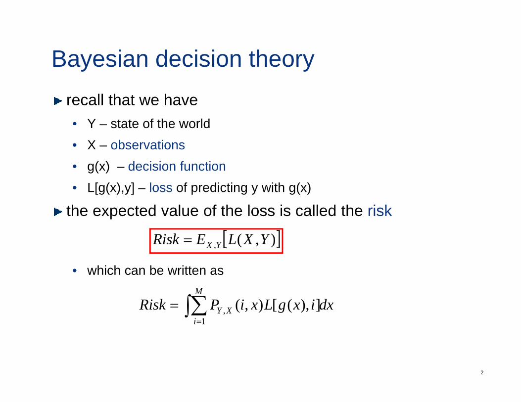
the expected value of the loss is called the risk
• which can be written as
[ ]),(, YXLERisk YX=
dxixgLxiPRiskM
iXY∫∑
=
= ]),([),(1
,
2
Bayesian decision theory PY|X(1|x) = 1
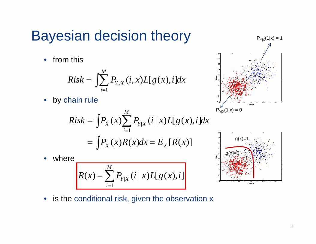
• from thisM
∫∑• by chain rule
dxixgLxiPRiski
XY∫∑=
= ]),([),(1
,
dxixgLxiPxPRiskM
iXYX∫ ∑
=
= ]),([)|()(1
|
∫
PY|X(1|x) = 0
( ) 1
• where
)]([)()( xREdxxRxP XX == ∫M
g(x)=0
g(x)=1
• is the conditional risk given the observation x
]),([)|()(1
| ixgLxiPxRM
iXY∑
=
=
3
• is the conditional risk, given the observation x
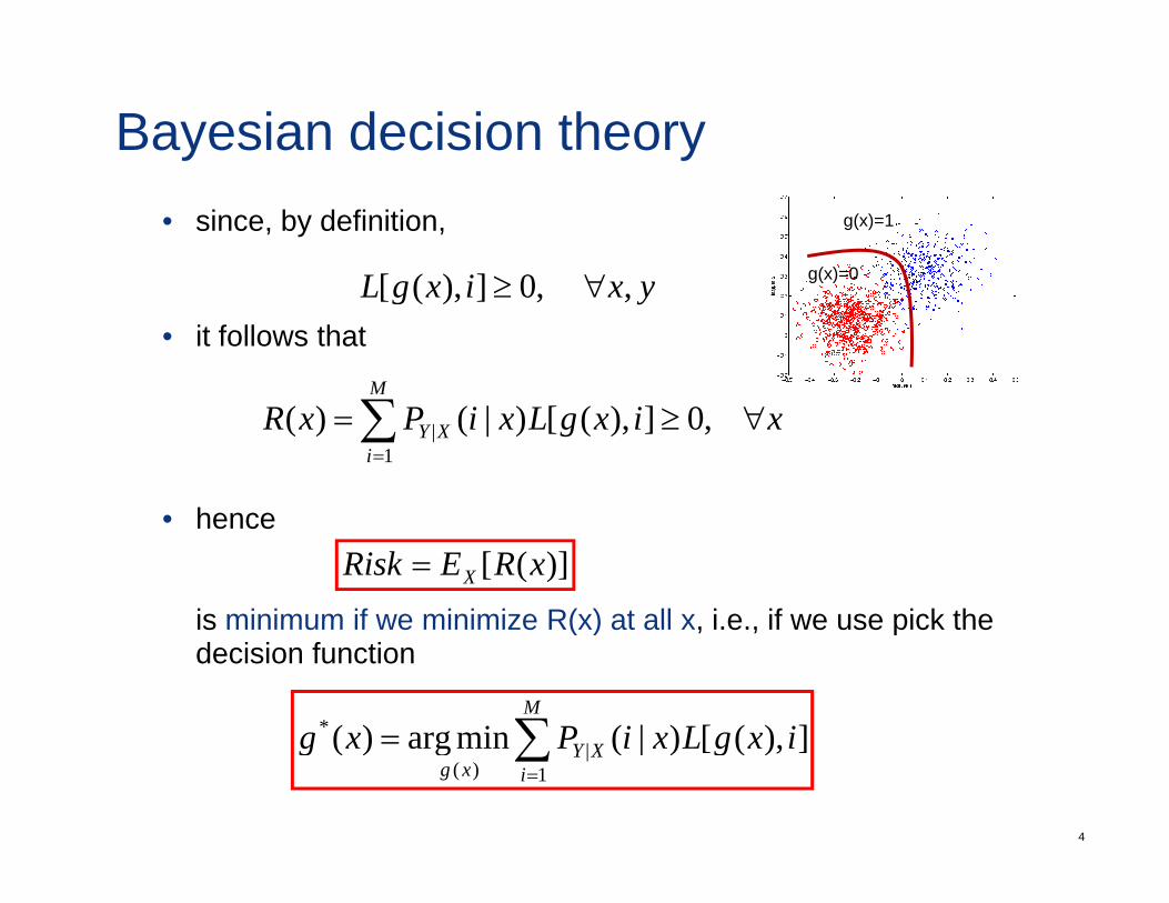
Bayesian decision theory• since, by definition,
iL 0])([ ∀≥ g(x)=0
g(x)=1
• it follows thatyxixgL , ,0]),([ ∀≥
M
g( )
h
xixgLxiPxRi
XY ∀≥=∑=
,0]),([)|()(1
|
• hence
is minimum if we minimize R(x) at all x i e if we use pick the
)]([ xRERisk X=
is minimum if we minimize R(x) at all x, i.e., if we use pick the decision function
])([)|(minarg)(* ixgLxiPxgM
∑=
4
]),([)|(minarg)(1
|)(
ixgLxiPxgi
XYxg∑=
=
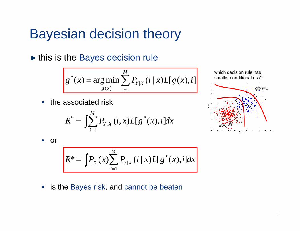
Bayesian decision theorythis is the Bayes decision rule
M which decision rule has
the associated risk
]),([)|(minarg)(1
|)(
* ixgLxiPxgM
iXY
xg∑=
=g(x)=1
which decision rule hassmaller conditional risk?
• the associated risk
dxixgLxiPRM
iXY∫∑
=
= ]),([),( *
1,
*g(x)=0
• ori=1
dxixgLxiPxPRM
∫ ∑= ])([)|()(* *
• is the Bayes risk and cannot be beaten
dxixgLxiPxPRi
XYX∫ ∑=
= ]),([)|()(*1
|
5
is the Bayes risk, and cannot be beaten
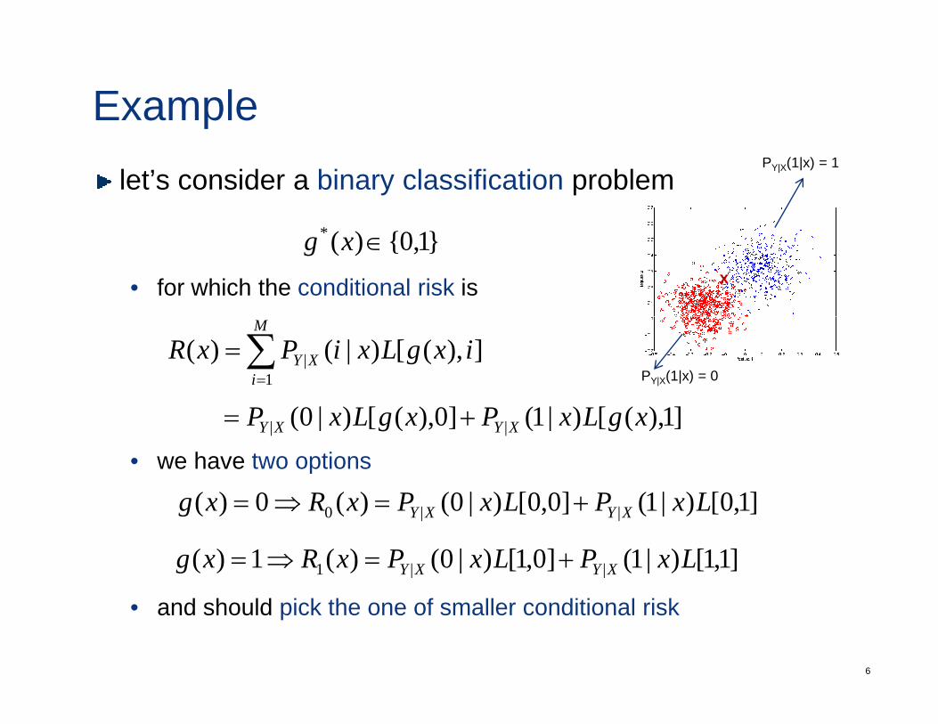
Examplelet’s consider a binary classification problem
PY|X(1|x) = 1
• for which the conditional risk is
}1,0{)(* ∈xgx
]),([)|()(1
| ixgLxiPxRM
iXY∑
=
=
]1)([)|1(]0)([)|0( LPLPPY|X(1|x) = 0
• we have two options
]1),([)|1(]0),([)|0( || xgLxPxgLxP XYXY +=
]10[)|1(]00[)|0()(0)( LxPLxPxRxg +⇒ ]1,0[)|1(]0,0[)|0()(0)( ||0 LxPLxPxRxg XYXY +=⇒=
]1,1[)|1(]0,1[)|0()(1)( ||1 LxPLxPxRxg XYXY +=⇒=
6
• and should pick the one of smaller conditional risk
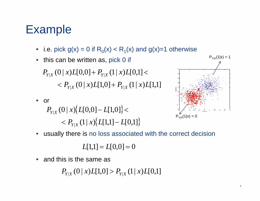
Example• i.e. pick g(x) = 0 if R0(x) < R1(x) and g(x)=1 otherwise• this can be written as, pick 0 if PY|X(1|x) = 1, p
]1,1[)|1(]0,1[)|0( ]1,0[)|1(]0,0[)|0(
||
||
LxPLxPLxPLxP
XYXY
XYXY
+<
<+
• or
],[)|(],[)|( || XYXY
{ }]0,1[]0,0[)|0(| LLxP XY <−
x
• usually there is no loss associated with the correct decision
{ }{ }]1,0[]1,1[)|1(
][][)|(
|
|
LLxP XY
XY
−<PY|X(1|x) = 0
• and this is the same as
0]0,0[]1,1[ == LL
7
]1,0[)|1(]0,1[)|0( || LxPLxP XYXY >
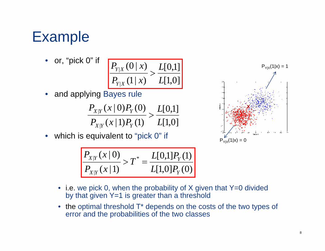
Example• or, “pick 0” if
]01[]1,0[
)|1()|0(|
LL
PxP XY >
PY|X(1|x) = 1
• and applying Bayes rule]0,1[)|1(| LxP XY
]10[)0()0|(| LPxP YYXx
• which is equivalent to “pick 0” if]0,1[]1,0[
)1()1|()0()0|(
|
|
LL
PxPPxP
YYX
YYX >
PY|X(1|x) = 0
)0(]0,1[)1(]1,0[
)1|()0|( *
|
|
Y
Y
YX
YX
PLPLT
xPxP
=>
PY|X(1|x) 0
• i.e. we pick 0, when the probability of X given that Y=0 dividedby that given Y=1 is greater than a thresholdth ti l th h ld T* d d th t f th t t f
)(],[)|(| YYX
8
• the optimal threshold T* depends on the costs of the two types of error and the probabilities of the two classes
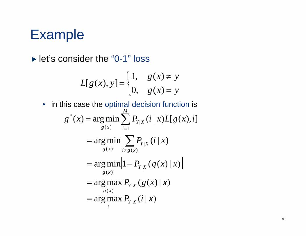
Examplelet’s consider the “0-1” loss
⎧ )(1
in this case the optimal decision function is⎩⎨⎧
=≠
=yxgyxg
yxgL)(,0)(,1
]),([
• in this case the optimal decision function is
]),([)|(minarg)(1
|)(
* ixgLxiPxgM
iXY
xg∑=
=
)|(minarg)(
|)(
xiPxgi
XYxg
∑≠
=
[ ])|)((1minarg xxgP[ ])|)((1minarg |)(
xxgP XYxg
−=
)|)((maxarg |)(
xxgP XYxg
=
9
)(g
)|(maxarg | xiP XYi
=
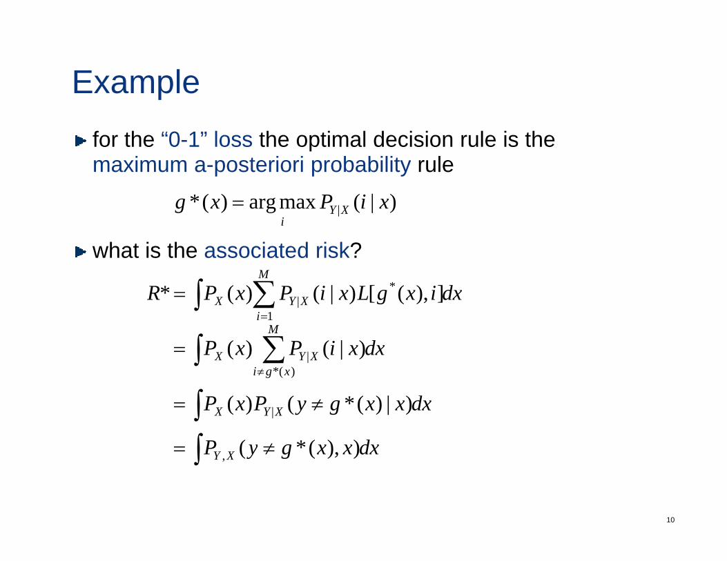
Examplefor the “0-1” loss the optimal decision rule is the maximum a-posteriori probability rulep p y
h t i th i t d i k?
)|(maxarg)(* | xiPxg XYi
=
what is the associated risk?
dxixgLxiPxPRM
iXYX∫ ∑
=
= ]),([)|()(* *
1|
i=1
dxxiPxPM
xgiXYX∫ ∑
≠
= )|()()*(
|
dxxxgyPxP XYX∫ ≠= )|)(*()( |
dxxxgyP XY∫ ≠= )),(*(
10
gyXY∫ )),((,
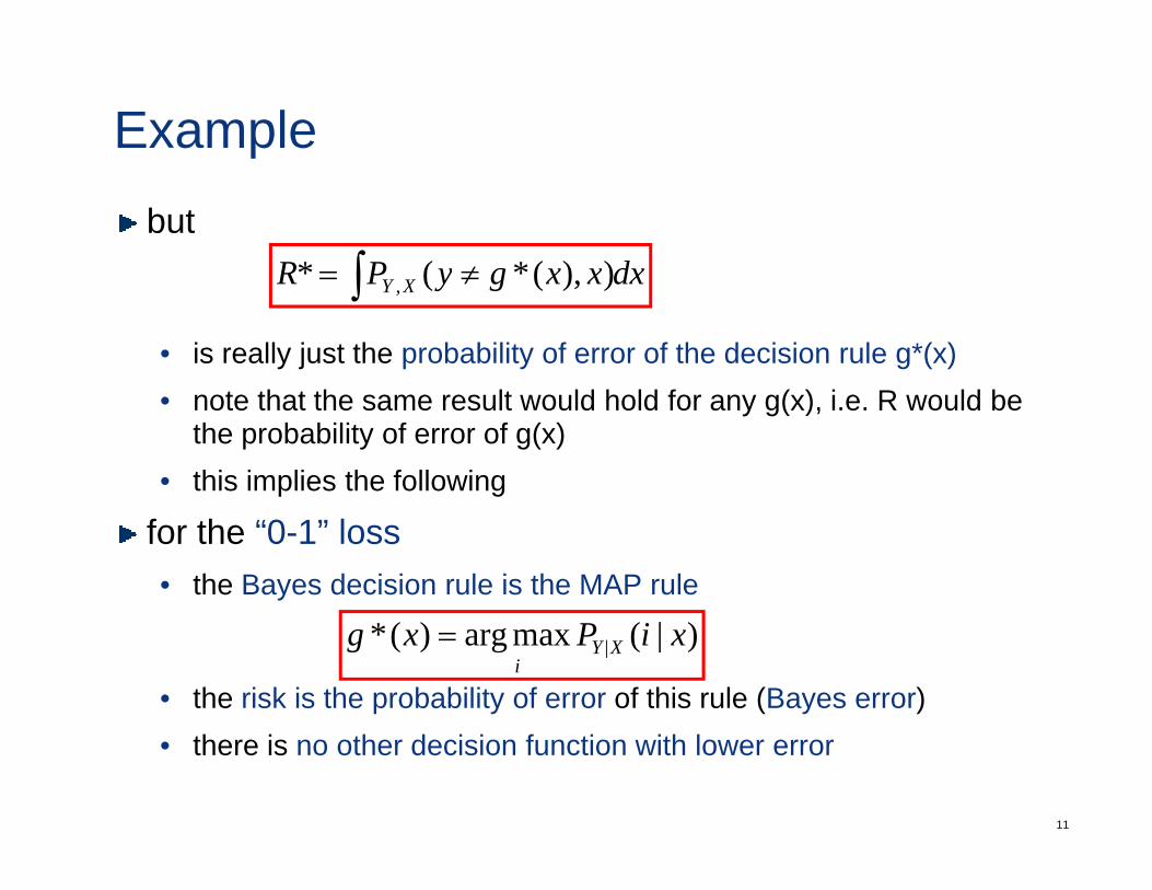
Examplebut
dxxxgyPR ∫ ≠= ))(*(*
• is really just the probability of error of the decision rule g*(x)f ( )
dxxxgyPR XY∫ ≠= )),((,
• note that the same result would hold for any g(x), i.e. R would be the probability of error of g(x)
• this implies the following
for the “0-1” loss• the Bayes decision rule is the MAP rule
• the risk is the probability of error of this rule (Bayes error)
)|(maxarg)(* | xiPxg XYi
=
11
• there is no other decision function with lower error
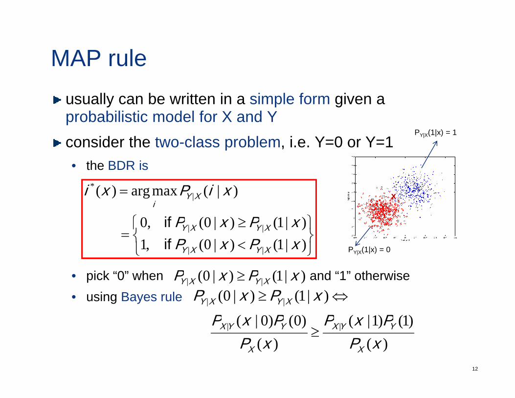
MAP ruleusually can be written in a simple form given a probabilistic model for X and Ypconsider the two-class problem, i.e. Y=0 or Y=1• the BDR is
PY|X(1|x) = 1
⎫⎧ ≥
=
)|1()|0(0
)|(maxarg)( |*
xPxP
xiPxi XYi
if
x
• pick “0” when and “1” otherwise
⎭⎬⎫
⎩⎨⎧
<≥
=)|1()|0(,1)|1()|0(,0
||
||
xPxPxPxP
XYXY
XYXY
if if
)|1()|0( xPxP ≥
PY|X(1|x) = 0
• pick 0 when and 1 otherwise• using Bayes rule
)|1()|0( || xPxP XYXY ≥
)1()1|()0()0|()|1()|0(
||
||
PxPPxPxPxP
YYXYYX
XYXY ⇔≥
12
)()1()1|(
)()0()0|( ||
xPPxP
xPPxP
X
YYX
X
YYX ≥
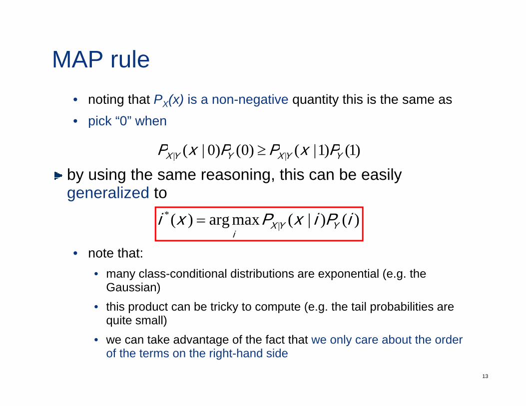
MAP rule• noting that PX(x) is a non-negative quantity this is the same as• pick “0” whenp
by using the same reasoning this can be easily)1()1|()0()0|( || YYXYYX PxPPxP ≥
by using the same reasoning, this can be easily generalized to
)()|(maxarg)( |* iPixPxi YYX=
• note that:• many class-conditional distributions are exponential (e.g. the
|i
y p ( gGaussian)
• this product can be tricky to compute (e.g. the tail probabilities are quite small)
13
• we can take advantage of the fact that we only care about the order of the terms on the right-hand side
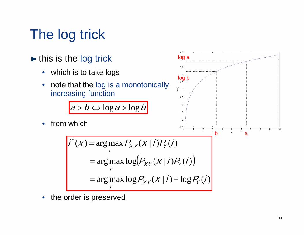
The log trickthis is the log trick• which is to take logs
log a
which is to take logs• note that the log is a monotonically
increasing function
log b
• from which
baba loglog >⇔>
ab ab
( ))()|(logmaxarg
)()|(maxarg)( |*
iPixP
iPixPxi YYXi
=
=
( ))(log)|(logmaxarg
)()|(logmaxarg
|
|
iPixP
iPixP
YYXi
YYXi
+=
=
14
• the order is preserved
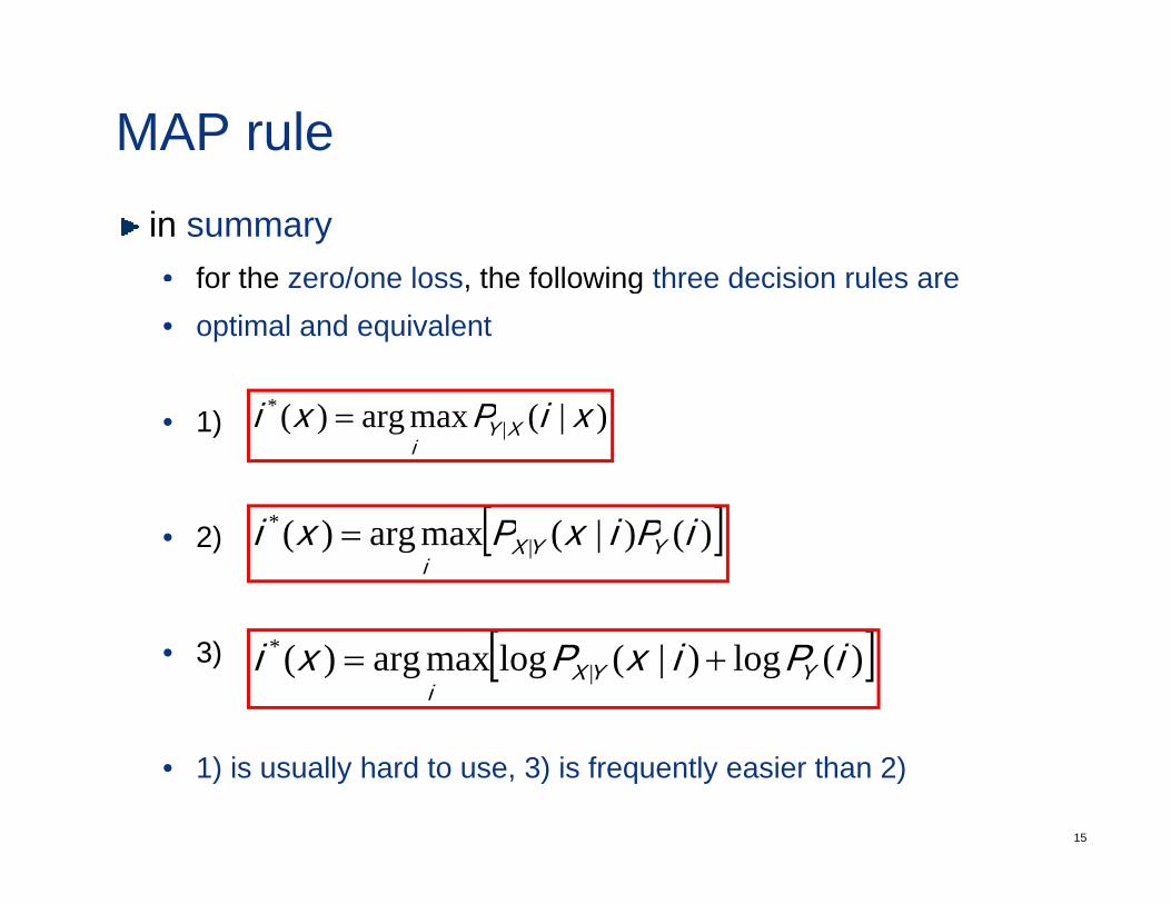
MAP rulein summary• for the zero/one loss the following three decision rules arefor the zero/one loss, the following three decision rules are• optimal and equivalent
• 1) )|(maxarg)( |* xiPxi XY
i=
[ ]• 2) [ ])()|(maxarg)( |* iPixPxi YYX
i=
• 3) [ ])(log)|(logmaxarg)( |* iPixPxi YYX
i+=
15
• 1) is usually hard to use, 3) is frequently easier than 2)
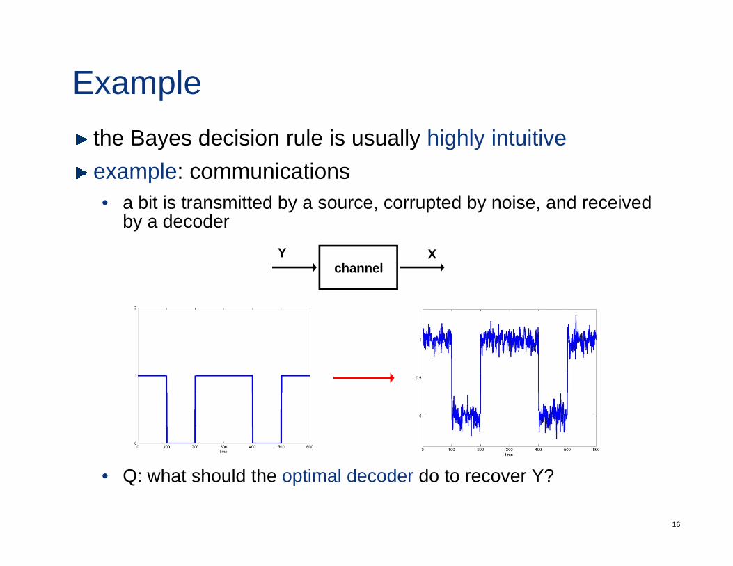
Examplethe Bayes decision rule is usually highly intuitiveexample: communicationsexample: communications• a bit is transmitted by a source, corrupted by noise, and received
by a decoder
channelY X
16
• Q: what should the optimal decoder do to recover Y?
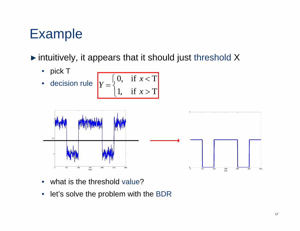
Exampleintuitively, it appears that it should just threshold X• pick Tpick T• decision rule
⎩⎨⎧
><
=T if,1T if,0
xx
Y
• what is the threshold value?
17
• let’s solve the problem with the BDR
Examplewe need• class probabilities:
• in the absence of any other info let’s say
21)1()0( == YY PP
• class-conditional densities:• noise results from thermal processes, electrons moving around and
b i h th
2
bumping each other• a lot of independent events that add up• by the central limit theorem it appears reasonable to assume that the
noise is Gaussian
we denote a Gaussian random variable of mean µ and variance σ2 by 2
18
σ y),(~ 2σµNX
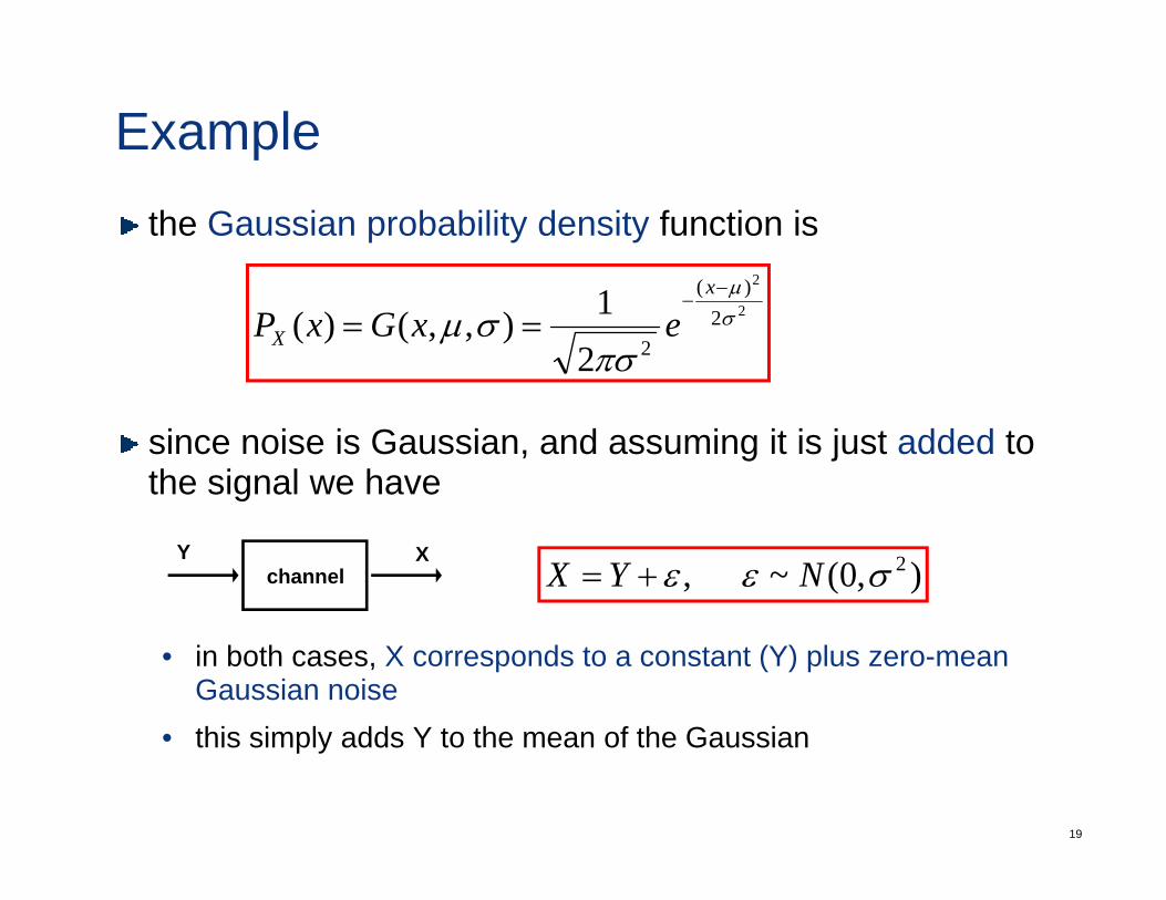
Examplethe Gaussian probability density function is
2)(2
2
2)(
221),,()( σ
µ
πσσµ
−−
==x
X exGxP
since noise is Gaussian, and assuming it is just added to the signal we have
channelY X
),0(~ , 2σεε NYX +=
• in both cases, X corresponds to a constant (Y) plus zero-mean Gaussian noise
• this simply adds Y to the mean of the Gaussian
19
• this simply adds Y to the mean of the Gaussian
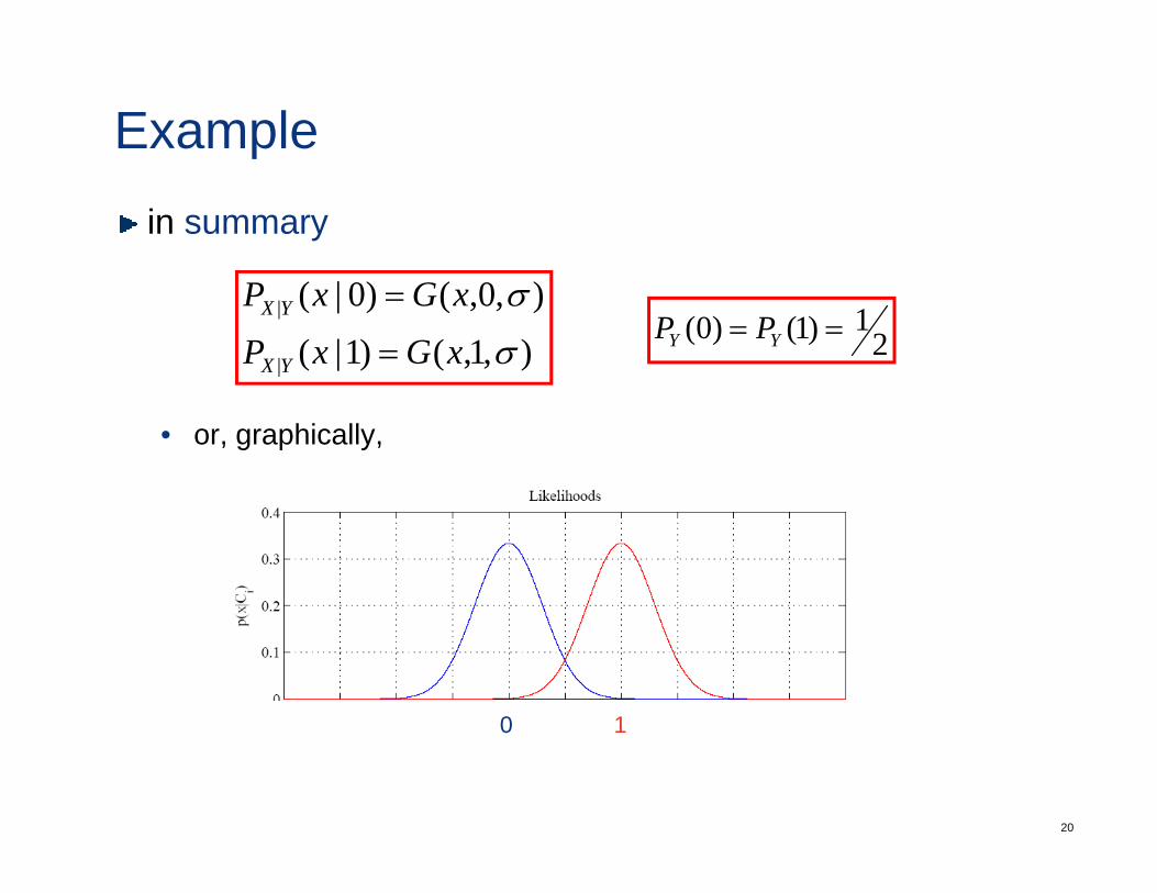
Examplein summary
),1,()1|(),0,()0|(
|
|
σ
σ
xGxPxGxP
YX
YX
=
=2
1)1()0( == YY PP
• or, graphically,
10
20
10
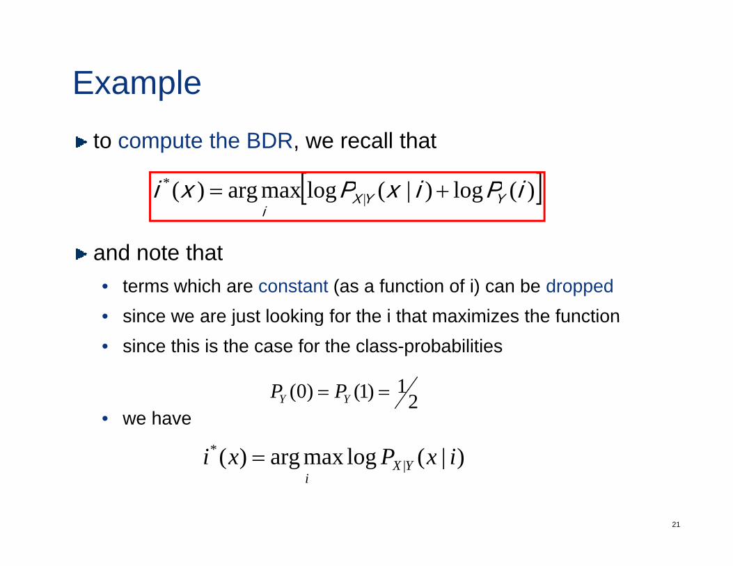
Exampleto compute the BDR, we recall that
[ ]
d t th t
[ ])(log)|(logmaxarg)( |* iPixPxi YYX
i+=
and note that • terms which are constant (as a function of i) can be dropped• since we are just looking for the i that maximizes the functionsince we are just looking for the i that maximizes the function• since this is the case for the class-probabilities
1)1()0( == PP• we have
21)1()0( == YY PP
)|(logmaxarg)( |* ixPxi YX=
21
)|(logmaxarg)( | ixPxi YXi
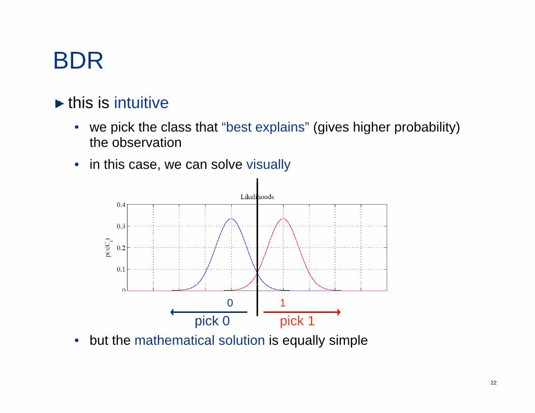
BDRthis is intuitive• we pick the class that “best explains” (gives higher probability)we pick the class that best explains (gives higher probability)
the observation• in this case, we can solve visually
b t th th ti l l ti i ll i l
10
pick 1pick 0
22
• but the mathematical solution is equally simple
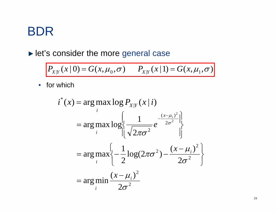
BDRlet’s consider the more general case
)()1|()()0|( GPGP
• for which
),,()1|( ),,()0|( 1|0| σµσµ xGxPxGxP YXYX ==
)|(logmaxarg)( |* ixPxi YX
i=
)(1 2
2µx i ⎪⎫⎪⎧−
−
2
22
)(1
21logmaxarg 2
µ
πσσ
i
x
e
⎫⎧
⎪⎭
⎪⎬
⎪⎩
⎪⎨=
2
22
)(
2)()2log(
21maxarg
µ
σµπσ i
i
x
x
⎭⎬⎫
⎩⎨⎧ −
−−=
23
22)(minarg
σµi
i
x −=
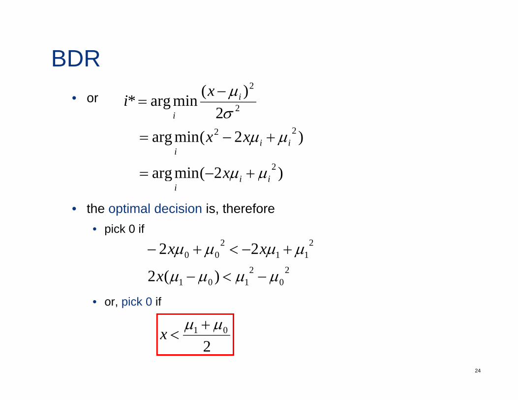
BDR• or
2)(minarg* 2
2i
i
xiσµ−
=
)2(minarg
)2(minarg
2
22ii
i
x
xx
µµ
µµ
+−=
+−=
• the optimal decision is, thereforei k 0 if
)2(minarg iii
x µµ +=
• pick 0 if
22
211
200
)(2
22
µµµµ
µµµµ
<
+−<+−
x
xx
• or, pick 0 if
0101 )(2 µµµµ −<−x
µµ +
24
201 µµ +
<x
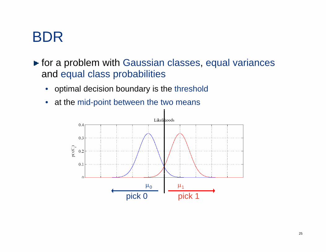
BDRfor a problem with Gaussian classes, equal variancesand equal class probabilitiesq p• optimal decision boundary is the threshold• at the mid-point between the two means
µ1µ0
pick 1pick 0
25
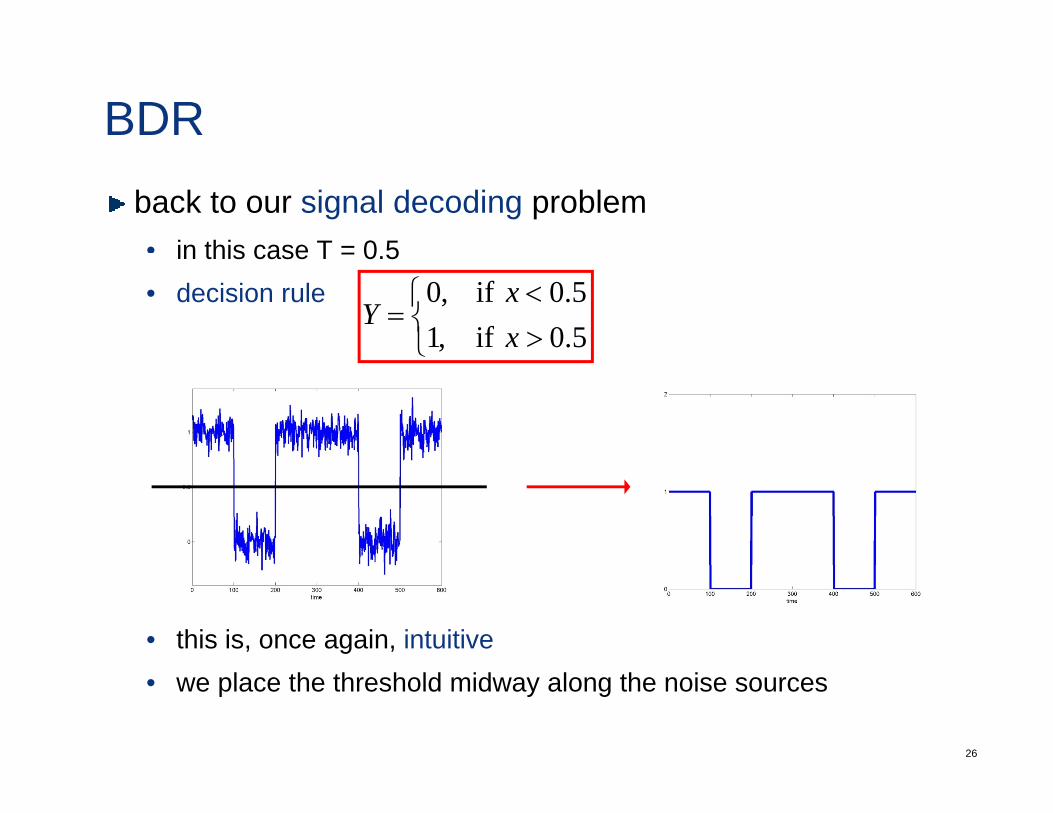
BDRback to our signal decoding problem• in this case T = 0 5in this case T = 0.5• decision rule
⎩⎨⎧
><
=5.0 if,15.0 if,0
xx
Y⎩
• this is, once again, intuitive
26
• we place the threshold midway along the noise sources
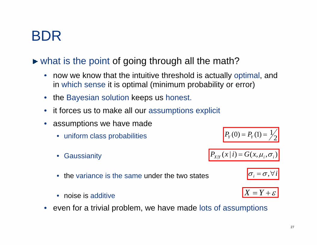
BDRwhat is the point of going through all the math?• now we know that the intuitive threshold is actually optimal andnow we know that the intuitive threshold is actually optimal, and
in which sense it is optimal (minimum probability or error)• the Bayesian solution keeps us honest.• it forces us to make all our assumptions explicit• assumptions we have made
• uniform class probabilities 21)1()0( == YY PPuniform class probabilities
• Gaussianity
2)()( YY
),,()|(| iiYX xGixP σµ=
• the variance is the same under the two states
• noise is additive ε+= YX
ii ∀= ,σσ
27
• even for a trivial problem, we have made lots of assumptions
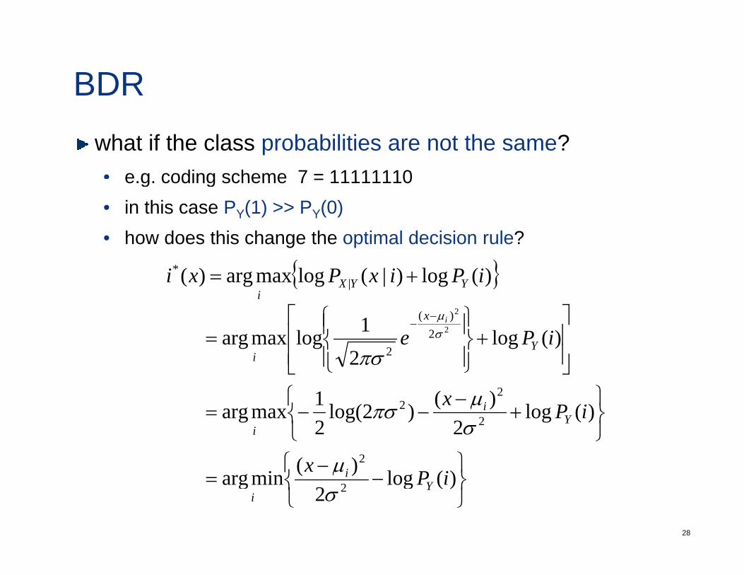
BDRwhat if the class probabilities are not the same?• e g coding scheme 7 = 11111110e.g. coding scheme 7 = 11111110• in this case PY(1) >> PY(0)• how does this change the optimal decision rule?
{ })(log)|(logmaxarg)( |* iPixPxi YYX
i+=
⎥⎤
⎢⎡ ⎪⎫⎪⎧
−−1 )( 2x iµ
⎫⎧
⎥⎥⎦
⎤
⎢⎢⎣
⎡+
⎪⎭
⎪⎬⎫
⎪⎩
⎪⎨⎧
=−
)(1
)(log2
1logmaxarg
2
22
2
x
iPe Yi
µ
πσσ
⎫⎧ −
⎭⎬⎫
⎩⎨⎧
+−
−−=
)(
)(log2
)()2log(21maxarg
2
22
x
iPxY
i
i
µ
σµπσ
28
⎭⎬⎫
⎩⎨⎧
−= )(log2
)(minarg 2 iPxY
i
i σµ
BDR• or )(log
2)(minarg* 2
2
iPxi Yi
i σµ
⎭⎬⎫
⎩⎨⎧
−−
=
))(log22(minarg
))(log22(minarg
22
222
iPx
iPxx Yiii
σµµ
σµµ
+=
−+−=
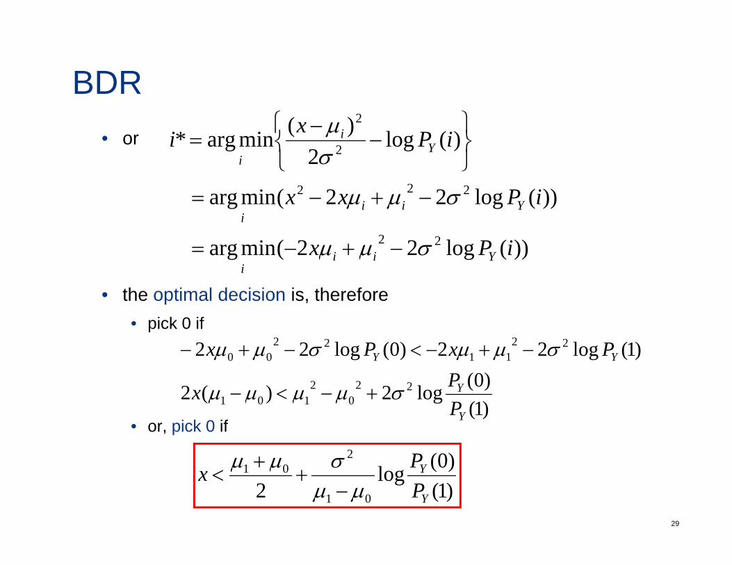
• the optimal decision is, thereforei k 0 if
))(log22(minarg iPx Yiii
σµµ −+−=
• pick 0 if
)0(l2)(2
)1(log22)0(log22
222
2211
2200
Y
YY
PPxPx σµµσµµ
+<
−+−<−+−
• or, pick 0 if)1()(log2)(2 2
0101Y
Y
Px σµµµµ +−<−
)0(2 Pσµµ +
29
)1()0(log
2 01
01
Y
Y
PPx
µµσµµ−
++
<
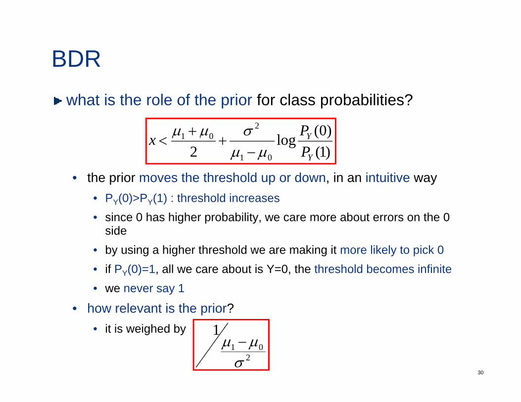
BDRwhat is the role of the prior for class probabilities?
)(2
the prior moves the threshold up or down in an intuitive way
)1()0(log
2 01
201
Y
Y
PPx
µµσµµ−
++
<
• the prior moves the threshold up or down, in an intuitive way• PY(0)>PY(1) : threshold increases• since 0 has higher probability, we care more about errors on the 0
idside• by using a higher threshold we are making it more likely to pick 0• if PY(0)=1, all we care about is Y=0, the threshold becomes infinite• we never say 1
• how relevant is the prior?• it is weighed by 1
30
• it is weighed by
201
1
σµµ −
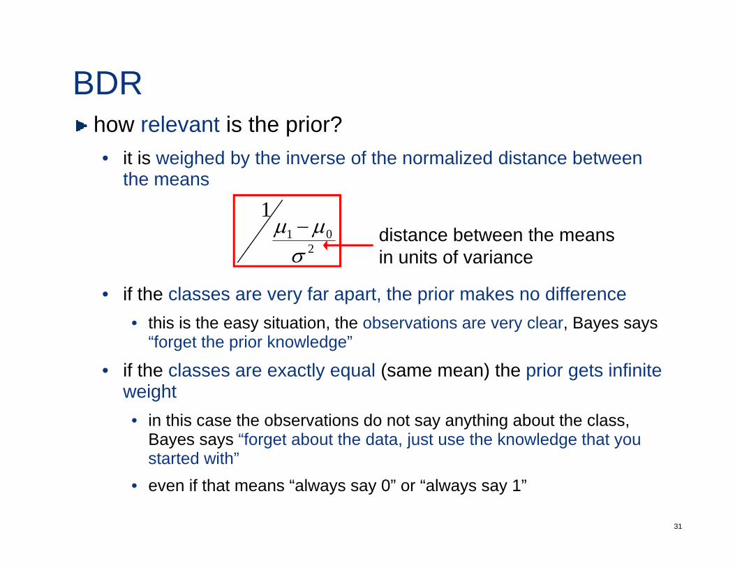
BDRhow relevant is the prior?• it is weighed by the inverse of the normalized distance between
the meansthe means
201
1µµ − distance between the means
• if the classes are very far apart, the prior makes no differencethis is the easy situation the observations are very clear Bayes says
2σ in units of variance
• this is the easy situation, the observations are very clear, Bayes says “forget the prior knowledge”
• if the classes are exactly equal (same mean) the prior gets infinite weightweight• in this case the observations do not say anything about the class,
Bayes says “forget about the data, just use the knowledge that you started with”
31
started with• even if that means “always say 0” or “always say 1”

32