bayesian decision theory - eecs.yorku.ca bayesian... · bayesian decision theory: topics 1....
TRANSCRIPT
J. Elder CSE 4404/5327 Introduction to Machine Learning and Pattern Recognition
Last updated: September 17, 2012
BAYESIAN DECISION THEORY
Probability & Bayesian Inference
J. Elder CSE 4404/5327 Introduction to Machine Learning and Pattern Recognition
2
Problems
¨ The following problems from the textbook are relevant: ¤ 2.1 – 2.9, 2.11, 2.17
¨ For this week, please at least solve Problem 2.3. We will go over this in class.

Probability & Bayesian Inference
J. Elder CSE 4404/5327 Introduction to Machine Learning and Pattern Recognition
3
Credits
¨ Some of these slides were sourced and/or modified from: ¤ Christopher Bishop, Microsoft UK ¤ Simon Prince, University College London ¤ Sergios Theodoridis, University of Athens & Konstantinos
Koutroumbas, National Observatory of Athens
Probability & Bayesian Inference
J. Elder CSE 4404/5327 Introduction to Machine Learning and Pattern Recognition
4
Bayesian Decision Theory: Topics
1. Probability 2. The Univariate Normal Distribution 3. Bayesian Classifiers 4. Minimizing Risk 5. Nonparametric Density Estimation 6. Training and Evaluation Methods
Probability & Bayesian Inference
J. Elder CSE 4404/5327 Introduction to Machine Learning and Pattern Recognition
5
Bayesian Decision Theory: Topics
1. Probability 2. The Univariate Normal Distribution 3. Bayesian Classifiers 4. Minimizing Risk 5. Nonparametric Density Estimation 6. Training and Evaluation Methods
Probability & Bayesian Inference
J. Elder CSE 4404/5327 Introduction to Machine Learning and Pattern Recognition
6
Probability
¨ “Probability theory is nothing but common sense reduced to calculation”
- Pierre Laplace, 1812.
Probability & Bayesian Inference
J. Elder CSE 4404/5327 Introduction to Machine Learning and Pattern Recognition
7
Random Variables
¨ A random variable is a variable whose value is uncertain.
¨ For example, the height of a randomly selected person in this class is a random variable – I won’t know its value until the person is selected.
¨ Note that we are not completely uncertain about most random variables. ¤ For example, we know that height will probably be in the 5’-6’ range.
¤ In addition, 5’6” is more likely than 5’0” or 6’0”.
¨ The function that describes the probability of each possible value of the random variable is called a probability distribution.
Probability & Bayesian Inference
J. Elder CSE 4404/5327 Introduction to Machine Learning and Pattern Recognition
8
Probability Distributions
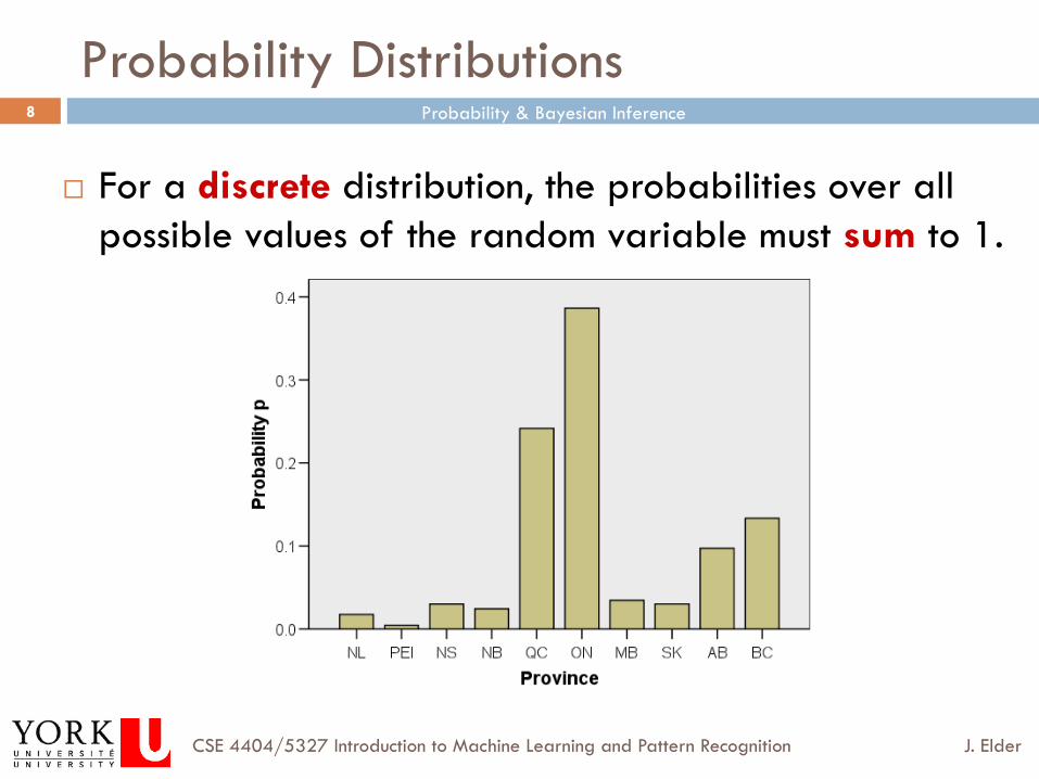
¨ For a discrete distribution, the probabilities over all possible values of the random variable must sum to 1.
Probability & Bayesian Inference
J. Elder CSE 4404/5327 Introduction to Machine Learning and Pattern Recognition
9
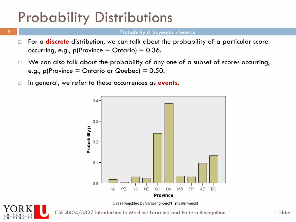
Probability Distributions ¨ For a discrete distribution, we can talk about the probability of a particular score
occurring, e.g., p(Province = Ontario) = 0.36.
¨ We can also talk about the probability of any one of a subset of scores occurring, e.g., p(Province = Ontario or Quebec) = 0.50.
¨ In general, we refer to these occurrences as events.
Probability & Bayesian Inference
J. Elder CSE 4404/5327 Introduction to Machine Learning and Pattern Recognition
10
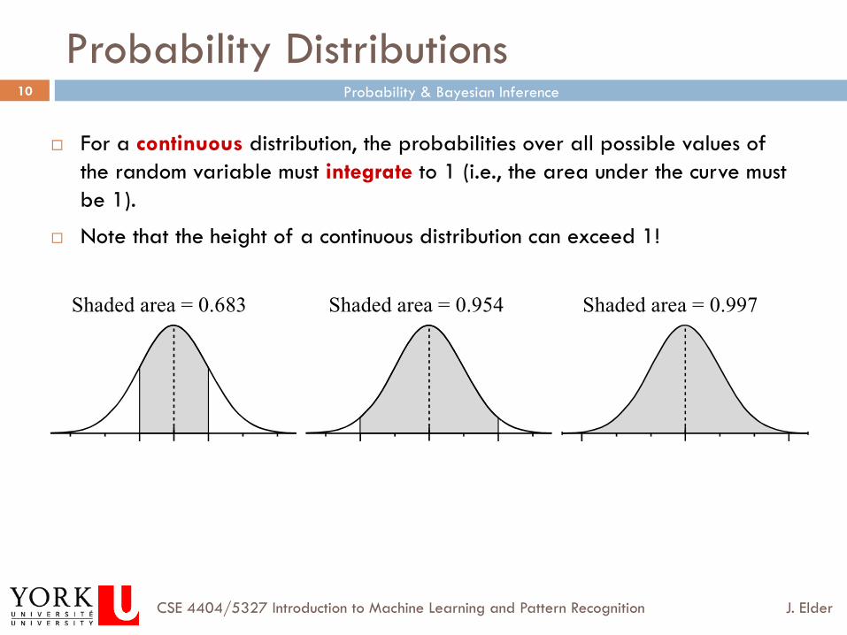
Probability Distributions
¨ For a continuous distribution, the probabilities over all possible values of the random variable must integrate to 1 (i.e., the area under the curve must be 1).
¨ Note that the height of a continuous distribution can exceed 1!
S h a d e d a r e a = 0 . 6 8 3 S h a d e d a r e a = 0 . 9 5 4 S h a d e d a r e a = 0 . 9 9 7
Probability & Bayesian Inference
J. Elder CSE 4404/5327 Introduction to Machine Learning and Pattern Recognition
11
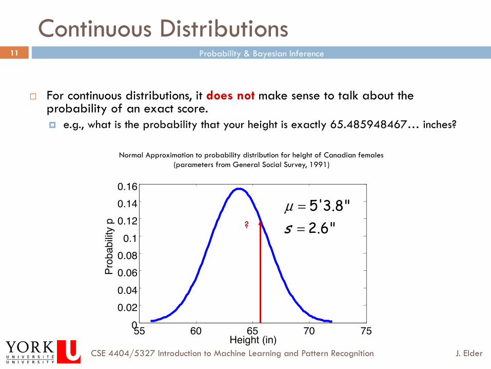
Continuous Distributions
¨ For continuous distributions, it does not make sense to talk about the probability of an exact score. ¤ e.g., what is the probability that your height is exactly 65.485948467… inches?
55 60 65 70 75 0 0.02 0.04 0.06 0.08
0.1 0.12 0.14 0.16
Height (in)
Prob
abilit
y p
Normal Approximation to probability distribution for height of Canadian females (parameters from General Social Survey, 1991)
5'3.8"2.6"s
µ ==?
Probability & Bayesian Inference
J. Elder CSE 4404/5327 Introduction to Machine Learning and Pattern Recognition
12
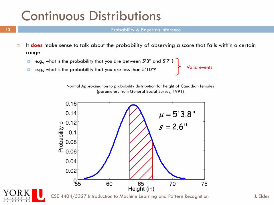
Continuous Distributions
¨ It does make sense to talk about the probability of observing a score that falls within a certain range ¤ e.g., what is the probability that you are between 5’3” and 5’7”?
¤ e.g., what is the probability that you are less than 5’10”?
55 60 65 70 75 0 0.02 0.04 0.06 0.08
0.1 0.12 0.14 0.16
Height (in)
Prob
abilit
y p
Normal Approximation to probability distribution for height of Canadian females (parameters from General Social Survey, 1991)
5'3.8"2.6"s
µ ==
Valid events
Probability & Bayesian Inference
J. Elder CSE 4404/5327 Introduction to Machine Learning and Pattern Recognition
13
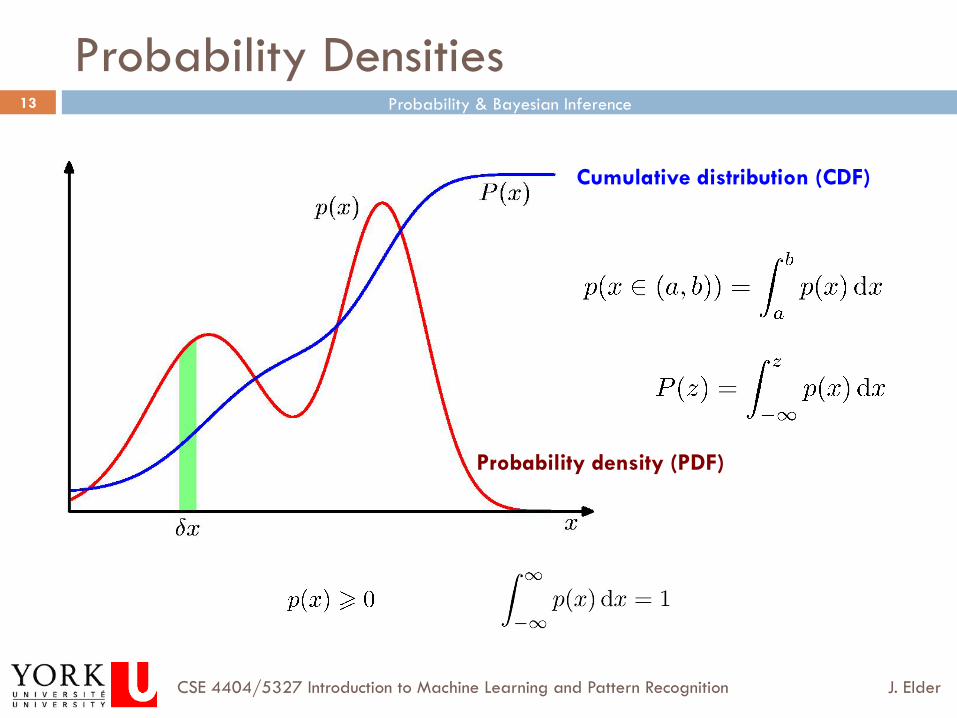
Probability Densities
Probability density (PDF)
Cumulative distribution (CDF)
Probability & Bayesian Inference
J. Elder CSE 4404/5327 Introduction to Machine Learning and Pattern Recognition
14
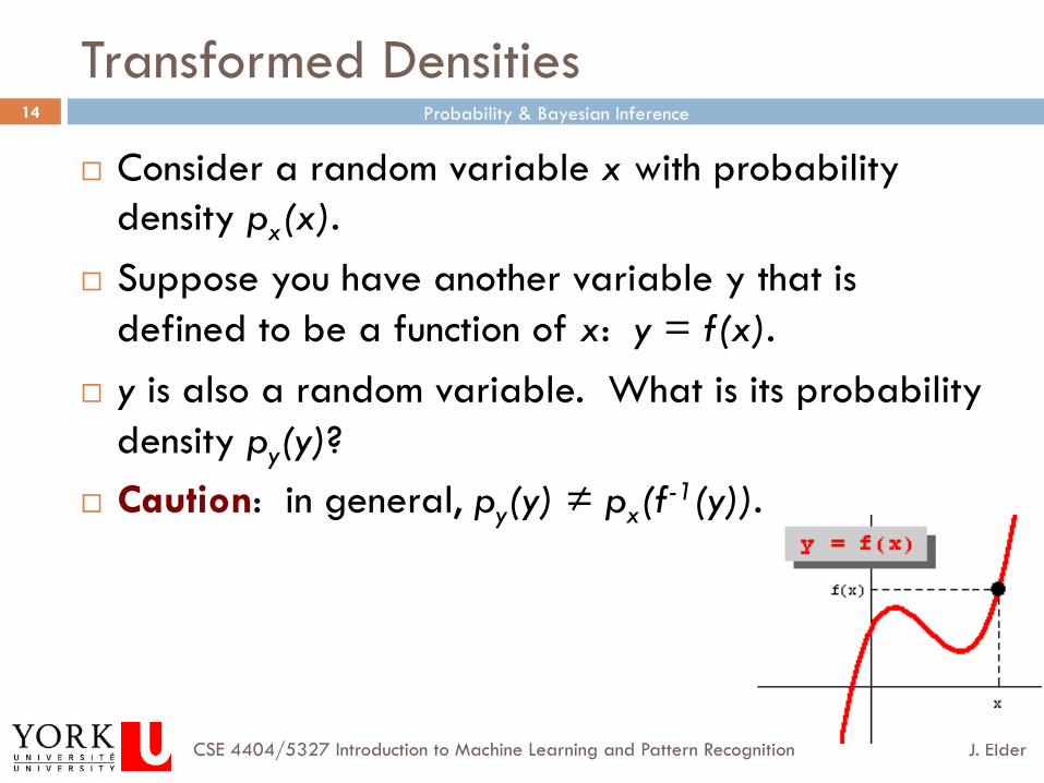
Transformed Densities
¨ Consider a random variable x with probability density px(x).
¨ Suppose you have another variable y that is defined to be a function of x: y = f(x).
¨ y is also a random variable. What is its probability density py(y)?
¨ Caution: in general, py(y) ≠ px(f-1(y)).
Probability & Bayesian Inference
J. Elder CSE 4404/5327 Introduction to Machine Learning and Pattern Recognition
15
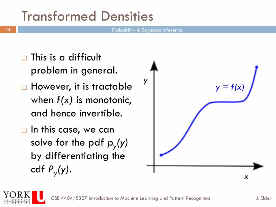
Transformed Densities
¨ This is a difficult problem in general.
¨ However, it is tractable when f(x) is monotonic, and hence invertible.
¨ In this case, we can solve for the pdf py(y) by differentiating the cdf Py(y).
y
x
y = f(x)
Probability & Bayesian Inference
J. Elder CSE 4404/5327 Introduction to Machine Learning and Pattern Recognition
16
Transformed Densities
¨ Let’s assume that y is monotonically increasing in x. Then we can write
¨ Taking derivatives, we get
Py (y) = P f (x) ≤ y( ) = P x ≤ f −1(y)( ) = Px f −1(y)( )
py (y) ddy
Py (y) = ddy
Px f −1(y)( ) = dxdy
ddx
Px x( ) = dxdy
px x( )where x = f −1(y).
Note that dxdy
> 0 in this case.
Probability & Bayesian Inference
J. Elder CSE 4404/5327 Introduction to Machine Learning and Pattern Recognition
17
Transformed Densities
¨ If y is monotonically decreasing in x, using the same method it is easy to show that
¨ Thus a general expression that applies when y is monotonic on x is:
py (y) = − dxdy
px x( )where x = f −1(y).
Note that dxdy
< 0 in this case.
py (y) = dxdy
px x( ),where x = f −1(y).
Probability & Bayesian Inference
J. Elder CSE 4404/5327 Introduction to Machine Learning and Pattern Recognition
18
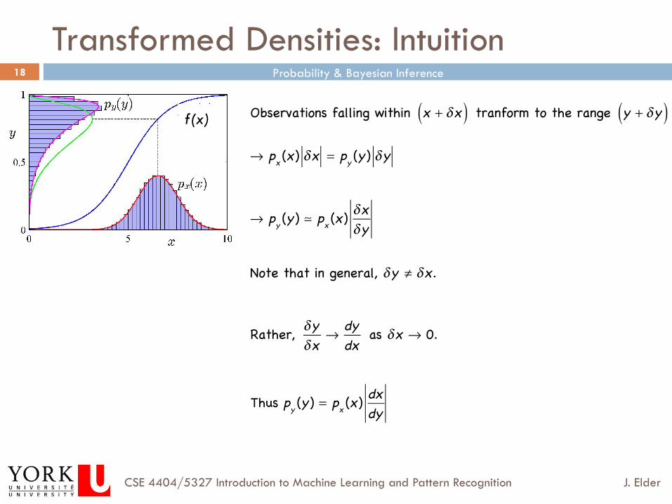
Transformed Densities: Intuition
Observations falling within x + δx( ) tranform to the range y + δy( )
→ px (x) δx = py (y ) δy
→ py (y ) px (x) δx
δy
Note that in general, δy ≠ δx.
Rather, δy
δx → dydx as δx → 0.
Thus py (y ) = px (x) dx
dy
f(x)
Probability & Bayesian Inference
J. Elder CSE 4404/5327 Introduction to Machine Learning and Pattern Recognition
19
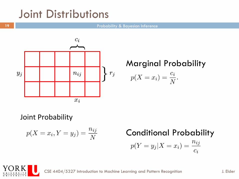
Joint Distributions
Marginal Probability
Conditional Probability
Joint Probability

Probability & Bayesian Inference
J. Elder CSE 4404/5327 Introduction to Machine Learning and Pattern Recognition
20
Joint Distributions
Sum Rule
Product Rule
Probability & Bayesian Inference
J. Elder CSE 4404/5327 Introduction to Machine Learning and Pattern Recognition
21
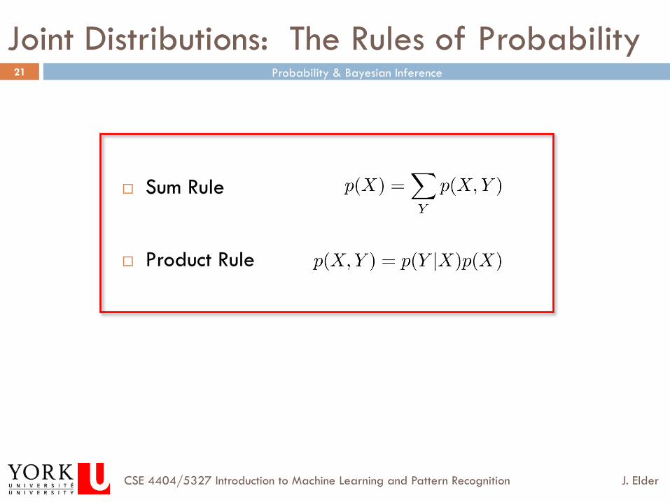
Joint Distributions: The Rules of Probability
¨ Sum Rule
¨ Product Rule
Probability & Bayesian Inference
J. Elder CSE 4404/5327 Introduction to Machine Learning and Pattern Recognition
22
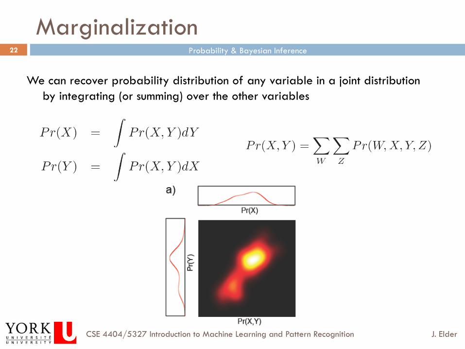
Marginalization
We can recover probability distribution of any variable in a joint distribution by integrating (or summing) over the other variables
Probability & Bayesian Inference
J. Elder CSE 4404/5327 Introduction to Machine Learning and Pattern Recognition
23
Conditional Probability
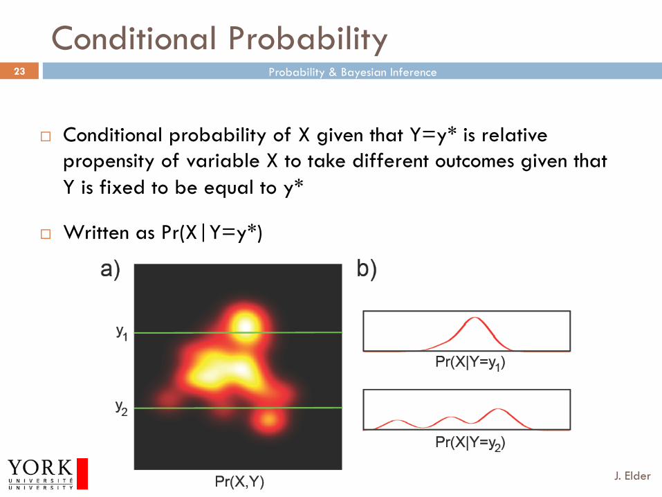
¨ Conditional probability of X given that Y=y* is relative propensity of variable X to take different outcomes given that Y is fixed to be equal to y*
¨ Written as Pr(X|Y=y*)
Probability & Bayesian Inference
J. Elder CSE 4404/5327 Introduction to Machine Learning and Pattern Recognition
24
Conditional Probability
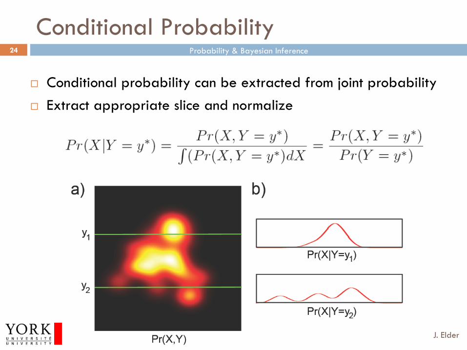
¨ Conditional probability can be extracted from joint probability ¨ Extract appropriate slice and normalize
Probability & Bayesian Inference
J. Elder CSE 4404/5327 Introduction to Machine Learning and Pattern Recognition
25
Conditional Probability
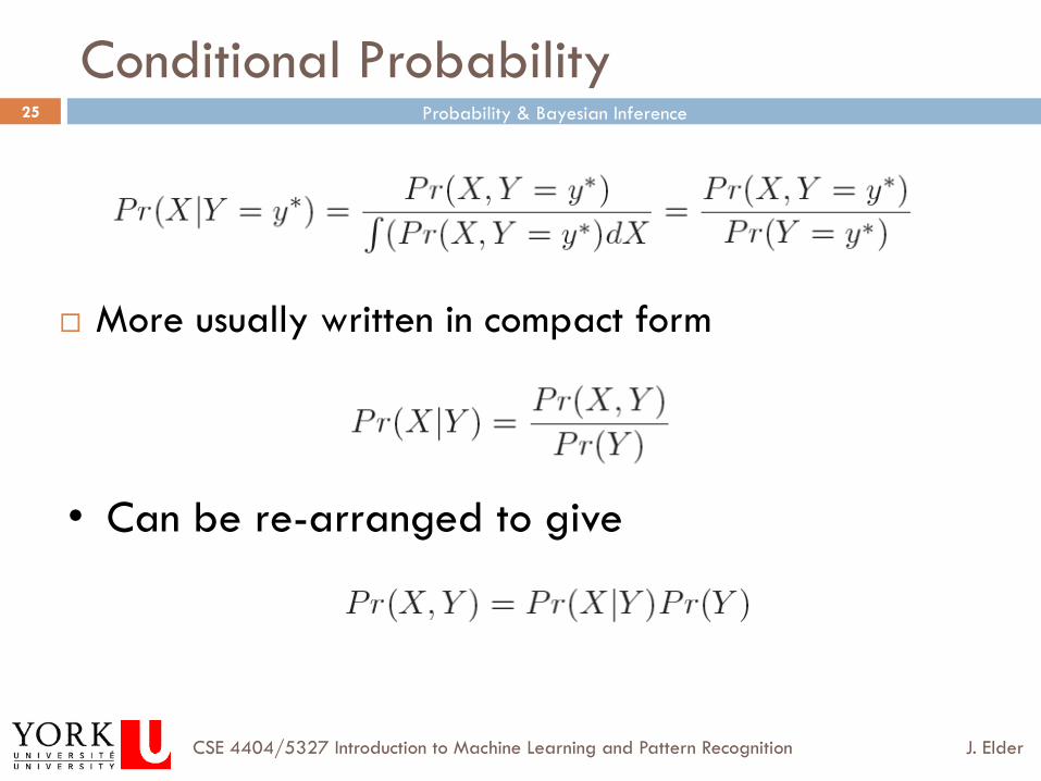
¨ More usually written in compact form
• Can be re-arranged to give

Probability & Bayesian Inference
J. Elder CSE 4404/5327 Introduction to Machine Learning and Pattern Recognition
26
Independence
¨ If two variables X and Y are independent then variable X tells us nothing about variable Y (and vice-versa)
Probability & Bayesian Inference
J. Elder CSE 4404/5327 Introduction to Machine Learning and Pattern Recognition
27
Independence
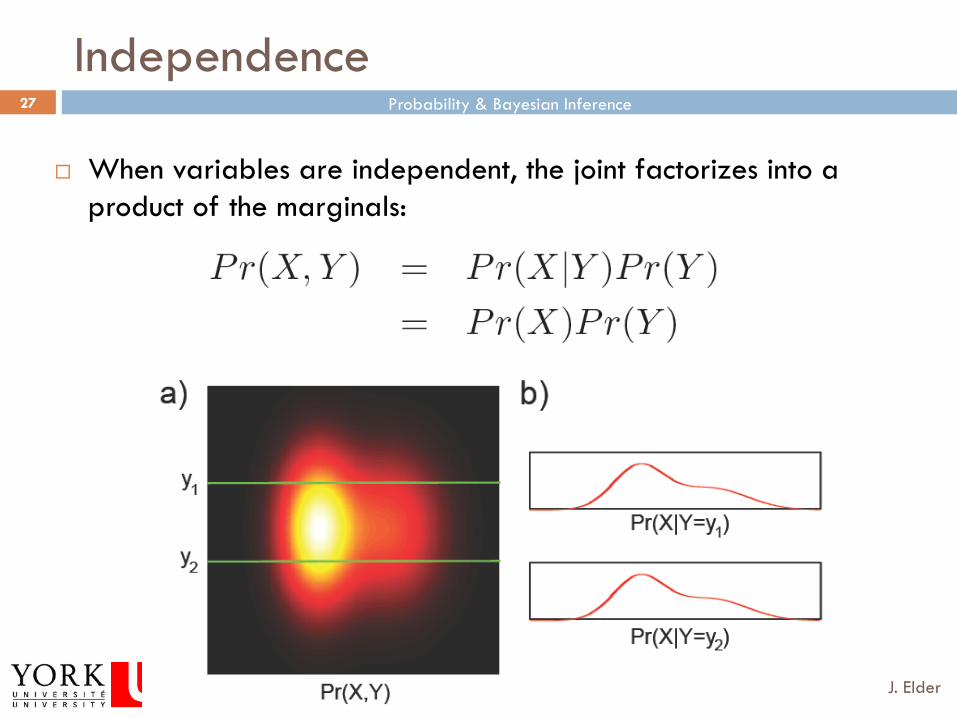
¨ When variables are independent, the joint factorizes into a product of the marginals:
Probability & Bayesian Inference
J. Elder CSE 4404/5327 Introduction to Machine Learning and Pattern Recognition
28
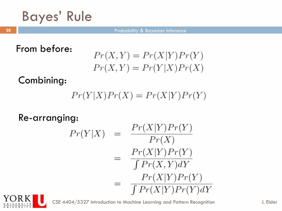
Bayes’ Rule
From before:
Combining:
Re-arranging:
Probability & Bayesian Inference
J. Elder CSE 4404/5327 Introduction to Machine Learning and Pattern Recognition
29
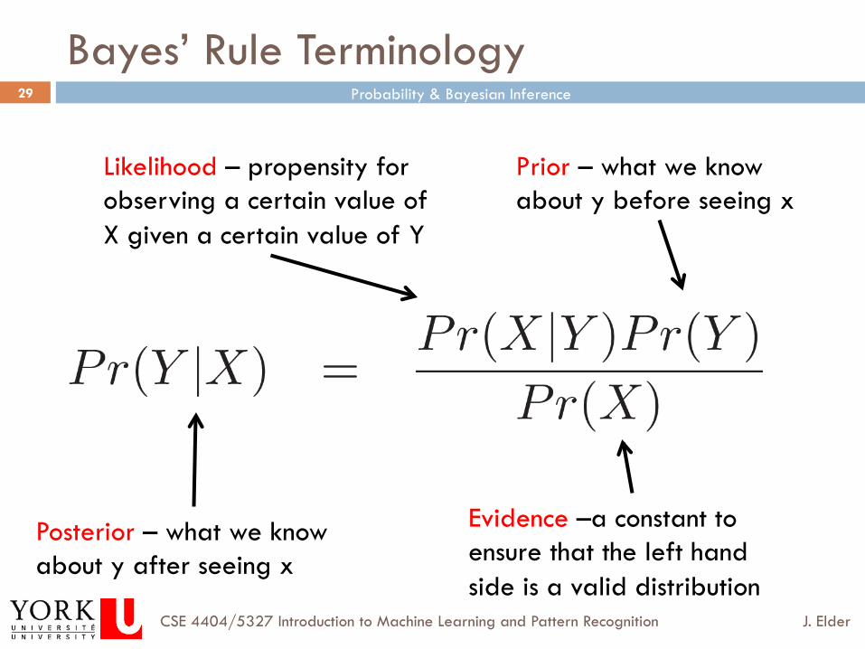
Bayes’ Rule Terminology
Posterior – what we know about y after seeing x
Prior – what we know about y before seeing x
Likelihood – propensity for observing a certain value of X given a certain value of Y
Evidence –a constant to ensure that the left hand side is a valid distribution
Probability & Bayesian Inference
J. Elder CSE 4404/5327 Introduction to Machine Learning and Pattern Recognition
30
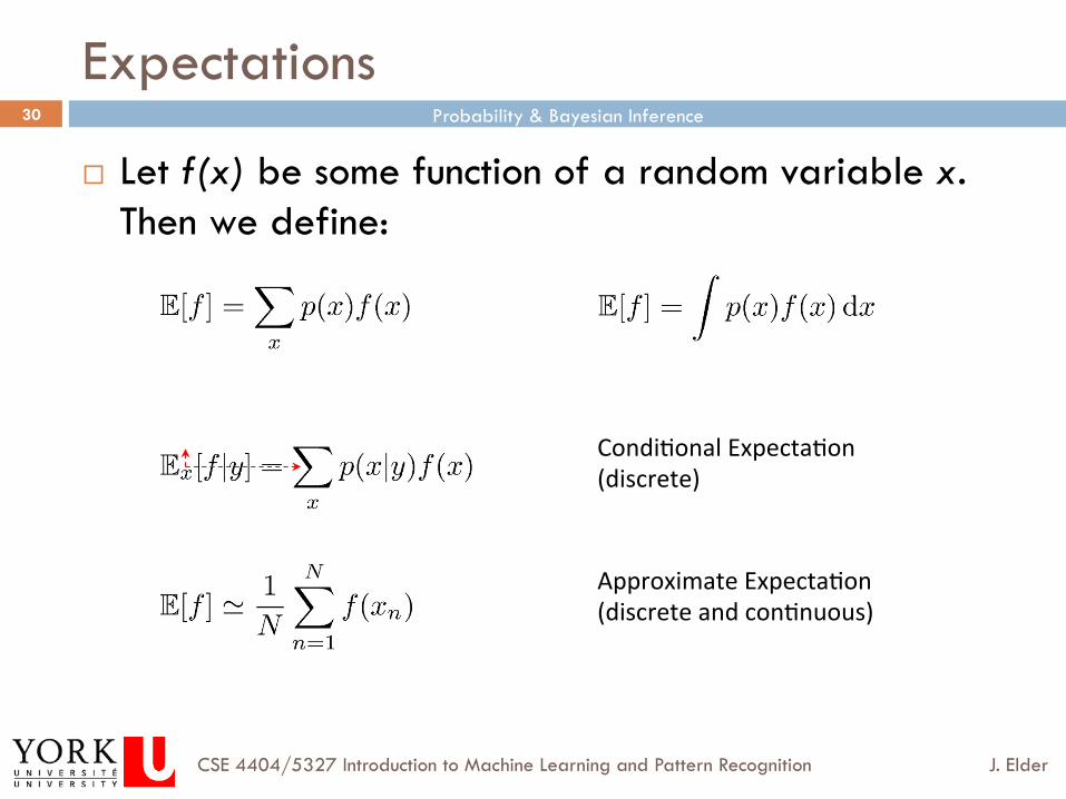
Expectations
¨ Let f(x) be some function of a random variable x. Then we define:
Condi3onal Expecta3on (discrete)
Approximate Expecta3on (discrete and con3nuous)
Probability & Bayesian Inference
J. Elder CSE 4404/5327 Introduction to Machine Learning and Pattern Recognition
31
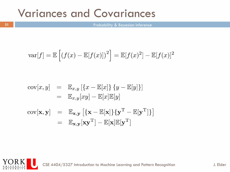
Variances and Covariances

Sept 10, 2012
End of Lecture
Probability & Bayesian Inference
J. Elder CSE 4404/5327 Introduction to Machine Learning and Pattern Recognition
33
Bayesian Decision Theory: Topics
1. Probability 2. The Univariate Normal Distribution
3. Bayesian Classifiers 4. Minimizing Risk 5. Nonparametric Density Estimation 6. Training and Evaluation Methods
Probability & Bayesian Inference
J. Elder CSE 4404/5327 Introduction to Machine Learning and Pattern Recognition
34
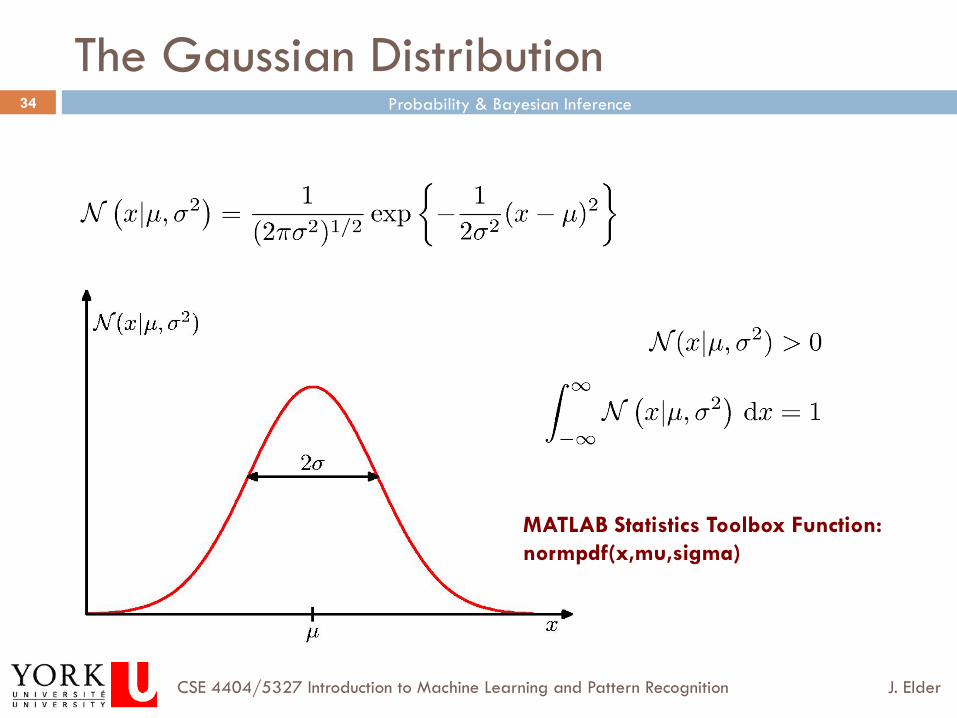
The Gaussian Distribution
MATLAB Statistics Toolbox Function: normpdf(x,mu,sigma)
Probability & Bayesian Inference
J. Elder CSE 4404/5327 Introduction to Machine Learning and Pattern Recognition
35
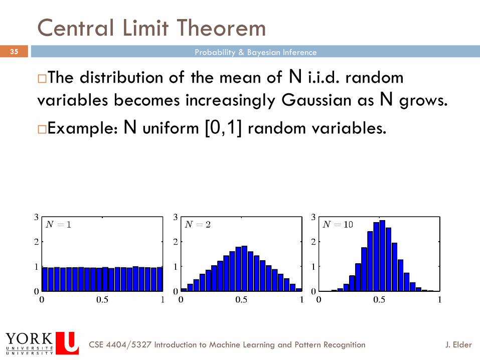
Central Limit Theorem
¨ The distribution of the mean of N i.i.d. random variables becomes increasingly Gaussian as N grows. ¨ Example: N uniform [0,1] random variables.
Probability & Bayesian Inference
J. Elder CSE 4404/5327 Introduction to Machine Learning and Pattern Recognition
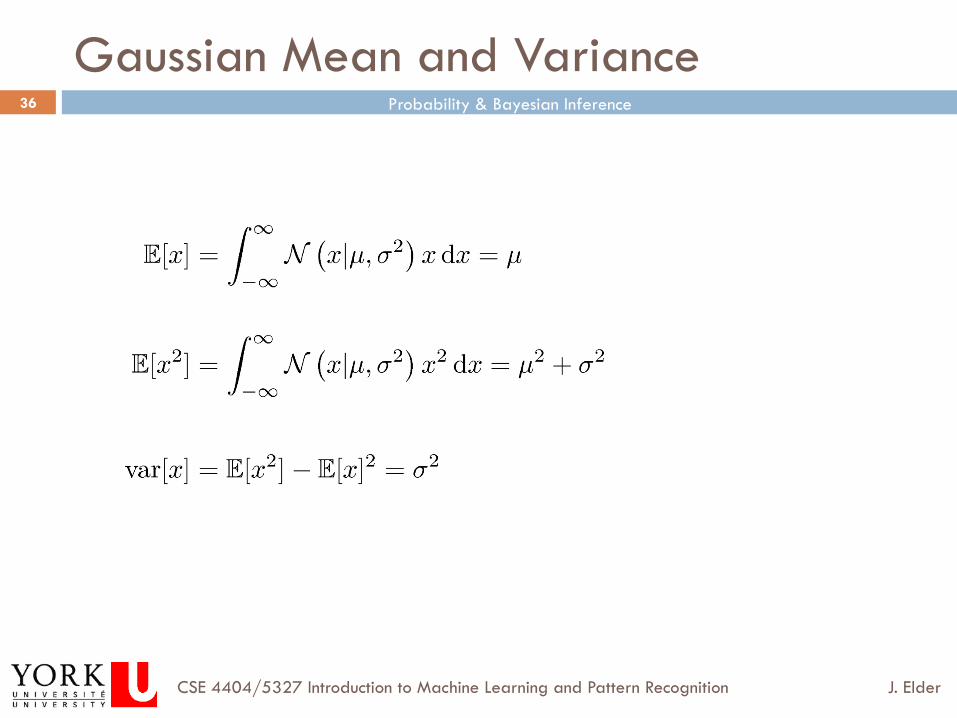
36
Gaussian Mean and Variance
Probability & Bayesian Inference
J. Elder CSE 4404/5327 Introduction to Machine Learning and Pattern Recognition
37
Bayesian Decision Theory: Topics
1. Probability 2. The Univariate Normal Distribution 3. Bayesian Classifiers
4. Minimizing Risk 5. Nonparametric Density Estimation 6. Training and Evaluation Methods
Probability & Bayesian Inference
J. Elder CSE 4404/5327 Introduction to Machine Learning and Pattern Recognition
38
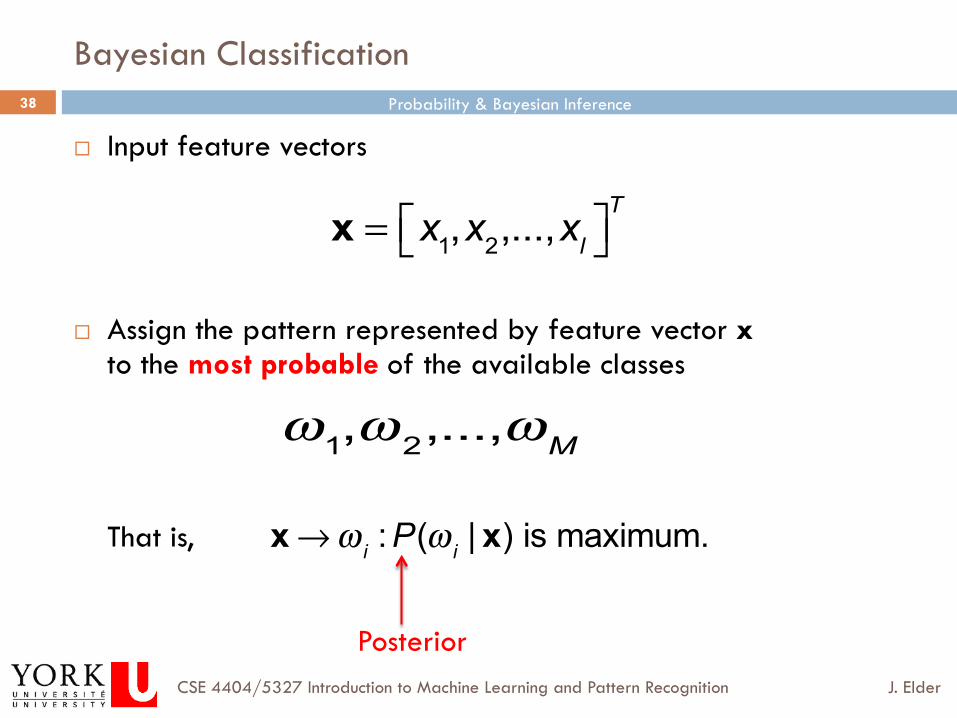
Bayesian Classification
¨ Input feature vectors
¨ Assign the pattern represented by feature vector x to the most probable of the available classes That is,
x = x1,x2,...,xl
⎡⎣ ⎤⎦T
ω1,ω 2,...,ωM
x →ω i :P(ω i | x) is maximum.
Posterior
Probability & Bayesian Inference
J. Elder CSE 4404/5327 Introduction to Machine Learning and Pattern Recognition
39
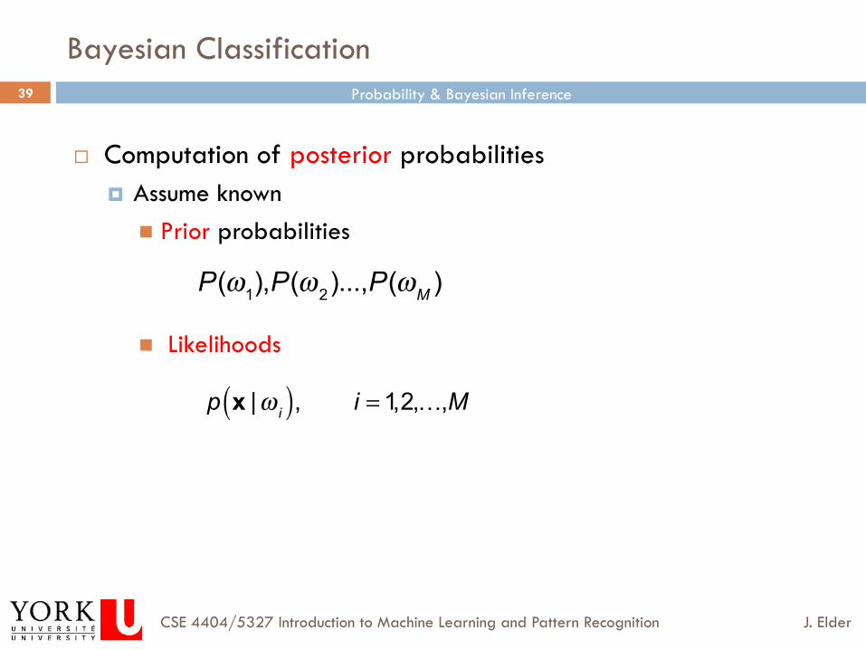
¨ Computation of posterior probabilities ¤ Assume known
n Prior probabilities
n Likelihoods
P(ω1),P(ω 2)...,P(ωM )
p x |ω i( ), i = 1,2,…,M
Bayesian Classification
Probability & Bayesian Inference
J. Elder CSE 4404/5327 Introduction to Machine Learning and Pattern Recognition
40
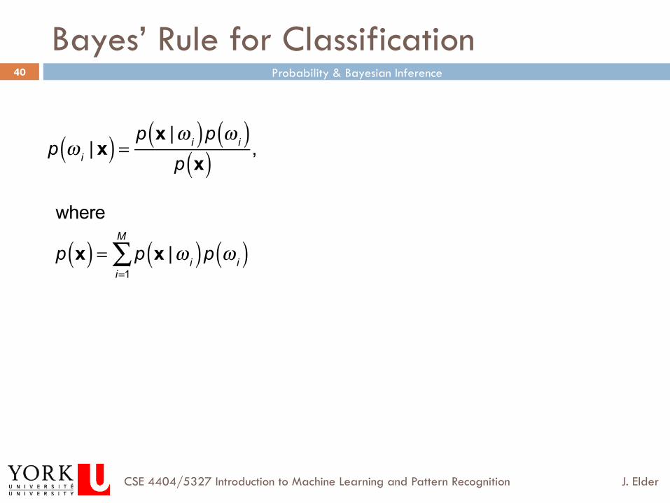
Bayes’ Rule for Classification
p ω i | x( ) = p x |ω i( )p ω i( )
p x( ) ,
where
p x( ) = p x |ω i( )p ω i( )i=1
M
∑
Probability & Bayesian Inference
J. Elder CSE 4404/5327 Introduction to Machine Learning and Pattern Recognition
41
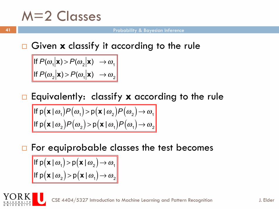
M=2 Classes
41 ¨ Given x classify it according to the rule
¨ Equivalently: classify x according to the rule
¨ For equiprobable classes the test becomes
If P(ω1 x) > P(ω 2 x) →ω1
If P(ω 2 x) > P(ω1 x) →ω 2
If p x |ω1( )P ω1( ) > p x |ω 2( )P ω 2( )→ω1
If p x |ω 2( )P ω 2( ) > p x |ω1( )P ω1( )→ω 2
If p x |ω1( ) > p x |ω 2( )→ω1
If p x |ω 2( ) > p x |ω1( )→ω 2
Probability & Bayesian Inference
J. Elder CSE 4404/5327 Introduction to Machine Learning and Pattern Recognition
42
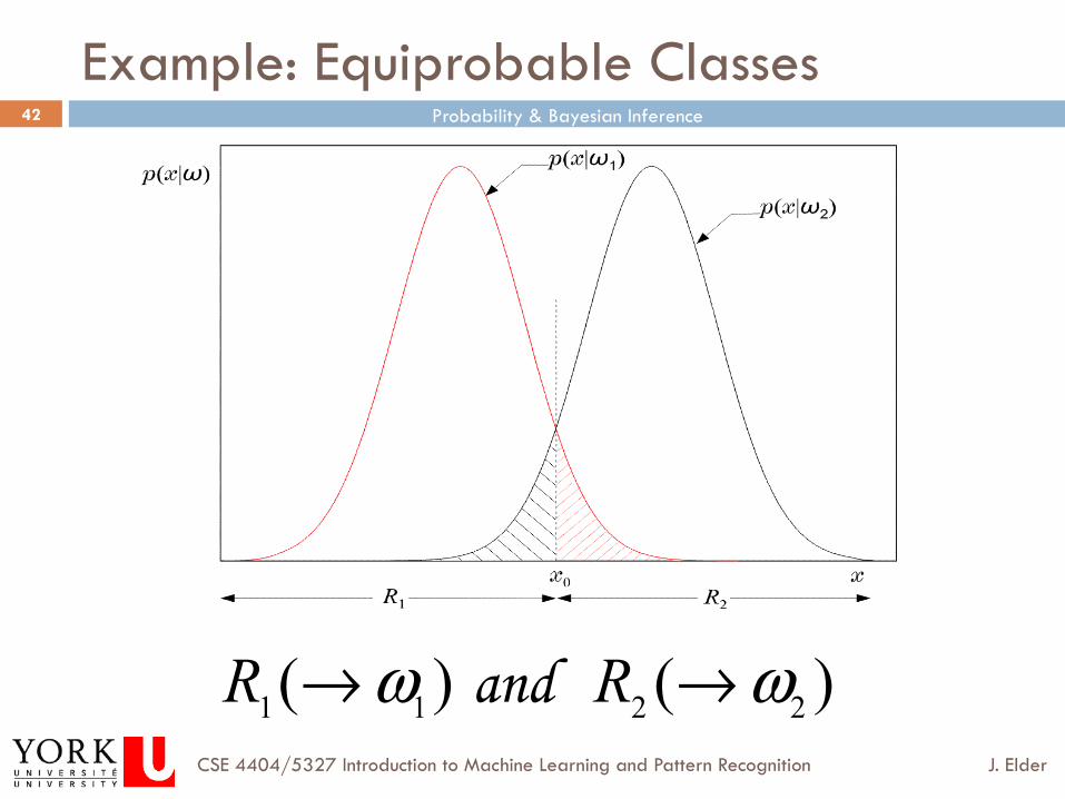
Example: Equiprobable Classes
)()( 2211 ωω →→ RR and
Probability & Bayesian Inference
J. Elder CSE 4404/5327 Introduction to Machine Learning and Pattern Recognition
43
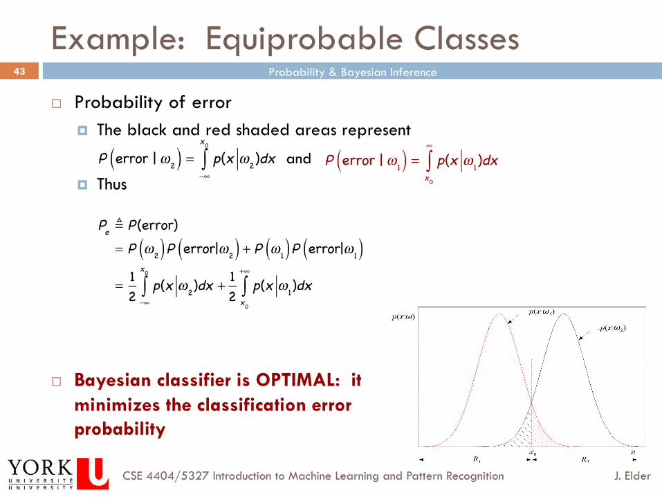
Example: Equiprobable Classes
43 ¨ Probability of error ¤ The black and red shaded areas represent
¤ Thus
¨ Bayesian classifier is OPTIMAL: it minimizes the classification error probability
Pe P(error)= P ω2( )P error|ω2( ) + P ω 1( )P error|ω 1( )= 1
2 p(x ω2 )dx +−∞
x0
∫12 p(x ω 1 )dx
x0
+∞
∫
P error | ω2( ) = p(x ω2 )dx
−∞
x0
∫ P error | ω 1( ) = p(x ω 1 )dx
x0
∞
∫and
Probability & Bayesian Inference
J. Elder CSE 4404/5327 Introduction to Machine Learning and Pattern Recognition
44
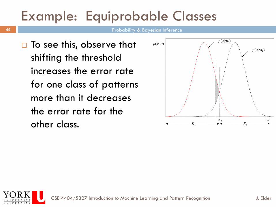
Example: Equiprobable Classes
¨ To see this, observe that shifting the threshold increases the error rate for one class of patterns more than it decreases the error rate for the other class.
Probability & Bayesian Inference
J. Elder CSE 4404/5327 Introduction to Machine Learning and Pattern Recognition
45
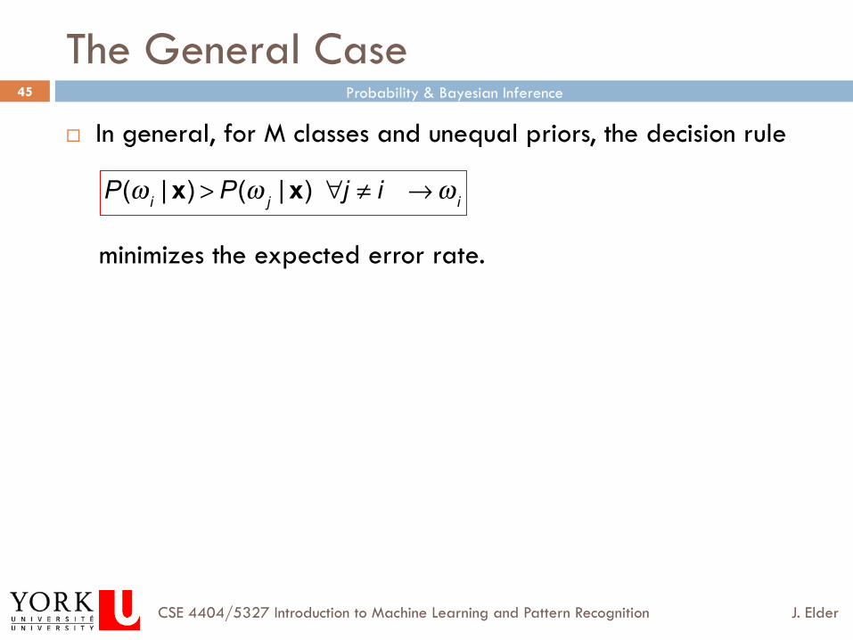
¨ In general, for M classes and unequal priors, the decision rule minimizes the expected error rate.
The General Case
45
P(ω i | x) > P(ω j | x) ∀j ≠ i →ω i

Probability & Bayesian Inference
J. Elder CSE 4404/5327 Introduction to Machine Learning and Pattern Recognition
46
Types of Error
¨ Minimizing the expected error rate is a pretty reasonable goal.
¨ However, it is not always the best thing to do. ¨ Example:
¤ You are designing a pedestrian detection algorithm for an autonomous navigation system.
¤ Your algorithm must decide whether there is a pedestrian crossing the street.
¤ There are two possible types of error: n False positive: there is no pedestrian, but the system thinks there
is. n Miss: there is a pedestrian, but the system thinks there is not.
¤ Should you give equal weight to these 2 types of error?
Probability & Bayesian Inference
J. Elder CSE 4404/5327 Introduction to Machine Learning and Pattern Recognition
47
Bayesian Decision Theory: Topics
1. Probability 2. The Univariate Normal Distribution 3. Bayesian Classifiers 4. Minimizing Risk
5. Nonparametric Density Estimation 6. Training and Evaluation Methods
Topic 4. Minimizing Risk
Probability & Bayesian Inference
J. Elder CSE 4404/5327 Introduction to Machine Learning and Pattern Recognition
49
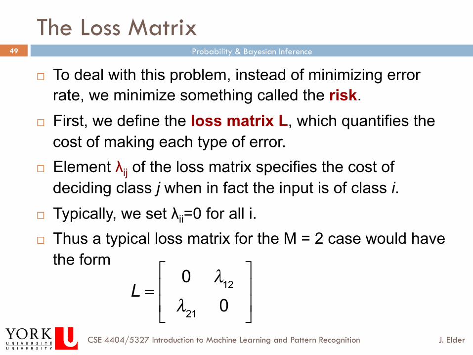
The Loss Matrix
¨ To deal with this problem, instead of minimizing error rate, we minimize something called the risk.
¨ First, we define the loss matrix L, which quantifies the cost of making each type of error.
¨ Element λij of the loss matrix specifies the cost of deciding class j when in fact the input is of class i.
¨ Typically, we set λii=0 for all i. ¨ Thus a typical loss matrix for the M = 2 case would have
the form
L =0 λ12
λ21 0
⎡
⎣⎢⎢
⎤
⎦⎥⎥
Probability & Bayesian Inference
J. Elder CSE 4404/5327 Introduction to Machine Learning and Pattern Recognition
50
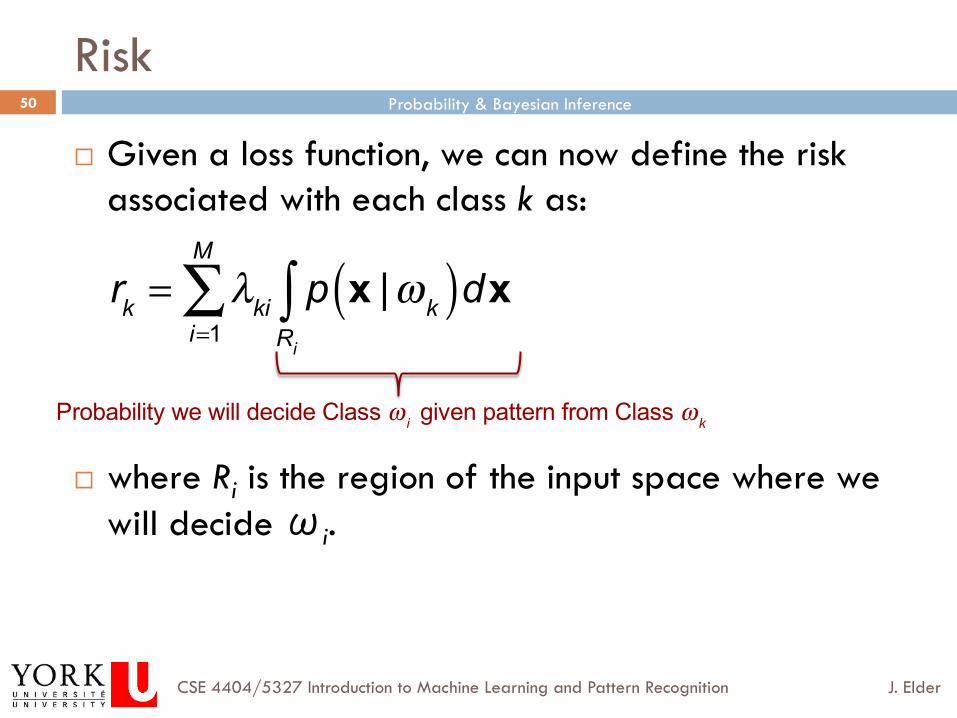
Risk
¨ Given a loss function, we can now define the risk associated with each class k as:
¨ where Ri is the region of the input space where we will decide ωi.
rk = λki p x |ωk( )dx
Ri
∫i=1
M
∑
Probability we will decide Class ω i given pattern from Class ωk
Probability & Bayesian Inference
J. Elder CSE 4404/5327 Introduction to Machine Learning and Pattern Recognition
51
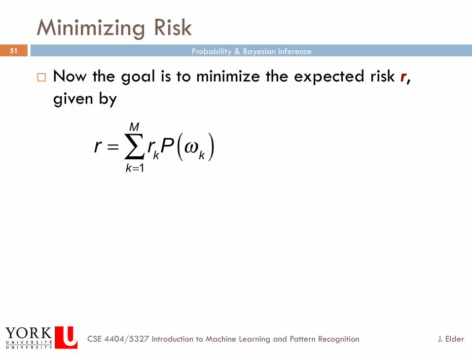
Minimizing Risk
¨ Now the goal is to minimize the expected risk r, given by
r = rkP ωk( )
k=1
M
∑
Probability & Bayesian Inference
J. Elder CSE 4404/5327 Introduction to Machine Learning and Pattern Recognition
52
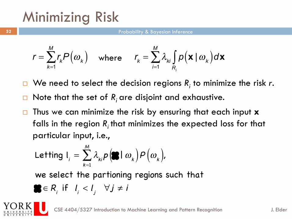
Minimizing Risk
¨ We need to select the decision regions Ri to minimize the risk r. ¨ Note that the set of Ri are disjoint and exhaustive.
¨ Thus we can minimize the risk by ensuring that each input x falls in the region Ri that minimizes the expected loss for that particular input, i.e.,
r = rkP ωk( )
k=1
M
∑ rk = λki p x |ωk( )dx
Ri
∫i=1
M
∑
Letting li = λki p x | ωk( )P ωk( )k=1
M∑ ,
we select the partioning regions such thatx ∈Ri if li < lj ∀j ≠ i
where
Probability & Bayesian Inference
J. Elder CSE 4404/5327 Introduction to Machine Learning and Pattern Recognition
53
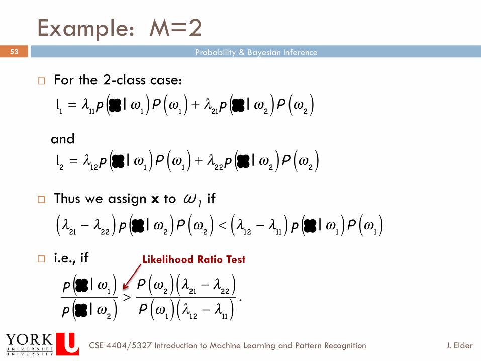
Example: M=2
¨ For the 2-class case:
and
¨ Thus we assign x to ω1 if
¨ i.e., if
l1 = λ11p x | ω 1( )P ω 1( ) + λ21p x | ω2( )P ω2( )
l2 = λ12p x | ω 1( )P ω 1( ) + λ22p x | ω2( )P ω2( )
λ21 − λ22( ) p x | ω2( )P ω2( ) < λ12 − λ11( ) p x | ω 1( )P ω 1( )
p x | ω 1( )p x | ω2( ) >
P ω2( ) λ21 − λ22( )P ω 1( ) λ12 − λ11( ) .
Likelihood Ratio Test
Probability & Bayesian Inference
J. Elder CSE 4404/5327 Introduction to Machine Learning and Pattern Recognition
54
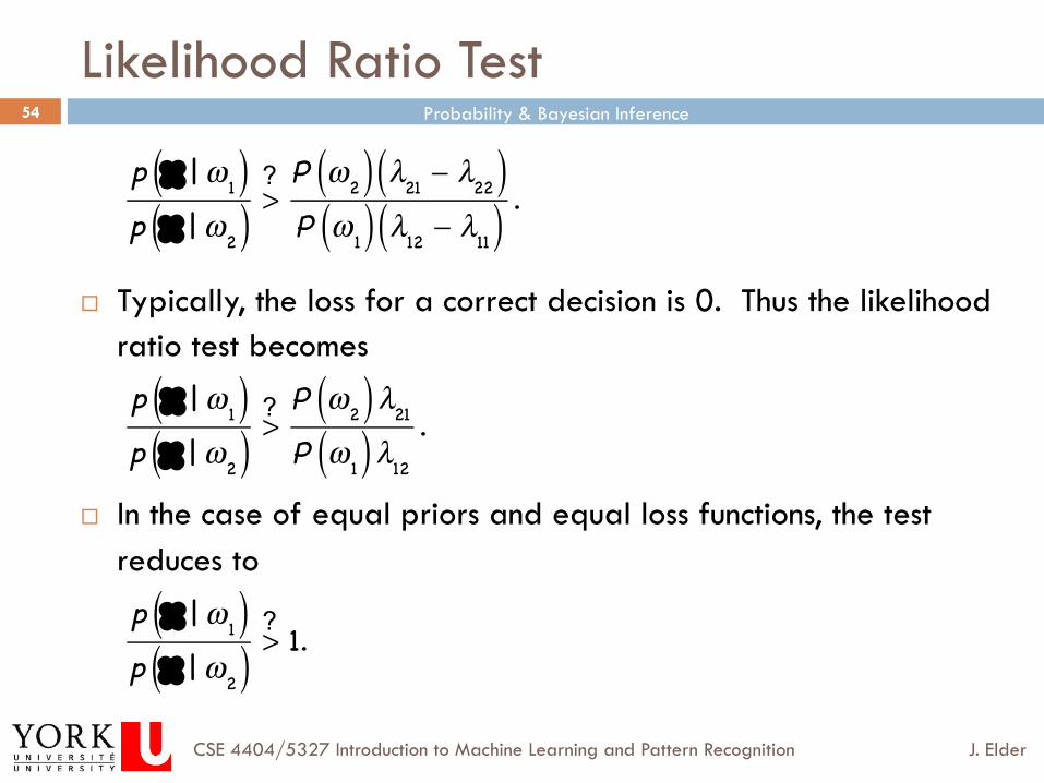
Likelihood Ratio Test
¨ Typically, the loss for a correct decision is 0. Thus the likelihood ratio test becomes
¨ In the case of equal priors and equal loss functions, the test reduces to
p x | ω 1( )p x | ω2( ) >
P ω2( ) λ21 − λ22( )P ω 1( ) λ12 − λ11( ) .
p x | ω 1( )p x | ω2( ) >
P ω2( )λ21
P ω 1( )λ12
.
p x | ω 1( )p x | ω2( ) > 1.
?
?
?
Probability & Bayesian Inference
J. Elder CSE 4404/5327 Introduction to Machine Learning and Pattern Recognition
55
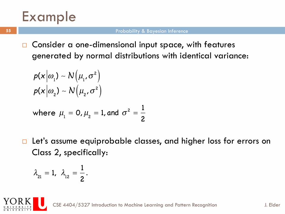
Example
¨ Consider a one-dimensional input space, with features generated by normal distributions with identical variance:
where
¨ Let’s assume equiprobable classes, and higher loss for errors on Class 2, specifically:
p(x ω 1 ) N µ1 ,σ 2( )p(x ω2 ) N µ2 ,σ 2( )
µ1 = 0, µ2 = 1, and σ 2 = 1
2
λ21 = 1, λ12 = 1
2 .
Probability & Bayesian Inference
J. Elder CSE 4404/5327 Introduction to Machine Learning and Pattern Recognition
56
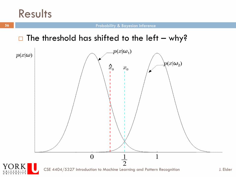
Results
¨ The threshold has shifted to the left – why?

Sept 12, 2012
End of Lecture
Probability & Bayesian Inference
J. Elder CSE 4404/5327 Introduction to Machine Learning and Pattern Recognition
58
Bayesian Decision Theory: Topics
1. Probability 2. The Univariate Normal Distribution 3. Bayesian Classifiers 4. Minimizing Risk 5. Nonparametric Density Estimation
6. Training and Evaluation Methods
Probability & Bayesian Inference
J. Elder CSE 4404/5327 Introduction to Machine Learning and Pattern Recognition
59
Nonparametric Methods
¨ Parametric distribution models are restricted to specific forms, which may not always be suitable; for example, consider modelling a multimodal distribution with a single, unimodal model.
¨ You can use a mixture model, but then you have to decide on the number of components, and hope that your parameter estimation algorithm (e.g., EM) converges to a global optimum!
¨ Nonparametric approaches make few assumptions about the overall shape of the distribution being modelled, and in some cases may be simpler than using a mixture model.
Probability & Bayesian Inference
J. Elder CSE 4404/5327 Introduction to Machine Learning and Pattern Recognition
60
Histogramming
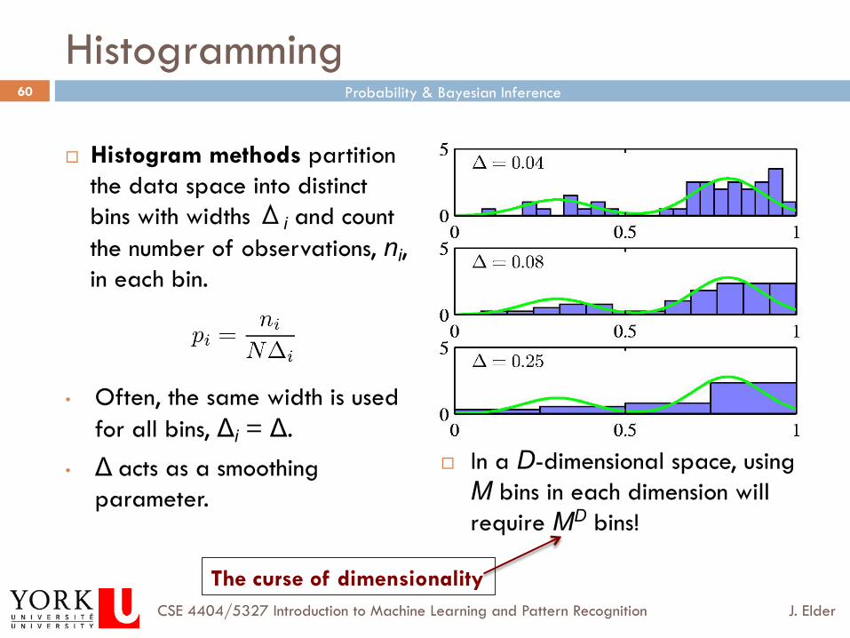
¨ Histogram methods partition the data space into distinct bins with widths Δi and count the number of observations, ni, in each bin.
• Often, the same width is used for all bins, Δi = Δ.
• Δ acts as a smoothing parameter.
¨ In a D-dimensional space, using M bins in each dimension will require MD bins!
The curse of dimensionality
Probability & Bayesian Inference
J. Elder CSE 4404/5327 Introduction to Machine Learning and Pattern Recognition
61
Kernel Density Estimation
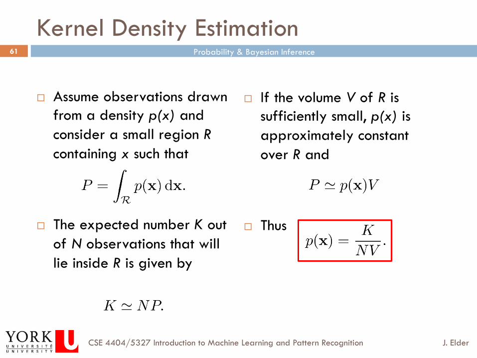
¨ Assume observations drawn from a density p(x) and consider a small region R containing x such that
¨ The expected number K out of N observations that will lie inside R is given by
¨ If the volume V of R is sufficiently small, p(x) is approximately constant over R and
¨ Thus
Probability & Bayesian Inference
J. Elder CSE 4404/5327 Introduction to Machine Learning and Pattern Recognition
62
Kernel Density Estimation
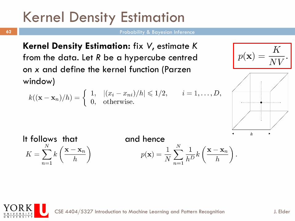
Kernel Density Estimation: fix V, estimate K from the data. Let R be a hypercube centred on x and define the kernel function (Parzen window)
It follows that and hence
Probability & Bayesian Inference
J. Elder CSE 4404/5327 Introduction to Machine Learning and Pattern Recognition
63
Kernel Density Estimation
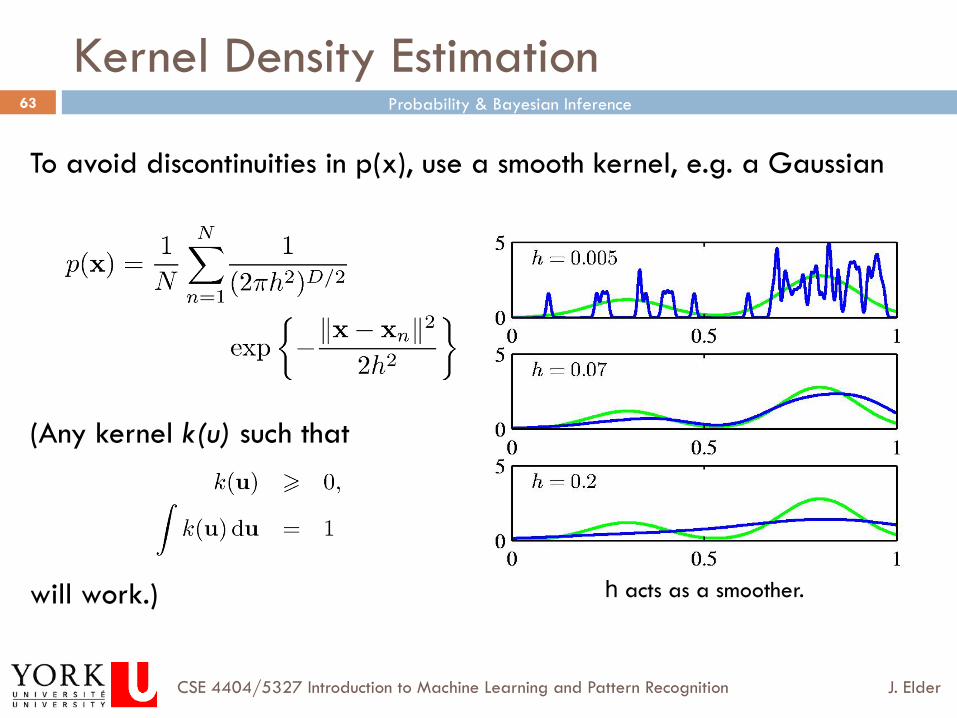
To avoid discontinuities in p(x), use a smooth kernel, e.g. a Gaussian
(Any kernel k(u) such that
will work.) h acts as a smoother.
Probability & Bayesian Inference
J. Elder CSE 4404/5327 Introduction to Machine Learning and Pattern Recognition
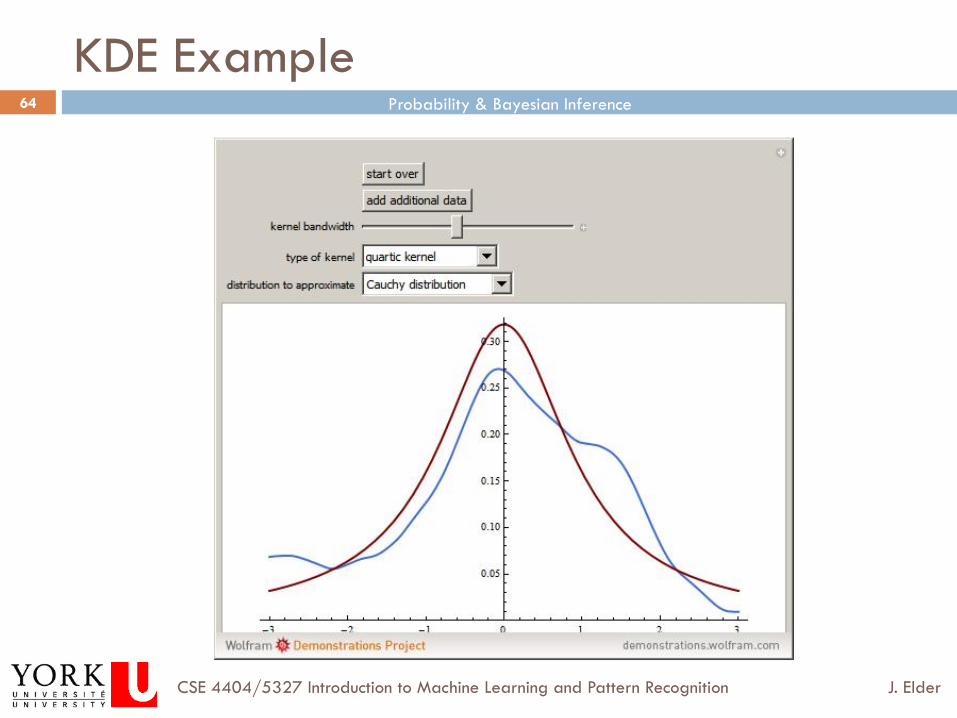
64
KDE Example
Probability & Bayesian Inference
J. Elder CSE 4404/5327 Introduction to Machine Learning and Pattern Recognition
65
Kernel Density Estimation
¨ Problem: if V is fixed, there may be too few points in some regions to get an accurate estimate.
Probability & Bayesian Inference
J. Elder CSE 4404/5327 Introduction to Machine Learning and Pattern Recognition
66
Nearest Neighbour Density Estimation
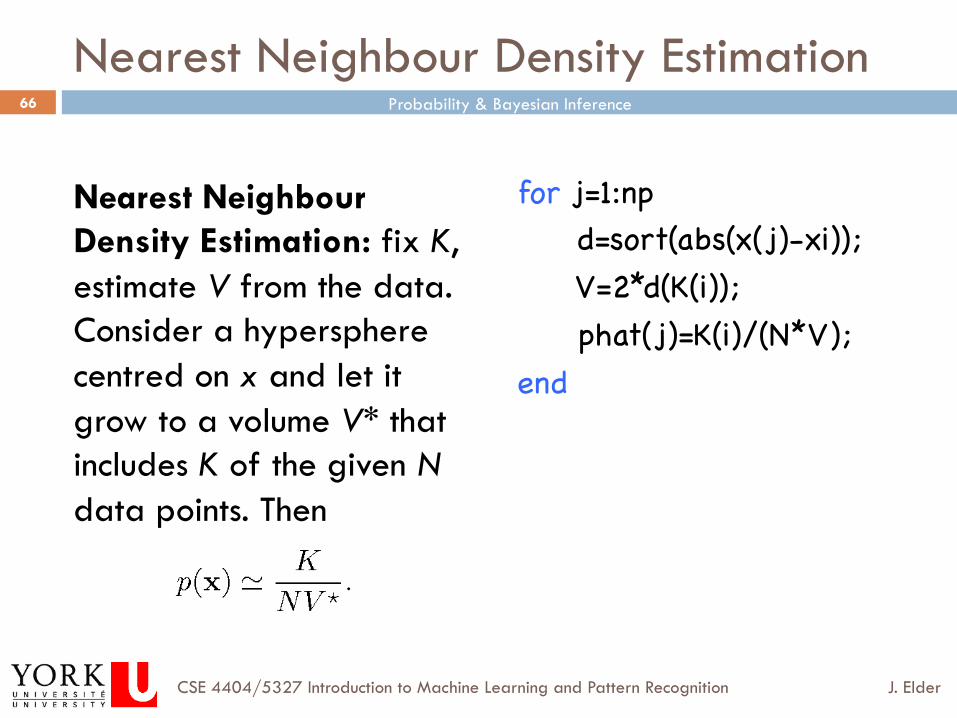
Nearest Neighbour Density Estimation: fix K, estimate V from the data. Consider a hypersphere centred on x and let it grow to a volume V* that includes K of the given N data points. Then
for j=1:np � d=sort(abs(x(j)-xi)); � V=2*d(K(i)); � phat(j)=K(i)/(N*V); �end�
Probability & Bayesian Inference
J. Elder CSE 4404/5327 Introduction to Machine Learning and Pattern Recognition
67
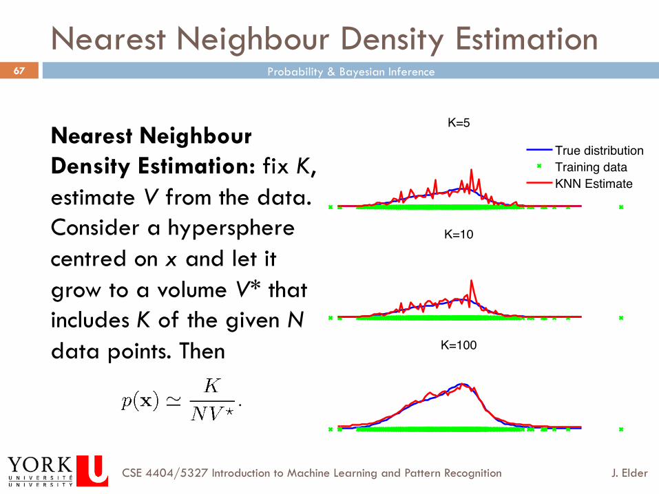
Nearest Neighbour Density Estimation
Nearest Neighbour Density Estimation: fix K, estimate V from the data. Consider a hypersphere centred on x and let it grow to a volume V* that includes K of the given N data points. Then
K=5
True distributionTraining dataKNN Estimate
K=10
K=100
Probability & Bayesian Inference
J. Elder CSE 4404/5327 Introduction to Machine Learning and Pattern Recognition
68
Nearest Neighbour Density Estimation
¨ Problem: does not generate a proper density (for example, integral is unbounded on )
¨ In practice, on finite domains, can normalize. ¨ But makes strong assumption on tails
D
∝1
x
⎛⎝⎜
⎞⎠⎟
Probability & Bayesian Inference
J. Elder CSE 4404/5327 Introduction to Machine Learning and Pattern Recognition
69
Nonparametric Methods
¨ Nonparametric models (not histograms) require storing and computing with the entire data set.
¨ Parametric models, once fitted, are much more efficient in terms of storage and computation.
Probability & Bayesian Inference
J. Elder CSE 4404/5327 Introduction to Machine Learning and Pattern Recognition
70
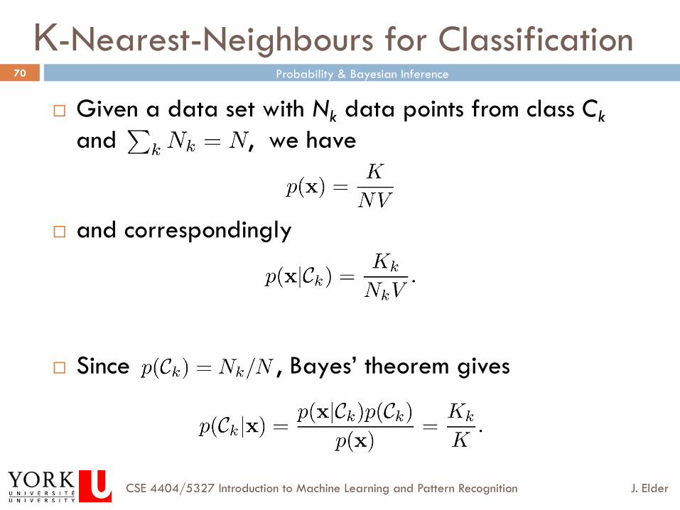
K-Nearest-Neighbours for Classification
¨ Given a data set with Nk data points from class Ck and , we have
¨ and correspondingly
¨ Since , Bayes’ theorem gives
Probability & Bayesian Inference
J. Elder CSE 4404/5327 Introduction to Machine Learning and Pattern Recognition
71
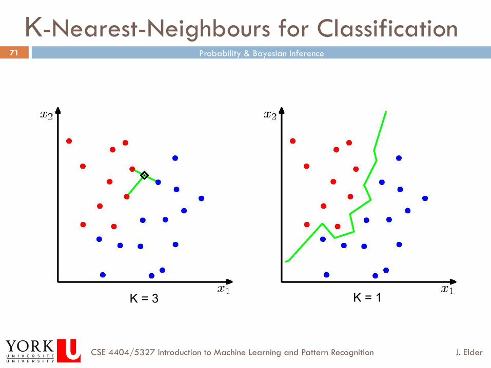
K-Nearest-Neighbours for Classification
K = 1 K = 3
Probability & Bayesian Inference
J. Elder CSE 4404/5327 Introduction to Machine Learning and Pattern Recognition
72
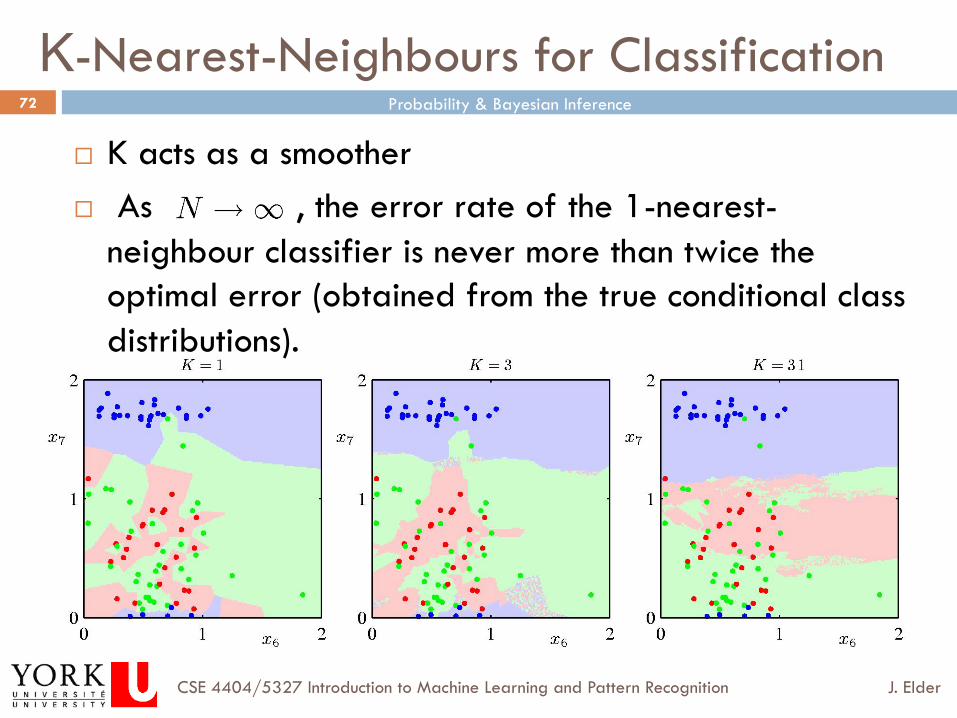
¨ K acts as a smoother ¨ As , the error rate of the 1-nearest-
neighbour classifier is never more than twice the optimal error (obtained from the true conditional class distributions).
K-Nearest-Neighbours for Classification
Probability & Bayesian Inference
J. Elder CSE 4404/5327 Introduction to Machine Learning and Pattern Recognition
73
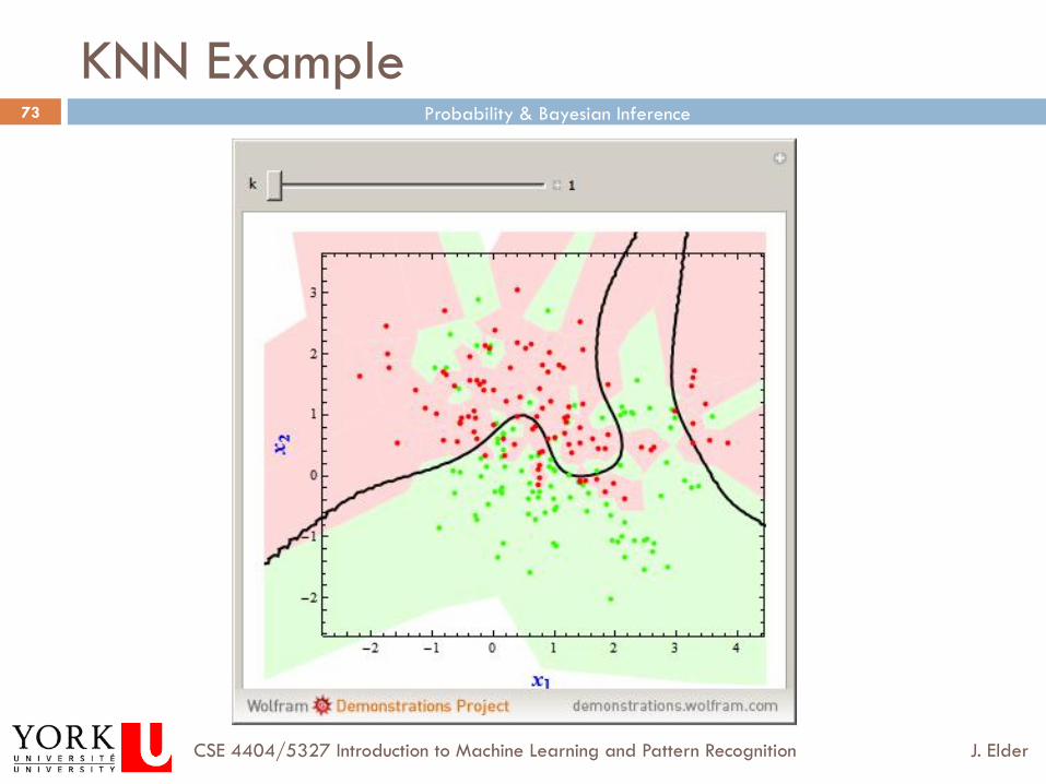
KNN Example
Probability & Bayesian Inference
J. Elder CSE 4404/5327 Introduction to Machine Learning and Pattern Recognition
74
Naïve Bayes Classifiers
¨ All of these nonparametric methods require lots of data to work. If training points are required for accurate estimation in 1 dimension, then points are required for D-dimensional input vectors.
¨ It may sometimes be possible to assume that the individual dimensions of the feature vector are conditionally independent. Then we have
¨ This reduces the data requirements to p x | ω i( ) = p xj | ω i( )
j =1
D∏
O ND( )
O DN( ) .
O N( )
Probability & Bayesian Inference
J. Elder CSE 4404/5327 Introduction to Machine Learning and Pattern Recognition
75
Bayesian Decision Theory: Topics
1. Probability 2. The Univariate Normal Distribution 3. Bayesian Classifiers 4. Minimizing Risk 5. Nonparametric Density Estimation 6. Training and Evaluation Methods
Probability & Bayesian Inference
J. Elder CSE 4404/5327 Introduction to Machine Learning and Pattern Recognition
76
Machine Learning System Design
¨ The process of solving a particular classification or regression problem typically involves the following sequence of steps: 1. Design and code promising candidate systems 2. Train each of the candidate systems (i.e., learn the
parameters) 3. Evaluate each of the candidate systems 4. Select and deploy the best of these candidate systems
Probability & Bayesian Inference
J. Elder CSE 4404/5327 Introduction to Machine Learning and Pattern Recognition
77
Using Your Training Data
¨ You will always have a finite amount of data on which to train and evaluate your systems.
¨ The performance of a classification system is often data-limited: if we only had more data, we could make the system better.
¨ Thus it is important to use your finite data set wisely.
Probability & Bayesian Inference
J. Elder CSE 4404/5327 Introduction to Machine Learning and Pattern Recognition
78
Overfitting
¨ Given that learning is often data-limited, it is tempting to use all of your data to estimate the parameters of your models, and then select the model with the lowest error on your training data.
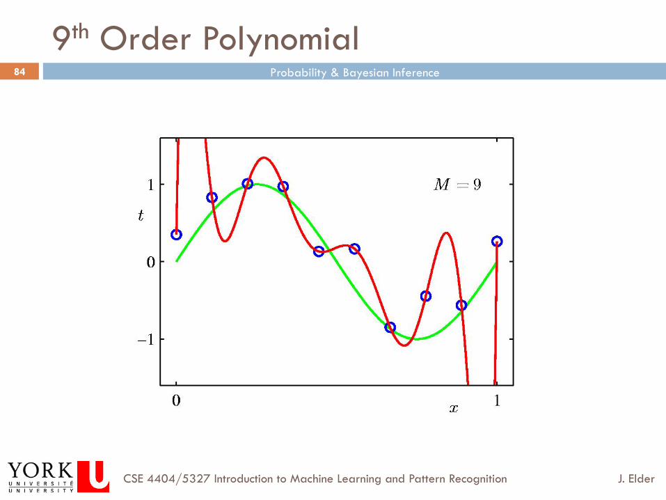
¨ Unfortunately, this leads to a notorious problem called over-fitting.
Probability & Bayesian Inference
J. Elder CSE 4404/5327 Introduction to Machine Learning and Pattern Recognition
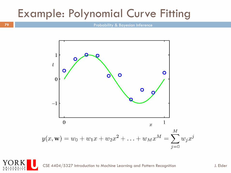
79
Example: Polynomial Curve Fitting
Probability & Bayesian Inference
J. Elder CSE 4404/5327 Introduction to Machine Learning and Pattern Recognition
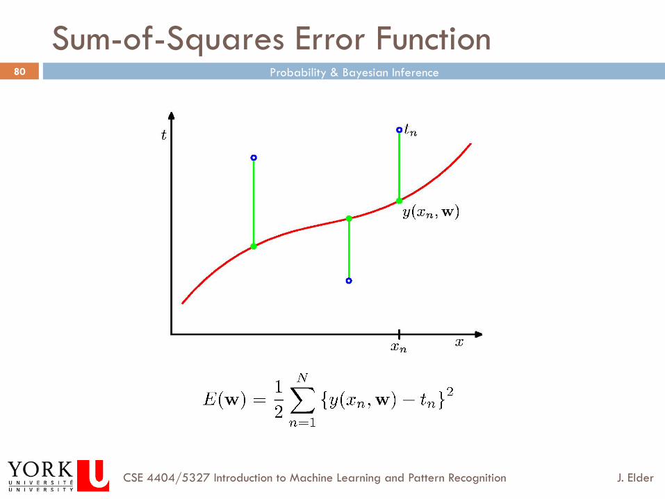
80
Sum-of-Squares Error Function
Probability & Bayesian Inference
J. Elder CSE 4404/5327 Introduction to Machine Learning and Pattern Recognition
81
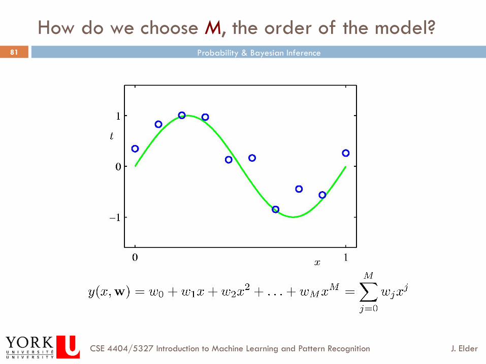
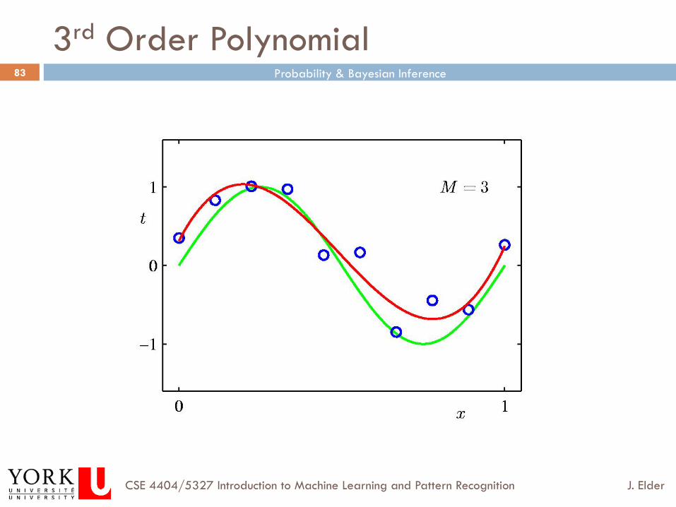
How do we choose M, the order of the model?
Probability & Bayesian Inference
J. Elder CSE 4404/5327 Introduction to Machine Learning and Pattern Recognition
82
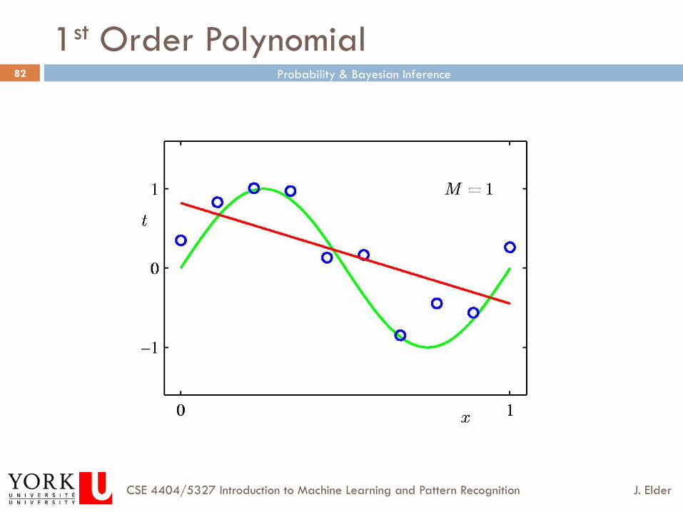
1st Order Polynomial
Probability & Bayesian Inference
J. Elder CSE 4404/5327 Introduction to Machine Learning and Pattern Recognition
83
3rd Order Polynomial
Probability & Bayesian Inference
J. Elder CSE 4404/5327 Introduction to Machine Learning and Pattern Recognition
84
9th Order Polynomial
Probability & Bayesian Inference
J. Elder CSE 4404/5327 Introduction to Machine Learning and Pattern Recognition
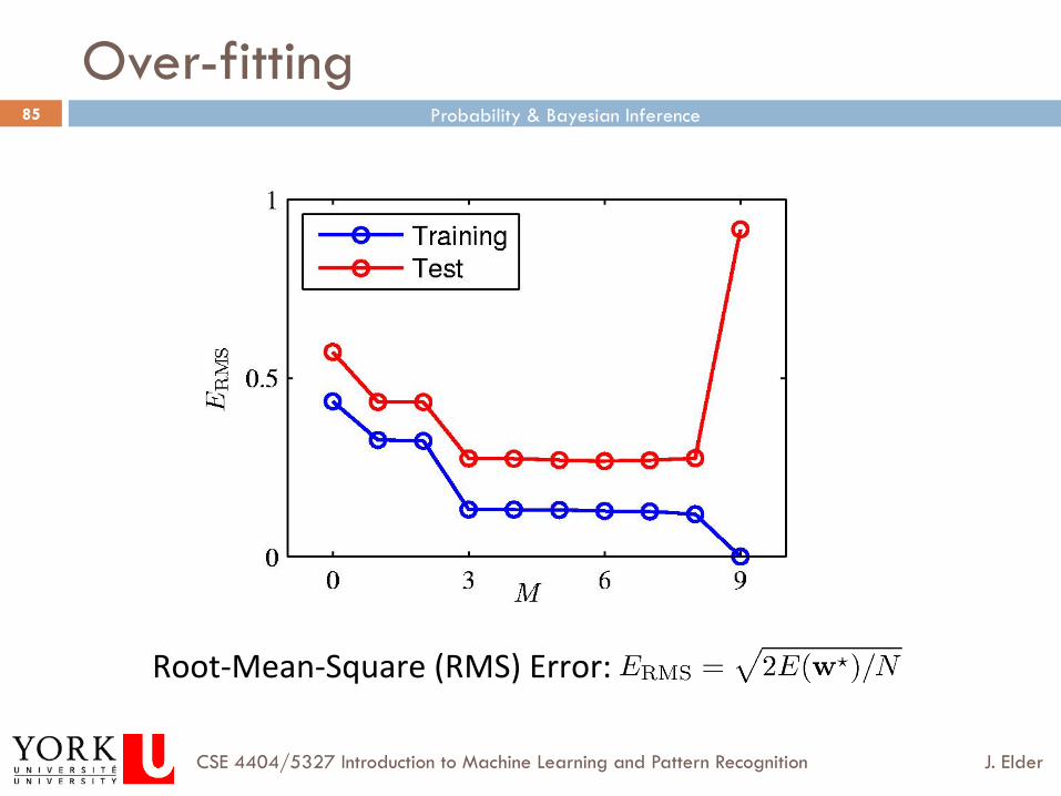
85
Over-fitting
Root-‐Mean-‐Square (RMS) Error:
Probability & Bayesian Inference
J. Elder CSE 4404/5327 Introduction to Machine Learning and Pattern Recognition
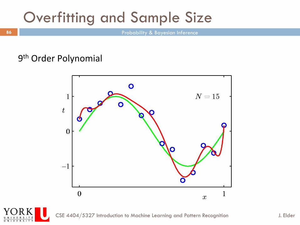
86
Overfitting and Sample Size
9th Order Polynomial
Probability & Bayesian Inference
J. Elder CSE 4404/5327 Introduction to Machine Learning and Pattern Recognition
87
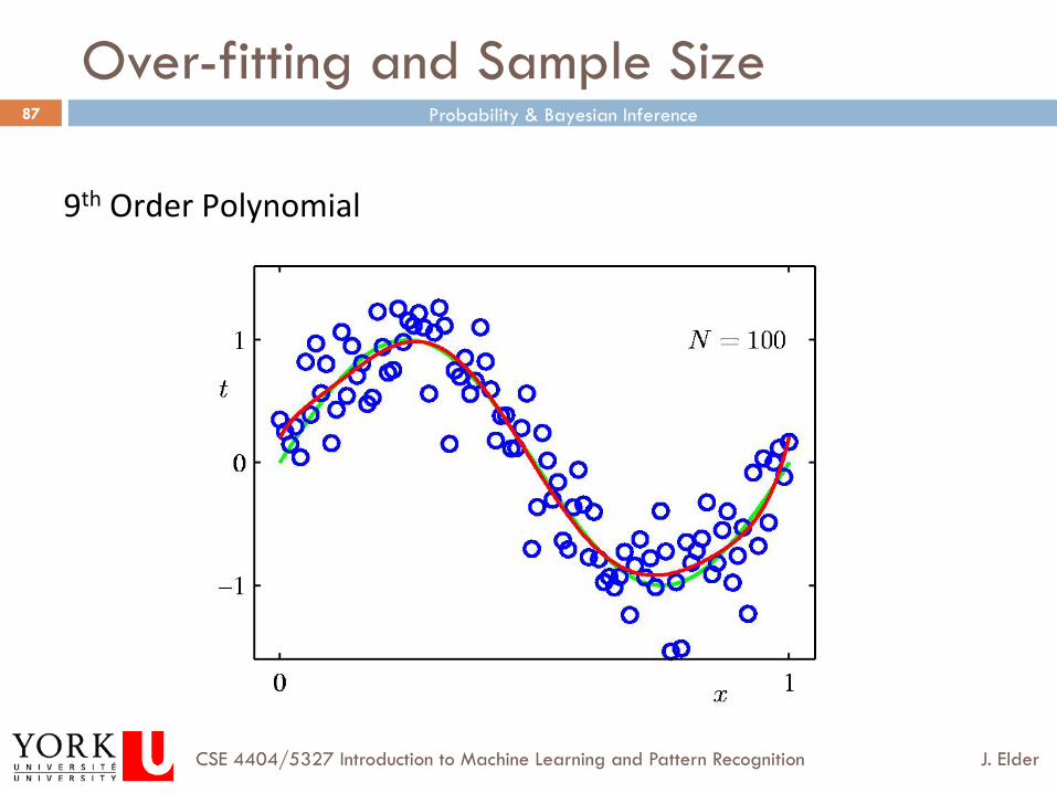
Over-fitting and Sample Size
9th Order Polynomial
Probability & Bayesian Inference
J. Elder CSE 4404/5327 Introduction to Machine Learning and Pattern Recognition
88
Methods for Preventing Over-Fitting
¨ Bayesian parameter estimation ¤ Application of prior knowledge regarding the probable
values of unknown parameters can often limit over-fitting of a model
¨ Model selection criteria ¤ Methods exist for comparing models of differing complexity
(i.e., with different types and numbers of parameters) n Bayesian Information Criterion (BIC) n Akaike Information Criterion (AIC)
¨ Cross-validation ¤ This is a very simple method that is universally applicable.
Probability & Bayesian Inference
J. Elder CSE 4404/5327 Introduction to Machine Learning and Pattern Recognition
89
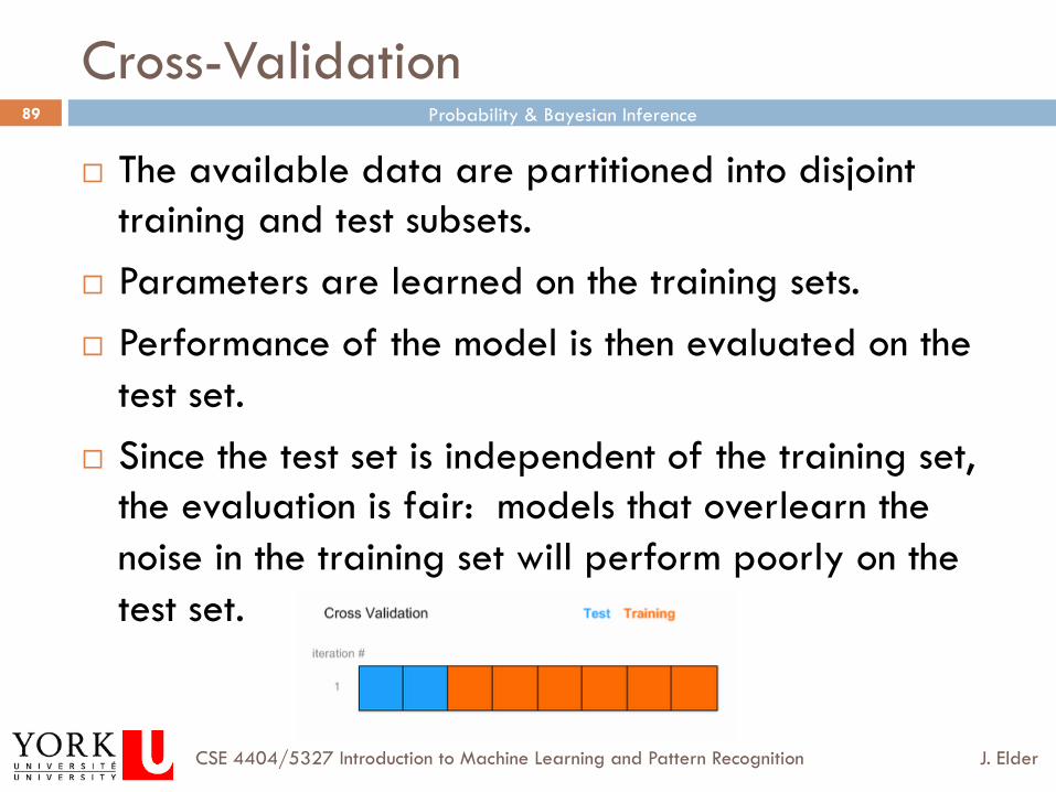
Cross-Validation
¨ The available data are partitioned into disjoint training and test subsets.
¨ Parameters are learned on the training sets. ¨ Performance of the model is then evaluated on the
test set. ¨ Since the test set is independent of the training set,
the evaluation is fair: models that overlearn the noise in the training set will perform poorly on the test set.
Probability & Bayesian Inference
J. Elder CSE 4404/5327 Introduction to Machine Learning and Pattern Recognition
90
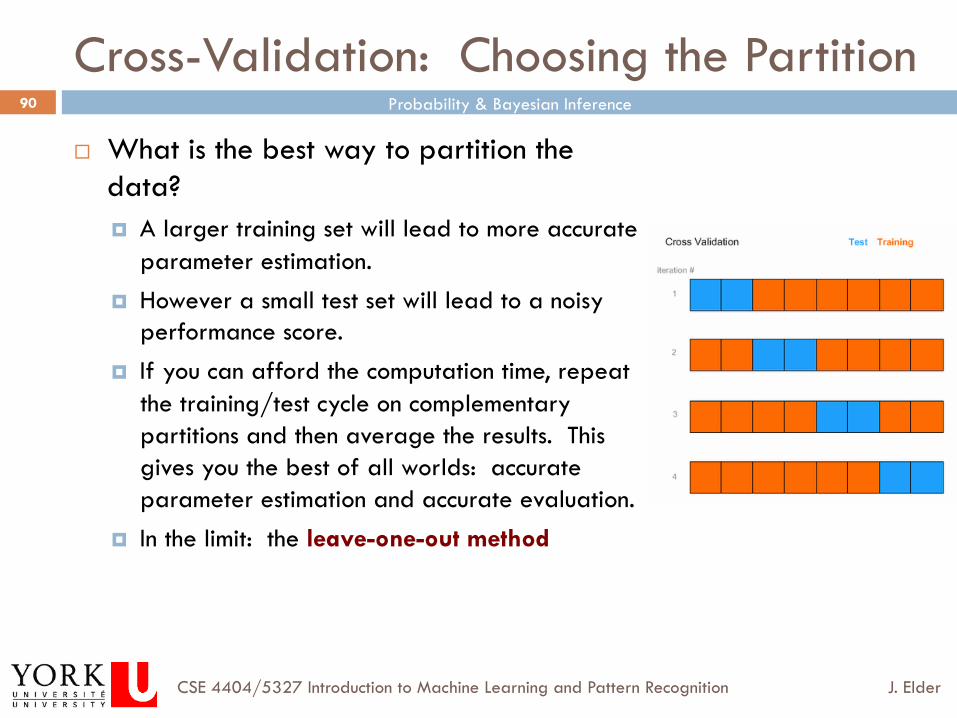
Cross-Validation: Choosing the Partition
¨ What is the best way to partition the data? ¤ A larger training set will lead to more accurate
parameter estimation. ¤ However a small test set will lead to a noisy
performance score. ¤ If you can afford the computation time, repeat
the training/test cycle on complementary partitions and then average the results. This gives you the best of all worlds: accurate parameter estimation and accurate evaluation.
¤ In the limit: the leave-one-out method
Probability & Bayesian Inference
J. Elder CSE 4404/5327 Introduction to Machine Learning and Pattern Recognition
91
A useful MATLAB function
¨ randperm(n) ¤ Generates a random permutation of the integers from
1 to n ¤ The result can be used to select random subsets from
your data

Probability & Bayesian Inference
J. Elder CSE 4404/5327 Introduction to Machine Learning and Pattern Recognition
92
Bayesian Decision Theory: Topics
1. Probability 2. The Univariate Normal Distribution 3. Bayesian Classifiers 4. Minimizing Risk 5. Nonparametric Density Estimation 6. Training and Evaluation Methods