bayesian doubly adaptive elastic-net lasso for var shrinkage

Bayesian Doubly Adaptive Elastic-Net Lasso For

VAR Shrinkage

Deborah Gefang∗

Department of Economics

University of Lancaster

email: [email protected]

January 10, 2012

Abstract

We develop a novel Bayesian doubly adaptive elastic-net Lasso(DAELasso) approach for VAR shrinkage. DAELasso achieves dataselection and coefficients shrinkage in a data based manner. It con-structively deals with the explanatory variables that tend to be highlycollinear by encouraging grouping effect. In addition, it allows for dif-ferent degree of shrinkages for different coefficients. Rewriting the mul-tivariate Laplace distribution as a scale mixture, we establish closed-form posteriors that can be drawn from a Gibbs sampler. We comparethe forecasting performance of DAELasso to that of other popularBayesian methods using US macro economic data. The results suggestthat DAELasso is a useful complement to the available Baysian VARshrinkage methods.

∗The author would like to thank Gary Koop and participants of CFE11 conference inLondon for their constructive comments. Any remaining errors are the author’s responsi-bility.

1

1 Introduction

Since the seminal work of Sims (1972, 1980), vector autoregressive (VAR)

models have been widely used for analyzing the interrelationship between

economic series and forecasting. VAR models are parameter rich and sub-

ject to the curse of dimensionality. With the increasing availability of data,

it is not uncommon for researchers to have a VAR with the number of coef-

ficients exceeding the number of observations. In this case, the coefficients

can no longer be uniquely estimated. Various Bayesian shrinkage methods

have proved successful in circumventing this problem by imposing appropri-

ate prior restrictions. Following the notion of Chudik and Pesaran (2011),

we can divide the popular Bayesian VAR shrinkage approaches into three

categories: (i) shrinkage of the parameter space, (ii) shrinkage of the vari-

able space, and (iii) shrinkage of both the parameter space and variable

space. Traditional Minnesota prior of Doan et al (1984) and Litterman

(1986) and its natural variants (e.g. Kadiyala and Karlsson, 1997; Banbura

et al, 2010), shrink the parameters through priors controlling the degree of

shrinkage. The stochastic search variable selection (SSVS) prior of George

et al (2008) shrinks variable space by including/excluding different explana-

tory variables. Finally, the family of SSVS plus Minnesota priors of Koop

(2011) combine variable selection and parameter shrinkage.

Despite being successful, these Bayesian VAR shrinkage methods have

their own drawbacks. A main feature of Minnesota priors is that they dis-

criminate between the parameters on own lags and that on lags of other

variables. By doing so, Minnesota priors risk diminishing the effects of

2

possible leading indicators and coincident variables, whose importance for

forecasting has been intensively investigated since first being advocated by

Burns and Mitchell at the National Bureau of Economic Research in 1937

(e.g. Burns and Mitchell, 1946; Stock and Watson, 1989). By contrast,

SSVS prior for VAR is not subject to the criticism of being subjective as it

relies on data information to select variables. Yet, SSVS VAR prior is devel-

oped from its single equation counterpart of George and McCulloch (1993,

1997), and in the single equation set-up, standard SSVS prior is known for

tending to select highly correlated variables at the cost of ignoring others

that may improve the model’s forecasting performance (Kwon et al, 2011).

Tibshirani’s (1996) least absolute shrinkage and selection operator (Lasso)

and its variants, such as fused Lasso of Tibshirani et al (2005), elastic net

Lasso (e-net Lasso) of Zou and Hastie (2005), and grouped Lasso of Yuan

and Lin (2007), offer the potential for alternative approaches to VAR shrink-

age. Lasso methods are attractive as they can select variables and shrink

parameters in a data based manner. Recently, Bayesian Lasso has gained

popularity as it can be easily implemented through MCMC or a Gibbs sam-

pler (e.g. Park and Casella, 2008; Kyung et al, 2010), and it can automat-

ically achieve adaptive shrinkage to allow for different degree of shrinkage

(e.g. Griffin and Brown, 2010; Leng et al, 2010). Despite being successful,

the Lasso literature is mainly concentrated on single equation models. To

our best knowledge, only a few studies in the frequentist framework explore

Lasso shrinkage for VARs (e.g., Hsu, Hung and Chang, 2008; Song and

Bickel, 2011). And these available methods can be too restrictive as they

either assume the covariance matrix of the VAR errors to be diagonal or

3

assume its off-diagonal elements are much smaller than the diagonal ones.

This paper develops a novel Bayesian Lasso method for VAR shrinkage:

the doubly adaptive e-net Lasso (DAELasso) that suitable for VAR models

in macroeconomic research. Considering VAR models usually have highly

correlated explanatory variables and sometime have more coefficients than

the observations, we use the e-net Lasso of Zou and Hastie (2005) to deal

with the problem of multicollinearity. While Lasso generally only picks up

one variable among a group of highly correlated variables, e-net Lasso has

the potential of selecting all the important variables regardless the number

of observations (Zou and Hastie, 2005). Note that if we have formal and

informal economic theory at hand to group the data, it can be more desirable

to have other type of Lasso, such as the fused Lasso and grouped Lasso,

instead of e-net Lasso for VAR shrinkage. Yet in general we do not have

such information, and e-net Lasso turns out to be the most appealing choice

for it encourages the grouping effect supported by the data itself. Finally,

considering that the traditional e-net Lasso can give the wrong results as

it imposes the same amount of shrinkage for all the coefficients (Zou and

Zhang, 2009), we extend the Bayesian adaptive Lasso of Leng et al (2010) to

e-net Lasso. We call the approach ‘doubly adaptive’ to reflect the fact that

unlike the adaptive e-net Lasso of Zou and Zhang (2009) which only adapts

the tuning parameters of the L1 norm, we allow for tuning parameters of

both the L1 and L2 norms to be adapted. DAELasso is flexible, but it can

be too complicated for some data. Thus, in this paper we also introduce four

alternative Lasso types of VAR shrinkage methods: Lasso, adaptive Lasso,

e-net Lasso, and adaptive e-net Lasso, each of them is a nested version of

4

DAELasso.

In empirical work, we evaluate the forecasting performance of DAELasso

approach alongside Lasso, adaptive Lasso, e-net Lasso, and adaptive e-net

Lasso. In addition, we compare the forecasting performance of these Lasso

types of methods with that of other seven popular Baysian VAR shrinkage

methods reviewed in Koop (2011). We employ Koop’s (2011) data set that

contains 20 US macroeconomic series, which is originally compiled by James

H. Stock and Mark W. Watson. The data runs from 1959Q1 to 2008Q4.

In line with Koop (2011), we conduct rolling and recursive forecast exer-

cises and calculate both the mean squared forecast error (MSFE) and pre-

dictive likelihood measures. Using relatively uninformative priors, we find

DAELasso approach leads to forecasting results that compares favorably or

equally well to other Bayesian VAR shrinkage methods. This suggests that

DAELasso approach is an appropriate complement to the available Baysian

VAR toolkit.

The remainder of the paper is organized as following. Section 2 devel-

ops the Bayesian DAELasso methods. Section 3 presents four alternative

Lasso types of VAR shrinkage methods that nested in DAELasso. Section 4

compares the forecasting performance of Lasso methods and the seven pop-

ular Bayesian VAR shrinkage methods reviewed in Koop (2011). Section 5

concludes. A data list is provided in the appendix.

5

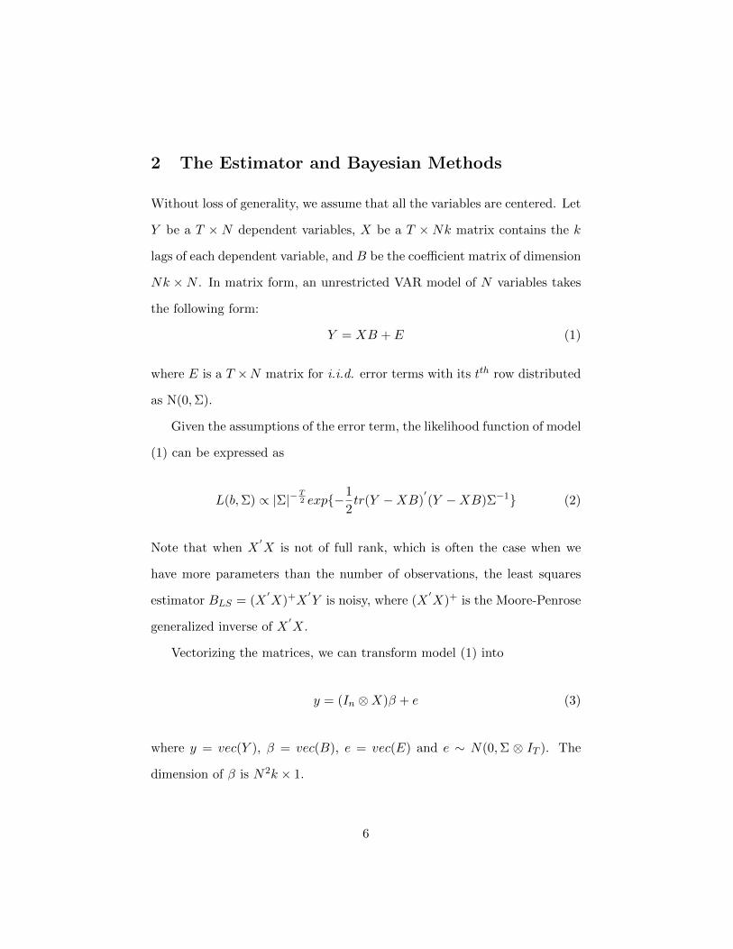
2 The Estimator and Bayesian Methods

Without loss of generality, we assume that all the variables are centered. Let

Y be a T × N dependent variables, X be a T × Nk matrix contains the k

lags of each dependent variable, and B be the coefficient matrix of dimension

Nk ×N . In matrix form, an unrestricted VAR model of N variables takes

the following form:

Y = XB + E (1)

where E is a T ×N matrix for i.i.d. error terms with its tth row distributed

as N(0,Σ).

Given the assumptions of the error term, the likelihood function of model

(1) can be expressed as

L(b,Σ) ∝ |Σ|−T2 exp{−1

2tr(Y −XB)

′(Y −XB)Σ−1} (2)

Note that when X′X is not of full rank, which is often the case when we

have more parameters than the number of observations, the least squares

estimator BLS = (X′X)+X

′Y is noisy, where (X

′X)+ is the Moore-Penrose

generalized inverse of X′X.

Vectorizing the matrices, we can transform model (1) into

y = (In ⊗X)β + e (3)

where y = vec(Y ), β = vec(B), e = vec(E) and e ∼ N(0,Σ ⊗ IT ). The

dimension of β is N2k × 1.

6

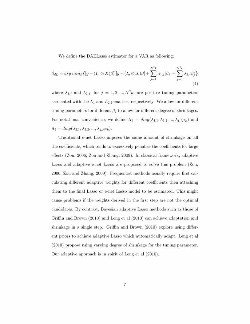
We define the DAELasso estimator for a VAR as following:

βdL = arg minβ{[y− (In⊗X)β]′[y− (In⊗X)β] +

N2k∑j=1

λ1,j |βj |+N2k∑j=1

λ2,jβ2j }

(4)

where λ1,j and λ2,j , for j = 1, 2, ..., N2k, are positive tuning parameters

associated with the L1 and L2 penalties, respectively. We allow for different

tuning parameters for different βj to allow for different degree of shrinkages.

For notational convenience, we define Λ1 = diag(λ1,1, λ1,2, ..., λ1,N2k) and

Λ2 = diag(λ2,1, λ2,2, ..., λ2,N2k).

Traditional e-net Lasso imposes the same amount of shrinkage on all

the coefficients, which tends to excessively penalize the coefficients for large

effects (Zou, 2006; Zou and Zhang, 2009). In classical framework, adaptive

Lasso and adaptive e-net Lasso are proposed to solve this problem (Zou,

2006; Zou and Zhang, 2009). Frequentist methods usually require first cal-

culating different adaptive weights for different coefficients then attaching

them to the final Lasso or e-net Lasso model to be estimated. This might

cause problems if the weights derived in the first step are not the optimal

candidates. By contrast, Bayesian adaptive Lasso methods such as those of

Griffin and Brown (2010) and Leng et al (2010) can achieve adaptation and

shrinkage in a single step. Griffin and Brown (2010) explore using differ-

ent priors to achieve adaptive Lasso which automatically adapt. Leng et al

(2010) propose using varying degree of shrinkage for the tuning parameter.

Our adaptive approach is in spirit of Leng et al (2010).

7

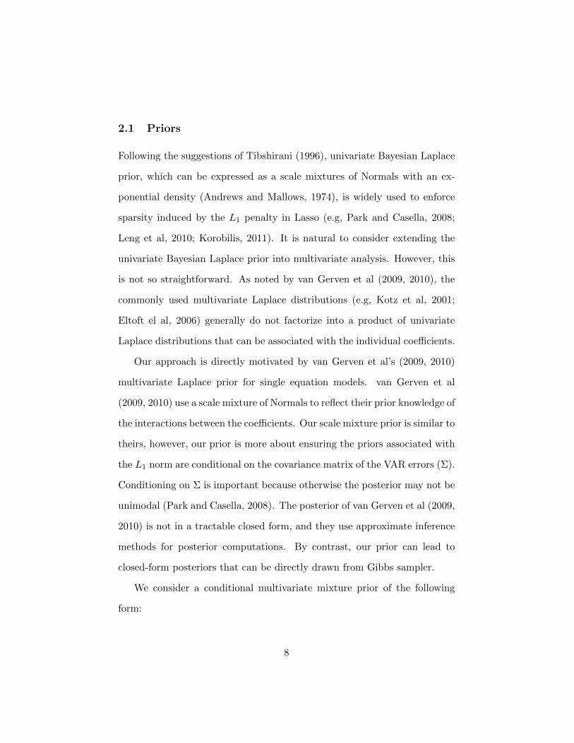
2.1 Priors

Following the suggestions of Tibshirani (1996), univariate Bayesian Laplace

prior, which can be expressed as a scale mixtures of Normals with an ex-

ponential density (Andrews and Mallows, 1974), is widely used to enforce

sparsity induced by the L1 penalty in Lasso (e.g, Park and Casella, 2008;

Leng et al, 2010; Korobilis, 2011). It is natural to consider extending the

univariate Bayesian Laplace prior into multivariate analysis. However, this

is not so straightforward. As noted by van Gerven et al (2009, 2010), the

commonly used multivariate Laplace distributions (e.g, Kotz et al, 2001;

Eltoft el al, 2006) generally do not factorize into a product of univariate

Laplace distributions that can be associated with the individual coefficients.

Our approach is directly motivated by van Gerven et al’s (2009, 2010)

multivariate Laplace prior for single equation models. van Gerven et al

(2009, 2010) use a scale mixture of Normals to reflect their prior knowledge of

the interactions between the coefficients. Our scale mixture prior is similar to

theirs, however, our prior is more about ensuring the priors associated with

the L1 norm are conditional on the covariance matrix of the VAR errors (Σ).

Conditioning on Σ is important because otherwise the posterior may not be

unimodal (Park and Casella, 2008). The posterior of van Gerven et al (2009,

2010) is not in a tractable closed form, and they use approximate inference

methods for posterior computations. By contrast, our prior can lead to

closed-form posteriors that can be directly drawn from Gibbs sampler.

We consider a conditional multivariate mixture prior of the following

form:

8

π(β|Σ,Γ,Λ1,Λ2) ∝N2k∏j=1

{√λ2,j√2π

exp(−λ2,j

2β2j )

×∫ ∞

0

1√2πfj(Γ))

exp[− 1

2fj(Γ)β2j ]d(fj(Γ))}

× {|M |−12 exp(−1

2Γ′M−1Γ)}2

(5)

where Γ = [γ1, γ2, ..., γN2k]′, M = Σ ⊗ INk, and fj(Γ) is a function of Γ

and Λ1 to be defined later. In this mixture prior, the terms associated with

the L1 penalty are conditional on Σ through fj(Γ). This is important as

otherwise the posterior will be not unimodal due to the ‘sharp corners’ of

the L1 penalty (Park and and Casella, 2008). In (5), the variances of βa

and βb for a 6= b are related through M . However, βa and βb themselves are

independent of each other.

We need to find an appropriate fj(Γ) which provides us tractable poste-

riors. The last term in (5) indicates that Γ ∼ N(0,M), with

M =

M1,1 ... M1,j M1,j+1 ... M1,N2k

... ... ... ... ... ...

Mj,1 ... Mj,j Mj,j+1 ... Mj,N2k

Mj+1,1 ... Mj+1,j Mj+1,j+1 ... Mj+1,N2k

... ... ... ... ... ...

MN2k,1 ... MN2k,j MN2k,j+1 ... MN2k,N2k

(6)

9

Let Hj = (Mj,j+1, ...,Mj,N2k)

Mj+1,j+1 ... Mj+1,N2k

... ... ...

MN2k,j+1 ... MN2k,N2k

−1

.

We next construct independent variables τj for j = 1, 2, ..., N2k using stan-

dard textbook techniques (e.g. Anderson, 2003; Muirhead 1982).

τ1 = γ1 +H1(γ2, γ3, ..., γN2k)′

(7)

τ2 = γ2 +H2(γ3, γ4, ..., γN2k)′

(8)

...

τN2K−1 = γN2k−1 +HN2k−1γN2k (9)

τN2K = γN2k (10)

The joint density of τ1, τ2, ...., τN2k is

N(τ1|0, σ2γ1)N(τ2|0, σ2

γ2)...N(τN2k|0, σ2γN2k

) (11)

where σ2γj = Mj,j −Hj(Mj,j+1, ...,Mj,N2k)

′, with σ2γN2k

= MN2k,N2k. Note

that it is computationally feasible to derive σ2γj when M is sparse.

The Jacobian of transforming Γ ∼ N(0,M) to (11) is 1. Defining ηj =

τj/λ1,j , we can write (11) as

N(η1|0, σ2γ1λ−21,1)N(η2|0, σ2

γ2λ−21,2)...N(ηN2k|0, σ2

γN2kλ−2

1,N2k) (12)

10

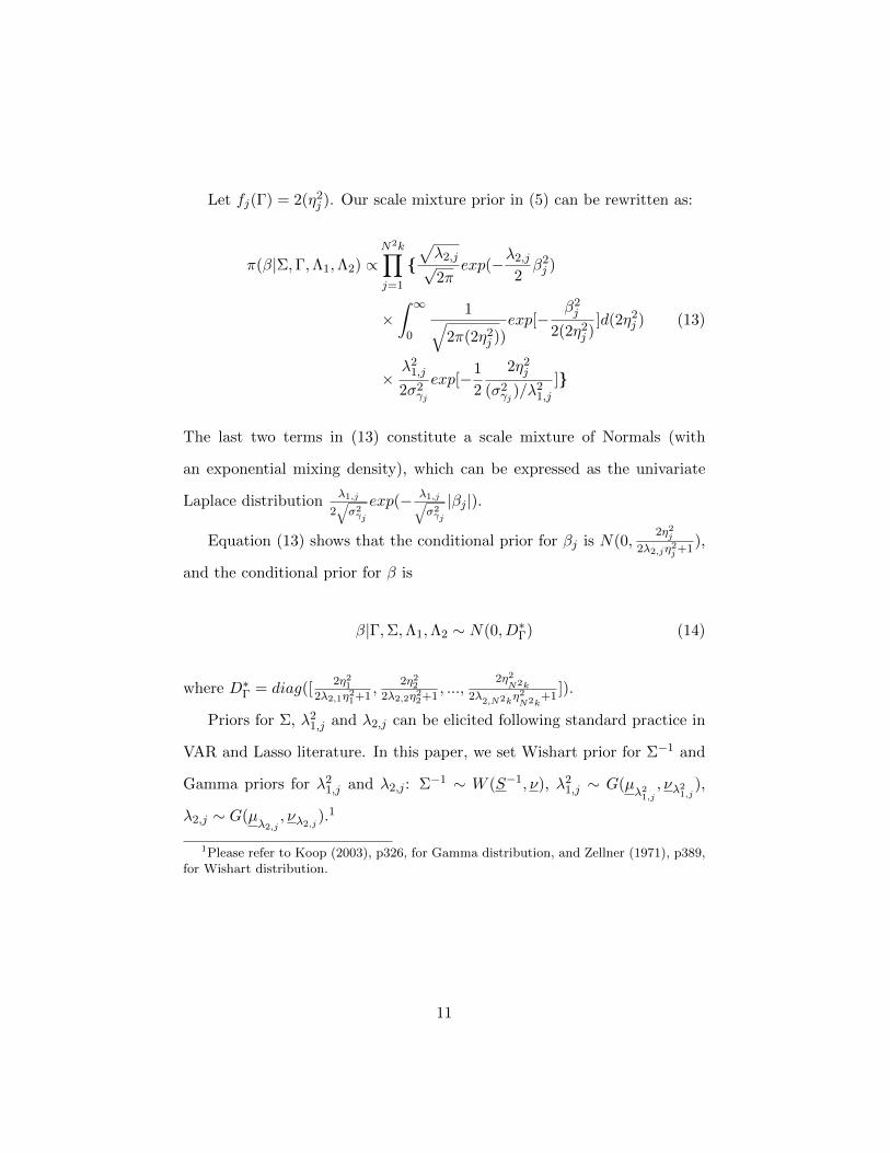
Let fj(Γ) = 2(η2j ). Our scale mixture prior in (5) can be rewritten as:

π(β|Σ,Γ,Λ1,Λ2) ∝N2k∏j=1

{√λ2,j√2π

exp(−λ2,j

2β2j )

×∫ ∞

0

1√2π(2η2

j ))exp[−

β2j

2(2η2j )

]d(2η2j )

×λ2

1,j

2σ2γj

exp[−1

2

2η2j

(σ2γj )/λ

21,j

]}

(13)

The last two terms in (13) constitute a scale mixture of Normals (with

an exponential mixing density), which can be expressed as the univariate

Laplace distributionλ1,j

2√σ2γj

exp(− λ1,j√σ2γj

|βj |).

Equation (13) shows that the conditional prior for βj is N(0,2η2j

2λ2,jη2j+1),

and the conditional prior for β is

β|Γ,Σ,Λ1,Λ2 ∼ N(0, D∗Γ) (14)

where D∗Γ = diag([2η21

2λ2,1η21+1,

2η222λ2,2η22+1

, ...,2η2N2k

2λ2,N2kη2N2k

+1]).

Priors for Σ, λ21,j and λ2,j can be elicited following standard practice in

VAR and Lasso literature. In this paper, we set Wishart prior for Σ−1 and

Gamma priors for λ21,j and λ2,j : Σ−1 ∼ W (S−1, ν), λ2

1,j ∼ G(µλ21,j

, νλ21,j),

λ2,j ∼ G(µλ2,j

, νλ2,j ).1

1Please refer to Koop (2003), p326, for Gamma distribution, and Zellner (1971), p389,for Wishart distribution.

11

2.2 Posteriors and Gibbs Sampler

Combining the priors and likelihood, the following full conditional posteriors

can be easily derived.

The full conditional posterior for β is β ∼ N(β, V β), where V β = [(IN ⊗

X)′)(Σ−1⊗INk)(IN ⊗X)+(D∗Γ)−1]−1, and β = V β[(IN ⊗X)

′(Σ−1⊗INk)y].

The Full conditional posterior for Σ−1 is W (S−1, ν), with S

−1= (Y −

XB)′(Y −XB) + 2Q

′Q+S−1 and ν = T + 2Nk+ ν, with vec(Q) = Γ. The

Full conditional posterior for λ21,j is G(µλ1,j , νλ1,j ), where νλ1,j = νλ1,j +

2 and µλ1,j =νλ1,jσ

2jµλ1,j

2τ2j µλ1,j+νλ1,j

σ2j. The Full conditional posterior for λ2,j is

G(µλ2,j , νλ2,j ), where νλ2,j = νλ2,j + 1 and µλ2,j =µλ2,j

νλ2,j

νλ2,j+µ

λ2,jβ2j. Finally the

full conditional posterior of 12η2j

is Inverse Gaussian: IG(

√λ21,jβ2j σ

2γj

,λ21,jσ2γj

). 2 Γ

can not be directly drawn from the posteriors. But it can be recovered in

each Gibbs iteration using the draws of 12η2j

and Σ .

Conditional on arbitrary starting values, the Gibbs sampler contains the

following six steps:

1. draw β|Σ,Λ1,Λ2,Γ from N(β, V β);

2. draw Σ−1|β,Λ1,Λ2,Γ from W (S−1, ν)

3. draw λ21,j |β,Σ,Λ1,−j ,Λ2,Γ from G(µλ1,j , νλ1,j ) for j = 1, 2, ...N2k

4. draw λ2,j |β,Σ,Λ1,Λ2,−j ,Γ from G(µλ2,j , νλ2,j ) for j = 1, 2, ...N2k

5. draw 12η2j|β,Σ,Λ1,Λ2 from IG(

√λ21,jβ2j σ

2γj

,λ21,jσ2γj

) for j = 1, 2, ...N2k.

2We adopt the same form of the inverse-Gaussian density used in Park and Casella(2008).

12

6. calculate Γ based on draws of Σ and 12η2j

in the current iteration.

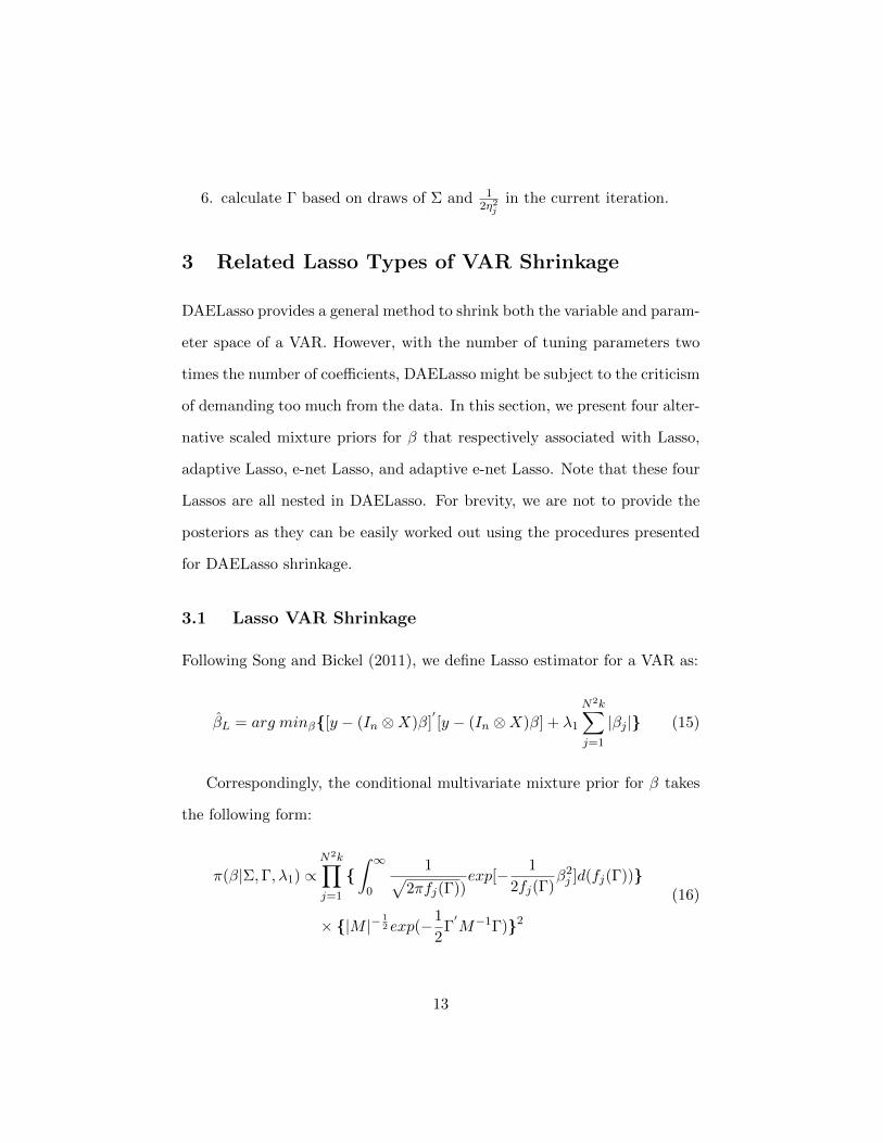
3 Related Lasso Types of VAR Shrinkage

DAELasso provides a general method to shrink both the variable and param-

eter space of a VAR. However, with the number of tuning parameters two

times the number of coefficients, DAELasso might be subject to the criticism

of demanding too much from the data. In this section, we present four alter-

native scaled mixture priors for β that respectively associated with Lasso,

adaptive Lasso, e-net Lasso, and adaptive e-net Lasso. Note that these four

Lassos are all nested in DAELasso. For brevity, we are not to provide the

posteriors as they can be easily worked out using the procedures presented

for DAELasso shrinkage.

3.1 Lasso VAR Shrinkage

Following Song and Bickel (2011), we define Lasso estimator for a VAR as:

βL = arg minβ{[y − (In ⊗X)β]′[y − (In ⊗X)β] + λ1

N2k∑j=1

|βj |} (15)

Correspondingly, the conditional multivariate mixture prior for β takes

the following form:

π(β|Σ,Γ, λ1) ∝N2k∏j=1

{∫ ∞

0

1√2πfj(Γ))

exp[− 1


× {|M |−12 exp(−1

2Γ′M−1Γ)}2

(16)

13

Let fj(Γ) = 2(η2j ), the scale mixture prior is:

π(β|Σ,Γ, λ1) ∝N2k∏j=1

{∫ ∞

0

1√2π(2η2

j ))exp[−

β2j

2(2η2j )

]d(2η2j )

× λ21

2σ2γj

exp[−1

2

2η2j

(σ2γj )/λ

21

]}

(17)

where ηj = τj/λ1.

3.2 Adaptive Lasso VAR Shrinkage

We define the adaptive Lasso estimator for a VAR as:

βAL = arg minβ{[y − (In ⊗X)β]′[y − (In ⊗X)β] +

N2k∑j=1

λ1,j |βj |} (18)


the following form:

π(β|Σ,Γ,Λ1) ∝N2k∏j=1

{∫ ∞

0

1√2πfj(Γ))

exp[− 1


× {|M |−12 exp(−1

2Γ′M−1Γ)}2

(19)


π(β|Σ,Γ,Λ1) ∝N2k∏j=1

{∫ ∞

0

1√2π(2η2

j ))exp[−

β2j

2(2η2j )

]d(2η2j )

×λ2

1,j

2σ2γj

exp[−1

2

2η2j

(σ2γj )/λ

21,j

]}

(20)

14

where ηj = τj/λ1,j .

3.3 E-net Lasso VAR Shrinkage

We define the e-net Lasso estimator for a VAR as:

βEL = arg minβ{[y − (In ⊗X)β]′[y − (In ⊗X)β] + λ1

N2k∑j=1

|βj |+ λ2

N2k∑j=1

β2j }

(21)


the following form:

π(β|Σ,Γ, λ1, λ2) ∝N2k∏j=1

{√λ2√2πexp(−λ2

2β2j )

×∫ ∞

0

1√2πfj(Γ))

exp[− 1


× {|M |−12 exp(−1

2Γ′M−1Γ)}2

(22)


π(β|Σ,Γ, λ1, λ2) ∝N2k∏j=1


2β2j )

×∫ ∞

0

1√2π(2η2

j ))exp[−

β2j

2(2η2j )

]d(2η2j )

× λ21

2σ2γj

exp[−1

2

2η2j

(σ2γj )/λ

21

]}

(23)

where ηj = τj/λ1.

15

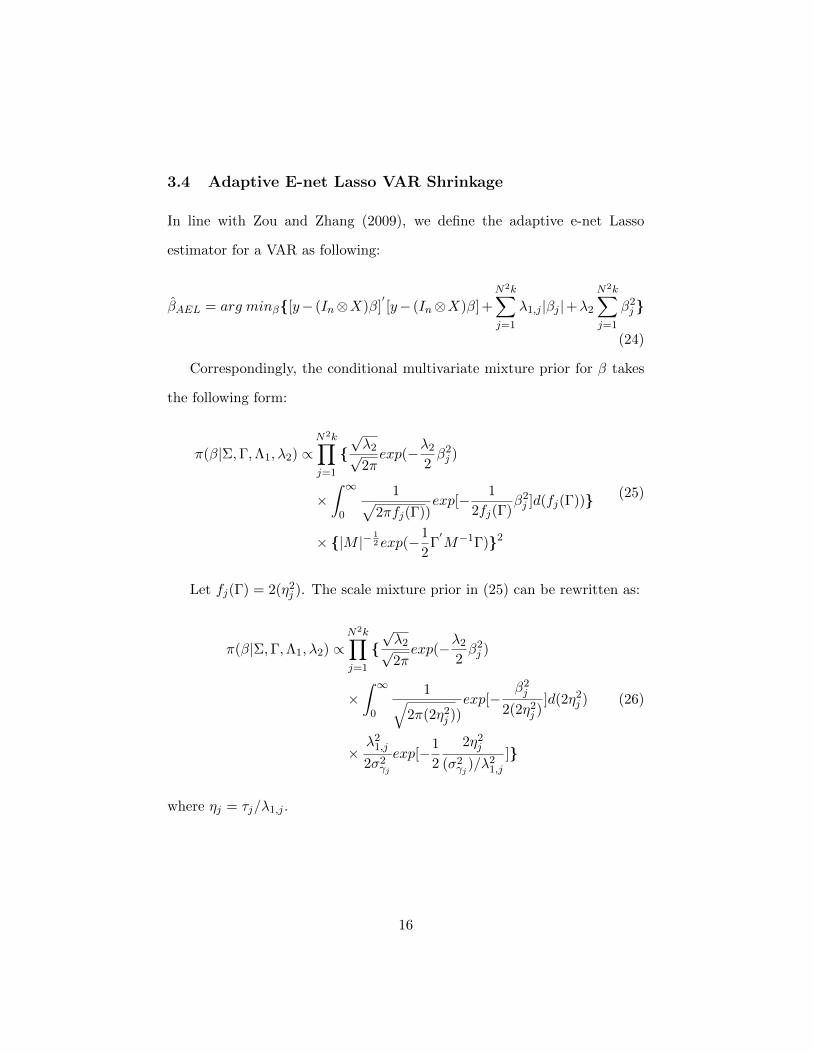
3.4 Adaptive E-net Lasso VAR Shrinkage

In line with Zou and Zhang (2009), we define the adaptive e-net Lasso

estimator for a VAR as following:

βAEL = arg minβ{[y− (In⊗X)β]′[y− (In⊗X)β]+

N2k∑j=1

λ1,j |βj |+λ2

N2k∑j=1

β2j }

(24)


the following form:

π(β|Σ,Γ,Λ1, λ2) ∝N2k∏j=1


2β2j )

×∫ ∞

0

1√2πfj(Γ))

exp[− 1


× {|M |−12 exp(−1

2Γ′M−1Γ)}2

(25)

Let fj(Γ) = 2(η2j ). The scale mixture prior in (25) can be rewritten as:

π(β|Σ,Γ,Λ1, λ2) ∝N2k∏j=1


2β2j )

×∫ ∞

0

1√2π(2η2

j ))exp[−

β2j

2(2η2j )

]d(2η2j )

×λ2

1,j

2σ2γj

exp[−1

2

2η2j

(σ2γj )/λ

21,j

]}

(26)

where ηj = τj/λ1,j .

16

4 Empirical Illustration

4.1 Data

In macroeconomics, it is a standard practice to assess models by their fore-

casting performance (e.g. Litterman, 1986; Giannone et al, 2010). Koop

(2011) provides an extensive forecasts evaluation for seven popular Bayesian

VAR priors. We employ the data set of Koop (2011), an updated version

of that used in Stock and Watson (2008), for the out-of sample forecasting

analysis. The data set contains twenty quarterly macroeconomic series in-

cluding a measure of economic activity (GDP, real GDP), prices (CPI, the

consumer price index), an interest rate (FFR, the Fed funds rate), and other

seventeen variables.3 Four of the seventeen variables are those used in the

monetary model of Christiano el al (1999). The rest of the thirteen variables

contain important aggregated information of the economy. The time series

span from 1959Q1 to 2008Q4. A full list of the variables is provided in the

Appendix. Detailed data descriptions please refer to Koop (2011) and Stock

and Watson (2008). Data are transformed to stationarity and standardized

same as Koop (2011).4

3These 20 variables are used for medium-size VAR in Koop (2011). Koop (2011) alsoexamines the VAR forecasts using medium-large VAR, which contains 40 variables, andlarge VAR, which contains 168 variables. We only focus on Koop’s (2011) medium-sizeVAR in this paper due to two considerations. First, it is computationally costly to useDAELasso priors to estimate the medium-large and large VARs. Second, it is shown inthe literature (e.g. Banbura et al, 2010; Koop, 2011) that most of the gains in forecastingperformance are achieved by using medium VARs of about 20 key variables.

4I am grateful to Mark Watson for providing the data. In addition, I am grateful toGary Koop for sharing the Matlab code for data transformation.

17

4.2 Forecast Evaluation

Same as Koop (2011), we conduct rolling and recursive forecast exercises

and calculate both the mean squared forecast error (MSFE) and predictive

likelihood measures using reduced form VAR of order four. The window

length for the rolling estimation is set to be ten years. Recursive and rolling

forecasts are conducted for t0+h, t0+1+h,...T , where t0 is 1969Q4. Let yft+h

be the hth period forecast of y using data available at time t, and yt+h be the

real value for y observed at t+ h. The MSFE measure for the variable yi is

calculated as an average of the mean squared errors of the point estimates:

MSFE =

∑T−ht=t0

[yi,t+h − E(yfi,t+h|Datat)]2

T − h− t0 + 1(27)

The predictive likelihood is used to evaluate the entire predictive distribu-

tion. In particular, the following sum of the log predictive likelihood is used:

T−h∑t=t0

log[p(yfi,t+h = yi,t+h|Datat)] (28)

For DAELasso, we need to elicit priors for λ21,j , λ2,j , and Σ. It is prac-

tically impossible to set informative priors for each λ21,j and λ2,j , thus we

set relatively uninformative priors for λ21,j and λ2,j to be G(1, 0.001) and

G(1, 0.01), respectively. The prior for Σ−1 is set to be W ( 1N−1IN , 1), which

is also relatively uninformative. There is room for improving the forecasting

performance of DAELasso, in particular by eliciting more informative priors.

We do not explore this possibility in the current paper because the goal of

our exercise is to find out whether a DAELasso with relatively uninforma-

18

tive priors can provide acceptable forecasting results. For comparison, the

priors for Lasso, adaptive Lasso, e-net Lasso, and adaptive e-net Lasso are

set in the same manner.

Tables 1-4 report the DAELasso forecasts results along with Lasso, adap-

tive Lasso, e-net Lasso, adaptive e-net Lasso, and those of the seven pop-

ular Bayesian shrinkage priors in Koop (2011). In line with Koop (2011),

we present MSFE relative to the random walk and log predictive likelihood

for GDP, CPI and FFR. The results for DAELasso and four other Lasso

types of shrinkage methods are reported at the top of each table, followed

by those of the methods reported in Koop (2011). Koop (2011) considers

three variants of the Minnesota prior. The first is the natural conjugate

prior used in Banbura et al (2010), which is labelled ‘Minn. Prior as in

BGR’. The second is the traditional Minnesota prior of Litterman (1986),

which is labelled ‘Minn. Prior Σ diagonal’. The third is the traditional

Minnesota prior except that the upper left 3× 3 block of Σ is not assumed

to be daigonal, which is labelled ‘Minn. Prior Σ not diagonal’. Koop (2011)

also evaluates the performances of four types of SSVS priors. The first is

the same as George et al (2008), which is labelled ‘SSVS Non-conj. semi-

automatic’. The second is a combination of the non-conjugate SSVS prior

and Minnesota prior with variables selected in a data based fashion, which

is labelled ‘SSVS Non-conj. plus Minn. Prior’. The Third is a conjugate

SSVS prior, which is labelled ‘SSVS Conjugate Semi-automatic’. The fourth

is a combination of the conjugate SSVS prior and Minnesota prior, which is

labelled ‘SSVS Conjugate plus Minn. Prior’. We refer to Koop (2011) for a

lucid description of these priors.

19

Table 1: Rolling Forecasting for h = 1

GDP CPI FFR

DAELasso0.5774 0.3172 0.5730

( -198.88 ) ( -192.66 ) ( -211.66 )

adaptive e-net Lasso0.6739 0.3976 0.6312

( -195.78 ) ( -199.37 ) ( -215.03 )

e-net Lasso0.6751 0.3994 0.6326

( -215.29 ) ( -211.6 ) ( -223.72 )

adaptive Lasso0.7663 0.3076 0.6184

( -225.56 ) ( -209.24 ) ( -228.28 )

Lasso0.6697 0.3918 0.6263

( -255.82 ) ( -241.26 ) ( -257.64 )

Minn. Prior as in BGR0.5842 -0.3414 0.5071

( -190.51 ) ( -209.19 ) ( -177.41 )

Minn. Prior Σ diagonal0.6112 0.3048 0.5228

( -194.04 ) ( -193.00 ) ( -181.74 )

Minn. Prior Σ not diagonal0.6092 0.3068 0.526

( -192.12 ) ( -202.38 ) ( -185.88 )

SSVS Conjugate semi-automatic0.8061 0.3808 0.6324

( -209.44 ) ( -231.81 ) ( -175.82 )

SSVS Conjugate plus Minn. Prior0.5916 0.3516 0.5069

( -191.41 ) ( -212.11 ) ( -179.18 )

SSVS Non-conj. semi-automatic0.8780 0.4674 0.7348

( -234.25 ) ( -235.98 ) ( -213.03 )

SSVS Non-conj. plus Minn. Prior0.6766 0.3402 0.5239

( -197.85 ) ( -195.22 ) ( -177.18 )

Notes:

MSFEs as proportion of random walk MSFEs.

Sum of log predictive likelihoods in parentheses.

20

Table 2: Rolling Forecasting for h = 4

GDP CPI FFR

DAELasso0.5545 0.4798 0.6458

( -206.92 ) ( -205.93 ) ( -230.87 )


( -195.68 ) ( -204.38 ) ( -219.92 )

e-net Lasso0.5288 0.4749 0.5494

( -215.24 ) ( -213.47 ) ( -225.49 )

adaptive Lasso0.7428 0.5411 0.7776

( -233.92 ) ( -223.04 ) ( -247.68 )

Lasso0.5286 0.4739 0.5511

( -255.88 ) ( -242.64 ) ( -258.96 )

Minn. Prior as in BGR0.5852 0.5484 0.5847

( -217.08 ) ( -227.69 ) ( -213.38 )


( -211.06 ) ( -232.37 ) ( -246.61 )


( -210.55 ) ( -222.21 ) ( -212.12 )


( -282.63 ) ( -284.27 ) ( -273.83 )


( -230.23 ) ( -221.23 ) ( -213.5 )


( -294.11 ) ( -266.18 ) ( -268.75 )


( -209.89 ) ( -201.3 ) ( -198.07 )

Notes:



21

Table 3: Recursive Forecasting for h = 1

GDP CPI FFR

DAELasso0.5521 0.2882 0.5642

( -210.43 ) ( -190.91 ) ( -224.24 )


( -241.99 ) ( -201.55 ) ( -239.81 )

e-net Lasso0.675 0.3993 0.6325

( -225.62 ) ( -212.49 ) ( -237.91 )

adaptive Lasso0.6248 0.275 0.5965

( -219.17 ) ( -196.36 ) ( -226.84 )

Lasso0.6684 0.3886 0.6245

( -236.48 ) ( -221.09 ) ( -242.93 )


( -192.29 ) ( -195.9 ) ( -229.14 )


( -204.84 ) ( -182.18 ) ( -238.79 )


( -195.4 ) ( -184.06 ) ( -249.09 )


( -199.9 ) ( -191.15 ) ( -245.25 )


( -192.53 ) ( -197.64 ) ( -228.54 )


( -205.12 ) ( -196.47 ) ( -237.16 )


( -203.92 ) ( -187.58 ) ( -228.86 )

Notes:



22

Table 4: Recursive Forecasting for h = 4

GDP CPI FFR

DAELasso0.5434 0.4789 0.6136

( -218.34 ) ( -206.60 ) ( -239.62 )


( -215.61 ) ( -207.02 ) ( -247.3 )

e-net Lasso0.5288 0.4749 0.5494

( -225.54 ) ( -213.7 ) ( -238.98 )

adaptive Lasso0.6297 0.5165 0.664

( -227.95 ) ( -214.7 ) ( -242.16 )

Lasso0.5288 0.4731 0.5496

( -236.24 ) ( -222.75 ) ( -244.27 )


( -214.71 ) ( -219.35 ) ( -249.63 )


( -214.02 ) ( -217.6 ) ( -278.11 )


( -213.28 ) ( -216.07 ) ( -244.77 )


( -212.35 ) ( -225.02 ) ( -249.46 )


( -219.64 ) ( -246.64 ) ( -258.47 )


( -293.21 ) ( -226.36 ) ( -268.06 )


( -219.01 ) ( -201.62 ) ( -233.67 )

Notes:



23

Results presented in Tables 1-4 show that the forecasting performance

of DAELasso approach is comparable to that of the seven popular Bayesian

shrinkage methods explored in Koop (2011). Compared to the results re-

ported in Koop (2011), DAELasso tends to forecast better for GDP and

CPI in terms of point forecasts. In particular DAELasso provides the best

rolling and recursive GDP and CPI point forecasts for h = 4. By contrast,

DAELasso’s point forecasts for FFR are not as good. However, the results

are not too bad as DAELasso’s performance generally ranks in the middle.

The results for predictive loglikelihood yielded by DAELasso approach are

more mixed. Yet, DAELasso’s performances are qualitatively similar to that

of the Bayesian VAR methods studied in Koop (2011).

When we focus on the five Lasso types of forecasts, we find for h = 1,

DAELasso tends to provide the best GDP and FFR point forecasts while

adaptive Lasso gives the best CPI point forecasts. This results seem to

suggest that while GDP and FFR can be better forecasted by using many

variables that might be highly collinear, CPI can be better forecasted using

a smaller number of important variables that are not highly correlated with

each other. Turning to the point forecasts for h = 4, we find more parsi-

monious models such as Lasso are performing better in most of the cases.

This is in consistent with the general notion that parsimonious models are

more valuable when the forecasting horizon gets longer. Forecasts results

for predictive loglikelihood varies for the five Lasso types of methods. But

overall, DAELasso and adaptive e-net Lasso tend to outperform the rest

methods in most of the cases. This result suggest the importance of using

e-net to capture the possible grouping effect, and using different degree of

24

shrinkages for different coefficients.

5 Conclusion

This paper proposes a Bayesian DAELasso approach for VAR shrinkage.

We elicit a scale mixture prior which leads to closed-form posteriors that

can be directly drawn from a Gibbs sampler. The method is appealing as it

can simultaneously achieve variable selection and coefficient shrinkage in a

data based fashion. DAELasso can constructively deal with multicollinearity

problem by encouraging the grouping effect through e-net. In addition, it

achieves adaption through allowing for different degree of shrinkages for

different coefficients. Using relatively uninformative prior, we find that the

forecasting performance of DAELasso is comparable to that of other popular

Bayesian VAR shrinkage methods. This shows that DAELasso approach can

be used as an appropriate addition to the available Bayesian VAR toolkits.

The implementation of DAELasso approach is simple and straightforward.

It can be easily extended into nonlinear framework to shed new light on

macro economic analysis and forecasting.

References

[1] Anderson, T. W. (2003), An introduction to multivariate statistical

analysis, 3rd Ed. John Wiley and Sons: New Jersey.

[2] Andrews, D. F. and C. L. Mallows (1974), Scale mixtures of Normal

distributions, Journal of the Royal Statistical Society, B 36, 99-102.

25

[3] Banbura, M, D. Giannone and L. Reichlin (2010), Large Bayesian vector

auto regressions, Journal of Applied Econometrics, 25, 71-92.

[4] Burns, A. F and W. C. Mitchell (1946), Measuring Business Cycles,

New York: NBER.

[5] Christiano, L. J., M. Eichenbaum and C. L. Evans (1999), Monetary

policy shocks: what have we learned and to what end? in Taylor J.

B. and M. Woodford (eds) Handbook of Macroeconomics 1, 65-148,

Elsevier: Amsterdam.

[6] Chudik, A. and Pesaran, M. H. (2011), Infinite dimensional VARs and

factor models, Journal of Econometrics, 163, 1, 4-22.

[7] De Mol, C., Giannone, D. and Reichlin, L. (2008), Forecasting using a

large number of predictors: is Bayesian shrinkage a valid alternative to

principal components? Journal of Econometrics, 146, 318-28.

[8] Doan, T., R. Litterman and C. Sims (1984), Forecasting and conditional

projections using realistic prior distributions, Econometric Reviews, 3,

1-100.

[9] Eltoft, T., T. Kim, and T. Lee (2006), On the multivariate Laplace

distribution, IEEE Signal Proc. Let. 13 (5), 300-3.

[10] George, E. and R. McCulloch (1993), Variable selection via Gibbs sam-

pling, Journal of the American Statistical Association, 88, 881-89.

[11] George, E. and R. McCulloch (1997), Approaches for Bayesian variable

selection, Statist. Sinica, 7, 339-73.

26

[12] George, E., D. Sun and S. Ni (2008), Bayesian stochastic search for

VAR model restrictions, Journal of Econometrics, 142, 553-80.

[13] Giannone, M., M. Lenza and G. Primiceri (2010), Prior selection for

vector autoregressions, Working paper, Universite Libre de Bruxelles.

[14] Griffin, J. E. and P. J. Brown (2010), Bayesian adaptive lassos with non-

convex penalization, Australian and New Zealand Journal of Statistics,

forthcoming.

[15] Kadiyala, K.R. and S. Karlsson (1997), Numerical methods for estima-

tion and inference in Bayesian VAR-models, Journal of Applied Econo-

metrics, 12(2), 99-132.

[16] Koop, G. (2003), Bayesian econometrics, John Wiley and Sons: Chich-

ester.

[17] Koop, G. (2011), Forecasting with medium and large Bayesian VARs,

Journal of Applied Econometrics, doi: 10.1002/jae.1270.

[18] Korobilis, D. (2011), Hierarchical shrinkage priors for dynamic regres-

sions with many predictors, MPRA Paper No. 30380.

[19] Kotz, S., T. J. Kozubowski and K. Podgorski (2001), The Laplace dis-

tribution and generalizations: a revisit with applications to communi-

cations, economics, engineering, and finance, Birkhauser Boston.

[20] Kwon, D.W., Landi, M.T., Vannucci, M., Issaq, H.J., Prieto, D. and

Pfeiffer, R.M. (2011), An efficient stochastic search for Bayesian vari-

27

able selection with high-dimensional correlated predictors, Computa-

tional Statistics and Data Analysis, 55(10), 2807-18.

[21] Kyung, M., J. Gill, M. Ghosh, and G. Casella (2010), Penalized Re-

gression, Standard Errors, and Bayesian Lassos, Bayesian Analysis, 5,

369-412.

[22] Leng, C, M. N. Tran and D. Nott (2010), Bayesian adaptive Lasso,

arXiv:1009.2300v1

[23] Litterman, R.(1986), Forecasting with Bayesian vector autoregressions

five years of experience, Journal of Business and Economics Statistics,

4, 25-38.

[24] Muirhead R. J. (1982), Aspects of Multivariate Statistical Theory, Wi-

ley: New York.

[25] Park, T. and G. Casella (2008), The Bayesian Lasso, Journal of the

American Statistical Association, 103, 681-86.

[26] Sims, C. (1972), Money, Income and Causality, American Economic

Review, 62, 540-52.

[27] Sims, C. (1980), Macroeconomics and Reality, Econometrica, 48, 1-48.

[28] Song, S. and P. Bickel (2010), Large vector auto regressions,

arXiv:1106.3915v1.

[29] Stock, J. H. and M. W. Watson (1989), New Indexes of Coincident and

Leading Economic Indicators, NBER Macroeconomic Annual , 351-94.

28

[30] Stock, J. H. and M. W. Watson (2008), Forecasting in dynamic factor

models subject to structural instability, in Castle, J. and N. Shephard

(eds) The Methodology and Practice of Econometrics: A Festschrift in

Honour of Professor David F. Hendry, 173205. Oxford University Press:

Oxford.

[31] Tibshirani, R. (1996), Regression shrinkage and selection via the Lasso,

Journal of the Royal Statistical Society, B 58, 267-88.

[32] van Gerven, M., B. Cseke, R. Oostenveld and T. Heskes (2009),

Bayesian Source Localization with the Multivariate Laplace Prior, in Y.

Bengio, D. Schuurmans, J. Lafferty, C. K. I. Williams and A. Culotta

(eds.) Advances in Neural Information Processing Systems 22, 1901-09.

[33] van Gerven, M., B. Cseke, F. P. de Lange and T. Heskes (2010), Efficient

Bayesian multivariate fMRI analysis using a sparsifying spatio-temporal

prior, NeuroImage, 50, 150-61.

[34] Yuan, M. and Y. Lin (2007), Model selection and estimation in regres-

sion with grouped variables, Journal of the Royal Statistical Society, B

68(1), 49-67.

[35] Zellner, A. (1971). An introduction to Bayesian inference in economet-

rics, John Wiley and Sons: New York.

[36] Zou, H. (2006), The adaptive Lasso and its oracle properties, Journal

of the American Statistical Association, 101, 1418-29

29

[37] Zou, H. and T. Hastie (2005), Regularization and variable selection via

the elastic net, Journal of the Royal Statistical Society, B 67, 301-20.

[38] Zou, H. and Zhang, H. H. (2009), On the adaptive elastic-Net with a

diverging number of parameters, Ann. Statist., 37, 1733-51.

30

Appendix: Data List

We use 20 US macro series used in Koop (2011), which is an updated

version of Stock and Watson (2008). The variables are transformed to sta-

tionarity and standardized same as Koop (2011). Below we cite the essential

data description and transformation code from Koop (2011). Please refer to

Koop (2011) for detailed data information.

The data transformation codes are as following: 1: no transformation;

2: first difference; 3: second difference; 4: log; 5: first difference of logged

variables; 6: second difference of logged variables.

Table 5: The List of Variables

Short name Trans. Code Data DescriptionRGDP 5 Real GDP, quantity index (2000 = 100)CPI 6 CPI all itemsFFR 2 Interest rate: federal funds (e-ective) (% per annum)Com: spot price (real) 5 Real spot market price index: all commoditiesReserves nonbor 3 Depository inst reserves: nonborrowed (mil$)Reserves tot 6 Depository inst reserves: total (mil$)M2 6 Money stock: M2 (bil$)Cons 5 Real Personal Cons. Exp., Quantity IndexIP: total 5 Industrial production index: totalCapacity Util 1 Capacity utilization: manufacturing (SIC)U: all 2 Unemp. rate: All workers, 16 and over (%)HStarts: Total 4 Housing starts: Total (thousands)PPI: fin gds 6 Producer price index: finished goodsPCED 6 Personal Consumption Exp.: price indexReal AHE: goods 5 Real avg hrly earnings, non-farm prod. workerM1 6 Money stock: M1 (bil$)S&P: indust 5 S&Ps common stock price index: industrials10 yr T-bond 2 Interest rate: US treasury const. mat., 10-yrEx rate: avg 5 US effective exchange rate: index numberEmp: total 5 Employees, nonfarm: total private

31

bayesian doubly adaptive elastic-net lasso for var shrinkage

Documents