bayesian evidence and model...

Bayesian Evidence and Model Selection: A Tutorial in Two Acts

Kevin H. Knuth Depts. of Physics and Informatics, University at Albany, Albany NY USA Based on the paper: Knuth K.H., Habeck M., Malakar N.K., Mubeen A.M., Placek B. 2015. Bayesian evidence and model selection. In press at Digital Signal Processing. doi:10.1016/j.dsp.2015.06.012

DOWNLOAD TALK NOW: Google ‘knuthlab’ Click ‘Talks’

7/19/2015 MaxEnt 2015 Tutorial 1

http://dx.doi.org/10.1016/j.dsp.2015.06.012


This tutorial follows the paper: Knuth K.H., Habeck M., Malakar N.K., Mubeen A.M., Placek B. 2015. Bayesian evidence and model selection. In press at Digital Signal Processing. doi:10.1016/j.dsp.2015.06.012

References are not provided in the talk slides, please consult the paper Equations in the talk are numbered in accordance with the paper When referencing anything from Act 1 of this talk, please reference this paper When referencing anything from Act 2 of this talk, please reference the slides

http://dx.doi.org/10.1016/j.dsp.2015.06.012


Bayesian Evidence Odds Ratios Evidence, Model Order and Priors Numerical Techniques Laplace Approximation Importance Sampling Annealed Importance Sampling Variational Bayes Nested Sampling

Applications Signal Detection : Brain Computer Interface / Neuroscience Sensor Characterization : Robotics / Signal Processing Exoplanet Characterization : Astronomy / Astrophysics Examples Nested Sampling Demo Nested Sampling and Phase Transitions


Bayesian Evidence


Bayesian Evidence : Odds Ratios : oooo

Bayes Theorem

M represents a class of models represented by a set of model parameters m represents a particular model defined by a set of particular model parameter values d represents the acquired data

Posterior Probability Likelihood Prior Probability

Evidence or Marginal Likelihood



Bayesian Evidence The Bayesian evidence can be found by marginalizing the joint distribution 𝑃 𝑚, 𝑑|𝑀, 𝐼 over all model parameter values.

M represents a class of models represented by a set of model parameters m represents a particular model defined by a set of particular model parameter values d represents the acquired data I represents the dependence on any relevant prior information



Model Comparison We derive the ratio of probabilities of two models given data

If the prior probabilities of the models are equal then this is the ratio of evidences



Odds Ratio or Bayes Factor

The ratio of probabilities of the models given the data is proportional to the Odds Ratio


Bayesian Evidence : Evidence, Model Order and Priors : ooooo

Evidence: Model Order and Priors It is instructive to see how the evidence depends on both the model order and prior probabilities Consider a model with a single parameter: 𝑥 𝜖 [𝑥𝑚𝑖𝑛, 𝑥𝑚𝑎𝑥] with a width of ∆𝑥 = 𝑥𝑚𝑎𝑥 − 𝑥𝑚𝑖𝑛 Define the effective width

where 𝐿𝑚𝑎𝑥 is the maximum likelihood value.



Model with a Single Parameter Consider a model with a single parameter: 𝑥 𝜖 [𝑥𝑚𝑖𝑛, 𝑥𝑚𝑎𝑥] with a width of ∆𝑥 = 𝑥𝑚𝑎𝑥 − 𝑥𝑚𝑖𝑛 Given the effective width

The evidence is



Occam Factor The evidence is proportional to the ratio of the effective width of the likelihood and the width of the prior

This ratio 𝛿𝑥

∆𝑥 is called the Occam factor after Occam’s Razor:

"Non sunt multiplicanda entia sine necessitate", " Entities must not be multiplied beyond necessity “

- William of Ockham



Model Order For models with multiple parameters this generalizes to the ratio of the volume of the models that are compatible with both the data and the prior and the prior volume. If we assume that each of the 𝐾 parameters has prior width ∆𝑥

then the Occam factor scales as 𝛿𝑥

∆𝑥

𝐾. As model parameters

added, eventually one fits the data asymptotically well so that 𝛿𝑥 attains a maximum value and further model parameters can only decrease the Occam factor. If we increase the flexibility of our model by the introduction of more model parameters, we reduce the Occam factor.



Odds Ratios and Occam Factors We compute the odds ratio for a model 𝑀0 without model parameters to a model 𝑀1 with a single model parameter.

𝐿𝑚𝑎𝑥 ratio Occam Factor

The likelihood ratio is a classical statistic in frequentist model selection. If we only consider the likelihood ratio in model comparison problems, we fail to acknowledge the importance of Occam factors.


Numerical Techniques


Numerical Techniques : o

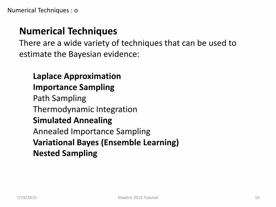
Numerical Techniques There are a wide variety of techniques that can be used to estimate the Bayesian evidence:

Laplace Approximation Importance Sampling Path Sampling Thermodynamic Integration Simulated Annealing Annealed Importance Sampling Variational Bayes (Ensemble Learning) Nested Sampling


Numerical Techniques : Laplace Approximation : oooo

Laplace Approximation is a simple and useful method for approximating a unimodal probability density function with a Gaussian Consider a function 𝑝 𝑥 with a peak at 𝑥 = 𝑥0 We write a Taylor series expansion of ln 𝑝 𝑥 about 𝑥 = 𝑥0

which can be simplified to



Laplace Approximation

By defining

We can write

Previously, we had




By taking the exponential we can approximate the density by

with an integral (evidence) of:

Previously, we had




The evidence is then

In the case of a multidimensional posterior we have

where


Numerical Techniques : Importance Sampling : oooo

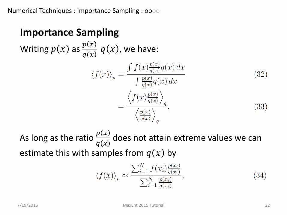
Importance Sampling allows one to find expectation values with respect to one distribution p(x) by computing expectation values with respect to a second distribution q(x) that is easier to sample from.

The expectation value of 𝑓 𝑥 with respect to 𝑝 𝑥 is given by

One can write 𝑝 𝑥 as 𝑝 𝑥

𝑞 𝑥 𝑞 𝑥 as long as 𝑞 𝑥 is non-zero

whenever 𝑝 𝑥 is nonzero.



Importance Sampling

Writing 𝑝 𝑥 as 𝑝 𝑥

𝑞 𝑥 𝑞 𝑥 , we have:

As long as the ratio 𝑝 𝑥

𝑞 𝑥 does not attain extreme values we can

estimate this with samples from 𝑞 𝑥 by



Importance Sampling Importance sampling can be used to compute ratios of evidence values in a similar fashion by writing



Importance Sampling The evidence ratio can be found by sampling from 𝑞 𝑥 as long as

𝑝 𝑥 is sufficiently close to 𝑞 𝑥 to avoid extreme ratios of 𝑝 𝑥

𝑞 𝑥


Numerical Techniques : Variational Bayes : ooo

Variational Bayes which is also known as ensemble learning, relies on approximating The posterior 𝑃 𝑚|𝑀, 𝐼 with another distribution 𝑄 𝑚 .

By defining the negative Free Energy

And the Kullback-Leibler (KL) Divergence

We can write



Variational Bayes With this expression in hand

We can show that the negative Free Energy is a lower bound to the evidence

By minimizing the negative Free Energy, we can approximate the evidence



Variational Bayes By choosing a distribution 𝑄 𝑚 that factorizes into

where

where the set of parameters 𝑚0 is disjoint from 𝑚1we can minimize the negative Free Energy and estimate the evidence by choosing


Numerical Techniques : Nested Sampling : ooooooo

Nested Sampling was developed by John Skilling to stochastically integrate the posterior probability to obtain the evidence. Posterior estimates are used to obtain model parameter estimates. Nested sampling aims to estimate the cumulative distribution function of the density or states (DOS), which is the prior probability mass enclosed within a likelihood boundary.



Nested Sampling Given a likelihood 𝐿, one can find the prior mass such that the likelihood of those states is greater than 𝐿

Parameter Space



Nested Sampling One can then estimate the evidence via stochastic integration using samples distributed according to the prior

Likelihood integrated over Prior



Nested Sampling One begins with a set of N samples. Use the sample with the lowest likelihood to define an implicit likelihood boundary. This results in an average decrease of the prior volume by 1/N Sample from the prior (uniformly is easiest) from within the implicit likelihood boundary to maintain N samples Keep track of 𝐿𝑖 (𝑋𝑖+1 − 𝑋𝑖)𝑖 to estimate the evidence Z



Nested Sampling Note how the prior volume contracts by 1/N each time. Early steps contribute little to the integral (𝑍) since the likelihood is very low. Later steps contribute little to (𝑍) since the prior volume change is very small. The steps that contribute most are in the middle of the sequence.



Nested Sampling Since nested sampling contracts along the prior volume, it is relatively unaffected by local maxima in evidence (phase transitions). (See Figure A) Methods based on tempering, such as simulated annealing follow the slope of the log L curve and as such, get stuck at phase transitions. (See Figure B)



Nested Sampling The great challenge is sampling uniformly (from the prior) within the implicit Likelihood boundaries. Several versions of Nested Sampling now exist: MultiNest (developed by Feroz and Hobson): clusters samples (K-means) and fits clusters with ellipsoids. Samples uniformly from within those ellipsoids. Very fast. Excellent performance for multi-modal distributions. Clustering limits this to 10s of parameters and the ellipsoids may not cover the high likelihood regions. Galilean Monte Carlo (Developed by Feroz and Skilling): moves a new sample with momentum reflecting off of logL boundaries. Excellent at handling ridges both angled and curved. Constrained Hamilton Monte Carlo (developed by M. Betancourt): similar to Galilean Monte Carlo. Diffusive Nested Sampling (developed by Brewer): allows samples to diffuse to lower likelihood nested levels and takes a weighted average. Nested Sampling with Demons (developed by M. Habeck): utilizes “demon variables” that smooth the constraint boundary and push the samples away from it.


Signal Detection Brain Computer Interface / Neuroscience

Applications: Signal Detection: oooooooo


Signal Detection (Mubeen and Knuth)

We consider a practical signal detection problem where the log odds-ratio can be analytically derived. The specific application was originally for the detection of evoked brain responses


The signal absent case models the recording 𝑥 in channel 𝑚 as noise

The signal present case models the recording 𝑥 in channel 𝑚 as signal plus where the signal has a amplitude parameter 𝛼 and can be coupled differently to different detectors (via 𝐶)


Considering the Evidence


The odds ratio can be written as

For the noise only case, the evidence is the likelihood (Gaussian)




In the signal plus noise case, the evidence is

Assigning a Gaussian Likelihood and Prior for 𝛼




We can then write the evidence as

where




If the signal amplitude must be positive: 𝛼 𝜖 0, +∞ then:

If amplitude can be positive or negative: 𝛼 𝜖 −∞,+∞ then:




Look at:

The expression E (86) contains the cross-correlation term, which is what is typically used for the detection of a target signal in ongoing recordings. The log OR detection filters incorporate more information that leads to extra terms, which serve to aid in target signal detection.


Detecting Signals


A. The P300 template target signal. B. An example of three channels (Cz, Pz, Fz) of synthetic ongoing EEG with two P300 target signal events (indicated by the arrows) at an SNR of 5 dB.


Signal Detection Performance


Detection performance measured by that area under the ROC curve as a function of signal SNR. Both OR techniques outperform cross-correlation!


Sensor Characterization Robotics / Signal Processing

Applications: Signal Detection: oooo


Modeling a Robotic Sensor (Malakar, Gladkov, Knuth)

In this project, we aim to model the spatial sensitivity function of a LEGO light sensor for use on a robotic system.


Here the application is to develop a robotic arm that can characterize the white circle by measuring light intensities are various locations. By modeling the light sensor, we aim to increase the robot’s performance.


Modeling a Robotic Sensor The LEGO light sensor was slowly moved over a black-and-white albedo pattern on the surface of a table to obtain calibration data. Sensor orientation was varied as well.



Modeling a Robotic Sensor Mixture of Gaussians models were used. Four model orders were tested using Nested Sampling. The 1-MoG model was slightly favored.


Note the increasing uncertainty as the model becomes more complex. This suggests that the permutation space was not fully explored.


Examining the Sensor Model Performance Here we show a comparison between the 1-MoG model and the data



Star System Characterization Astronomy / Astrophysics

Applications: Star System Characterization: ooooooo


Star System Characterization (Placek and Knuth)

In our DSP paper, we give an example of Bayesian model testing applied to exoplanet characterization. Ben Placek also has a paper and poster here at MaxEnt 2015 on the topic. Here I will apply these model testing concepts to determining the orbital configuration of a triple star system.

Digital Sky Survey (DSS)


Photometric data obtained from the Kepler mission (A) Quarter 13 light curve folded on the P1 = 6.45 day period, (B) Quarter 13 light curve folded on the P2 = 0.645 day period (C) is the entire Q13 light curve.

Digital Sky Survey (DSS)

KIC 5436161: Two Periods This star exhibits oscillations of two commensurate periods in its Light curve: 6.45 days and 0.645 days (a rare 10:1 resonance!)



Courtesy of Geoff Marcy and Howard Issacson

KIC 5436161: Radial Velocity Measurements Eleven radial velocity measurements taken over the span of a week. The 6.45 day period is visible, but not the 0.645 day period.



(A) A hierarchical arrangement (C1 and C2 orbit G with 6.45 day period, and orbit one another with 0.645 day period)

(B) A planetary arrangement (C1 orbits with 6.45 day period, and C2 orbits with 0.645 day period)


KIC 5436161: Models Two possible models of the system. The main star is a G-star (like our sun), at least one of the other companions (C1) is M-dwarf.




KIC 5436161: Results Testing the Hierarchical Model against the Planetary Model using the Radial Velocity Data. The Circular Hierarchical Model has the greatest evidence (by a factor of 𝑒𝑥𝑝 3.73 ≈ 42)


KIC 5436161 This system is a hierarchical triple system consisting of a G-star with two co-orbiting M-dwarfs in a 1:10 resonance (P1 = 6.45 day , P2 = 0.645 day)




KIC 5436161


Nested Sampling Demo (sans model testing)

Demonstrations: Nested Sampling: Lighthouse Problem: ooooo


Nested Sampling Demo The Lighthouse Problem (Gull) Consider a Lighthouse located just off of a straight shore that extends a great distance. Imagine that the lighthouse has a laser beam that it fires at random times as it rotates with a uniform speed. Along the shore are light detectors that detect laser beam hits. Based on this data, where is the lighthouse?



The Likelihood Function It is a useful exercise to derive the likelihood

via a change of variables.


𝑝 𝑥|𝐼 = 𝛽

𝜋 𝛽2 + 𝛼 − 𝑥 2

𝑥 = 𝛽 tan 𝜃 + 𝛼

We assign a uniform prior for the location parameters 𝛼 and 𝛽


Nested Sampling Run using D = 64 data points (recorded flashes) and N = 100 samples Iteration is halted when Δ log 𝑍 = 10−7


o Live Samples + Used Samples

# Iterations = 1193 Log Z = -0.401 +- 0.076 mean(x) = 0.48 ± 0.26 mean(y) = 0.51 ± 0.28

x position

y p

osi

tio

n

Location of Lighthouse


Nested Sampling Run This shows the relationship between log L and log Prior Volume



Nested Sampling Run with a Gaussian Likelihood This shows the relationship between log L and log Prior Volume



Nested Sampling and

Phase Transitions

Applications: Nested Sampling and Phase Transitions: oooo


Peaks on Peaks Here is a Gaussian Likelihood with a taller peak on the side



Nested Sampling with Phase Transitions Phase Transitions represent local peaks in the evidence


Phase Transition


Acoustic Source Localization: One Detector Consider an acoustic source localization problem using a single detector. There is a low (red) and a high (blue) frequency source. Note how the high frequency source is found first inducing a phase transition:



Acoustic Source Localization: Two Detectors In this example, we have two detectors, which allow us to localize the sources to rings. Again, the low frequency source is found first.



Acknowledgements Michael Habeck Nabin Malakar Asim Mubeen

Ben Placek

bayesian evidence and model...

Documents