bayesian inference for stochastic kinetic models using ... · bayesian inference for stochastic...
TRANSCRIPT

Bayesian inference for stochastic kinetic
models using data on proportions of cell
death
Holly F. Ainsworth
Thesis submitted for the degree of
Doctor of Philosophy
School of Mathematics & Statistics
Newcastle University
Newcastle upon Tyne
United Kingdom
May 2014

Acknowledgements
I am deeply grateful to my supervisors, Richard Boys and Colin Gillespie. They have
been generous with their time and unwavering with their support. Their enthusiasm
has been infectious throughout and without their assistance, this thesis would never
have been started, nor would it ever have been finished. Thank you.
Discussions with Andy Golightly, Daniel Henderson and Carole Proctor have all
been extremely helpful. Thank you for giving your time and advice so generously.
To my friends and colleagues in the School of Mathematics and Statistics who made
my time there so thoroughly enjoyable – thank you all. Special thanks must go to Nina
and Joy for their friendship and support throughout.
I would also like to express my gratitude to the Engineering and Physical Sciences
Research Council for the financial support which made the writing of this thesis possible,
and to the School of Mathematics and Statistics at Newcastle University who have
provided a supportive and pleasant atmosphere throughout my time here.
I owe a very important debt to Tom for his constant love, patience and kindness
and for being so understanding – I can’t wait for the next chapter! Special thanks must
go my family: Claire, Jules, Steve, Gordon, Ella, Rory, Tom, Phoebe and Rose – thank
you all for the love and laughter. Finally, I would like to thank my Mum and Dad –
your love, kindness and support has helped me more than you will ever know.

Abstract
The PolyQ model is a large stochastic kinetic model that describes protein aggregation
within human cells as they undergo ageing. The presence of protein aggregates in cells
is a known feature in many age-related diseases, such as Huntington’s. Experimental
data are available consisting of the proportions of cell death over time. This thesis is
motivated by the need to make inference for the rate parameters of the PolyQ model.
Ideally observations would be obtained on all chemical species, observed continuously
in time. More realistically, it would be hoped that partial observations were available
on the chemical species observed discretely in time. However, current experimental
techniques only allow noisy observations on the proportions of cell death at a few discrete
time points. This presents an ambitious inference problem.
The model has a large state space and it is not possible to evaluate the data likelihood
analytically. However, realisations from the model can be obtained using a stochastic
simulator such as the Gillespie algorithm. The time evolution of a cell can be repeatedly
simulated, giving an estimate of the proportion of cell death. Various MCMC schemes
can be constructed targeting the posterior distribution of the rate parameters. Although
evaluating the marginal likelihood is challenging, a pseudo-marginal approach can be
used to replace the marginal likelihood with an easy to construct unbiased estimate.
Another alternative which allows for the sampling error in the simulated proportions is
also considered.
Unfortunately, in practice, simulation from the model is too slow to be used in an
MCMC inference scheme. A fast Gaussian process emulator is used to approximate
the simulator. This emulator produces fully probabilistic predictions of the simulator
output and can be embedded into inference schemes for the rate parameters.
The methods developed are illustrated in two smaller models; the birth-death model
and a medium sized model of mitochondrial DNA. Finally, inference on the large PolyQ
model is considered.
Contents
1 Introduction 1
1.1 Overview of thesis . . . . . . . . . . . . . . . . . . . . . . . . . . . . . . 3
2 Stochastic Modelling 6
2.1 Chemical reaction notation . . . . . . . . . . . . . . . . . . . . . . . . . 6
2.2 Markov jump process . . . . . . . . . . . . . . . . . . . . . . . . . . . . . 7
2.2.1 Chemical master equation . . . . . . . . . . . . . . . . . . . . . . 9
2.2.2 The direct method . . . . . . . . . . . . . . . . . . . . . . . . . . 10
2.3 Example: the birth–death model . . . . . . . . . . . . . . . . . . . . . . 11
2.4 Example: mitochondrial DNA model . . . . . . . . . . . . . . . . . . . . 12
2.5 Example: the PolyQ model . . . . . . . . . . . . . . . . . . . . . . . . . 14
2.6 Other simulation strategies . . . . . . . . . . . . . . . . . . . . . . . . . 20
2.6.1 Exact simulation strategies . . . . . . . . . . . . . . . . . . . . . 20
2.6.2 Approximate simulation strategies . . . . . . . . . . . . . . . . . 21
2.6.3 Hybrid simulation strategies . . . . . . . . . . . . . . . . . . . . . 22
3 Bayesian inference 24
3.1 State–space models . . . . . . . . . . . . . . . . . . . . . . . . . . . . . . 24
3.2 Introduction to Bayesian inference . . . . . . . . . . . . . . . . . . . . . 25
3.3 Markov chain Monte Carlo (MCMC) . . . . . . . . . . . . . . . . . . . . 26
3.4 Likelihood free inference . . . . . . . . . . . . . . . . . . . . . . . . . . . 30
3.4.1 Likelihood free MCMC . . . . . . . . . . . . . . . . . . . . . . . . 31
i

Contents
3.4.2 Pseudo–marginal approach . . . . . . . . . . . . . . . . . . . . . 33
3.4.3 Particle filtering . . . . . . . . . . . . . . . . . . . . . . . . . . . 35
3.4.4 Application to pseudo–marginal approach . . . . . . . . . . . . . 38
3.4.5 Algorithm performance . . . . . . . . . . . . . . . . . . . . . . . 39
4 Numerical examples 41
4.1 Constant model . . . . . . . . . . . . . . . . . . . . . . . . . . . . . . . . 41
4.1.1 Constant model (with approximation) . . . . . . . . . . . . . . . 46
4.1.2 Constant model: results . . . . . . . . . . . . . . . . . . . . . . . 50
4.2 Birth–death model . . . . . . . . . . . . . . . . . . . . . . . . . . . . . . 51
4.2.1 Simulating from the model . . . . . . . . . . . . . . . . . . . . . 53
4.2.2 Inference for known extinction times . . . . . . . . . . . . . . . . 55
4.2.3 Inference for discretised extinction times . . . . . . . . . . . . . . 57
4.2.4 Inference for noisy proportions of extinction . . . . . . . . . . . . 59
4.2.5 Exact probability of extinction . . . . . . . . . . . . . . . . . . . 59
4.2.6 Approximate probability of extinction . . . . . . . . . . . . . . . 60
4.2.7 Approaches to inference . . . . . . . . . . . . . . . . . . . . . . . 60
4.2.8 Comparing algorithm performance . . . . . . . . . . . . . . . . . 64
5 Gaussian process emulation 68
5.1 Building an emulator . . . . . . . . . . . . . . . . . . . . . . . . . . . . . 70
5.1.1 Choice of mean function . . . . . . . . . . . . . . . . . . . . . . . 72
5.1.2 Choice of covariance function . . . . . . . . . . . . . . . . . . . . 73
5.1.3 1-D birth–death example . . . . . . . . . . . . . . . . . . . . . . 74
5.1.4 Training data design . . . . . . . . . . . . . . . . . . . . . . . . . 74
5.2 Estimating hyperparameters . . . . . . . . . . . . . . . . . . . . . . . . . 76
5.3 Other approaches to hyperparameter estimation . . . . . . . . . . . . . . 79
5.3.1 Sparse covariance approach . . . . . . . . . . . . . . . . . . . . . 80
5.4 Diagnostics . . . . . . . . . . . . . . . . . . . . . . . . . . . . . . . . . . 82
5.4.1 Individual prediction errors . . . . . . . . . . . . . . . . . . . . . 84
ii

Contents
5.4.2 Mahalanobis distance . . . . . . . . . . . . . . . . . . . . . . . . 85
5.4.3 Probability integral transform . . . . . . . . . . . . . . . . . . . . 85
6 Parameter inference using Gaussian process emulators 87
6.1 Emulator construction . . . . . . . . . . . . . . . . . . . . . . . . . . . . 88
6.1.1 Emulating approximate proportions . . . . . . . . . . . . . . . . 89
6.1.2 Training data design . . . . . . . . . . . . . . . . . . . . . . . . . 91
6.1.3 Choice of mean function . . . . . . . . . . . . . . . . . . . . . . . 92
6.1.4 Choice of covariance function . . . . . . . . . . . . . . . . . . . . 94
6.1.5 Hyperparameter estimation . . . . . . . . . . . . . . . . . . . . . 96
6.1.6 Diagnostics . . . . . . . . . . . . . . . . . . . . . . . . . . . . . . 100
6.2 Inference for model parameters . . . . . . . . . . . . . . . . . . . . . . . 103
6.2.1 Results of inference using emulators . . . . . . . . . . . . . . . . 104
6.2.2 Considering the uncertainty of hyperparameters . . . . . . . . . . 106
6.3 Emulators with sparse covariance matrices . . . . . . . . . . . . . . . . . 108
6.4 Comparing emulators with sparse and non-sparse covariance matrices . 114
6.5 Conclusion . . . . . . . . . . . . . . . . . . . . . . . . . . . . . . . . . . 114
7 Mitochondrial DNA model 116
7.1 A stochastic model . . . . . . . . . . . . . . . . . . . . . . . . . . . . . . 117
7.1.1 Modelling neuron survival . . . . . . . . . . . . . . . . . . . . . . 121
7.2 Emulation for neuron survival . . . . . . . . . . . . . . . . . . . . . . . . 122
7.2.1 Obtaining training data . . . . . . . . . . . . . . . . . . . . . . . 123
7.2.2 Mean and covariance function . . . . . . . . . . . . . . . . . . . . 124
7.2.3 Estimating hyperparameters and diagnostics . . . . . . . . . . . 125
7.3 Analysis of simulated data . . . . . . . . . . . . . . . . . . . . . . . . . . 125
7.4 Analysis of experimental data . . . . . . . . . . . . . . . . . . . . . . . . 129
7.5 Conclusions . . . . . . . . . . . . . . . . . . . . . . . . . . . . . . . . . . 132
iii

Contents
8 PolyQ model 134
8.1 Introduction . . . . . . . . . . . . . . . . . . . . . . . . . . . . . . . . . . 134
8.2 The stochastic model . . . . . . . . . . . . . . . . . . . . . . . . . . . . . 136
8.3 Experimental data . . . . . . . . . . . . . . . . . . . . . . . . . . . . . . 140
8.4 Emulating proportions of death from the PolyQ model . . . . . . . . . . 142
8.4.1 Mean function and covariance function . . . . . . . . . . . . . . . 142
8.4.2 Training data . . . . . . . . . . . . . . . . . . . . . . . . . . . . . 143
8.4.3 Estimating hyperparameters and diagnostics . . . . . . . . . . . 143
8.5 Analysis of simulated data . . . . . . . . . . . . . . . . . . . . . . . . . . 144
8.6 Further considerations . . . . . . . . . . . . . . . . . . . . . . . . . . . . 149
9 Conclusions and future work 151
9.1 Future work . . . . . . . . . . . . . . . . . . . . . . . . . . . . . . . . . . 152
Bibliography 155
iv
List of Algorithms
1 Stochastic simulation: Gillespie’s direct method . . . . . . . . . . . . . . 11
2 Metropolis–Hastings algorithm . . . . . . . . . . . . . . . . . . . . . . . 27
3 Likelihood free MCMC . . . . . . . . . . . . . . . . . . . . . . . . . . . . 33
4 Pseudo–marginal approach . . . . . . . . . . . . . . . . . . . . . . . . . 34
5 Sequential importance resampling (SIR) filter . . . . . . . . . . . . . . . 38
6 Constant model: inference using the vanilla scheme . . . . . . . . . . . . 47
7 Constant model: inference using the pseudo-marginal scheme . . . . . . 48
8 Birth–death model: inference using known extinction times . . . . . . . 56
9 Birth–death model: inference using discretised extinction times . . . . . 58
10 Birth–death model: inference using the vanilla scheme . . . . . . . . . . 61
11 Birth–death model: inference using pseudo-marginal scheme 1 . . . . . . 62
12 Birth–death model: inference using pseudo-marginal scheme 2 . . . . . . 63
13 Emulation: estimating hyperparameters 1 . . . . . . . . . . . . . . . . . 78
14 Emulation: estimating hyperparameters 2 . . . . . . . . . . . . . . . . . 80
15 Emulation: estimating hyperparameters using sparse covariance matrices 83
16 MCMC scheme for model parameters using emulators . . . . . . . . . . 104
v

List of Figures
2.1 Birth–death model: three example realisations . . . . . . . . . . . . . . 12
2.2 Mitochondrial DNA model: three example realisations . . . . . . . . . . 14
2.3 PolyQ model: three example realisations . . . . . . . . . . . . . . . . . . 19
3.1 State–space models: DAG representation . . . . . . . . . . . . . . . . . 25
4.1 Constant model: simulated data and marginal posterior distributions for
model parameters . . . . . . . . . . . . . . . . . . . . . . . . . . . . . . . 45
4.2 Birth–death model: three example realisations (plus mean) . . . . . . . 53
4.3 Birth–death model: realisations of the proportions of extinction for
different choices of n . . . . . . . . . . . . . . . . . . . . . . . . . . . . . 55
4.4 Birth–death model: posterior distributions for model parameters resulting
from inference on discretised extinction times . . . . . . . . . . . . . . . 57
4.5 Birth–death model: marginal posterior distributions for model parameters
resulting from inference on noisy proportions of extinction . . . . . . . . 65
4.6 Birth–death model: noisy logit proportions of extinction . . . . . . . . . 66
4.7 Birth–death model: effective sample sizes (ESS) . . . . . . . . . . . . . . 67
5.1 1–D example of fitted emulator . . . . . . . . . . . . . . . . . . . . . . . 74
5.2 Latin hypercube design in 2–D with nd = 5. . . . . . . . . . . . . . . . . 75
5.3 Latin hypercube and maximin design in 2–D with nd = 20 . . . . . . . . 76
5.4 Comparison of the Bohman function and squared exponential kernel. . . 81
5.5 Example diagnostics for emulator . . . . . . . . . . . . . . . . . . . . . . 86
vi

List of Figures
6.1 1–D example of fitted emulator (with nugget) . . . . . . . . . . . . . . . 91
6.2 Birth–death: training data for emulators . . . . . . . . . . . . . . . . . . 93
6.3 Birth–death model: logit proportions of extinction . . . . . . . . . . . . 93
6.4 Birth–death: marginal posterior distributions for hyperparameters (for
emulators fitted to exact proportions) . . . . . . . . . . . . . . . . . . . 98
6.5 Birth–death: marginal posterior distributions for hyperparameters (for
emulators fitted to approximate proportions) . . . . . . . . . . . . . . . 99
6.6 Birth–death: diagnostics for emulators fitted to exact proportions . . . . 101
6.7 Birth–death: diagnostics for emulators fitted to approximate proportions 102
6.8 Birth–death: marginal posterior distributions for model parameters (using
emulators) . . . . . . . . . . . . . . . . . . . . . . . . . . . . . . . . . . . 105
6.9 Birth–death: marginal posterior distributions for model parameters (using
emulators and considering the uncertainty in hyperparameters) . . . . . 107
6.10 Birth–death: marginal posterior distributions for hyperparameters using
sparse covariance matrices . . . . . . . . . . . . . . . . . . . . . . . . . 110
6.11 Birth–death: diagnostics for emulators fitted to exact proportions using
sparse covariance matrices . . . . . . . . . . . . . . . . . . . . . . . . . . 111
6.12 Birth–death: diagnostics for emulators fitted to exact proportions using
sparse covariance matrices . . . . . . . . . . . . . . . . . . . . . . . . . . 112
6.13 Birth–death: marginal posterior distributions for model parameters ob-
tained using emulators with sparse covariance matrices . . . . . . . . . . 113
6.14 Speed comparison of emulators with sparse and non-sparse covariance
matrices . . . . . . . . . . . . . . . . . . . . . . . . . . . . . . . . . . . 114
7.1 Mitochondrial DNA model: experimental data . . . . . . . . . . . . . . 120
7.2 Mitochondrial DNA model: marginal posterior distributions for hyperpa-
rameters . . . . . . . . . . . . . . . . . . . . . . . . . . . . . . . . . . . . 126
7.3 Mitochondrial DNA model: diagnostics . . . . . . . . . . . . . . . . . . 127
7.4 Mitochondrial DNA model: simulated data . . . . . . . . . . . . . . . . 128
vii
List of Figures
7.5 Mitochondrial DNA model: results of parameter inference on model
parameters for simulated data . . . . . . . . . . . . . . . . . . . . . . . . 130
7.6 Mitochondrial DNA model: results of parameter inference on model
parameters for experimental data . . . . . . . . . . . . . . . . . . . . . . 131
7.7 Mitochondrial DNA model: plausible ranges of logit proportions (deter-
mined via 99% predictive intervals) . . . . . . . . . . . . . . . . . . . . . 133
8.1 PolyQ model: network diagram . . . . . . . . . . . . . . . . . . . . . . . 135
8.2 PolyQ model: simulated datasets . . . . . . . . . . . . . . . . . . . . . . 141
8.3 PolyQ model: marginal posterior distributions for hyperparameters . . . 145
8.4 PolyQ model: diagnostics for emulators . . . . . . . . . . . . . . . . . . 146
8.5 PolyQ model: marginal posterior distributions from parameter inference
on simulated data with 30 data points . . . . . . . . . . . . . . . . . . . 147
8.6 PolyQ model: marginal posterior distributions from parameter inference
on simulated data with 120 data points . . . . . . . . . . . . . . . . . . 148
viii
List of Tables
2.1 Example reactions and their associated hazards. . . . . . . . . . . . . . 9
2.2 Birth–death model: reactions and their hazards . . . . . . . . . . . . . . 11
2.3 Mitochondrial DNA model: reactions and their hazards . . . . . . . . . 13
2.4 PolyQ model: chemical species and initial amounts . . . . . . . . . . . . 16
2.5 PolyQ model: reactions and hazards . . . . . . . . . . . . . . . . . . . . 18
6.1 Birth–death: mean functions for emulators . . . . . . . . . . . . . . . . 94
6.2 Birth–death: prior distributions for hyperparameters . . . . . . . . . . . 96
7.1 Mitochondrial DNA model: reactions and hazards . . . . . . . . . . . . 118
7.2 Mitochondrial DNA model: neuron survival data . . . . . . . . . . . . . 120
7.3 Mitochondrial DNA model: comparison of posterior means and intervals
for model parameters with previous studies . . . . . . . . . . . . . . . . 132
8.1 PolyQ model: chemical species and initial amounts (condensed) . . . . . 137
8.2 PolyQ model: reactions and hazards (condensed) . . . . . . . . . . . . . 137
8.3 PolyQ model: parameters and values used for simulating data . . . . . . 140
8.4 PolyQ model: experimental data . . . . . . . . . . . . . . . . . . . . . . 141
ix

Chapter 1
Introduction
The aim of modelling of biological systems is to describe the state of the system and
the relationships between components in the system. One motivating factor behind
modelling is to test current scientific understanding of the system, by comparing it
with data arising from an observed phenomenon. Models can also be used to facilitate
in silico experiments, where virtual experiments are performed on a computer. The
advantage over lab-based experiments is that in silico experiments have the potential to
be much cheaper and faster. These experiments can then be used to guide and inform
the design of future lab-based, in vitro experiments.
The work in this thesis is motivated by a large biological model, the PolyQ model,
developed by Tang et al. (2010). The aim of this model is to capture biological processes
at the molecular level within human cells as they undergo ageing. The accumulation
of abnormal protein deposits within cells are hallmarks of neurodegenerative diseases
affecting humans as they age. Specifically, interest lies in expanded polyglutaime (PolyQ)
proteins which appear following a gene mutation and are known to feature in diseases
such as Huntington’s disease (Rubinsztein and Carmichael, 2004; Imarisio et al., 2008).
The effect PolyQ proteins have on the cell is not well understood. It could be
that the presence of PolyQ proteins induces a sequence of biological processes which
ultimately damage the cell and result in cell death. It has also been suggested that in
the short-term the presence of PolyQ proteins has a protective effect on the cell; Tang
1

Chapter 1. Introduction
et al. (2010) state that there is “controversy over whether these entities are protective,
detrimental, or relatively benign”. The PolyQ model aims to explore the complex
interactions of PolyQ proteins with other elements of the cell. Tang et al. (2010) use
computer simulations from the model to suggest ways to reduce the toxicity of PolyQ
proteins on cells.
A dynamical model describes a system which changes over time, the PolyQ model is
an example of such a system. There are many other biological examples of dynamical
models such as population dynamics and intracellular processes. A deterministic
approach to dynamical modelling describes the state of the system by a set of ordinary
differential equations (ODEs). In this setup, the components of the model are continuous
by nature. This may be appropriate for some scenarios, for example, the average level
of concentration of a protein in a population of cells. However, at the single cell
level (as is the case in the PolyQ model), the number of different biochemical species
is driven by Brownian motion and consequently they vary discretely and often with
low copy numbers (Gillespie, 1977). In the PolyQ model and other such examples,
stochasticity is inherently present. When the copy numbers of the chemical species are
high, a deterministic approach to modelling may be appropriate. However, for low copy
numbers, a deterministic approach fails to describe stochastic and discrete dynamics of
the process.
Currently the parameters in the PolyQ model are fixed at the best guesses of the
modellers. The modellers use their expert knowledge, along with information from the
literature to adjust parameters such that simulations from the model match experimental
data. However, Kitano (2001) states that to be able to analyse the model and simulate
from it, it is necessary to obtain knowledge about all of the parameters. The aim of this
thesis is to develop methods for using experimental data to formally calibrate models
by inferring plausible regions for uncertain parameters.
The task of performing parameter inference for the PolyQ model is hindered by the
fact that the experimental data only give a very partial insight into the system. There
are no time-course experimental data available on the underlying components of cells –
2

Chapter 1. Introduction
only data on the proportion of cells which are alive at certain times after the start of
the experiment. The data are noisy since they are subject to measurement error.
This thesis considers parameter inference for stochastic kinetic models when the
data consist of noisy proportions of cell death which are observed discretely in time,
rather than observations on the underlying chemical species.
1.1 Overview of thesis
The principles of stochastic modelling are outlined in Chapter 2. This includes the use
of chemical reaction notation to formally describe stochastic kinetic models. Several
exact and approximate algorithms for stochastic simulation are introduced.
In order to study properties of the PolyQ model, it is necessary to be able to simulate
realisations from the model for different parameter choices. Since the experimental
data are proportions of cell death, it is the probability of cell death over time that is
modelled. Simulation from the stochastic kinetic model can be used to estimate these
probabilities by considering the proportion of simulated cells which die over time. This
is done by obtaining realisations from n simulated cells and observing how many cells
die over time. The quality of the estimate improves as n gets larger and in the limit as
n→∞ the estimate equals the true proportion of cell death; the standard deviation of
the estimate is on the order of O(√n).
Two further stochastic models used to illustrate methods throughout the thesis
are introduced. The first of these is the birth-death model. This describes how the
dynamics of a population vary over time given that individuals in the population can
either reproduce or die. If the population level reaches zero, the population becomes
extinct mimicking the cell death feature of the PolyQ model. The simplicity of this
model means it is quick to simulate from and also has a tractable data likelihood.
The tractable data likelihood allows the posterior distribution to be evaluated. This
posterior distribution can then be compared to posterior distributions obtained when
using various methods for inference which assume the likelihood is not available. This
3

Chapter 1. Introduction
provides a benchmark with which to assess the performance of methods.
The second model describes mitochondrial DNA (mtDNA) and is motivated by
understanding the relationship between Parkinson’s disease and the loss of neurons in
the substantia nigra region of the human brain. The model contains two components
which represent the number of healthy and unhealthy copies of mtDNA. When the
number of copies of the unhealthy mtDNA reaches a certain threshold, the cell dies.
This is a model of intermediate complexity; it is more complex than the birth-death
model but much more manageable than the PolyQ model.
Since, for models of reasonable size and complexity, the observed data likelihood
is intractable, the problem of parameter inference naturally lends itself towards the
Bayesian framework. This also has the advantage of allowing expert prior knowledge to
be incorporated into the analysis. Chapter 3 introduces Bayesian inference and presents
simulation based algorithms for parameter inference for models such as the PolyQ model.
These algorithms use Markov-chain Monte Carlo (MCMC) and sequential Monte Carlo
(SMC) methods to learn about parameters. These algorithms are likelihood-free and
rely on forward simulation(s) from the model at each iteration of the scheme.
Chapter 4 applies the algorithms introduced in Chapter 3 to a toy model and the
birth-death model. For both of these models, the likelihood is tractable which would
not be the case in more complex models. Comparing the results of simulation based
methods with the exact methods for the simple birth-death model, will give an insight
into how well the simulation based methods perform.
The inference schemes presented in Chapter 3 require a potentially large number of
simulations from the model at each iteration of the scheme, to be able to provide an
estimate of cell death. As illustrated in Chapter 4, for a small model such as the birth-
death model, the computational burden of running theses algorithms is manageable.
However, the size and complexity of the PolyQ model means that it is not feasible to use
such slow algorithms and an an alternative approach must be found. Chapter 5 describes
the construction of a Gaussian process emulator. The emulator is an approximation
to the slow simulator, which is hopefully accurate and much faster. The emulator is
4

Chapter 1. Introduction
built using a set of training runs from the simulator and provides fully probabilistic
predictions of what the simulator would produce for given inputs. The emulator can then
be embedded into an inference scheme. These methods are compared and contrasted for
the birth–death model in Chapter 6 before being applied to larger models in subsequent
chapters.
Chapter 7 considers inference for the medium sized model of mitochondrial DNA,
where experimental data are available on proportions of neuron survival. Previous
attempts have been made to calibrate this model (Henderson et al., 2009, 2010) by
incorporating data on the underlying chemical species in the model in the analysis.
However, the focus of Chapter 7 is to perform parameter inference using only the
data on proportions of neuron survival. Since the model is relatively slow to simulate
from, Gaussian process emulators are built and used in an inference scheme for model
parameters. Before attempting inference on the experimental data, a synthetic dataset
is used where the true parameter values are known.
The PolyQ model is the focus of Chapter 8. The model is introduced in greater
detail and Gaussian process emulators are built as a surrogate for the slow simulator.
Inference is considered for model parameters using two synthetic datasets of different
sizes. Finally, conclusions and suggestions for further work are given in Chapter 9.
5

Chapter 2
Stochastic Modelling
This chapter establishes the principles of stochastic modelling. Chemical reaction
notation, a framework for formally describing stochastic kinetic models, is introduced
along with various algorithms for simulation. Three stochastic kinetic models are
described: the simple birth–death model, a medium sized model of mitochondria DNA
and the large PolyQ model.
When implementing schemes for parameter inference, as described in Chapter 3, the
ability to efficiently simulate from the model is crucial. This is because for each of the
schemes, at each iteration, it is necessary to obtain a realisation from the model for a
particular choice of parameters. The simulated data is compared to observed data and
the proposed parameters are either accepted or rejected.
For a fuller discussion of the concepts introduced in this chapter see Wilkinson
(2012) and Golightly and Gillespie (2013).
2.1 Chemical reaction notation
Consider a cellular model, where interest lies in the numbers of molecules of particular
chemical species within the cell. The mechanisms in which molecules can interact is
described by a series of chemical reactions. Reactions take place when the level of one
or more of the chemical species is changed. For example, a molecule of type X1 could
6

Chapter 2. Stochastic Modelling
react with a molecule of type X2 to produce a molecule of type X3. The effect of this
reaction taking place would be to decrease the number of molecules of type X1 and X2
by one and increase the number of molecules of type X3 by one. A reaction of this type
is denoted
X1 +X2 → X3.
The chemical species on the left of the reaction are known as the reactants, and those on
the right as the products. A network of reactions with u chemical species X1, X2, . . . , Xu
and v reactions R1, R2, . . . , Rv involved is
R1 :u∑j=1
p1jXj −→u∑j=1
q1jXj
......
...
Ri :
u∑j=1
pijXj −→u∑j=1
qijXj
......
...
Rv :u∑j=1
pvjXj −→u∑j=1
qvjXj .
Each reactant and product have associated stoichiometries P = (pij) and Q = (qij),
denoting the discrete number of molecules of type j which are involved in reaction i.
The reaction matrix is defined to be A = P − Q and describes the net effect of each
reaction on the system, the ijth entry describes how reaction i changes the level of
species j. The stoichiometry matrix is given by S = A′.
At a particular time, the number of molecules of type Xj in the system is given by
xj , hence the state of the full system can be described by x = (x1, x2, . . . , xu)′.
2.2 Markov jump process
Assuming that the molecules are in a container with a fixed volume which is well stirred
and in thermal equilibrium, then the movement of the molecules is random and driven
7
Chapter 2. Stochastic Modelling
by Brownian motion. Gillespie (1992) showed that the rate of the reaction is constant
over a small time interval δt. In general, each reaction has associated with it a stochastic
rate constant denoted θi, and along with the current state of the system, this defines
the hazard function hi(x, θi). For a given state of the system x at time t, reaction Ri
will happen with rate hi(x, θi)δt in a small time interval δt.
An example of a first order reaction is
X → 2X
where the hazard of a molecule of X undergoing the reaction is λ. For x molecules of
this chemical species, the combined hazard is
h1(x, λ) = λx.
A second order reaction could take the form
X1 +X2 → X3.
This reaction occurs when a collision between a molecule of type X1 and a molecule of
type X2 occurs. Denoting this rate θ then the hazard of a reaction happening in the
interval δt is θ δt. For x1 molecules of X1 and x2 molecules of X2, the overall hazard of
this reaction is
h(x, θ) = θx1x2.
Since the hazards are constructed by considering the number of ways in which
the reactants on the left hand side of the reaction can react, in general the hazard is
proportional to a product of binomial coefficients
hi(x, θi) = θi
u∏j=1
(xjpij
).
Table 2.1 gives some example reactions and their associated hazards. The overall hazard
8
Chapter 2. Stochastic Modelling
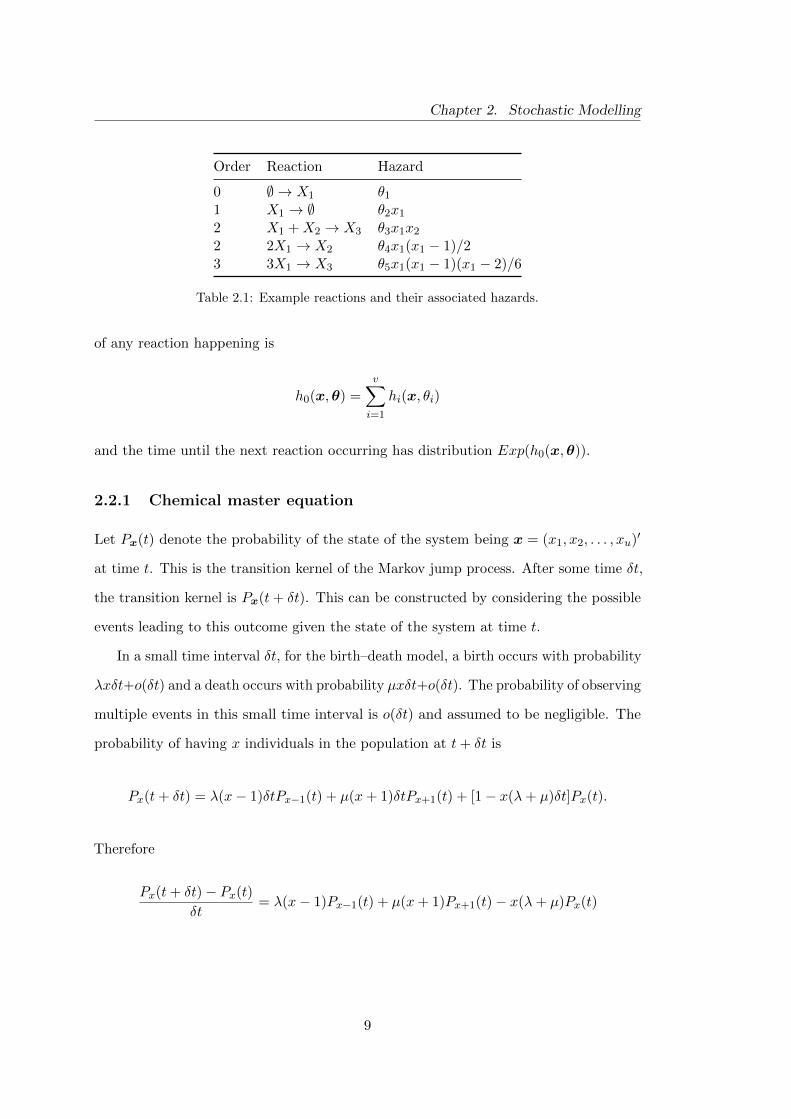
Order Reaction Hazard
0 ∅ → X1 θ11 X1 → ∅ θ2x12 X1 +X2 → X3 θ3x1x22 2X1 → X2 θ4x1(x1 − 1)/23 3X1 → X3 θ5x1(x1 − 1)(x1 − 2)/6
Table 2.1: Example reactions and their associated hazards.
of any reaction happening is
h0(x,θ) =v∑i=1
hi(x, θi)
and the time until the next reaction occurring has distribution Exp(h0(x,θ)).
2.2.1 Chemical master equation
Let Px(t) denote the probability of the state of the system being x = (x1, x2, . . . , xu)′
at time t. This is the transition kernel of the Markov jump process. After some time δt,
the transition kernel is Px(t+ δt). This can be constructed by considering the possible
events leading to this outcome given the state of the system at time t.
In a small time interval δt, for the birth–death model, a birth occurs with probability
λxδt+o(δt) and a death occurs with probability µxδt+o(δt). The probability of observing
multiple events in this small time interval is o(δt) and assumed to be negligible. The
probability of having x individuals in the population at t+ δt is
Px(t+ δt) = λ(x− 1)δtPx−1(t) + µ(x+ 1)δtPx+1(t) + [1− x(λ+ µ)δt]Px(t).
Therefore
Px(t+ δt)− Px(t)
δt= λ(x− 1)Px−1(t) + µ(x+ 1)Px+1(t)− x(λ+ µ)Px(t)
9

Chapter 2. Stochastic Modelling
and taking the limit as δt→ 0 gives the Chemical Master Equation (CME)
dPx(t)
dt= λ(x− 1)P (t)x−1 − x(λ+ µ)P (t)x + µ(x+ 1)P (t)x+1.
For a general model, the CME is given by
dPx(t)
dt=
v∑i=1
{hi(x− Si, ci)Px−Si(t)− hi(x, ci)Px(t)
}
where Si represents the ith column of the stoichiometry matrix.
2.2.2 The direct method
This algorithm, in the context of stochastic kinetic models was introduced by Gillespie
(1977) and is often referred to as the Gillespie algorithm. It can be used to simulate exact
trajectories from a stochastic model. The detailed algorithm is given in Algorithm 1.
At each iteration of the Gillespie algorithm, the time until the next reaction is
simulated as an exponential random variable (Step 4). The rate is given by the sum of
hazards of each reaction happening which have been calculated in Steps 2 and 3. Once
the time until the next reaction has been simulated, the type of reaction must also be
simulated. This is done by simulating from a discrete distribution with probabilities
given by
hi(x, θi)
h0(x,θ)for i = 1, . . . , v.
Three realisations from the birth–death model are given in Figure 2.1 for a particular
choice of parameters and initial population level x0. For these simulations, µ > λ hence
the population will eventually die out. It can be seen that in these three simulations,
the populations become extinct at times t ≈ (3.4, 5.2, 6.0).
10

Chapter 2. Stochastic Modelling
Algorithm 1 Stochastic simulation: Gillespie’s direct method
1. Set t = 0. Initialise the rate constants θ = (θ1, . . . , θv)′ and the initial molecule
numbers x = (x1, . . . , xu)′.
2. Calculate the hazard hi(x, θi) for each potential reaction i = 1, . . . , v.
3. Calculate the combined hazard h0(x,θ) =∑v
i=1 hi(x, θi).
4. Simulate the time until the next reaction, t∗ ∼ Exp(h0(x,θ)) and set t := t+ t∗.
5. Simulate the reaction index, j, as a discrete random quantity with probabilitieshi(x, θi)/h0(x,θ), i = 1, . . . , v.
6. Update the state x according to reaction j.
7. Output x and t. If t < Tmax, return to step 2.
Label Reaction Hazard Description
R1 X → 2X h1(x, λ) = λx Birth
R2 X → ∅ h2(x, µ) = µx Death
Table 2.2: Reactions and their hazards for the birth–death model.
2.3 Example: the birth–death model
The simple birth–death process is a well documented stochastic model. It was first
introduced by Yule (1925) and Feller W. (1939) in the context of population growth.
It has been widely used in biological applications, for example Kendall (1948) uses it to
model the early stages of an epidemic. Novozhilov (2006) discusses the suitability of the
birth–death model for modelling biological processes; the state space is discrete rather
than continuous, ideal for describing counts such as cells or genes.
For the birth–death model, X represents a population and x represents the number
of individuals present, rather than a number of molecules of a chemical species. In
this model only two events can happen: either a birth or a death. In chemical kinetic
notation this system is represented in Table 2.2, where R1 denotes a birth event which
happens with rate λ and R2 denotes a death event which happens with rate µ.
11

Chapter 2. Stochastic Modelling
0
5
10
15
0 2 4 6Time
Pop
ulat
ion
leve
l (X
)
Figure 2.1: Three realisations from the birth–death model for x0 = 10, λ = 0.6 and µ = 1.
2.4 Example: mitochondrial DNA model
Neurons are specialised types of cell in the human body and are a fundamental aspect of
the nervous system. The idea that the loss of neurons in the substantia nigra region of
the human brain is implicated in Parkinson’s disease dates back to the work of Hassler
(1938) and Fearnley and Lees (1991). Bender et al. (2006) observed that patients with
Parkinson’s disease exhibited higher than average levels of mitochondrial DNA (mtDNA)
deletions in the substantia nigra region of the brain. However, the mechanism which
these mtDNA deletions play in disease is still poorly understood.
A model was developed by Henderson et al. (2009) to explore the relationship
between mtDNA and cell death. The model is based on the ideas of Elson et al.
(2001) who suggest that the relaxed replication of mtDNA is responsible for the the
accumulation of mutant mtDNA through random genetic drift.
The model involves two chemical species X = (X1, X2)′ where X1 represents healthy
mtDNA and X2 represents unhealthy mtDNA (mtDNA with deletions). The total
number of mtDNA present in the cell is given by x1 + x2.
12
Chapter 2. Stochastic Modelling
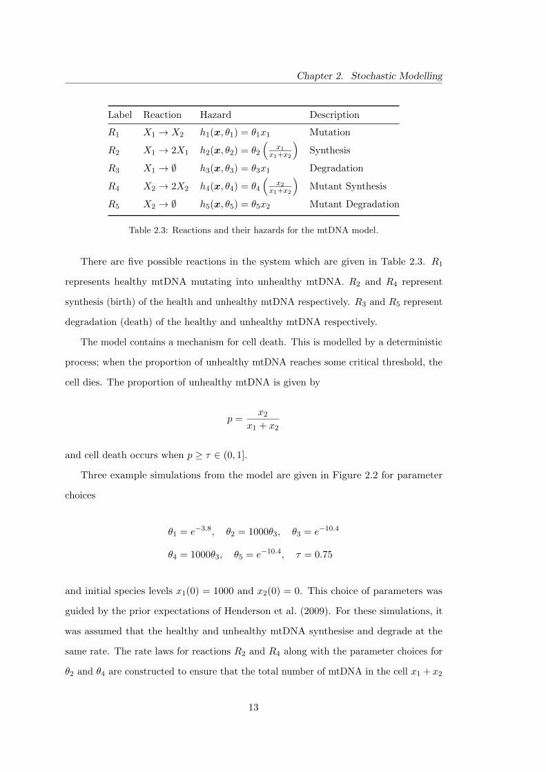
Label Reaction Hazard Description
R1 X1 → X2 h1(x, θ1) = θ1x1 Mutation
R2 X1 → 2X1 h2(x, θ2) = θ2
(x1
x1+x2
)Synthesis
R3 X1 → ∅ h3(x, θ3) = θ3x1 Degradation
R4 X2 → 2X2 h4(x, θ4) = θ4
(x2
x1+x2
)Mutant Synthesis
R5 X2 → ∅ h5(x, θ5) = θ5x2 Mutant Degradation
Table 2.3: Reactions and their hazards for the mtDNA model.
There are five possible reactions in the system which are given in Table 2.3. R1
represents healthy mtDNA mutating into unhealthy mtDNA. R2 and R4 represent
synthesis (birth) of the health and unhealthy mtDNA respectively. R3 and R5 represent
degradation (death) of the healthy and unhealthy mtDNA respectively.
The model contains a mechanism for cell death. This is modelled by a deterministic
process; when the proportion of unhealthy mtDNA reaches some critical threshold, the
cell dies. The proportion of unhealthy mtDNA is given by
p =x2
x1 + x2
and cell death occurs when p ≥ τ ∈ (0, 1].
Three example simulations from the model are given in Figure 2.2 for parameter
choices
θ1 = e−3.8, θ2 = 1000θ3, θ3 = e−10.4
θ4 = 1000θ3, θ5 = e−10.4, τ = 0.75
and initial species levels x1(0) = 1000 and x2(0) = 0. This choice of parameters was
guided by the prior expectations of Henderson et al. (2009). For these simulations, it
was assumed that the healthy and unhealthy mtDNA synthesise and degrade at the
same rate. The rate laws for reactions R2 and R4 along with the parameter choices for
θ2 and θ4 are constructed to ensure that the total number of mtDNA in the cell x1 + x2
13

Chapter 2. Stochastic Modelling
X1 X2
0
300
600
900
0 10000 20000 30000 0 10000 20000 30000
Time
Pop
ulat
ion
Figure 2.2: Three realisations from the mtDNA model.
remains approximately constant (at 1000) throughout the lifetime of the cell.
It can be seen that for this choice of parameters, the number of healthy mtDNA
decrease over time and correspondingly the number of unhealthy mtDNA increase.
When the proportion of unhealthy mtDNA reaches the lethal threshold (τ = 0.75 in
these simulations), the cell dies.
2.5 Example: the PolyQ model
The PolyQ model was briefly introduced in Chapter 1. It is a large model containing 25
chemical species and 69 reactions. The chemical species are listed in Table 2.4 and the
reactions in Table 2.5.
Cell death can occur via two biological pathways, either via proteasome inhibition or
p38MAPK activation. The dummy species PIdeath and p38death are included in the
model to encode cell death via these pathways. These species are both binary variables
which take the value zero while the cell is alive. When death occurs, either PIdeath = 1
or p38death = 1 depending on the death pathway.
An event in the PolyQ model is triggered when either PIdeath > 0 and p38death > 0,
this changes the value of kalive from 0 to 1. kalive is a dummy rate parameter which is
14

Chapter 2. Stochastic Modelling
present in every reaction (omitted from the rates in Table 2.5), when it is zero, this has
the effect of preventing more reactions happening and inducing cell death in the model.
15

Chapter 2. Stochastic Modelling
Name Description Initial amount
PolyQ Polyglutamine-containing protein 1000mRFPu Red fluorescent protein 300Proteasome 26S Proteasome 1000PolyQProteasome PolyQ bound to proteasome 0mRFPuProteasome mRFPu bound to proteasome 0AggPolyQi PolyQ aggregate of size i (i = 1, . . . , 5) 0SeqAggP Inclusion 0AggPProteasome Aggregated protein bound to proteasome 0ROS Reactive oxygen species 10p38P Active P38MAPK 0p38 Inactive p38MAPK 100NatP Generic pool of native protein 19500MisP Misfolded protein 0MisPProteasome Misfolded protein bound to proteasome 0AggPi Small aggregate of size i (i = 1, . . . , 5) 0PIdeath Dummy species to record cell death due to proteasome inhibition 0p38death Dummy species to record cell death due to p38MAPK activation 0
Table 2.4: Species involved in the PolyQ model and their initial amounts.
ID Reaction name Reaction Rate law
1 PolyQ synthesis Source → PolyQ ksynPolyQ
2 PolyQ/proteasome binding PolyQ + Proteasome → PolyQProteasome kbinPolyQ[PolyQ][Proteasome]
3 PolyQ/proteasome release PolyQProteasome → PolyQ + Proteasome krelPolyQ[PolyQProteasome]
4 PolyQ degradation PolyQProteasome → Proteasome kkdegPolyQkproteff [PolyQProteasome]
5 mRFPu synthesis Source → mRFPu ksynmRFPu
6 mRFPu/proteasome binding mRFPu + Proteasome → mRFPuProteasome kbinmRFPu[mRFPu][Proteasome]
7 mRFPu/proteasome release mRFPuProteasome → mRFPu + Proteasome krelmRFPu[mRFPuProteasome]
8 mRFPu degradation mRFPuProteasome → Proteasome kdegmRFPukproteff[mRFPuProteasome]
9 Aggregation 2PolyQ + ROS → AggPolyQ1 + ROS kaggPolyQ [PolyQ][PolyQ-1][ROS2]
0.5(102 + [ROS2])
10 Aggregation growth AggPolyQ1 AggPolyQ1 + PolyQ + ROS kaggPolyQ[AggPolyQ1][PolyQ][ROS2]
→ AggPolyQ2+ ROS /(102 + [ROS2])
11 Aggregation growth AggPolyQ2 AggPolyQ2 + PolyQ + ROS kaggPolyQ[AggPolyQ2][PolyQ][ROS2]
→ AggPolyQ3+ ROS /(102 + [ROS2])
12 Aggregation growth AggPolyQ3 AggPolyQ3 + PolyQ + ROS kaggPolyQ[AggPolyQ3][PolyQ][ROS2]
→ AggPolyQ4+ ROS /(102 + [ROS2])
13 Aggregation growth AggPolyQ4 AggPolyQ4 + PolyQ + ROS kaggPolyQ[AggPolyQ4][PolyQ][ROS2]
→ AggPolyQ5+ ROS /(102 + [ROS2])
14a PolyQ disaggregation 1 AggPolyQ1 → 2AggPolyQ kdissaggPolyQ1[AggPolyQ1]
14b PolyQ disaggregation 2 AggPolyQ2 → AggPolyQ1 + PolyQ kdissaggPolyQ2[AggPolyQ2]
14c PolyQ disaggregation 3 AggPolyQ3 → AggPolyQ2 + PolyQ kdissaggPolyQ3[AggPolyQ3]
14d PolyQ disaggregation 4 AggPolyQ4 → AggPolyQ3 + PolyQ kdissaggPolyQ4[AggPolyQ4]
16

Chapter 2. Stochastic Modelling
14e PolyQ disaggregation 5 AggPolyQ5 → AggPolyQ4 + PolyQ kdissaggPolyQ5[AggPolyQ5]
15 Inclusion formation AggPolyQ5 + PolyQ → 7SeqAggP kaggPolyQ[AggPolyQ5][PolyQ]
16 Inclusion growth SegAggP + PolyQ → 2SeqAggP kseqPolyQ[SeqAggP][PolyQ]
17a Proteasome inhibition AggPolyQ1 + Proteasome → kinhprot[AggPPolyQ1][Proteasome]
by aggregates 1 AggPProteasome
17b Proteasome inhibition AggPolyQ2 + Proteasome → kinhprot[AggPPolyQ2][Proteasome]
by aggregates 2 AggPProteasome
17c Proteasome inhibition AggPolyQ3 + Proteasome → kinhprot[AggPPolyQ3][Proteasome]
by aggregates 3 AggPProteasome
17d Proteasome inhibition AggPolyQ4 + Proteasome → kinhprot[AggPPolyQ4][Proteasome]
by aggregates 4 AggPProteasome
17e Proteasome inhibition AggPolyQ5 + Proteasome → kinhprot[AggPPolyQ5][Proteasome]
by aggregates 5 AggPProteasome
18 Basal ROS production Source → ROS kgenROS
19 ROS removal ROS → Sink kremROS[ROS]
20a ROS generation AggPolyQ1 AggPolyQ1 → AggPolyQ1 + ROS kgenROSAggP [AggPolyQ1]
20b ROS generation AggPolyQ2 AggPolyQ2 → AggPolyQ2 + ROS kgenROSAggP [AggPolyQ2]
20c ROS generation AggPolyQ3 AggPolyQ3 → AggPolyQ3 + ROS kgenROSAggP [AggPolyQ3]
20d ROS generation AggPolyQ4 AggPolyQ4 → AggPolyQ4 + ROS kgenROSAggP [AggPolyQ4]
20e ROS generation AggPolyQ5 AggPolyQ5 → AggPolyQ5 + ROS kgenROSAggP [AggPolyQ5]
21 ROS generation AggP Proteasome AggPProteasome kgenROSAggP [AppPProteasome]
→ AggPProteasome + ROS
22 p38MAPK activation ROS + p38 → ROS + p38P kactp38[ROS][p38]
23 p38MAPK inactivation p38P → p38 kinactp38[p38P]
24 AggPProteasome sequestering AggPProteasome + SeqAggP → 2SeqAggP kseqAggPProt[AggPProteasome][SeqAggP]
25 PolyQProteasome sequestering PolyQProteasome + SeqAggP → 2SeqAggP kseqPolyQProt[PolyQProteasome][SeqAggP]
26 Protein synthesis Source → NatP ksynNatP
27 Protein misfolding NatP + ROS → MisP + ROS kmisfold[NatP][ROS]
28 Protein refolding MisP → NatP krefold[MisP]
29 MisP/Proteasome binding MisP + Proteasome → MisPProteasome kbinMisPProt[MisP][Proteasome]
30 MisPProteasome release MisPProteasome → MisP + Proteasome krelMisPProt[MisPProteasome]
31 Degradation of misfolded protein MisPProteasome → Proteasome kdegMisP kproteff[MisPProteasome]
32 Aggregation of misfolded protein 2MisP → AggP1 kaggMisP [MisP][MisP -1]/2
33a Aggregation growth 1 AggP1 + MisP → AggP2 kagg2MisP [MisP][AggP1]
33b Aggregation growth 2 AggP2 + MisP → AggP3 kagg2MisP [MisP][AggP2]
33c Aggregation growth 3 AggP3 + MisP → AggP4 kagg2MisP [MisP][AggP3]
33d Aggregation growth 4 AggP4 + MisP → AggP5 kagg2MisP [MisP][AggP4]
34a Disaggregation 1 AggP1 → 2MisP kdiasaggMisP1[AggP1]
34b Disaggregation 2 AggP2 → AggP1 + MisP kdiasaggMisP2[AggP2]
34c Disaggregation 3 AggP3 → AggP2 + MisP kdiasaggMisP3[AggP3]
34d Disaggregation 4 AggP4 → AggP3 + MisP kdiasaggMisP4[AggP4]
17

Chapter 2. Stochastic Modelling
34e Disaggregation 5 AggP5 → AggP4 + MisP kdiasaggMisP5[AggP5]
35 MisP Inclusion formation AggP5 + MisP → 7SeqAggP kagg2MisP [AggP5][MisP]
36 MisP Inclusion growth SeqAggP + MisP → 2SeqAggP kseqMisP [SeqAggP][MisP]
37a Proteasome inhibition AggP1 AggP1 + Proteasome → kinhprot[AggP1][Proteasome]
AggPProteasome
37b Proteasome inhibition AggP2 AggP2 + Proteasome → kinhprot[AggP2][Proteasome]
AggPProteasome
37c Proteasome inhibition AggP3 AggP3 + Proteasome → kinhprot[AggP3][Proteasome]
AggPProteasome
37d Proteasome inhibition AggP4 AggP4 + Proteasome→ kinhprot[AggP4][Proteasome]
AggPProteasome
37e Proteasome inhibition AggP5 AggP5 + Proteasome → kinhprot[AggP5][Proteasome]
AggPProteasome
38a ROS generation AggP1 AggP1 → AggP1 + ROS kgenROSAggP [AggP1]
38b ROS generation AggP2 AggP2 → AggP2 + ROS kgenROSAggP [AggP2]
38c ROS generation AggP3 AggP3 → AggP3 + ROS kgenROSAggP [AggP3]
38d ROS generation AggP4 AggP4 → AggP4 + ROS kgenROSAggP [AggP4]
38e ROS generation AggP5 AggP5 → AggP5 + ROS kgenROSAggP [AggP5]
39 p38 ROS generation p38P → p38P + ROS kgenROSp38kkp38act[p38P]
40 SeqAggP ROS generation SeqAggP → SeqAggP + ROS kgenROSseqAggP [SeqAggP]
41 p38 cell death p38P → p38P + p38death kp38deathkp38act[p38P]
42 PI cell death AggPProteasome → kPIdeath[AggPProteasome]
AggPProteasome + PIdeath
Table 2.5: List of reactions and hazards for the PolyQ model
Three example realisations from the model are given in Figure 2.3. It can be seen that
the cells represented in blue and green both die via the p38death pathway and the cell
represented in red dies via the PIdeath pathway.
18

Chapter 2. Stochastic Modelling
PolyQ Proteasome NatP MisP
MisP_Proteasome AggP1 AggP2 AggP3
AggP4 AggP5 AggPolyQ1 AggPolyQ2
AggPolyQ3 AggPolyQ4 AggPolyQ5 SeqAggP
AggP_Proteasome mRFPu mRFPu_Proteasome PolyQ_Proteasome
ROS p38_P p38 Source
Sink p38death PIdeath
0
250
500
750
1000
0
250
500
750
1000
0
20000
40000
60000
0e+00
5e+04
1e+05
0
100
200
0
1000
2000
3000
0
500
1000
1500
0
200
400
0
50
100
150
0
10
20
30
40
0
30
60
90
0
20
40
60
0
5
10
15
20
0.0
2.5
5.0
7.5
10.0
0
1
2
3
4
0e+00
1e+05
2e+05
3e+05
0
100
200
300
0
2000
4000
6000
0
10
20
30
40
0
5
10
15
20
0
200
400
600
0
20
40
60
40
60
80
100
0.50
0.75
1.00
1.25
1.50
0
3000
6000
9000
0.00
0.25
0.50
0.75
1.00
0.00
0.25
0.50
0.75
1.00
0e+00 1e+05 2e+05 0e+00 1e+05 2e+05 0e+00 1e+05 2e+05
Time
Leve
l of c
hem
ical
spe
cies
Figure 2.3: Three realisations from the PolyQ model
19

Chapter 2. Stochastic Modelling
2.6 Other simulation strategies
For most models of interest, the Markov jump process is typically not analytically
tractable. However, the simplicity of the birth–death means that it is possible to
find an analytic expression for the transition probability; further details are given in
Chapter 4. For the mtDNA and PolyQ models, no analytic results exist for the transition
probabilities.
It is simple to simulate realisations from such models. The ability to simulate from
a model allows it properties to be studied. Simulation strategies can broadly be divided
into exact, approximate and hybrid methods.
2.6.1 Exact simulation strategies
Using an exact simulation strategy produces an exact realisation from the Markov jump
process. The disadvantage of using exact simulations strategies is that they have the
potential to be computationally expensive.
The Gibson-Bruck algorithm
The Gibson-Bruck algorithm (Gibson and Bruck, 2000) is another example of an exact
simulation strategy. This is based on an alternative version of Gillespie’s algorithm
named the First Reaction Method (Gillespie, 1976) and is generally considered to be
the fastest and most efficient exact method.
Gibson and Bruck (2000) use the notion of a dependency graph that has a vertex for
each reaction. A directed edge is present between two vertices a and b if the occurrence
of reaction a causes the state of the system to be altered in such a way that the hazard
of reaction b is changed. This graph can then be used to update only the hazards which
need to be updated after each reaction event, rather than all hazards.
20

Chapter 2. Stochastic Modelling
2.6.2 Approximate simulation strategies
While exact methods for simulation such as the Gillespie algorithm are preferable,
they have the potential to be very slow, especially when the model is complex. Large
speed-ups can be gained by using an approximate method which still captures the vital
kinetics of the model but does not necessarily simulate every reaction.
τ-leap method
The τ -leap method of Gillespie (2001) approximates the numbers of each type of reaction
occurring in a small interval, by assuming they are independent Poisson random variables.
Simulation proceeds by choosing a variable time interval τ and simulating the number
of reactions of type i from a Po(hi(x, θi)τ), for each reaction i = 1, . . . , v. The time is
then updated to t := t+ τ and the states updated accordingly.
The accuracy of the algorithm depends on the size of τ chosen, smaller τ leads to a
more accurate algorithm. For large τ , the assumption that the hazards are constant
over the interval becomes less realistic. As a consequence, assuming that the number of
occurrences of each type of reaction are independent Poisson random variables is less
reliable. However, the algorithm will run faster for larger τ , thus τ represents a trade
off between accuracy and speed.
For any interval τ , where at least one reaction has occurred, the assumption that
the hazard is constant over the interval may not hold. This is because, the occurrence
of any reaction changes the state of the system. Reactions with hazards above zero
order depend on the state of the system. Consequently, a change in the state causes the
hazard to change.
The size of τ chosen at each step is designed to ensure that the disruption to the
assumption of constant hazard is within some acceptable tolerance which is a proportion
of the cumulative hazard. The expected new states x∗ after time τ can easily be
calculated and the hazards at these expected new states evaluated. Gillespie (2001)
suggests that the chosen τ should ensure that, for each reaction, the difference in hazard
21
Chapter 2. Stochastic Modelling
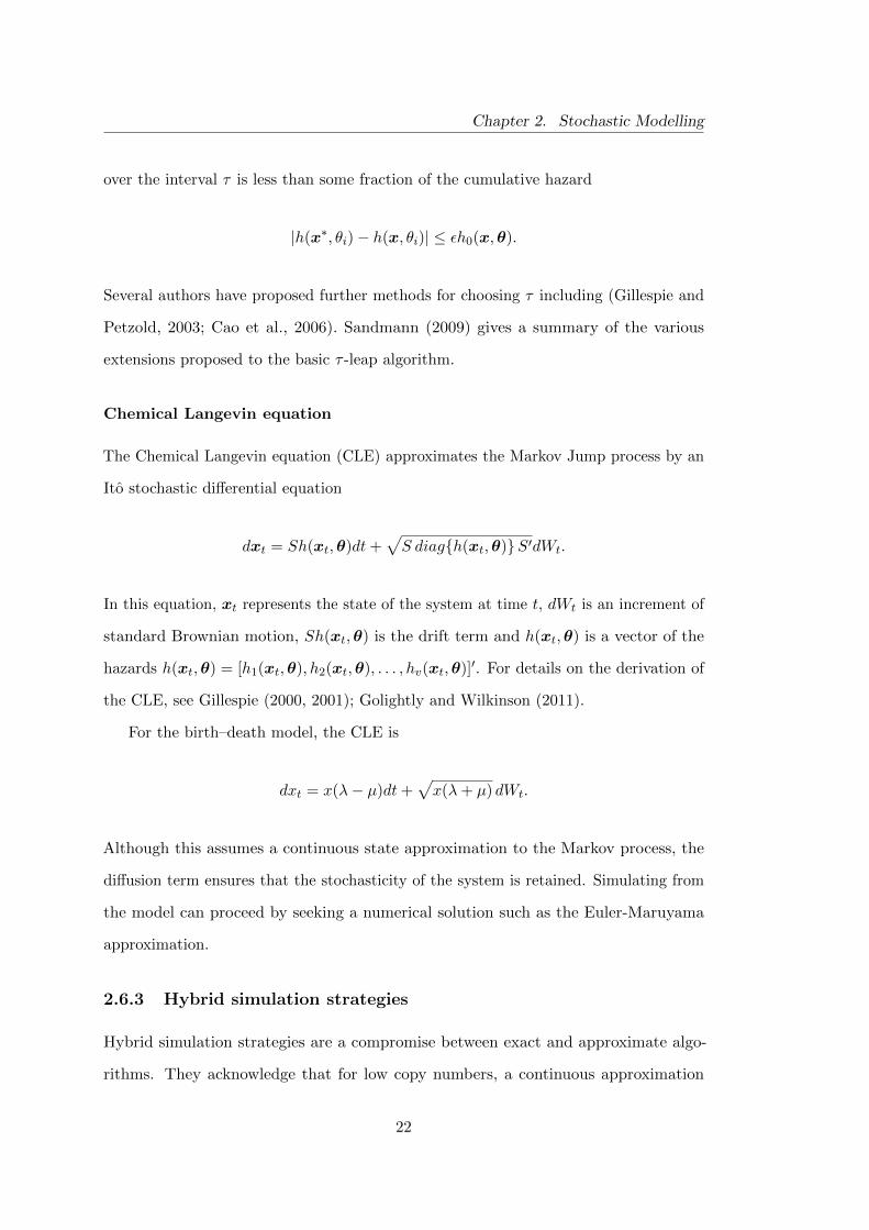
over the interval τ is less than some fraction of the cumulative hazard
|h(x∗, θi)− h(x, θi)| ≤ εh0(x,θ).
Several authors have proposed further methods for choosing τ including (Gillespie and
Petzold, 2003; Cao et al., 2006). Sandmann (2009) gives a summary of the various
extensions proposed to the basic τ -leap algorithm.
Chemical Langevin equation
The Chemical Langevin equation (CLE) approximates the Markov Jump process by an
Ito stochastic differential equation
dxt = Sh(xt,θ)dt+√S diag{h(xt,θ)}S′dWt.
In this equation, xt represents the state of the system at time t, dWt is an increment of
standard Brownian motion, Sh(xt,θ) is the drift term and h(xt,θ) is a vector of the
hazards h(xt,θ) = [h1(xt,θ), h2(xt,θ), . . . , hv(xt,θ)]′. For details on the derivation of
the CLE, see Gillespie (2000, 2001); Golightly and Wilkinson (2011).
For the birth–death model, the CLE is
dxt = x(λ− µ)dt+√x(λ+ µ) dWt.
Although this assumes a continuous state approximation to the Markov process, the
diffusion term ensures that the stochasticity of the system is retained. Simulating from
the model can proceed by seeking a numerical solution such as the Euler-Maruyama
approximation.
2.6.3 Hybrid simulation strategies
Hybrid simulation strategies are a compromise between exact and approximate algo-
rithms. They acknowledge that for low copy numbers, a continuous approximation
22

Chapter 2. Stochastic Modelling
which ignores the inherent discreteness is inappropriate. However they exploit the fact
that for large copy numbers, a fast approximation is satisfactory.
The computational cost of running an exact simulation strategy is directly propor-
tional to the number of reactions which happen in the system. If certain reactions
happen very frequently then this can cause the algorithm to slow down significantly.
In general, hybrid algorithms class reactions as either fast or slow. This is typically
done by partitioning the chemical species into those that must be modelled discretely
and those which can be modelled by a continuous approximation. Any reaction involving
at least one chemical species which is modelled discretely is labelled as a slow reaction
and and all other reactions as fast.
The following gives an overview of a generic hybrid simulation scheme. At each
iteration of the scheme, reactions are classified as fast or slow based on the current
state of the system xt. For a chosen time-step δt, a path is sampled over (t, t+ δt) for
the fast reactions using the fast approximation. The slow reaction hazards are then
evaluated to decide whether or not a slow reaction happened in (t, t+ δt). If no slow
reaction occurred in this time interval, then time is updated to t := t + δt and the
state of the system is updated according to the proposed values from the fast reactions.
If one or more slow reaction does occur then let t′ denote the time at which the first
slow reaction happened. Update time to t := t+ t′ and update the state of the system
according to the first slow reaction.
In this setup, only time intervals in which slow reactions happen require exact
simulation. Intervals where no slow reactions happen are simulated using the fast
approximation, thus a saving in computational time is achieved.
One specific approach to hybrid simulation is to represent the fast reactions via an
ODE which can be approximated numerically (Alfonsi et al., 2005; Kiehl et al., 2004).
Other authors use the CLE to approximate the fast reactions (Salis and Kaznessis,
2005; Higham et al., 2011). Puchaka and Kierzek (2004) use a combination of the
Gibson-Bruck algorithm for the slow reactions and the τ -leap algorithm for the fast
reactions.
23

Chapter 3
Bayesian inference
The aim of this thesis is to perform statistical inference for the parameters of a large
stochastic kinetic model, based on experimental data. Inference will be approached in
the Bayesian framework. A particular problem with such methods is that the likelihood
is intractable. The PolyQ model, which was introduced in Chapter 1, is an example
of such a model. This chapter begins by introducing the notion of state–space models
before giving an overview of the concepts behind Bayesian inference. Several schemes
for implementing parameter inference are outlined.
3.1 State–space models
Consider a dynamical system consisting of states which change over time. State–space
models describe the time evolution of such a system. Let x1,x2, . . . ,xT represent states
of the system where xt is the value of the process at time t. In general, the states will
depend on parameters θ. The states evolve according to the state equation
π(xt+1|x1,x2, . . . ,xt,θ) = π(xt+1|xt,θ)
and since xt+1 is dependent only on xt and no other previous states, the evolution is
Markovian.
Let y1,y2, . . . ,yT be observations of unobserved latent states x1,x2, . . . ,xT . Con-
24

Chapter 3. Bayesian inference
&%'$xt−1 &%
'$xt &%
'$xt+1
yt−1 yt yt+1
-- -- -
? ? ?
Figure 3.1: DAG representation of a state–space model.
sider the birth-death example – suppose that observing the exact population level is
impossible. In this situation, the xt remain unobserved, however the population level
can be observed with some error; the noisy observations are the yt. For example, the
error model could be Gaussian
yt|xt ∼ N(xt, σ2I),
where I is the identity matrix of appropriate dimension. The observations yt are
conditionally independent given the states xt and the parameters θ. The conditional
distribution of yt is
π(yt|x1,x2, . . . ,xt,y1,y2, . . . ,yt−1,θ) = π(yt|xt,θ).
That is, given the latent states, the observations are conditionally independent. This
set up is pictured schematically in Figure 3.1.
3.2 Introduction to Bayesian inference
The goal is to quantify uncertainty about parameters θ = (θ1, θ2, . . . , θp)′ using observed
data y. Suppose y is modelled by some probability density function fy(y|θ), then the
25

Chapter 3. Bayesian inference
likelihood is defined as
L(θ|y) = fy(y|θ).
The likelihood represents the probability distribution of the data y as a function of
the parameters θ. Prior beliefs about θ are represented by the density π(θ) and Bayes’
Theorem provides a way of updating these beliefs based upon observed data. The
posterior distribution
π(θ|y) =π(θ)L(θ|y)∫
θ π(θ)L(θ|y) dθ, (3.1)
represents the updated beliefs about θ after observing the data y. Since the denominator
of Equation 3.1 is not a function of θ, it can be regarded as a constant of proportionality
and thus
π(θ|y) ∝ π(θ)× L(θ|y),
Posterior ∝ Prior× Likelihood.
3.3 Markov chain Monte Carlo (MCMC)
In general, obtaining the constant of proportionality (the denominator of Equation 3.1)
is a non–trivial problem for anything but the very simplest of cases. It involves the
integral ∫θπ(θ)L(θ|y) dθ
which is often non–standard and multidimensional. Also of interest is calculating
moments of the posterior distribution such as means, variances and marginal and
conditional distributions. Markov chain Monte Carlo (MCMC) algorithms draw samples
from the desired density, without knowledge of the normalising constant.
Metropolis–Hastings
The Metropolis–Hastings algorithm can be used to sample from the density of interest
π(θ|y). The algorithm was developed by Metropolis et al. (1953) and later generalised
26
Chapter 3. Bayesian inference
Algorithm 2 Metropolis–Hastings algorithm
Initialise the state of the chain θ(0).
For each iteration of the scheme:
1. Sample θ∗ ∼ q(·|θ) where q is some proposal distribution.
2. Compute the acceptance probability
α(θ∗|θ) = min
{1,π(θ∗)
π(θ)
π(y|θ∗)π(y|θ)
q(θ|θ∗)q(θ∗|θ)
.
}3. Set θ = θ∗ with probability α(θ∗|θ), otherwise retain θ.
by Hastings (1970). The idea is to construct a Markov chain with stationary distribution
equal to the target distribution; the details are given in Algorithm 2.
Step 1 of the algorithm generates a proposed parameter value denoted θ∗ from an
easy to simulate from transition kernel, q(θ∗|θ(i−1)), known as the proposal distribution,
which should have the same support as the target. At each iteration, a new value θ∗
is generated from the proposal distribution, this new value depends on the previous
state of the chain θ(i−1). The proposed value is either accepted or rejected resulting
in the chain either moving to θ∗ or staying at its current value. The accept/reject
move depends on the acceptance probability α(θ∗|θ(i−1)), which in turn depends on
the proposal distribution and π(·|y). Crucially, the dependence on π(·|y) is only in the
form of a ratio, and therefore the target distribution only needs to be known up to a
constant of proportionality.
Choice of proposal distribution
A special case of the Metropolis-Hastings algorithm arises when a symmetric proposal
distribution is used
q(θ∗|θ) = q(θ|θ∗).
27

Chapter 3. Bayesian inference
Here the ratio of proposal densities cancels and the acceptance probability simplifies to
α(θ∗|θ) = min
{1,π(θ∗)
π(θ)
π(y|θ∗)π(y|θ)
}.
In this case, whenever a θ∗ is proposed which moves the chain to an area of higher
posterior density than previously, it will be accepted with certainty.
Another special case of the Metropolis–Hastings algorithm is the scenario in which
the proposal distribution is chosen so that it does not depend on the current value of
the chain, i.e. q(θ∗|θ) = f(θ∗) for some density f . Here the acceptance probability
simplifies to
α(θ∗|θ) = min
{1,π(θ∗)
π(θ)
π(y|θ∗)π(y|θ)
f(θ)
f(θ∗)
}
= min
1,π(θ∗)π(y|θ∗)
/π(θ)π(y|θ)
f(θ∗)/f(θ)
.
It can be seen that the acceptance ratio can be controlled by the similarity of f(·) and
π(·|y). Choosing an f(·) that is very close to π(·)π(y|·) will ensure a high acceptance
probability.
If the proposal distribution q takes the form
θ∗ = θ + ω
where ω are independent identically distributed random variates (known as innovations),
then this special case of the Metropolis algorithm is known as a random walk sampler.
Common choices of distribution for ω are uniform and Gaussian, with mean zero.
Choice of tuning parameters
The mixing of the MCMC scheme refers to how well the chain moves around the space
and consequently how long it takes for the chain to converge. The parameters that
govern the distribution of ω will determine how well the chain mixes. Suppose ω follows
28
Chapter 3. Bayesian inference
a multivariate normal distribution such that
ω ∼ N(0, V ),
then V must be carefully chosen to ensure good mixing. If the variance is too low then
small moves will be proposed and the chain will explore the space too slowly. If the
variance is too big then large moves will be proposed, most of which will be rejected
meaning that chain will move too little. Taking into account the correlation in θ by
allowing V to have non–zero off–diagonal elements is important to ensure the space is
explored efficiently.
It has been suggested that when the target distribution is Gaussian, an acceptance
probability of 0.234 is optimal (Roberts and Rosenthal, 2001). However, this result
has been extended to elliptically symmetric targets (Sherlock and Roberts, 2009) and
more recently Sherlock (2013) give a general set of sufficient conditions under which an
acceptance probability of 0.234 is optimal. Gelman et al. (1996); Roberts et al. (1997);
Roberts and Rosenthal (2001) suggest that the random walk should be tuned such that
V =2.382Σπ
p
where Σπ is the covariance matrix of the target distribution π and p is the dimension
of θ. Although Σπ is not typically available, an estimate can be obtained from one or
more pilot runs of the scheme.
Analysis of MCMC output
To ensure a scheme such as Metropolis Hastings samples from the target probability
distribution, convergence must be carefully monitored. Samples obtained before the
chain has converged are known as burn–in and should be discarded. Convergence can
be checked informally using graphical methods. These include viewing trace plots of
the output to check for irregularities and using an autocorrelation plot to monitor the
29

Chapter 3. Bayesian inference
autocorrelation in the chain at different lags.
More formal ideas for detecting convergence have been proposed by several authors
including Gelman and Rubin (1992), who suggest initialising multiple chains in different
places and checking they become indistinguishable after some time. There are a series
of more formal checks for assessing convergence by other authors, see Heidelberger and
Welch (1983) and Geweke (1992). If the autocorrelation is high then the chains can be
thinned which involves keeping only every ith iteration, ensuring subsequent samples
are independent. Raferty and Lewis (1992) give guidelines on how to pick the length of
the burn–in to discard and by how much the chain should be thinned based on the user
specifying how accurate they would like the posterior summaries to be.
Once the chain has reached convergence and it is sampling from the distribution
of interest, the output can be analysed. It is trivial to compute estimates of summary
statistics such as marginal means and variances. Plotting histograms or density plots
gives an idea of the shape of marginal distributions.
3.4 Likelihood free inference
The motivation for likelihood free inference are models which have intractable likelihoods,
for example the complex PolyQ model described in Chapter 1. In such cases, it is
typically not possible to evaluate the likelihood although it is possible to simulate from
the model. Recent interest has turned to methods for inference which do not require
the likelihood to be evaluated and the ideas behind these methods date back to Diggle
and Gratton (1984).
The general idea behind likelihood free inference involves utilising the ability to
simulate from the model for the latent states, that is, obtain realisations from π(x|θ)
for different choices of θ, without needing to evaluate this density. For example, using
the Gillespie algorithm described in Section 2.2.2 of Chapter 2 it is simple to obtain
realisations from the model for a given set of parameters and initial conditions. The
simulated datasets are then compared to the observed data.
30
Chapter 3. Bayesian inference
Approximate Bayesian computation (ABC) is an example of a likelihood-free method
for inference and it was first applied (in its current form) to problems in population
genetics by Tavare et al. (1997) and Pritchard et al. (1999). The idea is to generate
many synthetic datasets from the model for different parameter choices and compare the
simulated data to the observed data. Typically, ABC schemes will compare summary
statistics of the simulated datasets with summary statistics from the observed data.
Crucially ABC methods do not generate samples from the true posterior, rather an
approximate posterior which is believed to be similar.
The synthetic likelihood method is a non-Bayesian method introduced by Wood
(2010) and has many similarities to ABC. This approach works by generating many
datasets conditional on the proposed θ, then computing summary statistics for these
datasets. The synthetic likelihood is defined as being a normal distribution with mean
and variance equal to the mean and variance of the summary statistics. A Metropolis-
Hastings scheme can be used to explore the synthetic likelihood.
3.4.1 Likelihood free MCMC
Consider the set up of Section 3.1, noisy observed data y = (y1,y2, . . . ,yT )′ arise from
some process which depends on model parameters θ. The joint density of the model
parameters and data is
π(θ,y) = π(θ)π(y|θ)
where π(θ) is the prior distribution for θ and π(y|θ) is the likelihood. Suppose interest
lies in the posterior distribution
π(θ|y) ∝ π(θ)π(y|θ).
A marginal Metropolis-Hastings scheme to target the posterior π(θ|y) proceeds by
proposing values from some proposal distribution q(θ∗|θ) and accepting with probability
31

Chapter 3. Bayesian inference
α where
α = min
{1,π(θ∗)
π(θ)
q(θ|θ∗)q(θ∗|θ)
π(y|θ∗)π(y|θ)
}. (3.2)
Here, π(y|θ) is known as the marginal likelihood term since latent states x = (x1,x2, . . . ,xT )′
have been integrated out
π(y|θ) =
∫π(x|θ)π(y|x,θ) dx.
The problem with this approach is that the marginal likelihood term is often not available
analytically. However, an alternative approach considers the augmented sample space
which also includes the latent states x. The joint distribution of the data, latent states
and parameters is
π(y,x,θ) = π(θ)π(x|θ)π(y|x,θ).
Algorithm 3 gives a simple likelihood free MCMC approach which targets the joint
posterior of the parameters and latent states. This approach will be referred to as the
naive scheme when compared to schemes introduced later in the chapter.
Here π(y|x,θ) describes the relationship between the latent unobserved states
and the observed data. This term will be referred to as the observational error (or
measurement error) term which is typically simple to evaluate. For the scheme to work
efficiently, it is required that there is sufficient noise on the data such that this term is
not so small that it leads to a negligible acceptance probability.
The proposal is constructed in two parts, first θ∗ is sampled from some proposal
distribution q, and this is used to simulate x∗ from the model π(x∗|θ∗). This ensures
that the x∗ is consistent with θ∗ although not necessarily consistent with y.
Note that the likelihood term in the acceptance ratio of Algorithm 3 takes the form
π(y|x,θ) =
T∏t=1
π(yt|xt,θ)
for time course data. If T is large then π(y|x,θ) can get very small, due to an x
32
Chapter 3. Bayesian inference
Algorithm 3 Likelihood free MCMC
For each iteration of the scheme:
1. Propose θ∗ ∼ q(θ∗|θ).
2. Simulate x∗ ∼ π(x∗|θ∗).
3. Compute the acceptance probability
α = min
{1,π(θ∗)
π(θ)
π(y|x∗,θ∗)π(y|x,θ)
q(θ|θ∗)q(θ∗|θ)
}.
4. Set θ∗ = θ with probability α, otherwise retain θ.
generated from a proposal mechanism independent of y. This leads to a very low
acceptance probability, and consequently, a badly mixing scheme. A way to avoid
this problem is to use a sequential scheme which introduces a series of intermediate
distributions, this will be explored in Section 3.4.3.
3.4.2 Pseudo–marginal approach
Consider the acceptance probability given in Equation 3.2
α = min
{1,π(θ∗)
π(θ)
π(y|θ∗)π(y|θ)
q(θ|θ∗)q(θ∗|θ)
}.
Evaluating π(y|θ) is typically difficult for models of reasonable complexity. Suppose a
Monte Carlo estimate of π(y|θ) can be computed
π(y|θ) =1
N
N∑i=1
π(y|x(i),θ)
where x(i) are realisations of the latent states. This estimate could replace the intractable
likelihood giving the new acceptance ratio
α = min
{1,π(θ∗)
π(θ)
π(y|θ∗)π(y|θ)
q(θ|θ∗)q(θ∗|θ)
}.
33
Chapter 3. Bayesian inference
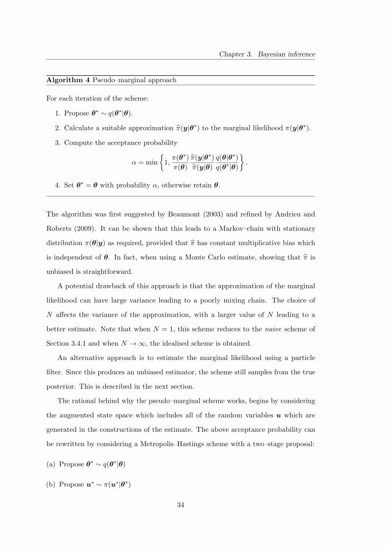
Algorithm 4 Pseudo–marginal approach
For each iteration of the scheme:
1. Propose θ∗ ∼ q(θ∗|θ).
2. Calculate a suitable approximation π(y|θ∗) to the marginal likelihood π(y|θ∗).
3. Compute the acceptance probability
α = min
{1,π(θ∗)
π(θ)
π(y|θ∗)π(y|θ)
q(θ|θ∗)q(θ∗|θ)
}.
4. Set θ∗ = θ with probability α, otherwise retain θ.
The algorithm was first suggested by Beaumont (2003) and refined by Andrieu and
Roberts (2009). It can be shown that this leads to a Markov–chain with stationary
distribution π(θ|y) as required, provided that π has constant multiplicative bias which
is independent of θ. In fact, when using a Monte Carlo estimate, showing that π is
unbiased is straightforward.
A potential drawback of this approach is that the approximation of the marginal
likelihood can have large variance leading to a poorly mixing chain. The choice of
N affects the variance of the approximation, with a larger value of N leading to a
better estimate. Note that when N = 1, this scheme reduces to the naive scheme of
Section 3.4.1 and when N →∞, the idealised scheme is obtained.
An alternative approach is to estimate the marginal likelihood using a particle
filter. Since this produces an unbiased estimator, the scheme still samples from the true
posterior. This is described in the next section.
The rational behind why the pseudo–marginal scheme works, begins by considering
the augmented state space which includes all of the random variables u which are
generated in the constructions of the estimate. The above acceptance probability can
be rewritten by considering a Metropolis–Hastings scheme with a two–stage proposal:
(a) Propose θ∗ ∼ q(θ∗|θ)
(b) Propose u∗ ∼ π(u∗|θ∗)
34

Chapter 3. Bayesian inference
and the acceptance probability becomes
α = min
{1,π(θ∗)
π(θ)
π(y|θ∗,u∗)π(y|θ,u)
π(u∗|θ∗)π(u|θ)
q(θ|θ∗)q(θ∗|θ)
π(u|θ)
π(u∗|θ∗)
}= min
{1,π(θ∗)
π(θ)
π(y|θ∗,u∗)π(y|θ,u)
q(θ|θ∗)q(θ∗|θ)
}.
It can be seen that the target distribution of this scheme is π(θ,u|y) and marginalising
over u gives
∫π(θ,u|y) du ∝
∫π(θ)π(y|θ,u)π(u|θ) du
∝ π(θ)
∫π(y|θ,u)π(u|θ) du
∝ π(θ)
∫Eu|θ(π(y|θ,u))
∝ π(θ)π(y|θ)
∝ π(θ|y).
The scheme is targeting a joint density with marginal π(θ|y), as required.
3.4.3 Particle filtering
A particle filter is a type of Sequential Monte Carlo (SMC) method which is a sequential
analogue of the MCMC techniques previously discussed. These techniques are particu-
larly useful for inference on state–space models which have a Markov structure. One
major advantage of SMC methods is that the analysis does not need to be restarted for
each new observation. This is particularly useful in applications where data arrive in
real time.
Suppose observations y1:T = (y1,y2, . . . ,yT ) are currently available, then the
posterior distribution of interest, assuming fixed θ, is
π(x1:T |y1:T ).
35

Chapter 3. Bayesian inference
If a new observation yT+1 becomes available, the posterior distribution of interest is
now π(xT+1|y1:T+1). Bayes’ Theorem can be used to incorporate this new observation
by updating the posterior distribution
π(xT+1|y1:T+1) ∝ π(xT+1|y1:T )π(yT+1|xT+1)
= π(yT+1|xT+1)
∫π(xT+1|xT )π(xT |y1:T ) dxT .
Notice that the final term in the integral is the posterior distribution at time T .
A particle filter can be used to target π(xT+1|y1:T+1). Before introducing particle
filters it is necessary to be familiar with the concept of importance resampling, which is
typically used in the implementation of the particle filtering algorithm.
Importance sampling and resampling
Importance resampling uses the principles of importance sampling: a technique for
performing Monte Carlo integration. Suppose the integral of interest is
I =
∫f(x)g(x) dx.
Assume it is not possible to sample from g(x), but it is possible to sample from a
different distribution q(x) which has the same support as g(x). Now multiply the
numerator and denominator by q(x)
I =
∫f(x)g(x)
q(x)
q(x)dx =
∫f(x)g(x)
q(x)× q(x) dx.
Suppose a sample x1, . . . ,xN is drawn from q(x), then a Monte Carlo estimate of I can
be constructed where
I =
N∑i=1
f(xi)g(xi)
q(xi).
36
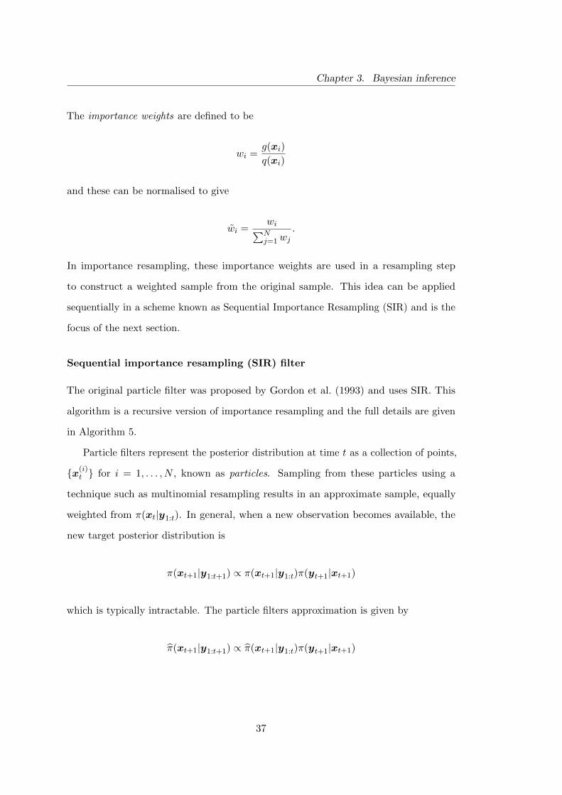
Chapter 3. Bayesian inference
The importance weights are defined to be
wi =g(xi)
q(xi)
and these can be normalised to give
wi =wi∑Nj=1wj
.
In importance resampling, these importance weights are used in a resampling step
to construct a weighted sample from the original sample. This idea can be applied
sequentially in a scheme known as Sequential Importance Resampling (SIR) and is the
focus of the next section.
Sequential importance resampling (SIR) filter
The original particle filter was proposed by Gordon et al. (1993) and uses SIR. This
algorithm is a recursive version of importance resampling and the full details are given
in Algorithm 5.
Particle filters represent the posterior distribution at time t as a collection of points,
{x(i)t } for i = 1, . . . , N , known as particles. Sampling from these particles using a
technique such as multinomial resampling results in an approximate sample, equally
weighted from π(xt|y1:t). In general, when a new observation becomes available, the
new target posterior distribution is
π(xt+1|y1:t+1) ∝ π(xt+1|y1:t)π(yt+1|xt+1)
which is typically intractable. The particle filters approximation is given by
π(xt+1|y1:t+1) ∝ π(xt+1|y1:t)π(yt+1|xt+1)
37

Chapter 3. Bayesian inference
Algorithm 5 Sequential importance resampling (SIR) filter
For time t = 1, . . . , T
For each particle {x(i)t }Ni=1
1. Simulate x(i)t+1 from π(xt+1|x(i)
t ).
2. Calculate importance weights
wi =π(yt+1|x
(i)t+1)∑N
j=1 π(yt+1|x(j)t+1)
.
3. Resample N times with replacement from the particles {x(i)t }Ni=1 using weights
{wi}Ni=1.
where
π(xt+1|y1:t) =1
N
N∑i=1
π(xt+1|x(i)
t
).
It is possible to sample from π(xt+1|y1:t), by first taking the sample of particles
approximately distributed according to π(xt|y1:t) and propagating forward. This is done
by forward simulating from the model i.e. using the Gillespie algorithm with parameters
θ and initial conditions x(i)t .
Using the principles of importance resampling, the importance weights are π(yt+1|x(i)t+1)
and the normalised weights are given by
wi =π(yt+1|x
(i)t+1)∑N
j=1 π(yt+1|x(j)t+1)
.
To generate an approximate, equally weighted sample from π(xt+1|y1:t+1), the particles
{x(i)t+1} must be resampled such that they are weighted by the importance weights wi.
The full algorithm is given in Algorithm 5 and is initialised by drawing an equally
weighted sample of particles {x(i)1 } from the prior distribution.
3.4.4 Application to pseudo–marginal approach
The particle marginal Metropolis-Hastings (PMMH) scheme of Andrieu et al. (2009, 2010)
creates an SMC approximation to the marginal likelihood π(y|x,θ). At each iteration
38

Chapter 3. Bayesian inference
of the MCMC scheme, the approximation is constructed by running a sequential scheme
such as the SIR filter (Algorithm 5). This scheme targets the posterior distribution of
the parameters and the latent states π(x,θ|y).
A special case of the PMMH scheme is where the marginal posterior π(θ|y) is
targeted. In this case, the estimate of the marginal likelihood is constructed by noting
that the average weight at time t gives an estimate of π(yt+1|y1:t,θ),
π(yt+1|y1:t,θ) =1
N
N∑j=1
π(yt+1|x(j)t+1,θ),
which is the marginal likelihood given data up to time t. An estimate of the marginal
likelihood given all data is the product of the average unnormalised weights
π(y|θ) =T−1∏t=0
1
N
N∑j=1
π(yt+1|x(j)t+1,θ)
. (3.3)
It is shown by Del Moral (2004) that Equation 3.3 provides a consistent and unbiased
estimate of the marginal likelihood. Given this property, a pseudo–marginal approach
can be used with Equation 3.3 as an estimate of the marginal likelihood in Algorithm 4.
This scheme also reduces to the naive scheme in Section 3.4.1 when N = 1. Andrieu
and Roberts (2009) note as the variance of the estimate of the marginal likelihood
decreases, the mixing improves. The more particles used, the lower the variance of
the estimate of marginal likelihood. Pitt et al. (2012) give guidelines on choosing the
number of particles, they suggest that N should be chosen such that the variance of the
log–posterior is 0.8464, although they suggest that anywhere in the range 0.25 - 2.25
will give only a small penalty. Doucet et al. (2012) suggest that the optimal value is
approximately 1. ?
3.4.5 Algorithm performance
When deciding to implement one of the methods for inference presented in this chapter,
the efficiency of the scheme is of major importance. One method of quantifying the
39
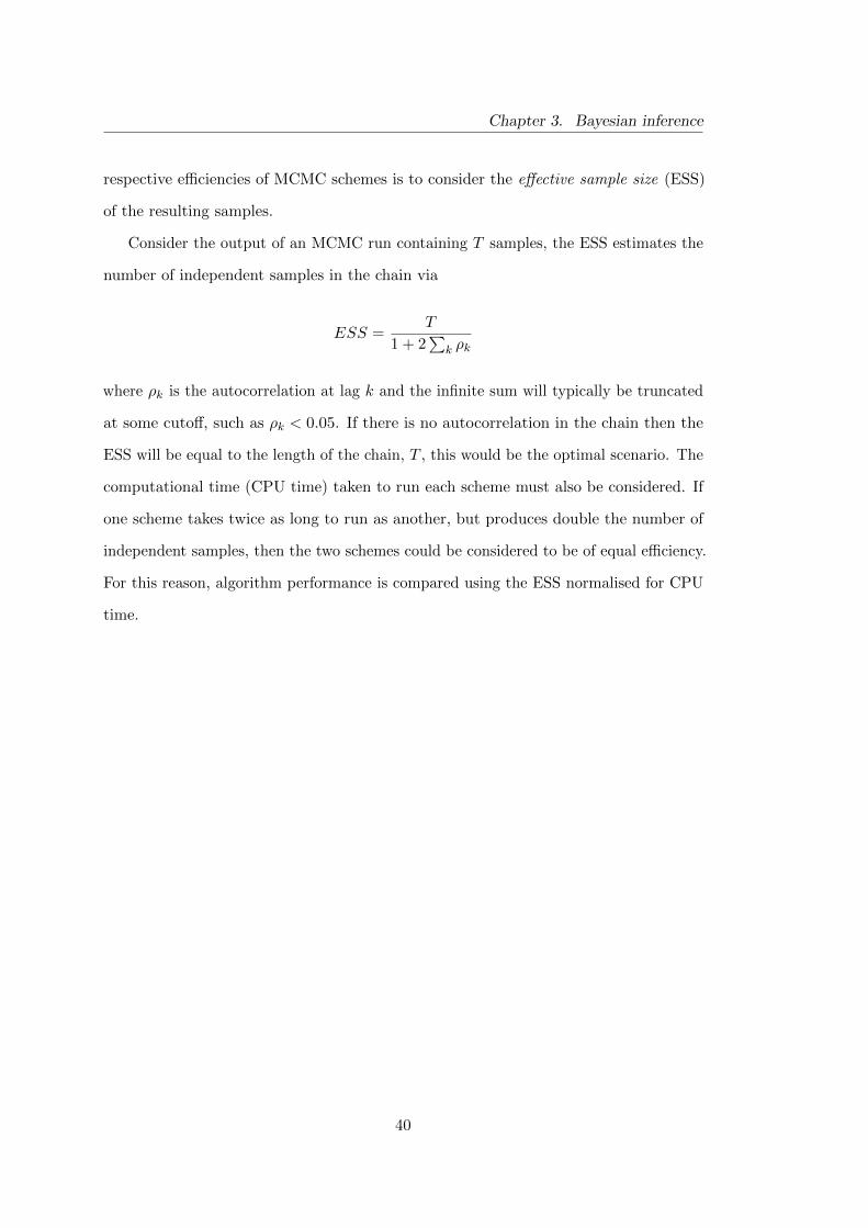
Chapter 3. Bayesian inference
respective efficiencies of MCMC schemes is to consider the effective sample size (ESS)
of the resulting samples.
Consider the output of an MCMC run containing T samples, the ESS estimates the
number of independent samples in the chain via
ESS =T
1 + 2∑
k ρk
where ρk is the autocorrelation at lag k and the infinite sum will typically be truncated
at some cutoff, such as ρk < 0.05. If there is no autocorrelation in the chain then the
ESS will be equal to the length of the chain, T , this would be the optimal scenario. The
computational time (CPU time) taken to run each scheme must also be considered. If
one scheme takes twice as long to run as another, but produces double the number of
independent samples, then the two schemes could be considered to be of equal efficiency.
For this reason, algorithm performance is compared using the ESS normalised for CPU
time.
40

Chapter 4
Numerical examples
This chapter considers two toy models, a model with no time dependence (constant
model) and the birth–death process. These models will be used to illustrate the methods
for inference outlined in Chapter 3. The advantage of testing methods on toy models
before looking at more complicated models is that they are quick to simulate from and
easier to work with. There are also certain analytic results which can be derived for
these models, which are not available in larger models. This property can be exploited to
compare approximate results to exact results, hence assess the performance of methods.
4.1 Constant model
Consider observed data y = (y1, y2, . . . , yT )T which are noisy proportions of cell death.
The data have no time dependence; they represent a discretely observed, noisy version
of a constant. When modelling proportions, a sensible choice is to work with the logit
transformed data
logitx = log
(x
1− x
),
which take values in R. Let µ = logit θ and assume the data model
yi ≡ logitxi = µ+ εi i = 1, . . . , T
41

Chapter 4. Numerical examples
where the εi are independent, εi ∼ N(0, 1/τ) and (µ, τ) are fixed but unknown parameters
of interest. Note, in this section, the measurement error is defined via the precision
τ = 1/σ2. While the error structure is normal on the logit scale, this translates to a
logistic–normal distribution on the original scale. There exists no analytic solutions
for the mean and variance of the logistic–normal distribution, see Aitchison (1986) for
details.
The aim is to make inferences on (µ, τ) given observed data y. This information is
summarised by the posterior distribution
π(µ, τ |y) ∝ π(µ)π(τ)π(y|µ, τ)
where
π(y|µ, τ) =T∏i=1
π(yi|µ, τ).
The likelihood is
π(y|µ, τ) =( τ
2π
)n/2exp
{−nτ
2[s2 + (y − µ)2]
}
where
s2 =1
n
n∑i=1
(yi − y)2.
Suppose a priori, beliefs about (µ, τ) are
µ ∼ N(b,
1
c
), e < µ < f and τ ∼ Γ (g, h), τ < k (4.1)
where b, c, e, f , g, h and k are known constants, and µ and τ are independent. Here,
the general case is considered, whereby prior beliefs may dictate that truncating either
42
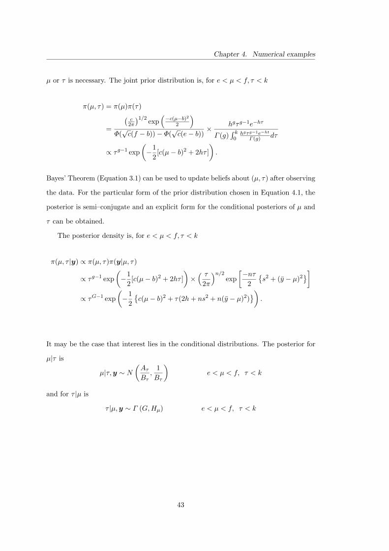
Chapter 4. Numerical examples
µ or τ is necessary. The joint prior distribution is, for e < µ < f, τ < k
π(µ, τ) = π(µ)π(τ)
=
(c2π
)1/2exp
(−c(µ−b)2
2
)Φ(√c(f − b))− Φ(
√c(e− b))
× hgτ g−1e−hτ
Γ (g)∫ k0hgτg−1e−ht
Γ (g) dτ
∝ τ g−1 exp
(−1
2[c(µ− b)2 + 2hτ ]
).
Bayes’ Theorem (Equation 3.1) can be used to update beliefs about (µ, τ) after observing
the data. For the particular form of the prior distribution chosen in Equation 4.1, the
posterior is semi–conjugate and an explicit form for the conditional posteriors of µ and
τ can be obtained.
The posterior density is, for e < µ < f, τ < k
π(µ, τ |y) ∝ π(µ, τ)π(y|µ, τ)
∝ τ g−1 exp
(−1
2[c(µ− b)2 + 2hτ ]
)×( τ
2π
)n/2exp
[−nτ
2
{s2 + (y − µ)2
}]∝ τG−1 exp
(−1
2
{c(µ− b)2 + τ(2h+ ns2 + n(y − µ)2)
}).
It may be the case that interest lies in the conditional distributions. The posterior for
µ|τ is
µ|τ,y ∼ N(AτBτ
,1
Bτ
)e < µ < f, τ < k
and for τ |µ is
τ |µ,y ∼ Γ (G,Hµ) e < µ < f, τ < k
43

Chapter 4. Numerical examples
where
Aτ = cb+ nyτ, Bτ = c+ nτ
G = g +n
2, Hµ = h+
n(y − µ)2
2+ns2
2.
Interest may also lie in marginal posterior distributions. The marginal posterior for τ
is, where τ < k,
π(τ |y) =
∫ f
eπ(µ, τ |y) dµ
∝∫ f
eτG−1 exp
(−1
2
{c(µ− b)2 + τ(2h+ ns2 + n(y − µ)2)
})dµ
∝ τG−1√Bτ
exp
(−1
2
{τ(2h+ ns2 + ny2)− A2
τ
Bτ
})[Φ
(√Bτ
(f − Aτ
Bτ
))− Φ
(√Bτ
(e− Aτ
Bτ
))]
and for µ is, where e < µ < f ,
π(µ|y) =
∫ k
0π(µ, τ |y) dτ
∝∫ k
0τG−1 exp
(−1
2
{c(µ− b)2 + τ(2h+ ns2 + n(y − µ)2)
})dτ
∝ exp
(−c(µ− b)
2
2
)H−Gµ G(k|G,Hµ)
where G(x|a, b) = Pr(Γ (a, b) ≤ x).
The marginal posterior distributions for µ and τ are only known up to a constant
of proportionality. However, a numerical integration technique such as the composite
trapezoidal rule can be used to find this constant. For simulated data and particular
choices of the prior parameters, marginal posterior distributions are given in the bottom
plot of Figure 4.1 (dashed line).
44
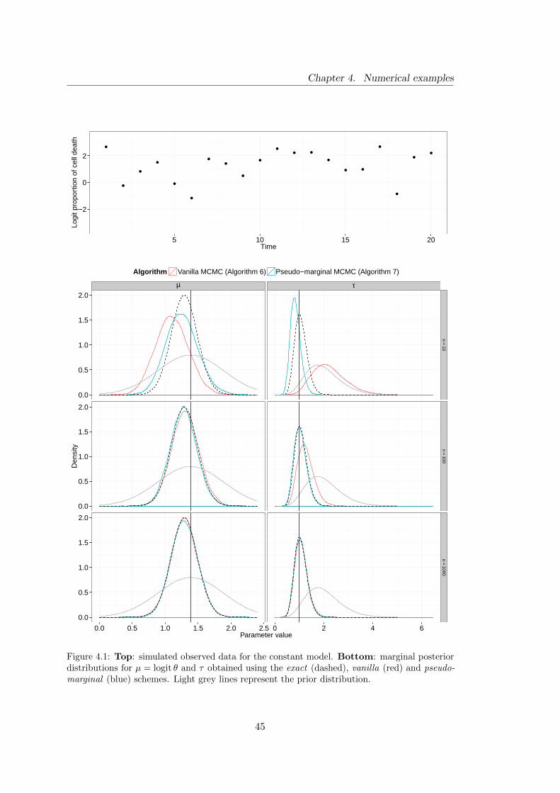
Chapter 4. Numerical examples
●
●
●
●
●
●
●
●
●
●
●
● ●
●
● ●
●
●
●
●
−2
0
2
5 10 15 20Time
Logi
t pro
port
ion
of c
ell d
eath
µ τ
0.0
0.5
1.0
1.5
2.0
0.0
0.5
1.0
1.5
2.0
0.0
0.5
1.0
1.5
2.0
n=
10n
=100
n=
1000
0.0 0.5 1.0 1.5 2.0 2.5 0 2 4 6Parameter value
Den
sity
Algorithm Vanilla MCMC (Algorithm 6) Pseudo−marginal MCMC (Algorithm 7)
Figure 4.1: Top: simulated observed data for the constant model. Bottom: marginal posteriordistributions for µ = logit θ and τ obtained using the exact (dashed), vanilla (red) and pseudo-marginal (blue) schemes. Light grey lines represent the prior distribution.
45

Chapter 4. Numerical examples
4.1.1 Constant model (with approximation)
Suppose the data model is now
yi = logitxi = logit p(θ) + εi i = 1, . . . , T (independent)
where the εi are independent, εi ∼ N(0, 1/τ) and (θ, τ) are fixed but unknown parameters
of interest. The probability of cell death p(θ) is now a function of θ. It is important to
consider this artificial scenario since it mimics the situation which arises when a more
complicated model underpins the cell death process and it is not possible to find an
analytic expression for the probability of cell death for given θ.
Of interest is inference on (θ, τ) where the posterior distribution is
π(θ, τ |y) ∝ π(θ)π(τ)π(y|θ, τ)
where
π(y|θ, τ) =T∏i=1
π(yi|θ, τ).
The p(θ) = [p1(θ), p2(θ), . . . , pT (θ)]T are unobserved latent states which can be approxi-
mated for any given θ by making T independent draws from the binomial distribution,
npi,n|p ∼ Bin[n, p(θ)] i = 1, . . . , T.
The simulated latent states are denoted
pn(θ) = [p1,n(θ), p2,n(θ), . . . , pT,n(θ)]T ,
where the n subscript describes how many independent draws from the Bernoulli
distribution were used to obtain the approximation. The quality of this approximation
depends on the value of n chosen. For small n, the approximation will be poor and
as n → ∞, the approximation tends towards the true proportion. Note, in a more
46

Chapter 4. Numerical examples
Algorithm 6 Constant model: inference using the vanilla scheme
Initialise the iteration counter and the state of the chain (θ, τ).
For each iteration of the scheme:
1. Sample (θ∗, τ∗) ∼ q(·|θ, τ) from a symmetric proposal distribution q, on the logscale.
2. Simulate the path p∗n(θ∗) for some choice of n.
3. Compute the acceptance probability
α = min
{1,π(θ∗)
π(θ)
π(τ∗)
π(τ)
π(y|θ∗, τ∗)π(y|θ, τ)
θ∗
θ
τ∗
τ
}.
4. Set (θ, τ) = (θ∗, τ∗) with probability α, otherwise retain (θ, τ).
complicated model where p(θ) is unobserved, the pn(θ) would be generated using n
forward simulations from the model.
Algorithms 6 and 7 present two schemes for inference on (θ, τ). These are MCMC
schemes which are based on the Metropolis-Hastings algorithm outlined in Algorithm 2
of Chapter 3. In both schemes, values of (θ∗, τ∗) are drawn from a symmetric proposal
distribution and used to simulate a realisation pn(θ∗). To calculate the marginal
likelihood for the data, it is necessary to marginalise over the simulated unobserved
latent states
π(y|θ, τ) '∫π(y|pn, τ)π(pn|θ) dpn
Also, as the components of pn have independent normal measurement errors, its joint
density can be written as
π(pn|θ) =
T∏i=1
π(pi,n|θ). (4.2)
Note that Algorithm 6 uses the normal approximation to the distribution of the empirical
logit of the pn where
elogit pi,n(θ) = log
(npi,n(θ) + 1/2
n− npi,n(θ) + 1/2
)i = 1, . . . , T
47

Chapter 4. Numerical examples
Algorithm 7 Constant model: inference using the pseudo-marginal scheme
Initialise the iteration counter and the state of the chain (θ, τ).
For each iteration of the scheme:
1. Sample (θ∗, τ∗) ∼ q(·|θ, τ) from a symmetric proposal distribution q, on the logscale.
2. For each particle 1, . . . , N , simulate a path p(1)n (θ∗), p(2)n (θ∗), . . . , p(N)n (θ∗) for some
choice of n.
3. Construct a Monte Carlo, unbiased estimate of π(y|θ∗, τ∗)
π(y|θ∗, τ∗) =1
N
N∑j=1
π(y|p(j)n (θ∗), τ∗)
where
π(y|p(j)n (θ∗), τ∗) =T∏i=1
π(yt|p(j)i,n(θ∗), τ∗)
4. Compute the acceptance probability
α = min
{1,π(θ∗)
π(θ)
π(τ∗)
π(τ)
π(y|θ∗, τ∗)π(y|θ, τ)
θ∗
θ
τ∗
τ
}.
5. Set (θ, τ) = (θ∗, τ∗) with probability α, otherwise retain (θ, τ).
and, for large n
elogit pi,n|θ ∼ N(
logit pi,n,1
npi,n[1− pi,n]
). (4.3)
This result can be shown as follows. Suppose pn is the proportion of successes out of
n independent trials. Then np|p ∼ Bin(n, p) and let npn = np+√np(1− p)Un, with
E(Un) = 0, V ar(Un) = 1, E(U2n) = 1. Also, Un → N(0, 1) as n→∞. Now
npn + 12
n− npn + 12
=np+
√np(1− p)Un + 1
2
n− np−√np(1− p)Un + 1
2
=p
1− p×
1 +
√(1− p)np
Un +1
2np
1−√
p
n(1− p)Un +
1
2n(1− p)
48

Chapter 4. Numerical examples
and so
elogit pn = log
(npn + 1
2
n− npn + 12
)
= logit p+ log
(1 +
√(1− p)np
Un +1
2np
)− log
(1−
√p
n(1− p)Un +
1
2n(1− p)
)
= logit p+
√(1− p)np
Un +1
2np− (1− p)
2npU2n
−{−√
p
n(1− p)Un +
1
2n(1− p)− p
n(1− p)U2n
}+O(n−3/2)
= logit p+Un√
p(1− p)n−1/2 +
(1− 2p)(1− U2n)
2p(1− p)n−1 +O(n−3/2).
Therefore
E(elogit pn) = logit p+O(n−3/2) and V ar(elogit pn) =1
np(1− p)+O(n−3/2).
Also, as Un → N(0, 1) as n→∞, for large n
elogit pn ∼ N(
logit p,1
np(1− p)
)approximately.
The scheme in Algorithm 6 will be referred to as the vanilla scheme throughout.
For the vanilla scheme, the marginal likelihood is evaluated directly using the results in
Equation 4.3 and 4.2. Since this result is approximate, this scheme is not exact and the
success of the scheme depends on the strength of the approximation in Equation 4.3.
Algorithm 7 is a pseudo-marginal scheme and is based on Algorithm 4 of Chapter 3.
At each iteration of the scheme, N realisations (particles) of the pn are simulated
p(1)n (θ∗)
...
p(j)n (θ∗)
...
p(N)n (θ∗)
=
p(1)t1,n
(θ∗) . . . p(1)ti,n
(θ∗) . . . p(1)tT ,n
(θ∗)
......
...
p(i)t1,n
(θ∗) . . . p(i)ti,n
(θ∗) . . . p(i)tT ,n
(θ∗)
......
...
p(N)t1,n
(θ∗) . . . p(N)ti,n
(θ∗) . . . p(N)tT ,n
(θ∗)
.
49

Chapter 4. Numerical examples
These particles are used to construct an unbiased estimate of the marginal likelihood
π(y|θ, τ) =1
N
N∑j=1
π(y|p(j)n , τ).
This estimate of the marginal likelihood is used in place of π(y|θ, τ) in the acceptance
ratio and since approximation is unbiased, the exact posterior is targeted.
For the vanilla scheme, at each iteration T draws from the binomial distribution are
required, one for each data point. In the pseudo-marginal scheme, N × T draws are
required from the binomial distribution for each iteration of the scheme. For this model,
the simulation strategy is very simple and quick. However, a more complex model will
be slower to simulate from; hence, keeping the number of simulations to a minimum
will be of greater importance.
4.1.2 Constant model: results
Data were simulated from the model with θ = 0.8, τ = 1 and T = 20; the data are
presented in the top plot of Figure 4.1 (page 45). The results of inference on this data
using Algorithms 6 and 7 with prior distributions
µ = logit θ ∼ N(
logit 0.8,1
4
)0 < µ < 5 and τ ∼ Γ (8, 4) τ < 10
can be seen in the bottom plot.
The exact marginal posterior distributions of µ = logit θ and τ can both be obtained
up to a constant of proportionality using the expressions calculated in Section 4.1.
Numerical integration was used to obtain these constants. These marginal posterior
distributions are shown in dotted lines in Figure 4.1 and will be known as the exact
case; also shown are the results of running Algorithms 6 and 7 for different choices of n.
The performance of the algorithms can be assessed informally by observing how
close the resulting posterior distributions are to the exact case in Figure 4.1. Firstly, it
can be noted that as n increases, both the vanilla and pseudo-marginal schemes become
50

Chapter 4. Numerical examples
indistinguishable from the exact case, this happens when n ≥ 1000. The pseudo-marginal
approach seems to do better than the vanilla approach, especially when n is small. This
is as expected, since the approximation used in the vanilla approach (Equation 4.3) is
dependent on n being large.
4.2 Birth–death model
The simple birth–death process was introduced in Chapter 2. The model is more
complex than the constant model, although it is still possible to obtain an analytic
expression for the transition probabilities. The chemical master equations (CME) is
dPx(t)
dt= λ(x− 1)Px−1(t) + µ(x+ 1)Px+1(t)− x(λ+ µ)Px(t). (4.4)
This probability generating function is given by
Q(z; t) =
∞∑x=0
Px(t)zx
and it follows that
∂
∂tQ(z; t) =
∞∑x=0
∂
∂tPx(t)zx. (4.5)
Equation 4.4 can be written in terms of the probability generating function by multiplying
both sides by zx and summing over x, giving
∂
∂t
∞∑x=0
zxPx(t) =∞∑x=0
zx {λ(x− 1)Px−1(t) + µ(x+ 1)Px+1(t)− x(λ+ µ)Px(t)}
which satisfies the partial differential equation (p.d.e.)
∂Q
∂t= (λz − µ)(z − 1)
∂Q
∂z.
51
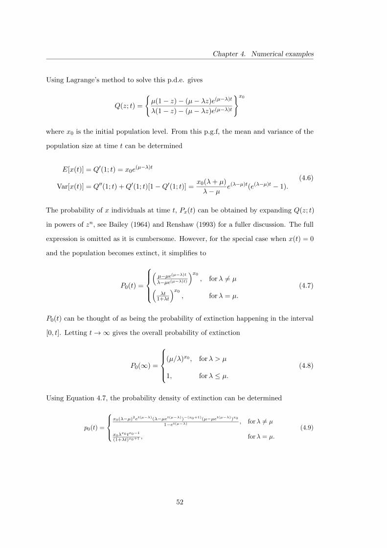
Chapter 4. Numerical examples
Using Lagrange’s method to solve this p.d.e. gives
Q(z; t) =
{µ(1− z)− (µ− λz)e(µ−λ)t
λ(1− z)− (µ− λz)e(µ−λ)t
}x0
where x0 is the initial population level. From this p.g.f, the mean and variance of the
population size at time t can be determined
E[x(t)] = Q′(1; t) = x0e(µ−λ)t
Var[x(t)] = Q′′(1; t) +Q′(1; t)[1−Q′(1; t)] =x0(λ+ µ)
λ− µe(λ−µ)t(e(λ−µ)t − 1).
(4.6)
The probability of x individuals at time t, Px(t) can be obtained by expanding Q(z; t)
in powers of zn, see Bailey (1964) and Renshaw (1993) for a fuller discussion. The full
expression is omitted as it is cumbersome. However, for the special case when x(t) = 0
and the population becomes extinct, it simplifies to
P0(t) =
(µ−µe(µ−λ)tλ−µe(µ−λ)t)
)x0, forλ 6= µ(
λt1+λt
)x0, forλ = µ.
(4.7)
P0(t) can be thought of as being the probability of extinction happening in the interval
[0, t]. Letting t→∞ gives the overall probability of extinction
P0(∞) =
(µ/λ)x0 , forλ > µ
1, forλ ≤ µ.(4.8)
Using Equation 4.7, the probability density of extinction can be determined
p0(t) =
x0(λ−µ)2et(µ−λ)(λ−µet(µ−λ))−(x0+1)(µ−µet(µ−λ))x0
1−et(µ−λ) , forλ 6= µ
x0λx0 tx0−1
(1+λt)x0+1 , forλ = µ.
(4.9)
52

Chapter 4. Numerical examples
0
5
10
15
0.0 2.5 5.0 7.5 10.0Time
Pop
ulat
ion
leve
l (X
)
Figure 4.2: Three simulations of the birth–death process with λ = 0.6, µ = 1 and x0 = 10 alongwith the mean (black line).
4.2.1 Simulating from the model
The time evolution of a population governed by a birth–death process (with a particular
choice of λ, µ and x0) can be simulated using a stochastic simulation algorithm such as
the Gillespie algorithm (see Algorithm 1 of Chapter 2). Since the model is stochastic,
each simulation will be different; this is illustrated in Figure 4.2 where three typical
trajectories are shown along with the mean (given in Equation 4.6).
A set of extinction times could be obtained by simulating the trajectories of several
populations and recording the times at which they became extinct. However, since the
cumulative distribution function (c.d.f.) for extinction times (Equation 4.7) is known
and invertible, the inversion sampling method provides a more convenient method of
doing this. To simulate a time of extinction, t:
53

Chapter 4. Numerical examples
1. Calculate the overall probability of extinction
P0(∞) =
(µ/λ)x0 , forλ > µ
1, forλ ≤ µ.
2. Generate a realisation u ∼ U(0, 1).
3. If u < P0(∞), compute
t =
1
µ−λ log(λu1/x0−µµu1/x0−µ
), forλ 6= µ
u1/x0
λ(1−u1/x0 ) , forλ = µ,
otherwise t =∞.
Simulating n populations each governed by a birth–death process and noting when
each population becomes extinct gives an estimate of the proportion of extinction through
time. An example of this can be seen in Figure 4.3. In this plot, the green line is the
exact proportion of extinction through time. The other lines represents the approximate
proportion of extinction gained from using a simulator with n = (10, 102, 103, 104). For
low n, the approximation is very poor, however, when n = 104, the simulator output is
virtually indistinguishable from the exact values.
In the subsequent sections, inference is described for data in which the underlying
process is a birth–death process. Several situations for how the data are observed
are discussed. In each scenario, it is assumed that there are several populations each
governed by a birth–death process. In Section 4.2.2 is it assumed that the extinction
time for each population is observed exactly. Section 4.2.3 assumes that extinction times
are observed at discrete intervals, this represents a more plausible real life scenario. Of
interest is the impact on the amount information learnt when data are observed on
a finer grid. Section 4.2.4 considers the case in which the number of extinctions are
observed with noise, thus the true proportions are unobserved latent states.
The MCMC schemes for inference are described in detail in Algorithms 8–12. For
54
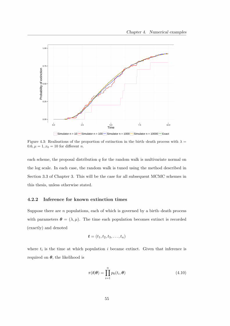
Chapter 4. Numerical examples
0.00
0.25
0.50
0.75
1.00
0.0 2.5 5.0 7.5 10.0
Time
Pro
babi
lity
of e
xtin
ctio
n
Simulator n = 10 Simulator n = 100 Simulator n = 1000 Simulator n = 10000 Exact
Figure 4.3: Realisations of the proportion of extinction in the birth–death process with λ =0.6, µ = 1, x0 = 10 for different n.
each scheme, the proposal distribution q for the random walk is multivariate normal on
the log scale. In each case, the random walk is tuned using the method described in
Section 3.3 of Chapter 3. This will be the case for all subsequent MCMC schemes in
this thesis, unless otherwise stated.
4.2.2 Inference for known extinction times
Suppose there are n populations, each of which is governed by a birth–death process
with parameters θ = (λ, µ). The time each population becomes extinct is recorded
(exactly) and denoted
t = (t1, t2, t3, . . . , tn)
where ti is the time at which population i became extinct. Given that inference is
required on θ, the likelihood is
π(t|θ) =
n∏i=1
p0(ti,θ) (4.10)
55

Chapter 4. Numerical examples
Algorithm 8 Birth–death model: inference using known extinction times
Initialise the iteration counter and the state of the chain θ.
For each iteration of the scheme:
1. Sample θ∗ ∼ q(·|θ) from a symmetric proposal distribution q, on the log scale.
2. Compute the acceptance probability
α = min
{1,π(θ∗)
π(θ)
n∏i=1
p0(ti,θ∗)
p0(ti,θ)
p∏i=1
θ∗iθi
}.
3. Set θ = θ∗ with probability α, otherwise retain θ.
where p0 is given in Equation 4.9. The posterior distribution of interest is
π(θ|t) ∝ π(θ)π(t|θ) (4.11)
where π(θ) is the prior distribution for θ.
Implementation
It was assumed a priori that x0 = 10, λ and µ were independent and
λ ∼ Log-Normal(log 0.6, 2) and µ ∼ Log-Normal(log 1, 2). (4.12)
These posterior distributions were chosen to represent vague prior information about
parameters. The posterior distribution π(θ|t) does not have recognisable form but can
be targeted with an MCMC scheme outlined in Algorithm 8. This scheme is based on
the Metropolis-Hastings scheme which was first introduced in Chapter 3 (Algorithm 2).
Three different datasets t were simulated using the algorithm in Section 4.2.1 and
using n = (10, 100, 1000) forward simulations from the model, each with λ = 0.6 and
µ = 1. Inference was performed for each dataset using Algorithm 8.
The marginal posterior distributions (pink) along with the joint posterior (blue) are
shown in Figure 4.4, where each row corresponds to a different dataset. It appears that
56

Chapter 4. Numerical examples
●●●●●●●●●●●●●●●●●●●●●●●●●●●●●●●●●●●●●●●●●●●●●●●●●●●●●●●●●●●●●●●●●●●●●●●●●●●●●●●●●●●●●●●●●●●●●●●●●●●●●●●●●●●●●●●●●●●●●●●●●●●●●●●●●●●●●●●●●●●●●●●●●●●●●●●●●●●●●●●●●●●●●●●●●●●●●●●●●●●●●●●●●●●●●●●●●●●●●●●●●●●●●●●●●●●●●●●●●●●●●●●●●●●●●●●●●●●●●●●●●●●●●●●●●●●●●●●●●●●●●●●●●●●●●●●●●●●●●●●●●●●●●●●●●●●●●●●●●●●●●●●●●●●●●●●●●●●●●●●●●●●●●●●●●●●●●●●●●●●●●●●●●●●●●●●●●●●●●●●●●●●●●●●●●●●●●●●●●●●●●●●●●●●●●●●●●●●●●●●●●●●●●●●●●●●●●●●●●●●●●●●●●●●●●●●●●●●●●●●●●●●●●●●●●●●●●●●●●●●●●●●●●●●●●●●●●●●●●●●●●●●●●●●●●●●●●●●●●●●●●●●●●●●●●●●●●●●●●●●●●●●●●●●●●●●●●●●●●●●●●●●●●●●●●●●●●●●●●●●●●●●●●●●●●●●●●●●●●●●●●●●●●●●●●●●●●●●●●●●●●●●●●●●●●●●●●●●●●●●●●●●●●●●●●●●●●●●●●●●●●●●●●●●●●●●●●●●●●●●●●●●●●●●●●●●●●●●●●●●●●●●●●●●●●●●●●●●●●●●●●●●●●●●●●●●●●●●●●●●●●●●●●●●●●●●●●●●●●●●●●●●●●●●●●●●●●●●●●●●●●●●●●●●●●●●●●●●●●●●●●●●●●●●●●●●●●●●●●●●●●●●●●●●●●●●●●●●●●●●●●●●●●●●●●●●●●●●●●●●●●●●●●●●●●●●●●●●●●●●●●●●●●●●●●●●●●●●●●●●●●●●●●●●●●●●●●●●●●●●●●●●●●●●●●●●●●●●●●●●●●●●●●●●●●●●●●●●●●●●●●●●●●●●●●●●●●●●●●●●●●●●●●●●●●●●●●●●●●●●●●●●●●●●●●●●●●●●●●●●●●●●●●●●●●●●●●●●●●●●●●●●●●●●●●●●●●●●●●●●●●●●●●●●●●●●●●●●●●●●●●●●●●●●●●●●●●●●●●●●●●●●●●●●●●●●●●●●●●●●●●●●●●●●●●●●●●●●●●●●●●●●●●●●●●●●●●●●●●●●●●●●●●●●●●●●●●●●●●●●●●●●●●●●●●●●●●●●●●●●●●●●●●●●●●●●●●●●●●●●●●●●●●●●●●●●●●●●●●●●●●●●●●●●●●●●●●●●●●●●●●●●●●●●●●●●●●●●●●●●●●●●●●●●●●●●●●●●●●●●●●●●●●●●●●●●●●●●●●●●●●●●●●●●●●●●●●●●●●●●●●●●●●●●●●●●●●●●●●●●●●●●●●●●●●●●●●●●●●●●●●●●●●●●●●●●●●●●●●●●●●●●●●●●●●●●●●●●●●●●●●●●●●●●●●●●●●●●●●●●●●●●●●●●●●●●●●●●●●●●●●●●●●●●●●●●●●●●●●●●●●●●●●●●●●●●●●●●●●●●●●●●●●●●●●●●●●●●●●●●●●●●●●●●●●●●●●●●●●●●●●●●●●●●●●●●●●●●●●●●●●●●●●●●●●●●●●●●●●●●●●●●●●●●●●●●●●●●●●●●●●●●●●●●●●●●●●●●●●●●●●●●●●●●●●●●●●●●●●●●●●●●●●●●●●●●●●●●●●●●●●●●●●●●●●●●●●●●●●●●●●●●●●●●●●●●●●●●●●●●●●●●●●●●●●●●●●●●●●●●●●●●●●●●●●●●●●●●●●●●●●●●●●●●●●●●●●●●●●●●●●●●●●●●●●●●●●●●●●●●●●●●●●●●●●●●●●●●●●●●●●●●●●●●●●●●●●●●●●●●●●●●●●●●●●●●●●●●●●●●●●●●●●●●●●●●●●●●●●●●●●●●●●●●●●●●●●●●●●●●●●●●●●●●●●●●●●●●●●●●●●●●●●●●●●●●●●●●●●●●●●●●●●●●●●●●●●●●●●●●●●●●●●●●●●●●●●●●●●●●●●●●●●●●●●●●●●●●●●●●●●●●●●●●●●●●●●●●●●●●●●●●●●●●●●●●●●●●●●●●●●●●●●●●●●●●●●●●●●●●●●●●●●●●●●●●●●●●●●●●●●●●●●●●●●●●●●●●●●●●●●●●●●●●●●●●●●●●●●●●●●●●●●●●●●●●●●●●●●●●●●●●●●●●●●●●●●●●●●●●●●●●●●●●●●●●●●●●●●●●●●●●●●●●●●●●●●●●●●●●●●●●●●●●●●●●●●●●●●●●●●●●●●●●●●●●●●●●●●●●●●●●●●●●●●●●●●●●●●●●●●●●●●●●●●●●●●●●●●●●●●●●●●●●●●●●●●●●●●●●●●●●●●●●●●●●●●●●●●●●●●●●●●●●●●●●●●●●●●●●●●●●●●●●●●●●●●●●●●●●●●●●●●●●●●●●●●●●●●●●●●●●●●●●●●●●●●●●●●●●●●●●●●●●●●●●●●●●●●●●●●●●●●●●●●●●●●●●●●●●●●●●●●●●●●●●●●●●●●●●●●●●●●●●●●●●●●●●●●●●●●●●●●●●●●●●●●●●●●●●●●●●●●●●●●●●●●●●●●●●●●●●●●●●●●●●●●●●●●●●●●●●●●●●●●●●●●●●●●●●●●●●●●●●●●●●●●●●●●●●●●●●●●●●●●●●●●●●●●●●●●●●●●●●●●●●●●●●●●●●●●●●●●●●●●●●●●●●●●●●●●●●●●●●●●●●●●●●●●●●●●●●●●●●●●●●●●●●●●●●●●●●●●●●●●●●●●●●●●●●●●●●●●●●●●●●●●●●●●●●●●●●●●●●●●●●●●●●●●●●●●●●●●●●●●●●●●●●●●●●●●●●●●●●●●●●●●●●●●●●●●●●●●●●●●●●●●●●●●●●●●●●●●●●●●●●●●●●●●●●●●●●●●●●●●●●●●●●●●●●●●●●●●●●●●●●●●●●●●●●●●●●●●●●●●●●●●●●●●●●●●●●●●●●●●●●●●●●●●●●●●●●●●●●●●●●●●●●●●●●●●●●●●●●●●●●●●●●●●●●●●●●●●●●●●●●●●●●●●●●●●●●●●●●●●●●●●●●●●●●●●●●●●●●●●●●●●●●●●●●●●●●●●●●●●●●●●●●●●●●●●●●●●●●●●●●●●●●●●●●●●●●●●●●●●●●●●●●●●●●●●●●●●●●●●●●●●●●●●●●●●●●●●●●●●●●●●●●●●●●●●●●●●●●●●●●●●●●●●●●●●●●●●●●●●●●●●●●●●●●●●●●●●●●●●●●●●●●●●●●●●●●●●●●●●●●●●●●●●●●●●●●●●●●●●●●●●●●●●●●●●●●●●●●●●●●●●●●●●●●●●●●●●●●●●●●●●●●●●●●●●●●●●●●●●●●●●●●●●●●●●●●●●●●●●●●●●●●●●●●●●●●●●●●●●●●●●●●●●●●●●●●●●●●●●●●●●●●●●●●●●●●●●●●●●●●●●●●●●●●●●●●●●●●●●●●●●●●●●●●●●●●●●●●●●●●●●●●●●●●●●●●●●●●●●●●●●●●●●●●●●●●●●●●●●●●●●●●●●●●●●●●●●●●●●●●●●●●●●●●●●●●●●●●●●●●●●●●●●●●●●●●●●●●●●●●●●●●●●●●●●●●●●●●●●●●●●●●●●●●●●●●●●●●●●●●●●●●●●●●●●●●●●●●●●●●●●●●●●●●●●●●●●●●●●●●●●●●●●●●●●●●●●●●●●●●●●●●●●●●●●●●●●●●●●●●●●●●●●●●●●●●●●●●●●●●●●●●●●●●●●●●●●●●●●●●●●●●●●●●●●●●●●●●●●●●●●●●●●●●●●●●●●●●●●●●●●●●●●●●●●●●●●●●●●●●●●●●●●●●●●●●●●●●●●●●●●●●●●●●●●●●●●●●●●●●●●●●●●●●●●●●●●●●●●●●●●●●●●●●●●●●●●●●●●●●●●●●●●●●●●●●●●●●●●●●●●●●●●●●●●●●●●●●●●●●●●●●●●●●●●●●●●●●●●●●●●●●●●●●●●●●●●●●●●●●●●●●●●●●●●●●●●●●●●●●●●●●●●●●●●●●●●●●●●●●●●●●●●●●●●●●●●●●●●●●●●●●●●●●●●●●●●●●●●●●●●●●●●●●●●●●●●●●●●●●●●●●●●●●●●●●●●●●●●●●●●●●●●●●●●●●●●●●●●●●●●●●●●●●●●●●●●●●●●●●●●●●●●●●●●●●●●●●●●●●●●●●●●●●●●●●●●●●●●●●●●●●●●●●●●●●●●●●●●●●●●●●●●●●●●●●●●●●●●●●●●●●●●●●●●●●●●●●●●●●●●●●●●●●●●●●●●●●●●●●●●●●●●●●●●●●●●●●●●●●●●●●●●●●●●●●●●●●●●●●●●●●●●●●●●●●●●●●●●●●●●●●●●●●●●●●●●●●●●●●●●●●●●●●●●●●●●●●●●●●●●●●●●●●●●●●●●●●●●●●●●●●●●●●●●●●●●●●●●●●●●●●●●●●●●●●●●●●●●●●●●●●●●●●●●●●●●●●●●●●●●●●●●●●●●●●●●●●●●●●●●●●●●●●●●●●●●●●●●●●●●●●●●●●●●●●●●●●●●●●●●●●●●●●●●●●●●●●●●●●●●●●●●●●●●●●●●●●●●●●●●●●●●●●●●●●●●●●●●●●●●●●●●●●●●●●●●●●●●●●●●●●●●●●●●●●●●●●●●●●●●●●●●●●●●●●●●●●●●●●●●●●●●●●●●●●●●●●●●●●●●●●●●●●●●●●●●●●●●●●●●●●●●●●●●●●●●●●●●●●●●●●●●●●●●●●●●●●●●●●●●●●●●●●●●●●●●●●●●●●●●●●●●●●●●●●●●●●●●●●●●●●●●●●●●●●●●●●●●●●●●●●●●●●●●●●●●●●●●●●●●●●●●●●●●●●●●●●●●●●●●●●●●●●●●●●●●●●●●●●●●●●●●●●●●●●●●●●●●●●●●●●●●●●●●●●●●●●●●●●●●●●●●●●●●●●●●●●●●●●●●●●●●●●●●●●●●●●●●●●●●●●●●●●●●●●●●●●●●●●●●●●●●●●●●●●●●●●●●●●●●●●●●●●●●●●●●●●●●●●●●●●●●●●●●●●●●●●●●●●●●●●●●●●●●●●●●●●●●●●●●●●●●●●●●●●●●●●●●●●●●●●●●●●●●●●●●●●●●●●●●●●●●●●●●●●●●●●●●●●●●●●●●●●●●●●●●●●●●●●●●●●●●●●●●●●●●●●●●●●●●●●●●●●●●●●●●●●●●●●●●●●●●●●●●●●●●●●●●●●●●●●●●●●●●●●●●●●●●●●●●●●●●●●●●●●●●●●●●●●●●●●●●●●●●●●●●●●●●●●●●●●●●●●●●●●●●●●●●●●●●●●●●●●●●●●●●●●●●●●●●●●●●●●●●●●●●●●●●●●●●●●●●●●●●●●●●●●●●●●●●●●●●●●●●●●●●●●●●●●●●●●●●●●●●●●●●●●●●●●●●●●●●●●●●●●●●●●●●●●●●●●●●●●●●●●●●●●●●●●●●●●●●●●●●●●●●●●●●●●●●●●●●●●●●●●●●●●●●●●●●●●●●●●●●●●●●●●●●●●●●●●●●●●●●●●●●●●●●●●●●●●●●●●●●●●●●●●●●●●●●●●●●●●●●●●●●●●●●●●●●●●●●●●●●●●●●●●●●●●●●●●●●●●●●●●●●●●●●●●●●●●●●●●●●●●●●●●●●●●●●●●●●●●●●●●●●●●●●●●●●●●●●●●●●●●●●●●●●●●●●●●●●●●●●●●●●●●●●●●●●●●●●●●●●●●●●●●●●●●●●●●●●●●●●●●●●●●●●●●●●●●●●●●●●●●●●●●●●●●●●●●●●●●●●●●●●●●●●●●●●●●●●●●●●●●●●●●●●●●●●●●●●●●●●●●●●●●●●●●●●●●●●●●●●●●●●●●●●●●●●●●●●●●●●●●●●●●●●●●●●●●●●●●●●●●●●●●●●●●●●●●●●●●●●●●●●●●●●●●●●●●●●●●●●●●●●●●●●●●●●●●●●●●●●●●●●●●●●●●●●●●●●●●●●●●●●●●●●●●●●●●●●●●●●●●●●●●●●●●●●●●●●●●●●●●●●●●●●●●●●●●●●●●●●●●●●●●●●●●●●●●●●●●●●●●●●●●●●●●●●●●●●●●●●●●●●●●●●●●●●●●●●●●●●●●●●●●●●●●●●●●●●●●●●●●●●●●●●●●●●●●●●●●●●●●●●●●●●●●●●●●●●●●●●●●●●●●●●●●●●●●●●●●●●●●●●●●●●●●●●●●●●●●●●●●●●●●●●●●●●●●●●●●●●●●●●●●●●●●●●●●●●●●●●●●●●●●●●●●●●●●●●●●●●●●●●●●●●●●●●●●●●●●●●●●●●●●●●●●●●●●●●●●●●●●●●●●●●●●●●●●●●●●●●●●●●●●●●●●●●●●●●●●●●●●●●●●●●●●●●●●●●●●●●●●●●●●●●●●●●●●●●●●●●●●●●●●●●●●●●●●●●●●●●●●●●●●●●●●●●●●●●●●●●●●●●●●●●●●●●●●●●●●●●●●●●●●●●●●●●●●●●●●●●●●●●●●●●●●●●●●●●●●●●●●●●●●●●●●●●●●●●●●●●●●●●●●●●●●●●●●●●●●●●●●●●●●●●●●●●●●●●●●●●●●●●●●●●●●●●●●●●●●●●●●●●●●●●●●●●●●●●●●●●●●●●●●●●●●●●●●●●●●●●●●●●●●●●●●●●●●●●●●●●●●●●●●●●●●●●●●●●●●●●●●●●●●●●●●●●●●●●●●●●●●●●●●●●●●●●●●●●●●●●●●●●●●●●●●●●●●●●●●●●●●●●●●●●●●●●●●●●●●●●●●●●●●●●●●●●●●●●●●●●●●●●●●●●●●●●●●●●●●●●●●●●●●●●●●●●●●●●●●●●●●●●●●●●●●●●●●●●●●●●●●●●●●●●●●●●●●●●●●●●●●●●●●●●●●●●●●●●●●●●●●●●●●●●●●●●●●●●●●●●●●●●●●●●●●●●●●●●●●●●●●●●●●●●●●●●●●●●●●●●●●●●●●●●●●●●●●●●●●●●●●●●●●●●●●●●●●●●●●●●●●●●●●●●●●●●●●●●●●●●●●●●●●●●●●●●●●●●●●●●●●●●●●●●●●●●●●●●●●●●●●●●●●●●●●●●●●●●●●●●●●●●●●●●●●●●●●●●●●●●●●●●●●●●●●●●●●●●●●●●●●●●●●●●●●●●●●●●●●●●●●●●●●●●●●●●●●●●●●●●●●●●●●●●●●●●●●●●●●●●●●●●●●●●●●●●●●●●●●●●●●●●●●●●●●●●●●●●●●●●●●●●●●●●●●●●●●●●●●●●●●●●●●●●●●●●●●●●●●●●●●●●●●●●●●●●●●●●●●●●●●●●●●●●●●●●●●●●●●●●●●●●●●●●●●●●●●●●●●●●●●●●●●●●●●●●●●●●●●●●●●●●●●●●●●●●●●●●●●●●●●●●●●●●●●●●●●●●●●●●●●●●●●●●●●●●●●●●●●●●●●●●●●●●●●●●●●●●●●●●●●●●●●●●●●●●●●●●●●●●●●●●●●●●●●●●●●●●●●●●●●●●●●●●●●●●●●●●●●●●●●●●●●●●●●●●●●●●●●●●●●●●●●●●●●●●●●●●●●●●●●●●●●●●●●●●●●●●●●●●●●●●●●●●●●●●●●●●●●●●●●●●●●●●●●●●●●●●●●●●●●●●●●●●●●●●●●●●●●●●●●●●●●●●●●●●●●●●●●●●●●●●●●●●●●●●●●●●●●●●●●●●●●●●●●●●●●●●●●●●●●●●●●●●●●●●●●●●●●●●●●●●●●●●●●●●●●●●●●●●●●●●●●●●●●●●●●●●●●●●●●●●●●●●●●●●●●●●●●●●●●●●●●●●●●●●●●●●●●●●●●●●●●●●●●●●●●●●●●●●●●●●●●●●●●●●●●●●●●●●●●●●●●●●●●●●●●●●●●●●●●●●●●●●●●●●●●●●●●●●●●●●●●●●●●●●●●●●●●●●●●●●●●●●●●●●●●●●●●●●●●●●●●●●●●●●●●●●●●●●●●●●●●●●●●●●●●●●●●●●●●●●●●●●●●●●●●●●●●●●●●●●●●●●●●●●●●●●●●●●●●●●●●●●●●●●●●●●●●●●●●●●●●●●●●●●●●●●●●●●●●●●●●●●●●●●●●●●●●●●●●●●●●●●●●●●●●●●●●●●●●●●●●●●●●●●●●●●●●●●●●●●●●●●●●●●●●●●●●●●●●●●●●●●●●●●●●●●●●●●●●●●●●●●●●●●●●●●●●●●●●●●●●●●●●●●●●●●●●●●●●●●●●●●●●●●●●●●●●●●●●●●●●●●●●●●●●●●●●●●●●●●●●●●●●●●●●●●●●●●●●●●●●●●●●●●●●●●●●●●●●●●●●●●●●●●●●●●●●●●●●●●●●●●●●●●●●●●●●●●●●●●●●●●●●●●●●●●●●●●●●●●●●●●●●●●●●●●●●●●●●●●●●●●●●●●●●●●●●●●●●●●●●●●●●●●●●●●●●●●●●●●●●●●●●●●●●●●●●●●●●●●●●●●●●●●●●●●●●●●●●●●●●●●●●●●●●●●●●●●●●●●●●●●●●●●●●●●●●●●●●●●●●●●●●●●●●●●●●●●●●●●●●●●●●●●●●●●●●●●●●●●●●●●●●●●●●●●●●●●●●●●●●●●●●●●●●●●●●●●●●●●●●●●●●●●●●●●●●●●●●●●●●●●●●●●●●●●●●●●●●●●●●●●●●●●●●●●●●●●●●●●●●●●●●●●●●●●●●●●●●●●●●●●●●●●●●●●●●●●●●●●●●●●●●●●●●●●●●●●●●●●●●●●●●●●●●●●●●●●●●●●●●●●●●●●●●●●●●●●●●●●●●●●●●●●●●●●●●●●●●●●●●●●●●●●●●●●●●●●●●●●●●●●●●●●●●●●●●●●●●●●●●●●●●●●●●●●●●●●●●●●●●●●●●●●●●●●●●●●●●●●●●●●●●●●●●●●●●●●●●●●●●●●●●●●●●●●●●●●●●●●●●●●●●●●●●●●●●●●●●●●●●●●●●●●●●●●●●●●●●●●●●●●●●●●●●●●●●●●●●●●●●●●●●●●●●●●●●●●●●●●●●●●●●●●●●●●●●●●●●●●●●●●●●●●●●●●●●●●●●●●●●●●●●●●●●●●●●●●●●●●●●●●●●●●●●●●●●●●●●●●●●●●●●●●●●●●●●●●●●●●●●●●●●●●●●●●●●●●●●●●●●●●●●●●●●●●●●●●●●●●●●●●●●●●●●●●●●●●●●●●●●●●●●●●●●●●●●●●●●●●●●●●●●●●●●●●●●●●●●●●●●●●●●●●●●●●●●●●●●●●●●●●●●●●●●●●●●●●●●●●●●●●●●●●●●●●●●●●●●●●●●●●●●●●●●●●●●●●●●●●●●●●●●●●●●●●●●●●●●●●●●●●●●●●●●●●●●●●●●●●●●●●●●●●●●●●●●●●●●●●●●●●●●●●●●●●●●●●●●●●●●●●●●●●●●●●●●●●●●●●●●●●●●●●●●●●●●●●●●●●●●●●●●●●●●●●●●●●●●●●●●●●●●●●●●●●●●●●●●●●●●●●●●●●●●●●●●●●●●●●●●●●●●●●●●●●●●●●●●●●●●●●●●●●●●●●●●●●●●●●●●●●●●●●●●●●●●●●●●●●●●●●●●●●●●●●●●●●●●●●●●●●●●●●●●●●●●●●●●●●●●●●●●●●●●●●●●●●●●●●●●●●●●●●●●●●●●●●●●●●●●●●●●●●●●●●●●●●●●●●●●●●●●●●●●●●●●●●●●●●●●●●●●●●●●●●●●●●●●●●●●●●●●●●●●●●●●●●●●●●●●●●●●●●●●●●●●●●●●●●●●●●●●●●●●●●●●●●●●●●●●●●●●●●●●●●●●●●●●●●●●●●●●●●●●●●●●●●●●●●●●●●●●●●●●●●●●●●●●●●●●●●●●●●●●●●●●●●●●●●●●●●●●●●●●●●●●●●●●●●●●●●●●●●●●●●●●●●●●●●●●●●●●●●●●●●●●●●●●●●●●●●●●●●●●●●●●●●●●●●●●●●●●●●●●●●●●●●●●●●●●●●●●●●●●●●●●●●●●●●●●●●●●●●●●●●●●●●●●●●●●●●●●●●●●●●●●●●●●●●●●●●●●●●●●●●●●●●●●●●●●●●●●●●●●●●●●●●●●●●●●●●●●●●●●●●●●●●●●●●●●●●●●●●●●●●●●●●●●●●●●●●●●●●●●●●●●●●●●●●●●●●●●●●●●●●●●●●●●●●●●●●●●●●●●●●●●●●●●●●●●●●●●●●●●●●●●●●●●●●●●●●●●●●●●●●●●●●●●●●●●●●●●●●●●●●●●●●●●●●●●●●●●●●●●●●●●●●●●●●●●●●●●●●●●●●●●●●●●●●●●●●●●●●●●●●●●●●●●●●●●●●●●●●●●●●●●●●●●●●●●●●●●●●●●●●●●●●●●●●●●●●●●●●●●●●●●●●●●●●●●●●●●●●●●●●●●●●●●●●●●●●●●●●●●●●●●●●●●●●●●●●●●●●●●●●●●●●●●●●●●●●●●●●●●●●●●●●●●●●●●●●●●●●●●●●●●●●●●●●●●●●●●●●●●●●●●●●●●●●●●●●●●●●●●●●●●●●●●●●●●●●●●●●●●●●●●●●●●●●●●●●●●●●●●●●●●●●●●●●●●●●●●●●●●●●●●●
●●●●●●●●●●●●●●●●●●●●●●●●●●●●●●●●●●●●●●●●●●●●●●●●●●●●●●●●●●●●●●●●●●●●●●●●●●●●●●●●●●●●●●●●●●●●●●●●●●●●●●●●●●●●●●●●●●●●●●●●●●●●●●●●●●●●●●●●●●●●●●●●●●●●●●●●●●●●●●●●●●●●●●●●●●●●●●●●●●●●●●●●●●●●●●●●●●●●●●●●●●●●●●●●●●●●●●●●●●●●●●●●●●●●●●●●●●●●●●●●●●●●●●●●●●●●●●●●●●●●●●●●●●●●●●●●●●●●●●●●●●●●●●●●●●●●●●●●●●●●●●●●●●●●●●●●●●●●●●●●●●●●●●●●●●●●●●●●●●●●●●●●●●●●●●●●●●●●●●●●●●●●●●●●●●●●●●●●●●●●●●●●●●●●●●●●●●●●●●●●●●●●●●●●●●●●●●●●●●●●●●●●●●●●●●●●●●●●●●●●●●●●●●●●●●●●●●●●●●●●●●●●●●●●●●●●●●●●●●●●●●●●●●●●●●●●●●●●●●●●●●●●●●●●●●●●●●●●●●●●●●●●●●●●●●●●●●●●●●●●●●●●●●●●●●●●●●●●●●●●●●●●●●●●●●●●●●●●●●●●●●●●●●●●●●●●●●●●●●●●●●●●●●●●●●●●●●●●●●●●●●●●●●●●●●●●●●●●●●●●●●●●●●●●●●●●●●●●●●●●●●●●●●●●●●●●●●●●●●●●●●●●●●●●●●●●●●●●●●●●●●●●●●●●●●●●●●●●●●●●●●●●●●●●●●●●●●●●●●●●●●●●●●●●●●●●●●●●●●●●●●●●●●●●●●●●●●●●●●●●●●●●●●●●●●●●●●●●●●●●●●●●●●●●●●●●●●●●●●●●●●●●●●●●●●●●●●●●●●●●●●●●●●●●●●●●●●●●●●●●●●●●●●●●●●●●●●●●●●●●●●●●●●●●●●●●●●●●●●●●●●●●●●●●●●●●●●●●●●●●●●●●●●●●●●●●●●●●●●●●●●●●●●●●●●●●●●●●●●●●●●●●●●●●●●●●●●●●●●●●●●●●●●●●●●●●●●●●●●●●●●●●●●●●●●●●●●●●●●●●●●●●●●●●●●●●●●●●●●●●●●●●●●●●●●●●●●●●●●●●●●●●●●●●●●●●●●●●●●●●●●●●●●●●●●●●●●●●●●●●●●●●●●●●●●●●●●●●●●●●●●●●●●●●●●●●●●●●●●●●●●●●●●●●●●●●●●●●●●●●●●●●●●●●●●●●●●●●●●●●●●●●●●●●●●●●●●●●●●●●●●●●●●●●●●●●●●●●●●●●●●●●●●●●●●●●●●●●●●●●●●●●●●●●●●●●●●●●●●●●●●●●●●●●●●●●●●●●●●●●●●●●●●●●●●●●●●●●●●●●●●●●●●●●●●●●●●●●●●●●●●●●●●●●●●●●●●●●●●●●●●●●●●●●●●●●●●●●●●●●●●●●●●●●●●●●●●●●●●●●●●●●●●●●●●●●●●●●●●●●●●●●●●●●●●●●●●●●●●●●●●●●●●●●●●●●●●●●●●●●●●●●●●●●●●●●●●●●●●●●●●●●●●●●●●●●●●●●●●●●●●●●●●●●●●●●●●●●●●●●●●●●●●●●●●●●●●●●●●●●●●●●●●●●●●●●●●●●●●●●●●●●●●●●●●●●●●●●●●●●●●●●●●●●●●●●●●●●●●●●●●●●●●●●●●●●●●●●●●●●●●●●●●●●●●●●●●●●●●●●●●●●●●●●●●●●●●●●●●●●●●●●●●●●●●●●●●●●●●●●●●●●●●●●●●●●●●●●●●●●●●●●●●●●●●●●●●●●●●●●●●●●●●●●●●●●●●●●●●●●●●●●●●●●●●●●●●●●●●●●●●●●●●●●●●●●●●●●●●●●●●●●●●●●●●●●●●●●●●●●●●●●●●●●●●●●●●●●●●●●●●●●●●●●●●●●●●●●●●●●●●●●●●●●●●●●●●●●●●●●●●●●●●●●●●●●●●●●●●●●●●●●●●●●●●●●●●●●●●●●●●●●●●●●●●●●●●●●●●●●●●●●●●●●●●●●●●●●●●●●●●●●●●●●●●●●●●●●●●●●●●●●●●●●●●●●●●●●●●●●●●●●●●●●●●●●●●●●●●●●●●●●●●●●●●●●●●●●●●●●●●●●●●●●●●●●●●●●●●●●●●●●●●●●●●●●●●●●●●●●●●●●●●●●●●●●●●●●●●●●●●●●●●●●●●●●●●●●●●●●●●●●●●●●●●●●●●●●●●●●●●●●●●●●●●●●●●●●●●●●●●●●●●●●●●●●●●●●●●●●●●●●●●●●●●●●●●●●●●●●●●●●●●●●●●●●●●●●●●●●●●●●●●●●●●●●●●●●●●●●●●●●●●●●●●●●●●●●●●●●●●●●●●●●●●●●●●●●●●●●●●●●●●●●●●●●●●●●●●●●●●●●●●●●●●●●●●●●●●●●●●●●●●●●●●●●●●●●●●●●●●●●●●●●●●●●●●●●●●●●●●●●●●●●●●●●●●●●●●●●●●●●●●●●●●●●●●●●●●●●●●●●●●●●●●●●●●●●●●●●●●●●●●●●●●●●●●●●●●●●●●●●●●●●●●●●●●●●●●●●●●●●●●●●●●●●●●●●●●●●●●●●●●●●●●●●●●●●●●●●●●●●●●●●●●●●●●●●●●●●●●●●●●●●●●●●●●●●●●●●●●●●●●●●●●●●●●●●●●●●●●●●●●●●●●●●●●●●●●●●●●●●●●●●●●●●●●●●●●●●●●●●●●●●●●●●●●●●●●●●●●●●●●●●●●●●●●●●●●●●●●●●●●●●●●●●●●●●●●●●●●●●●●●●●●●●●●●●●●●●●●●●●●●●●●●●●●●●●●●●●●●●●●●●●●●●●●●●●●●●●●●●●●●●●●●●●●●●●●●●●●●●●●●●●●●●●●●●●●●●●●●●●●●●●●●●●●●●●●●●●●●●●●●●●●●●●●●●●●●●●●●●●●●●●●●●●●●●●●●●●●●●●●●●●●●●●●●●●●●●●●●●●●●●●●●●●●●●●●●●●●●●●●●●●●●●●●●●●●●●●●●●●●●●●●●●●●●●●●●●●●●●●●●●●●●●●●●●●●●●●●●●●●●●●●●●●●●●●●●●●●●●●●●●●●●●●●●●●●●●●●●●●●●●●●●●●●●●●●●●●●●●●●●●●●●●●●●●●●●●●●●●●●●●●●●●●●●●●●●●●●●●●●●●●●●●●●●●●●●●●●●●●●●●●●●●●●●●●●●●●●●●●●●●●●●●●●●●●●●●●●●●●●●●●●●●●●●●●●●●●●●●●●●●●●●●●●●●●●●●●●●●●●●●●●●●●●●●●●●●●●●●●●●●●●●●●●●●●●●●●●●●●●●●●●●●●●●●●●●●●●●●●●●●●●●●●●●●●●●●●●●●●●●●●●●●●●●●●●●●●●●●●●●●●●●●●●●●●●●●●●●●●●●●●●●●●●●●●●●●●●●●●●●●●●●●●●●●●●●●●●●●●●●●●●●●●●●●●●●●●●●●●●●●●●●●●●●●●●●●●●●●●●●●●●●●●●●●●●●●●●●●●●●●●●●●●●●●●●●●●●●●●●●●●●●●●●●●●●●●●●●●●●●●●●●●●●●●●●●●●●●●●●●●●●●●●●●●●●●●●●●●●●●●●●●●●●●●●●●●●●●●●●●●●●●●●●●●●●●●●●●●●●●●●●●●●●●●●●●●●●●●●●●●●●●●●●●●●●●●●●●●●●●●●●●●●●●●●●●●●●●●●●●●●●●●●●●●●●●●●●●●●●●●●●●●●●●●●●●●●●●●●●●●●●●●●●●●●●●●●●●●●●●●●●●●●●●●●●●●●●●●●●●●●●●●●●●●●●●●●●●●●●●●●●●●●●●●●●●●●●●●●●●●●●●●●●●●●●●●●●●●●●●●●●●●●●●●●●●●●●●●●●●●●●●●●●●●●●●●●●●●●●●●●●●●●●●●●●●●●●●●●●●●●●●●●●●●●●●●●●●●●●●●●●●●●●●●●●●●●●●●●●●●●●●●●●●●●●●●●●●●●●●●●●●●●●●●●●●●●●●●●●●●●●●●●●●●●●●●●●●●●●●●●●●●●●●●●●●●●●●●●●●●●●●●●●●●●●●●●●●●●●●●●●●●●●●●●●●●●●●●●●●●●●●●●●●●●●●●●●●●●●●●●●●●●●●●●●●●●●●●●●●●●●●●●●●●●●●●●●●●●●●●●●●●●●●●●●●●●●●●●●●●●●●●●●●●●●●●●●●●●●●●●●●●●●●●●●●●●●●●●●●●●●●●●●●●●●●●●●●●●●●●●●●●●●●●●●●●●●●●●●●●●●●●●●●●●●●●●●●●●●●●●●●●●●●●●●●●●●●●●●●●●●●●●●●●●●●●●●●●●●●●●●●●●●●●●●●●●●●●●●●●●●●●●●●●●●●●●●●●●●●●●●●●●●●●●●●●●●●●●●●●●●●●●●●●●●●●●●●●●●●●●●●●●●●●●●●●●●●●●●●●●●●●●●●●●●●●●●●●●●●●●●●●●●●●●●●●●●●●●●●●●●●●●●●●●●●●●●●●●●●●●●●●●●●●●●●●●●●●●●●●●●●●●●●●●●●●●●●●●●●●●●●●●●●●●●●●●●●●●●●●●●●●●●●●●●●●●●●●●●●●●●●●●●●●●●●●●●●●●●●●●●●●●●●●●●●●●●●●●●●●●●●●●●●●●●●●●●●●●●●●●●●●●●●●●●●●●●●●●●●●●●●●●●●●●●●●●●●●●●●●●●●●●●●●●●●●●●●●●●●●●●●●●●●●●●●●●●●●●●●●●●●●●●●●●●●●●●●●●●●●●●●●●●●●●●●●●●●●●●●●●●●●●●●●●●●●●●●●●●●●●●●●●●●●●●●●●●●●●●●●●●●●●●●●●●●●●●●●●●●●●●●●●●●●●●●●●●●●●●●●●●●●●●●●●●●●●●●●●●●●●●●●●●●●●●●●●●●●●●●●●●●●●●●●●●●●●●●●●●●●●●●●●●●●●●●●●●●●●●●●●●●●●●●●●●●●●●●●●●●●●●●●●●●●●●●●●●●●●●●●●●●●●●●●●●●●●●●●●●●●●●●●●●●●●●●●●●●●●●●●●●●●●●●●●●●●●●●●●●●●●●●●●●●●●●●●●●●●●●●●●●●●●●●●●●●●●●●●●●●●●●●●●●●●●●●●●●●●●●●●●●●●●●●●●●●●●●●●●●●●●●●●●●●●●●●●●●●●●●●●●●●●●●●●●●●●●●●●●●●●●●●●●●●●●●●●●●●●●●●●●●●●●●●●●●●●●●●●●●●●●●●●●●●●●●●●●●●●●●●●●●●●●●●●●●●●●●●●●●●●●●●●●●●●●●●●●●●●●●●●●●●●●●●●●●●●●●●●●●●●●●●●●●●●●●●●●●●●●●●●●●●●●●●●●●●●●●●●●●●●●●●●●●●●●●●●●●●●●●●●●●●●●●●●●●●●●●●●●●●●●●●●●●●●●●●●●●●●●●●●●●●●●●●●●●●●●●●●●●●●●●●●●●●●●●●●●●●●●●●●●●●●●●●●●●●●●●●●●●●●●●●●●●●●●●●●●●●●●●●●●●●●●●●●●●●●●●●●●●●●●●●●●●●●●●●●●●●●●●●●●●●●●●●●●●●●●●●●●●●●●●●●●●●●●●●●●●●●●●●●●●●●●●●●●●●●●●●●●●●●●●●●●●●●●●●●●●●●●●●●●●●●●●●●●●●●●●●●●●●●●●●●●●●●●●●●●●●●●●●●●●●●●●●●●●●●●●●●●●●●●●●●●●●●●●●●●●●●●●●●●●●●●●●●●●●●●●●●●●●●●●●●●●●●●●●●●●●●●●●●●●●●●●●●●●●●●●●●●●●●●●●●●●●●●●●●●●●●●●●●●●●●●●●●●●●●●●●●●●●●●●●●●●●●●●●●●●●●●●●●●●●●●●●●●●●●●●●●●●●●●●●●●●●●●●●●●●●●●●●●●●●●●●●●●●●●●●●●●●●●●●●●●●●●●●●●●●●●●●●●●●●●●●●●●●●●●●●●●●●●●●●●●●●●●●●●●●●●●●●●●●●●●●●●●●●●●●●●●●●●●●●●●●●●●●●●●●●●●●●●●●●●●●●●●●●●●●●●●●●●●●●●●●●●●●●●●●●●●●●●●●●●●●●●●●●●●●●●●●●●●●●●●●●●●●●●●●●●●●●●●●●●●●●●●●●●●●●●●●●●●●●●●●●●●●●●●●●●●●●●●●●●●●●●●●●●●●●●●●●●●●●●●●●●●●●●●●●●●●●●●●●●●●●●●●●●●●●●●●●●●●●●●●●●●●●●●●●●●●●●●●●●●●●●●●●●●●●●●●●●●●●●●●●●●●●●●●●●●●●●●●●●●●●●●●●●●●●●●●●●●●●●●●●●●●●●●●●●●●●●●●●●●●●●●●●●●●●●●●●●●●●●●●●●●●●●●●●●●●●●●●●●●●●●●●●●●●●●●●●●●●●●●●●●●●●●●●●●●●●●●●●●●●●●●●●●●●●●●●●●●●●●●●●●●●●●●●●●●●●●●●●●●●●●●●●●●●●●●●●●●●●●●●●●●●●●●●●●●●●●●●●●●●●●●●●●●●●●●●●●●●●●●●●●●●●●●●●●●●●●●●●●●●●●●●●●●●●●●●●●●●●●●●●●●●●●●●●●●●●●●●●●●●●●●●●●●●●●●●●●●●●●●●●●●●●●●●●●●●●●●●●●●●●●●●●●●●●●●●●●●●●●●●●●●●●●●●●●●●●●●●●●●●●●●●●●●●●●●●●●●●●●●●●●●●●●●●●●●●●●●●●●●●●●●●●●●●●●●●●●●●●●●●●●●●●●●●●●●●●●●●●●●●●●●●●●●●●●●●●●●●●●●●●●●●●●●●●●●●●●●●●●●●●●●●●●●●●●●●●●●●●●●●●●●●●●●●●●●●●●●●●●●●●●●●●●●●●●●●●●●●●●●●●●●●●●●●●●●●●●●●●●●●●●●●●●●●●●●●●●●●●●●●●●●●●●●●●●●●●●●●●●●●●●●●●●●●●●●●●●●●●●●●●●●●●●●●●●●●●●●●●●●●●●●●●●●●●●●●●●●●●●●●●●●●●●●●●●●●●●●●●●●●●●●●●●●●●●●●●●●●●●●●●●●●●●●●●●●●●●●●●●●●●●●●●●●●●●●●●●●●●●●●●●●●●●●●●●●●●●●●●●●●●●●●●●●●●●●●●●●●●●●●●●●●●●●●●●●●●●●●●●●●●●●●●●●●●●●●●●●●●●●●●●●●●●●●●●●●●●●●●●●●●●●●●●●●●●●●●●●●●●●●●●●●●●●●●●●●●●●●●●●●●●●●●●●●●●●●●●●●●●●●●●●●●●●●●●●●●●●●●●●●●●●●●●●●●●●●●●●●●●●●●●●●●●●●●●●●●●●●●●●●●●●●●●●●●●●●●●●●●●●●●●●●●●●●●●●●●●●●●●●●●●●●●●●●●●●●●●●●●●●●●●●●●●●●●●●●●●●●●●●●●●●●●●●●●●●●●●●●●●●●●●●●●●●●●●●●●●●●●●●●●●●●●●●●●●●●●●●●●●●●●●●●●●●●●●●●●●●●●●●●●●●●●●●●●●●●●●●●●●●●●●●●●●●●●●●●●●●●●●●●●●●●●●●●●●●●●●●●●●●●●●●●●●●●●●●●●●●●●●●●●●●●●●●●●●●●●●●●●●●●●●●●●●●●●●●●●●●●●●●●●●●●●●●●●●●●●●●●●●●●●●●●●●●●●●●●●●●●●●●●●●●●●●●●●●●●●●●●●●●●●●●●●●●●●●●●●●●●●●●●●●●●●●●●●●●●●●●●●●●●●●●●●●●●●●●●●●●●●●●●●●●●●●●●●●●●●●●●●●●●●●●●●●●●●●●●●●●●●●●●●●●●●●●●●●●●●●●●●●●●●●●●●●●●●●●●●●●●●●●●●●●●●●●●●●●●●●●●●●●●●●●●●●●●●●●●●●●●●●●●●●●●●●●●●●●●●●●●●●●●●●●●●●●●●●●●●●●●●●●●●●●●●●●●●●●●●●●●●●●●●●●●●●●●●●●●●●●●●●●●●●●●●●●●●●●●●●●●●●●●●●●●●●●●●●●●●●●●●●●●●●●●●●●●●●●●●●●●●●●●●●●●●●●●●●●●●●●●●●●●●●●●●●●●●●●●●●●●●●●●●●●●●●●●●●●●●●●●●●●●●●●●●●●●●●●●●●●●●●●●●●●●●●●●●●●●●●●●●●●●●●●●●●●●●●●●●●●●●●●●●●●●●●●●●●●●●●●●●●●●●●●●●●●●●●●●●●●●●●●●●●●●●●●●●●●●●●●●●●●●●●●●●●●●●●●●●●●●●●●●●●●●●●●●●●●●●●●●●●●●●●●●●●●●●●●●●●●●●●●●●●●●●●●●●●●●●●●●●●●●●●●●●●●●●●●●●●●●●●●●●●●●●●●●●●●●●●●●●●●●●●●●●●●●●●●●●●●●●●●●●●●●●●●●●●●●●●●●●●●●●●●●●●●●●●●●●●●●●●●●●●●●●●●●●●●●●●●●●●●●●●●●●●●●●●●●●●●●●●●●●●●●●●●●●●●●●●●●●●●●●●●●●●●●●●●●●●●●●●●●●●●●●●●●●●●●●●●●●●●●●●●●●●●●●●●●●●●●●●●●●●●●●●●●●●●●●●●●●●●●●●●●●●●●●●●●●●●●●●●●●●●●●●●●●●●●●●●●●●●●●●●●●●●●●●●●●●●●●●●●●●●●●●●●●●●●●●●●●●●●●●●●●●●●●●●●●●●●●●●●●●●●●●●●●●●●●●●●●●●●●●●●●●●●●●●●●●●●●●●●●●●●●●●●●●●●●●●●●●●●●●●●●●●●●●●●●●●●●●●●●●●●●●●●●●●●●●●●●●●●●●●●●●●●●●●●●●●●●●●●●●●●●●●●●●●●●●●●●●●●●●●●●●●●●●●●●●●●●●●●●●●●●●●●●●●●●●●●●●●●●●●●●●●●●●●●●●●●●●●●●●●●●●●●●●●●●●●●●●●●●●●●●●●●●●●●●●●●●●●●●●●●●●●●●●●●●●●●●●●●●●●●●●●●●●●●●●●●●●●●●●●●●●●●●●●●●●●●●●●●●●●●●●●●●●●●●●●●●●●●●●●●●●●●●●●●●●●●●●●●●●●●●●●●●●●●●●●●●●●●●●●●●●●●●●●●●●●●●●●●●●●●●●●●●●●●●●●●●●●●●●●●●●●●●●●●●●●●●●●●●●●●●●●●●●●●●●●●●●●●●●●●●●●●●●●●●●●●●●●●●●●●●●●●●●●●●●●●●●●●●●●●●●●●●●●●●●●●●●●●●●●●●●●●●●●●●●●●●●●●●●●●●●●●●●●●●●●●●●●●●●●●●●●●●●●●●●●●●●●●●●●●●●●●●●●●●●●●●●●●●●●●●●●●●●●●●●●●●●●●●●●●●●●●●●●●●●●●●●●●●●●●●●●●●●●●●●●●●●●●●●●●●●●●●●●●●●●●●●●●●●●●●●●●●●●●●●●●●●●●●●●●●●●●●●●●●●●●●●●●●●●●●●●●●●●●●●●●●●●●●●●●●●●●●●●●●●●●●●●●●●●●●●●●●●●●●●●●●●●●●●●●●●●●●●●●●●●●●●●●●●●●●●●●●●●●●●●●●●●●●●●●●●●●●●●●●●●●●●●●●●●●●●●●●●●●●●●●●●●●●●●●●●●●●●●●●●●●●●●●●●●●●●●●●●●●●●●●●●●●●●●●●●●●●●●●●●●●●●●●●●●●●●●●●●●●●●●●●●●●●●●●●●●●●●●●●●●●●●●●●●●●●●●●●●●●●●●●●●●●●●●●●●●●●●●●●●●●●●●●●●●●●●●●●●●●●●●●●●●●●●●●●●●●●●●●●●●●●●●●●●●●●●●●●●●●●●●●●●●●●●●●●●●●●●●●●●●●●●●●●●●●●●●●●●●●●●●●●●●●●●●●●●●●●●●●●●●●●●●●●●●●●●●●●●●●●●●●●●●●●●●●●●●●●●●●●●●●●●●●●●●●●●●●●●●●●●●●●●●●●●●●●●●●●●●●●●●●●●●●●●●●●●●●●●●●●●●●●●●●●●●●●●●●●●●●●●●●●●●●●●●●●●●●●●●●●●●●●●●●●●●●●●●●●●●●●●●●●●●●●●●●●●●●●●●●●●●●●●●●●●●●●●●●●●●●●●●●●●●●●●●●●●●●●●●●●●●●●●●●●●●●●●●●●●●●●●●●●●●●●●●●●●●●●●●●●●●●●●●●●●●●●●●●●●●●●●●●●●●●●●●●●●●●●●●●●●●●●●●●●●●●●●●●●●●●●●●●●●●●●●●●●●●●●●●●●●●●●●●●●●●●●●●●●●●●●●●●●●●●●●●●●●●●●●●●●●●●●●●●●●●●●●●●●●●●●●●●●●●●●●●●●●●●●●●●●●●●●●●●●●●●●●●●●●●●●●●●●●●●●●●●●●●●●●●●●●●●●●●●●●●●●●●●●●●●●●●●●●●●●●●●●●●●●●●●●●●●●●●●●●●●●●●●●●●●●●●●●●●●●●●●●●●●●●●●●●●●●●●●●●●●●●●●●●●●●●●●●●●●●●●●●●●●●●●●●●●●●●●●●●●●●●●●●●●●●●●●●●●●●●●●●●●●●●●●●●●●●●●●●●●●●●●●●●●●●●●●●●●●●●●●●●●●●●●●●●●●●●●●●●●●●●●●●●●●●●●●●●●●●●●●●●●●●●●●●●●●●●●●●●●●●●●●●●●●●●●●●●●●●●●●●●●●●●●●●●●●●●●●●●●●●●●●●●●●●●●●●●●●●●●●●●●●●●●●●●●●●●●●●●●●●●
●●●●●●●●●●●●●●●●●●●●●●●●●●●●●●●●●●●●●●●●●●●●●●●●●●●●●●●●●●●●●●●●●●●●●●●●●●●●●●●●●●●●●●●●●●●●●●●●●●●●●●●●●●●●●●●●●●●●●●●●●●●●●●●●●●●●●●●●●●●●●●●●●●●●●●●●●●●●●●●●●●●●●●●●●●●●●●●●●●●●●●●●●●●●●●●●●●●●●●●●●●●●●●●●●●●●●●●●●●●●●●●●●●●●●●●●●●●●●●●●●●●●●●●●●●●●●●●●●●●●●●●●●●●●●●●●●●●●●●●●●●●●●●●●●●●●●●●●●●●●●●●●●●●●●●●●●●●●●●●●●●●●●●●●●●●●●●●●●●●●●●●●●●●●●●●●●●●●●●●●●●●●●●●●●●●●●●●●●●●●●●●●●●●●●●●●●●●●●●●●●●●●●●●●●●●●●●●●●●●●●●●●●●●●●●●●●●●●●●●●●●●●●●●●●●●●●●●●●●●●●●●●●●●●●●●●●●●●●●●●●●●●●●●●●●●●●●●●●●●●●●●●●●●●●●●●●●●●●●●●●●●●●●●●●●●●●●●●●●●●●●●●●●●●●●●●●●●●●●●●●●●●●●●●●●●●●●●●●●●●●●●●●●●●●●●●●●●●●●●●●●●●●●●●●●●●●●●●●●●●●●●●●●●●●●●●●●●●●●●●●●●●●●●●●●●●●●●●●●●●●●●●●●●●●●●●●●●●●●●●●●●●●●●●●●●●●●●●●●●●●●●●●●●●●●●●●●●●●●●●●●●●●●●●●●●●●●●●●●●●●●●●●●●●●●●●●●●●●●●●●●●●●●●●●●●●●●●●●●●●●●●●●●●●●●●●●●●●●●●●●●●●●●●●●●●●●●●●●●●●●●●●●●●●●●●●●●●●●●●●●●●●●●●●●●●●●●●●●●●●●●●●●●●●●●●●●●●●●●●●●●●●●●●●●●●●●●●●●●●●●●●●●●●●●●●●●●●●●●●●●●●●●●●●●●●●●●●●●●●●●●●●●●●●●●●●●●●●●●●●●●●●●●●●●●●●●●●●●●●●●●●●●●●●●●●●●●●●●●●●●●●●●●●●●●●●●●●●●●●●●●●●●●●●●●●●●●●●●●●●●●●●●●●●●●●●●●●●●●●●●●●●●●●●●●●●●●●●●●●●●●●●●●●●●●●●●●●●●●●●●●●●●●●●●●●●●●●●●●●●●●●●●●●●●●●●●●●●●●●●●●●●●●●●●●●●●●●●●●●●●●●●●●●●●●●●●●●●●●●●●●●●●●●●●●●●●●●●●●●●●●●●●●●●●●●●●●●●●●●●●●●●●●●●●●●●●●●●●●●●●●●●●●●●●●●●●●●●●●●●●●●●●●●●●●●●●●●●●●●●●●●●●●●●●●●●●●●●●●●●●●●●●●●●●●●●●●●●●●●●●●●●●●●●●●●●●●●●●●●●●●●●●●●●●●●●●●●●●●●●●●●●●●●●●●●●●●●●●●●●●●●●●●●●●●●●●●●●●●●●●●●●●●●●●●●●●●●●●●●●●●●●●●●●●●●●●●●●●●●●●●●●●●●●●●●●●●●●●●●●●●●●●●●●●●●●●●●●●●●●●●●●●●●●●●●●●●●●●●●●●●●●●●●●●●●●●●●●●●●●●●●●●●●●●●●●●●●●●●●●●●●●●●●●●●●●●●●●●●●●●●●●●●●●●●●●●●●●●●●●●●●●●●●●●●●●●●●●●●●●●●●●●●●●●●●●●●●●●●●●●●●●●●●●●●●●●●●●●●●●●●●●●●●●●●●●●●●●●●●●●●●●●●●●●●●●●●●●●●●●●●●●●●●●●●●●●●●●●●●●●●●●●●●●●●●●●●●●●●●●●●●●●●●●●●●●●●●●●●●●●●●●●●●●●●●●●●●●●●●●●●●●●●●●●●●●●●●●●●●●●●●●●●●●●●●●●●●●●●●●●●●●●●●●●●●●●●●●●●●●●●●●●●●●●●●●●●●●●●●●●●●●●●●●●●●●●●●●●●●●●●●●●●●●●●●●●●●●●●●●●●●●●●●●●●●●●●●●●●●●●●●●●●●●●●●●●●●●●●●●●●●●●●●●●●●●●●●●●●●●●●●●●●●●●●●●●●●●●●●●●●●●●●●●●●●●●●●●●●●●●●●●●●●●●●●●●●●●●●●●●●●●●●●●●●●●●●●●●●●●●●●●●●●●●●●●●●●●●●●●●●●●●●●●●●●●●●●●●●●●●●●●●●●●●●●●●●●●●●●●●●●●●●●●●●●●●●●●●●●●●●●●●●●●●●●●●●●●●●●●●●●●●●●●●●●●●●●●●●●●●●●●●●●●●●●●●●●●●●●●●●●●●●●●●●●●●●●●●●●●●●●●●●●●●●●●●●●●●●●●●●●●●●●●●●●●●●●●●●●●●●●●●●●●●●●●●●●●●●●●●●●●●●●●●●●●●●●●●●●●●●●●●●●●●●●●●●●●●●●●●●●●●●●●●●●●●●●●●●●●●●●●●●●●●●●●●●●●●●●●●●●●●●●●●●●●●●●●●●●●●●●●●●●●●●●●●●●●●●●●●●●●●●●●●●●●●●●●●●●●●●●●●●●●●●●●●●●●●●●●●●●●●●●●●●●●●●●●●●●●●●●●●●●●●●●●●●●●●●●●●●●●●●●●●●●●●●●●●●●●●●●●●●●●●●●●●●●●●●●●●●●●●●●●●●●●●●●●●●●●●●●●●●●●●●●●●●●●●●●●●●●●●●●●●●●●●●●●●●●●●●●●●●●●●●●●●●●●●●●●●●●●●●●●●●●●●●●●●●●●●●●●●●●●●●●●●●●●●●●●●●●●●●●●●●●●●●●●●●●●●●●●●●●●●●●●●●●●●●●●●●●●●●●●●●●●●●●●●●●●●●●●●●●●●●●●●●●●●●●●●●●●●●●●●●●●●●●●●●●●●●●●●●●●●●●●●●●●●●●●●●●●●●●●●●●●●●●●●●●●●●●●●●●●●●●●●●●●●●●●●●●●●●●●●●●●●●●●●●●●●●●●●●●●●●●●●●●●●●●●●●●●●●●●●●●●●●●●●●●●●●●●●●●●●●●●●●●●●●●●●●●●●●●●●●●●●●●●●●●●●●●●●●●●●●●●●●●●●●●●●●●●●●●●●●●●●●●●●●●●●●●●●●●●●●●●●●●●●●●●●●●●●●●●●●●●●●●●●●●●●●●●●●●●●●●●●●●●●●●●●●●●●●●●●●●●●●●●●●●●●●●●●●●●●●●●●●●●●●●●●●●●●●●●●●●●●●●●●●●●●●●●●●●●●●●●●●●●●●●●●●●●●●●●●●●●●●●●●●●●●●●●●●●●●●●●●●●●●●●●●●●●●●●●●●●●●●●●●●●●●●●●●●●●●●●●●●●●●●●●●●●●●●●●●●●●●●●●●●●●●●●●●●●●●●●●●●●●●●●●●●●●●●●●●●●●●●●●●●●●●●●●●●●●●●●●●●●●●●●●●●●●●●●●●●●●●●●●●●●●●●●●●●●●●●●●●●●●●●●●●●●●●●●●●●●●●●●●●●●●●●●●●●●●●●●●●●●●●●●●●●●●●●●●●●●●●●●●●●●●●●●●●●●●●●●●●●●●●●●●●●●●●●●●●●●●●●●●●●●●●●●●●●●●●●●●●●●●●●●●●●●●●●●●●●●●●●●●●●●●●●●●●●●●●●●●●●●●●●●●●●●●●●●●●●●●●●●●●●●●●●●●●●●●●●●●●●●●●●●●●●●●●●●●●●●●●●●●●●●●●●●●●●●●●●●●●●●●●●●●●●●●●●●●●●●●●●●●●●●●●●●●●●●●●●●●●●●●●●●●●●●●●●●●●●●●●●●●●●●●●●●●●●●●●●●●●●●●●●●●●●●●●●●●●●●●●●●●●●●●●●●●●●●●●●●●●●●●●●●●●●●●●●●●●●●●●●●●●●●●●●●●●●●●●●●●●●●●●●●●●●●●●●●●●●●●●●●●●●●●●●●●●●●●●●●●●●●●●●●●●●●●●●●●●●●●●●●●●●●●●●●●●●●●●●●●●●●●●●●●●●●●●●●●●●●●●●●●●●●●●●●●●●●●●●●●●●●●●●●●●●●●●●●●●●●●●●●●●●●●●●●●●●●●●●●●●●●●●●●●●●●●●●●●●●●●●●●●●●●●●●●●●●●●●●●●●●●●●●●●●●●●●●●●●●●●●●●●●●●●●●●●●●●●●●●●●●●●●●●●●●●●●●●●●●●●●●●●●●●●●●●●●●●●●●●●●●●●●●●●●●●●●●●●●●●●●●●●●●●●●●●●●●●●●●●●●●●●●●●●●●●●●●●●●●●●●●●●●●●●●●●●●●●●●●●●●●●●●●●●●●●●●●●●●●●●●●●●●●●●●●●●●●●●●●●●●●●●●●●●●●●●●●●●●●●●●●●●●●●●●●●●●●●●●●●●●●●●●●●●●●●●●●●●●●●●●●●●●●●●●●●●●●●●●●●●●●●●●●●●●●●●●●●●●●●●●●●●●●●●●●●●●●●●●●●●●●●●●●●●●●●●●●●●●●●●●●●●●●●●●●●●●●●●●●●●●●●●●●●●●●●●●●●●●●●●●●●●●●●●●●●●●●●●●●●●●●●●●●●●●●●●●●●●●●●●●●●●●●●●●●●●●●●●●●●●●●●●●●●●●●●●●●●●●●●●●●●●●●●●●●●●●●●●●●●●●●●●●●●●●●●●●●●●●●●●●●●●●●●●●●●●●●●●●●●●●●●●●●●●●●●●●●●●●●●●●●●●●●●●●●●●●●●●●●●●●●●●●●●●●●●●●●●●●●●●●●●●●●●●●●●●●●●●●●●●●●●●●●●●●●●●●●●●●●●●●●●●●●●●●●●●●●●●●●●●●●●●●●●●●●●●●●●●●●●●●●●●●●●●●●●●●●●●●●●●●●●●●●●●●●●●●●●●●●●●●●●●●●●●●●●●●●●●●●●●●●●●●●●●●●●●●●●●●●●●●●●●●●●●●●●●●●●●●●●●●●●●●●●●●●●●●●●●●●●●●●●●●●●●●●●●●●●●●●●●●●●●●●●●●●●●●●●●●●●●●●●●●●●●●●●●●●●●●●●●●●●●●●●●●●●●●●●●●●●●●●●●●●●●●●●●●●●●●●●●●●●●●●●●●●●●●●●●●●●●●●●●●●●●●●●●●●●●●●●●●●●●●●●●●●●●●●●●●●●●●●●●●●●●●●●●●●●●●●●●●●●●●●●●●●●●●●●●●●●●●●●●●●●●●●●●●●●●●●●●●●●●●●●●●●●●●●●●●●●●●●●●●●●●●●●●●●●●●●●●●●●●●●●●●●●●●●●●●●●●●●●●●●●●●●●●●●●●●●●●●●●●●●●●●●●●●●●●●●●●●●●●●●●●●●●●●●●●●●●●●●●●●●●●●●●●●●●●●●●●●●●●●●●●●●●●●●●●●●●●●●●●●●●●●●●●●●●●●●●●●●●●●●●●●●●●●●●●●●●●●●●●●●●●●●●●●●●●●●●●●●●●●●●●●●●●●●●●●●●●●●●●●●●●●●●●●●●●●●●●●●●●●●●●●●●●●●●●●●●●●●●●●●●●●●●●●●●●●●●●●●●●●●●●●●●●●●●●●●●●●●●●●●●●●●●●●●●●●●●●●●●●●●●●●●●●●●●●●●●●●●●●●●●●●●●●●●●●●●●●●●●●●●●●●●●●●●●●●●●●●●●●●●●●●●●●●●●●●●●●●●●●●●●●●●●●●●●●●●●●●●●●●●●●●●●●●●●●●●●●●●●●●●●●●●●●●●●●●●●●●●●●●●●●●●●●●●●●●●●●●●●●●●●●●●●●●●●●●●●●●●●●●●●●●●●●●●●●●●●●●●●●●●●●●●●●●●●●●●●●●●●●●●●●●●●●●●●●●●●●●●●●●●●●●●●●●●●●●●●●●●●●●●●●●●●●●●●●●●●●●●●●●●●●●●●●●●●●●●●●●●●●●●●●●●●●●●●●●●●●●●●●●●●●●●●●●●●●●●●●●●●●●●●●●●●●●●●●●●●●●●●●●●●●●●●●●●●●●●●●●●●●●●●●●●●●●●●●●●●●●●●●●●●●●●●●●●●●●●●●●●●●●●●●●●●●●●●●●●●●●●●●●●●●●●●●●●●●●●●●●●●●●●●●●●●●●●●●●●●●●●●●●●●●●●●●●●●●●●●●●●●●●●●●●●●●●●●●●●●●●●●●●●●●●●●●●●●●●●●●●●●●●●●●●●●●●●●●●●●●●●●●●●●●●●●●●●●●●●●●●●●●●●●●●●●●●●●●●●●●●●●●●●●●●●●●●●●●●●●●●●●●●●●●●●●●●●●●●●●●●●●●●●●●●●●●●●●●●●●●●●●●●●●●●●●●●●●●●●●●●●●●●●●●●●●●●●●●●●●●●●●●●●●●●●●●●●●●●●●●●●●●●●●●●●●●●●●●●●●●●●●●●●●●●●●●●●●●●●●●●●●●●●●●●●●●●●●●●●●●●●●●●●●●●●●●●●●●●●●●●●●●●●●●●●●●●●●●●●●●●●●●●●●●●●●●●●●●●●●●●●●●●●●●●●●●●●●●●●●●●●●●●●●●●●●●●●●●●●●●●●●●●●●●●●●●●●●●●●●●●●●●●●●●●●●●●●●●●●●●●●●●●●●●●●●●●●●●●●●●●●●●●●●●●●●●●●●●●●●●●●●●●●●●●●●●●●●●●●●●●●●●●●●●●●●●●●●●●●●●●●●●●●●●●●●●●●●●●●●●●●●●●●●●●●●●●●●●●●●●●●●●●●●●●●●●●●●●●●●●●●●●●●●●●●●●●●●●●●●●●●●●●●●●●●●●●●●●●●●●●●●●●●●●●●●●●●●●●●●●●●●●●●●●●●●●●●●●●●●●●●●●●●●●●●●●●●●●●●●●●●●●●●●●●●●●●●●●●●●●●●●●●●●●●●●●●●●●●●●●●●●●●●●●●●●●●●●●●●●●●●●●●●●●●●●●●●●●●●●●●●●●●●●●●●●●●●●●●●●●●●●●●●●●●●●●●●●●●●●●●●●●●●●●●●●●●●●●●●●●●●●●●●●●●●●●●●●●●●●●●●●●●●●●●●●●●●●●●●●●●●●●●●●●●●●●●●●●●●●●●●●●●●●●●●●●●●●●●●●●●●●●●●●●●●●●●●●●●●●●●●●●●●●●●●●●●●●●●●●●●●●●●●●●●●●●●●●●●●●●●●●●●●●●●●●●●●●●●●●●●●●●●●●●●●●●●●●●●●●●●●●●●●●●●●●●●●●●●●●●●●●●●●●●●●●●●●●●●●●●●●●●●●●●●●●●●●●●●●●●●●●●●●●●●●●●●●●●●●●●●●●●●●●●●●●●●●●●●●●●●●●●●●●●●●●●●●●●●●●●●●●●●●●●●●●●●●●●●●●●●●●●●●●●●●●●●●●●●●●●●●●●●●●●●●●●●●●●●●●●●●●●●●●●●●●●●●●●●●●●●●●●●●●●●●●●●●●●●●●●●●●●●●●●●●●●●●●●●●●●●●●●●●●●●●●●●●●●●●●●●●●●●●●●●●●●●●●●●●●●●●●●●●●●●●●●●●●●●●●●●●●●●●●●●●●●●●●●●●●●●●●●●●●●●●●●●●●●●●●●●●●●●●●●●●●●●●●●●●●●●●●●●●●●●●●●●●●●●●●●●●●●●●●●●●●●●●●●●●●●●●●●●●●●●●●●●●●●●●●●●●●●●●●●●●●●●●●●●●●●●●●●●●●●●●●●●●●●●●●●●●●●●●●●●●●●●●●●●●●●●●●●●●●●●●●●●●●●●●●●●●●●●●●●●●●●●●●●●●●●●●●●●●●●●●●●●●●●●●●●●●●●●●●●●●●●●●●●●●●●●●●●●●●●●●●●●●●●●●●●●●●●●●●●●●●●●●●●●●●●●●●●●●●●●●●●●●●●●●●●●●●●●●●●●●●●●●●●●●●●●●●●●●●●●●●●●●●●●●●●●●●●●●●●●●●●●●●●●●●●●●●●●●●●●●●●●●●●●●●●●●●●●●●●●●●●●●●●●●●●●●●●●●●●●●●●●●●●●●●●●●●●●●●●●●●●●●●●●●●●●●●●●●●●●●●●●●●●●●●●●●●●●●●●●●●●●●●●●●●●●●●●●●●●●●●●●●●●●●●●●●●●●●●●●●●●●●●●●●●●●●●●●●●●●●●●●●●●●●●●●●●●●●●●●●●●●●●●●●●●●●●●●●●●●●●●●●●●●●●●●●●●●●●●●●●●●●●●●●●●●●●●●●●●●●●●●●●●●●●●●●●●●●●●●●●●●●●●●●●●●●●●●●●●●●●●●●●●●●●●●●●●●●●●●●●●●●●●●●●●●●●●●●●●●●●●●●●●●●●●●●●●●●●●●●●●●●●●●●●●●●●●●●●●●●●●●●●●●●●●●●●●●●●●●●●●●●●●●●●●●●●●●●●●●●●●●●●●●●●●●●●●●●●●●●●●●●●●●●●●●●●●●●●●●●●●●●●●●●●●●●●●●●●●●●●●●●●●●●●●●●●●●●●●●●●●●●●●●●●●●●●●●●●●●●●●●●●●●●●●●●●●●●●●●●●●●●●●●●●●●●●●●●●●●●●●●●●●●●●●●●●●●●●●●●●●●●●●●●●●●●●●●●●●●●●●●●●●●●●●●●●●●●●●●●●●●●●●●●●●●●●●●●●●●●●●●●●●●●●●●●●●●●●●●●●●●●●●●●●●●●●●●●●●●●●●●●●●●●●●●●●●●●●●●●●●●●●●●●●●●●●●●●●●●●●●●●●●●●●●●●●●●●●●●●●●●●●●●●●●●●●●●●●●●●●●●●●●●●●●●●●●●●●●●●●●●●●●●●●●●●●●●●●●●●●●●●●●●●●●●●●●●●●●●●●●●●●●●●●●●●●●●●●●●●●●●●●●●●●●●●●●●●●●●●●●●●●●●●●●●●●●●●●●●●●●●●●●●●●●●●●●●●●●●●●●●●●●●●●●●●●●●●●●●●●●●●●●●●●●●●●●●●●●●●●●●●●●●●●●●●●●●●●●●●●●●●●●●●●●●●●●●●●●●●●●●●●●●●●●●●●●●●●●●●●●●●●●●●●●●●●●●●●●●●●●●●●●●●●●●●●●●●●●●●●●●●●●●●●●●●●●●●●●●●●●●●●●●●●●●●●●●●●●●●●●●●●●●●●●●●●●●●●●●●●●●●●●●●●●●●●●●●●●●●●●●●●●●●●●●●●●●●●●●●●●●●●●●●●●●●●●●●●●●●●●●●●●●●●●●●●●●●●●●●●●●●●●●●●●●●●●●●●●●●●●●●●●●●●●●●●●●●●●●●●●●●●●●●●●●●●●●●●●●●●●●●●●●●●●●●●●●●●●●●●●●●●●●●●●●●●●●●●●●●●●●●●●●●●●●●●●●●●●●●●●●●●●●●●●●●●●●●●●●●●●●●●●●●●●●●●●●●●●●●●●●●●●●●●●●●●●●●●●●●●●●●●●●●●●●●●●●●●●●●●●●●●●●●●●●●●●●●●●●●●●●●●●●●●●●●●●●●●●●●●●●●●●●●●●●●●●●●●●●●●●●●●●●●●●●●●●●●●●●●●●●●●●●●●●●●●●●●●●●●●●●●●●●●●●●●●●●●●●●●●●●●●●●●●●●●●●●●●●●●●●●●●●●●●●●●●●●●●●●●●●●●●●●●●●●●●●●●●●●●●●●●●●●●●●●●●●●●●●●●●●●●●●●●●●●●●●●●●●●●●●●●●●●●●●●●●●●●●●●●●●●●●●●●●●●●●●●●●●●●●●●●●●●●●●●●●●●●●●●●●●●●●●●●●●●●●●●●●●●●●●●●●●●●●●●●●●●●●●●●●●●●●●●●●●●●●●●●●●●●●●●●●●●●●●●●●●●●●●●●●●●●●●●●●●●●●●●●●●●●●●●●●●●●●●●●●●●●●●●●●●●●●●●●●●●●●●●●●●●●●●●●●●●●●●●●●●●●●●●●●●●●●●●●●●●●●●●●●●●●●●●●●●●●●●●●●●●●●●●●●●●●●●●●●●●●●●●●●●●●●●●●●●●●●●●●●●●●●●●●●●●●●●●●●●●●●●●●●●●●●●●●●●●●●●●●●●●●●●●●●●●●●●●●●●●●●●●●●●●●●●●●●●●●●●●●●●●●●●●●●●●●●●●●●●●●●●●●●●●●●●●●●●●●●●●●●●●●●●●●●●●●●●●●●●●●●●●●●●●●●●●●●●●●●●●●●●●●●●●●●●●●●●●●●●●●●●●●●●●●●●●●●●●●●●●●●●●●●●●●●●●●●●●●●●●●●●●●●●●●●●●●●●●●●●●●●●●●●●●●●●●●●●●●●●●●●●●●●●●●●●●●●●●●●●●●●●●●●●●●●●●●●●●●●●●●●●●●●●●●●●●●●●●●●●●●●●●●●●●●●●●●●●●●●●●●●●●●●●●●●●●●●●●●●●●●●●●●●●●●●●●●●●●●●●●●●●●●●●●●●●●●●●●●●●●●●●●●●●●●●●●●●●●●●●●●●●●●●●●●●●●●●●●●●●●●●●●●●●●●●●●●●●●●●●●●●●●●●●●●●●●●●●●●●●●●●●●●●●●●●●●●●●●●●●●●●●●●●●●●●●●●●●●●●●●●●●●●●●●●●●●●●●●●●●●●●●●●●●●●●●●●●●●●●●●●●●●●●●●●●●●●●●●●●●●●●●●●●●●●●●●●●●●●●●●●●●●●●●●●●●●●●●●●●●●●●●●●●●●●●●●●●●●●●●●●●●●●●●●●●●●●●●●●●●●●●●●●●●●●●●●●●●●●●●●●●●●●●●●●●●●●●●●●●●●●●●●●●●●●●●●●●●●●●●●●●●●●●●●●●●●●●●●●●●●●●●●●●●●●●●●●●●●●●●●●●●●●●●●●●●●●●●●●●●●●●●●●●●
−1.0
−0.5
0.0
0.5
1.0
−1.0
−0.5
0.0
0.5
1.0
−1.0
−0.5
0.0
0.5
1.0
n=
10n
=100
n=
1000
−4 −3 −2 −1 0 1log λ
log
µ
log(λ) log(µ)
0.0
0.5
1.0
1.5
0
1
2
0
2
4
6
8
n=
10n
=100
n=
1000
−6 −4 −2 0 2 −4 −2 0 2Parameter value
Den
sity
2 observations 4 observations 8 observations 16 observations 32 observations Observed exactly
Figure 4.4: Left: joint posterior distribution for (log λ, log µ). Black points represent true valuesused to simulate data. Right: marginal posterior distributions for log λ and log µ. Vertical blacklines represent the true values used to simulate the data and the dashed black lines representthe prior distribution.
for each dataset, it is possible to recover the true parameter values with the posterior
means being being very close to the true value even when only 10 populations are
observed. As would be expected, as the number of populations increases, more is learnt
and the posterior become more concentrated.
4.2.3 Inference for discretised extinction times
Suppose now that the exact time of extinction is not observed, rather extinction status
is observed at discrete time points t1, t2, . . . , tT where t1 < t2 < . . . < tT . When an
extinction time ti is recorded, this corresponds to a population which became extinct
sometime in the interval (ti−1, ti]. The set of observed data is denoted
t = (nd1, nd2, n
d3, . . . , n
dT )
57
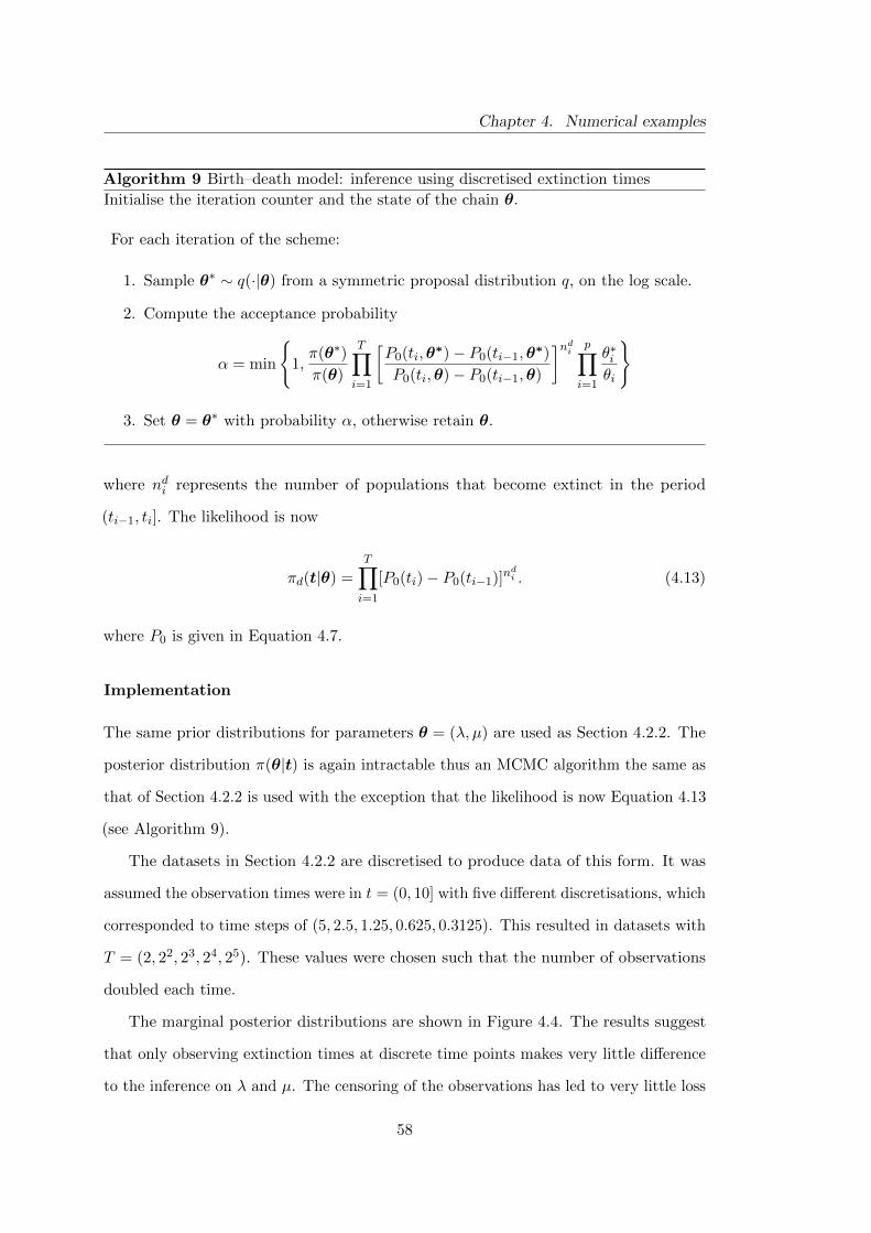
Chapter 4. Numerical examples
Algorithm 9 Birth–death model: inference using discretised extinction times
Initialise the iteration counter and the state of the chain θ.
For each iteration of the scheme:
1. Sample θ∗ ∼ q(·|θ) from a symmetric proposal distribution q, on the log scale.
2. Compute the acceptance probability
α = min
{1,π(θ∗)
π(θ)
T∏i=1
[P0(ti,θ
∗)− P0(ti−1,θ∗)
P0(ti,θ)− P0(ti−1,θ)
]ndi p∏i=1
θ∗iθi
}
3. Set θ = θ∗ with probability α, otherwise retain θ.
where ndi represents the number of populations that become extinct in the period
(ti−1, ti]. The likelihood is now
πd(t|θ) =T∏i=1
[P0(ti)− P0(ti−1)]ndi . (4.13)
where P0 is given in Equation 4.7.
Implementation
The same prior distributions for parameters θ = (λ, µ) are used as Section 4.2.2. The
posterior distribution π(θ|t) is again intractable thus an MCMC algorithm the same as
that of Section 4.2.2 is used with the exception that the likelihood is now Equation 4.13
(see Algorithm 9).
The datasets in Section 4.2.2 are discretised to produce data of this form. It was
assumed the observation times were in t = (0, 10] with five different discretisations, which
corresponded to time steps of (5, 2.5, 1.25, 0.625, 0.3125). This resulted in datasets with
T = (2, 22, 23, 24, 25). These values were chosen such that the number of observations
doubled each time.
The marginal posterior distributions are shown in Figure 4.4. The results suggest
that only observing extinction times at discrete time points makes very little difference
to the inference on λ and µ. The censoring of the observations has led to very little loss
58

Chapter 4. Numerical examples
of information about rate parameters of the process. Even with only two observations,
posterior distributions of the rate parameters are centered around the correct region
with variance only slightly larger than obtained when the extinction times are observed
exactly. The nature of the process means that the proportion of extinct populations is
monotonically increasing. As a result of this, observing the process at the beginning,
middle and end captures most of the vital kinetics.
4.2.4 Inference for noisy proportions of extinction
Suppose that the observed data are noisy proportions of extinction. This equates to
observing data as in Section 4.2.3 with measurement error. Denote the observed data
by xt and assume the following data model
yt = logitxt = logit pt(θ) + εt, t = 1, . . . , T (independent)
where pt(θ) denotes the probability of extinction at time t and the εt are independent
with εt ∼ N(0, σ2). It is of interest to learn about (θ, σ) and assuming a priori that θ
and σ are independent, the posterior distribution is
π(θ, σ|y) ∝ π(θ)π(σ)π(y|θ, σ).
4.2.5 Exact probability of extinction
For a given θ and x0, assuming that the probability of extinction, pt(θ) is known in
closed form, the likelihood is
π(y|θ, σ) =
T∏t=1
φ(yt|logit pt(θ), σ2
).
59

Chapter 4. Numerical examples
For the birth–death process, this probability is
pt(θ) =
(µ−µe(µ−λ)tλ−µe(µ−λ)t)
)x0, forλ 6= µ(
λt1+λt
)x0, forλ = µ.
(4.14)
4.2.6 Approximate probability of extinction
In the scenario where pt(θ) is not known exactly, a simulation based approach can be
used to estimate pt(θ). The method was described in Section 4.2.1 and can be used to
simulate the time evolution of a population for a particular choice of θ and x0. This can
be converted to a binary time series denoting the extinction status of the population at
discrete time points t = 1, . . . , T . Repeating this for n populations gives
npt,n(θ) ∼ Bin(n, pt(θ))
where pt,n(θ) is the observed proportion of extinction. pt,n(θ) is an approximation of
pt(θ) and as n→∞, the approximation approaches the true proportion.
4.2.7 Approaches to inference
Three different approaches to inference will be considered, a likelihood-free vanilla
MCMC scheme and two pseudo-marginal schemes. The first pseudo-marginal scheme
has a Monte Carlo estimate of the marginal likelihood and the second has a Sequential
Monte Carlo estimate. These methods will be known as pseudo-marginal 1 and pseudo-
marginal 2. The theory behind each of these methods was described in Chapter 3. The
vanilla and pseudo-marginal schemes were previously applied to the constant model.
The detailed algorithms are given for the birth–death model in Algorithms 10 and 11.
The third approach is to use a sequential Monte Carlo estimate of the marginal
likelihood rather than a Monte Carlo estimate. The scheme outlined in Algorithm 12
uses a particle filter (SIR filter, Algorithm 5) at each iteration to construct an estimate
of the marginal likelihood. This approach is discussed in detail in Section 3.4.4.
60

Chapter 4. Numerical examples
Algorithm 10 Birth–death model: inference using the vanilla scheme
Initialise the iteration counter and the state of the chain (θ, σ).
For each iteration of the scheme:
1. Sample (θ∗, σ∗) ∼ q(·|θ, σ) from a symmetric proposal distribution q, on the logscale.
2. Simulate the path pn(θ∗) = [p1,n(θ), p2,n(θ), . . . , pT,n(θ)]T for some choice of n.
3. Compute the acceptance probability
α = min
{1,π(θ∗)
π(θ)
π(σ∗)
π(σ)
π(y|θ∗, σ∗)π(y|θ, τ)
θ∗
θ
τ∗
τ
}.
4. Set (θ, σ) = (θ∗, σ∗) with probability α, otherwise retain (θ, σ).
When using the SIR filter, it is necessary to store the states of the system. Let z1:n1:t
denote the state of the system for n populations up to time t, where
z1:n1:t =
z11 . . . z21 . . . zn1...
......
z1i . . . z2i . . . zni...
......
z1t . . . z2t . . . znt
.
The pt,n(θ) is deterministically related to z1:n1:t via the function h, where z1:n1:t represents
n simulations of the process up to time t
pt,n(θ) = h(z(1:n)1:t
)=
1
n
n∑i=1
I(zit 6=0).
For the birth–death process there is only one state for each population, namely the level
of the population. The pt,n is calculated by counting up the number of populations in
which extinction has occurred at time t and dividing by n.
The estimate of the marginal likelihood is constructed by noting that an estimate of
61
Chapter 4. Numerical examples
Algorithm 11 Birth–death model: inference using pseudo-marginal scheme 1
Initialise the iteration counter and the state of the chain (θ, σ).
For each iteration of the scheme:
1. Sample (θ∗, σ∗) ∼ q(·|θ, σ) from a symmetric proposal distribution q, on the logscale.
2. For each particle 1, . . . , N , simulate a path p(1)n (θ∗), p(2)n (θ∗), . . . , p(N)n (θ∗) for
some choice of n.
3. Construct a Monte Carlo, unbiased estimate of π(y|θ∗, σ∗)
π(y|θ∗, σ∗) =1
N
N∑j=1
π(y|p(j)n (θ∗), σ∗)
where
π(y|p(j)n (θ∗), σ∗) =T∏i=1
π(yt|p(j)i,n(θ∗), σ∗)
4. Compute the acceptance probability
α = min
{1,π(θ∗)
π(θ)
π(σ∗)
π(σ)
π(y|θ∗, σ∗)π(y|θ, σ)
θ∗
θ
σ∗
σ
}.
5. Set (θ, σ) = (θ∗, σ∗) with probability α, otherwise retain (θ, σ).
π(yt+1|y1:t,θ∗, σ∗) is given by
1
N
N∑j=1
wt+1,j ,
where the wt+1,j are defined in Algorithm 12. An estimate of the marginal likelihood is
π(y|θ∗, σ∗) =
T−1∏t=0
1
N
N∑j=1
wt+1,j
.
62

Chapter 4. Numerical examples
Algorithm 12 Birth–death model: inference using pseudo-marginal scheme 2
Initialise the iteration counter and the state of the chain (θ, σ).
For each iteration of the scheme:
1. Sample (θ∗, σ∗) ∼ q(·|θ, σ) from a symmetric proposal distribution q, on the logscale.
2. For each time t = 1, 2, . . . , T :
For each particle j = 1, 2, . . . , N :
(i) Draw z(1:n)t+1,j ∼ π
(·∣∣∣∣z(1:n)t,j ,θ∗
). Run the Gillespie algorithm from t to t+ 1
for 1:n paths.
(ii) Construct weights
wt+1,j = π
(yt+1
∣∣∣∣ h(z(1:n)t+1,j
), σ∗).
(iii) Calculate normalised weights
wnt+1,j =wt+1,j∑Nj=1wt+1,j
.
3. Resample N times amongst z(1:n)t+1,1, z
(1:n)t+1,2, . . . , z
(1:n)t+1,N using normalised weights as
probabilities.
4. Calculate
π(y|θ∗, σ∗) =
T−1∏t=0
1
N
N∑j=1
wt+1,j
.5. Compute the acceptance probability
α = min
{1,π(θ∗)
π(θ
π(σ∗)
π(σ)
π(y|θ∗, σ∗)π(y|θ, σ)
θ∗
θ
σ∗
σ
}.
6. Set (θ, σ) = (θ∗, σ∗) with probability α, otherwise retain (θ, σ).
63
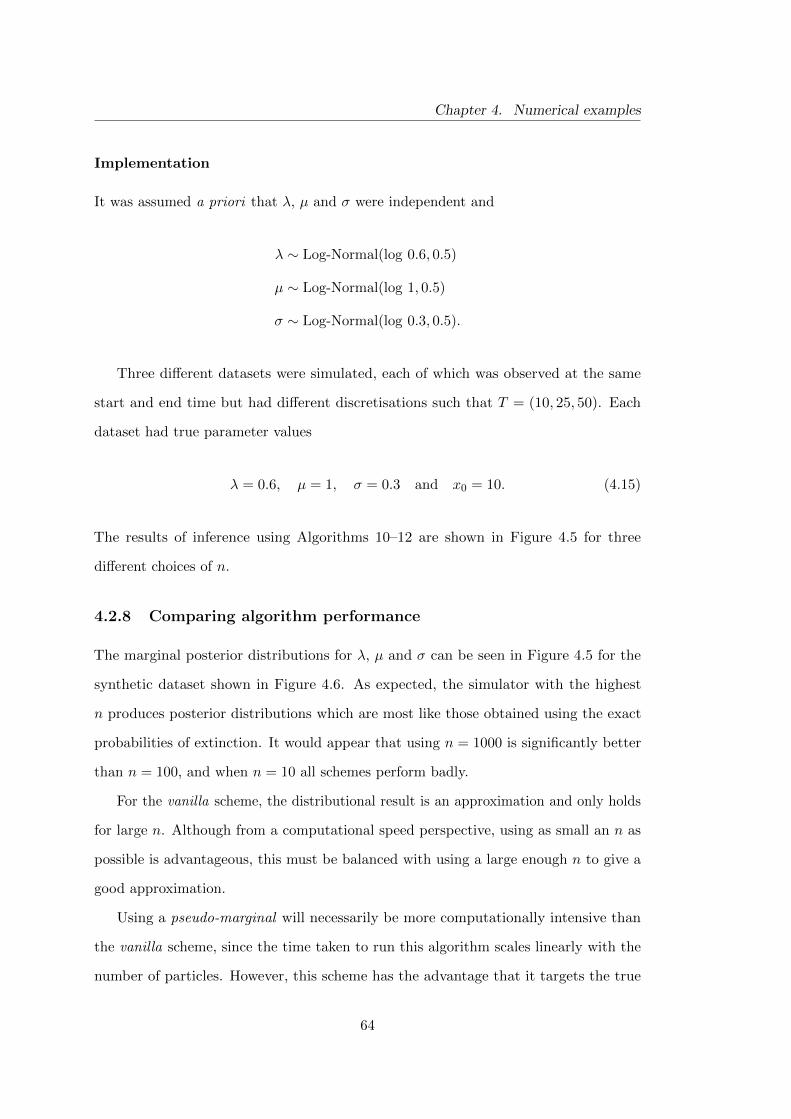
Chapter 4. Numerical examples
Implementation
It was assumed a priori that λ, µ and σ were independent and
λ ∼ Log-Normal(log 0.6, 0.5)
µ ∼ Log-Normal(log 1, 0.5)
σ ∼ Log-Normal(log 0.3, 0.5).
Three different datasets were simulated, each of which was observed at the same
start and end time but had different discretisations such that T = (10, 25, 50). Each
dataset had true parameter values
λ = 0.6, µ = 1, σ = 0.3 and x0 = 10. (4.15)
The results of inference using Algorithms 10–12 are shown in Figure 4.5 for three
different choices of n.
4.2.8 Comparing algorithm performance
The marginal posterior distributions for λ, µ and σ can be seen in Figure 4.5 for the
synthetic dataset shown in Figure 4.6. As expected, the simulator with the highest
n produces posterior distributions which are most like those obtained using the exact
probabilities of extinction. It would appear that using n = 1000 is significantly better
than n = 100, and when n = 10 all schemes perform badly.
For the vanilla scheme, the distributional result is an approximation and only holds
for large n. Although from a computational speed perspective, using as small an n as
possible is advantageous, this must be balanced with using a large enough n to give a
good approximation.
Using a pseudo-marginal will necessarily be more computationally intensive than
the vanilla scheme, since the time taken to run this algorithm scales linearly with the
number of particles. However, this scheme has the advantage that it targets the true
64

Chapter 4. Numerical examples
log λ log µ log σ
0
1
2
3
4
0
1
2
3
4
0
1
2
3
4
n=
10n
=100
n=
1000
−4 −3 −2 −1 0 1 −2 −1 0 1 2 −4 −3 −2 −1 0 1Parameter value
Den
sity
Vanilla MCMC Pseudo−marginal MCMC 1
Pseudo−marginal MCMC 2
Inference using exact probability of death
Figure 4.5: Marginal posterior distributions for log λ, log µ and log σ. Black vertical linesrepresent true values used to simulate data, grey lines represent the prior distribution.
65
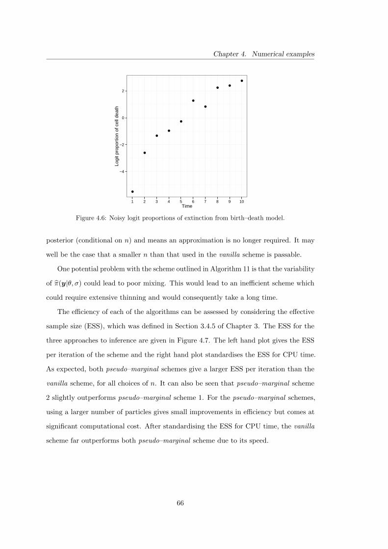
Chapter 4. Numerical examples
●
●
●
●
●
●
●
●●
●
−4
−2
0
2
1 2 3 4 5 6 7 8 9 10Time
Logi
t pro
port
ion
of c
ell d
eath
Figure 4.6: Noisy logit proportions of extinction from birth–death model.
posterior (conditional on n) and means an approximation is no longer required. It may
well be the case that a smaller n than that used in the vanilla scheme is passable.
One potential problem with the scheme outlined in Algorithm 11 is that the variability
of π(y|θ, σ) could lead to poor mixing. This would lead to an inefficient scheme which
could require extensive thinning and would consequently take a long time.
The efficiency of each of the algorithms can be assessed by considering the effective
sample size (ESS), which was defined in Section 3.4.5 of Chapter 3. The ESS for the
three approaches to inference are given in Figure 4.7. The left hand plot gives the ESS
per iteration of the scheme and the right hand plot standardises the ESS for CPU time.
As expected, both pseudo–marginal schemes give a larger ESS per iteration than the
vanilla scheme, for all choices of n. It can also be seen that pseudo–marginal scheme
2 slightly outperforms pseudo–marginal scheme 1. For the pseudo–marginal schemes,
using a larger number of particles gives small improvements in efficiency but comes at
significant computational cost. After standardising the ESS for CPU time, the vanilla
scheme far outperforms both pseudo–marginal scheme due to its speed.
66

Chapter 4. Numerical examples
ESS
●●●
●●●
●
●
●● ●●●
●
●●●
●
●●
●
0.02
0.04
0.06
0.08
0.02
0.04
0.06
0.08
0.02
0.04
0.06
0.08
n=
10n
=100
n=
1000
Pseudo marginal 1
Pseudo marginal 2
Vanilla
Method
ES
S
ESS standardised
●
●● ●●●
●
●●● ●●●
●
●●● ●●●
●
0.00
0.05
0.10
0.15
0.00
0.05
0.10
0.15
0.00
0.05
0.10
0.15
n=
10n
=100
n=
1000
Pseudo marginal 1
Pseudo marginal 2
Vanilla
Method
ES
S~
stan
dard
ised
Figure 4.7: Effective sample sizes (ESS). Left: ESS per iteration. Right: ESS standardised forCPU time. Colours represent different numbers of particles in the pseudo marginal schemes: 10particles (green), 50 particles (blue), 100 particles (purple).
67

Chapter 5
Gaussian process emulation
The aim of this thesis is to make inferences about parameters in the PolyQ model,
a large stochastic kinetic model. One crucial component of the problem is that the
experimental data are proportions of cell death, not observations on the underlying
chemical species. The inferential task is not straightforward since the data likelihood is
intractable.
Chapter 3 describes several simulation based, likelihood-free inference strategies
which can be used to make inference on the parameters of the PolyQ model. These
algorithms all require the use of simulation to estimate the proportion of cell death, for
a proposed set of parameters. This involves obtaining n forward simulations from the
stochastic model to construct an estimate of the proportion of cell death. This must be
done at each iteration of the scheme.
Chapter 4 implements the algorithms described in Chapter 3 on much smaller models.
In these cases, the computational time taken to run the algorithms is not large, taking in
the order of minutes or hours, rather than days or weeks. However, the computational
time does not scale well with the complexity of the model and, for the PolyQ model,
simulating from the model is slow, and the inference schemes described in Chapter 3
become infeasible.
Chapter 2 describes methods for approximating the stochastic kinetic model, such
as the τ -leap method and approximating the Markov jump process with the Chemical
68

Chapter 5. Gaussian process emulation
Langevin Equation. Unfortunately the increased speed gained from using these strategies
is not sufficient to facilitate inference from the PolyQ model, and hence, an alternative
approach must be sought.
The problem of having a model that is prohibitively slow to simulate from is a
generic one in the context of computer experiments, which are typically used to explore
real life phenomena. One area where computer models are used extensively is in the
climate sciences. For example, the HadOCC (Hadley Centre Ocean Carbon Cycle model)
model (Palmer and Totterdell, 2001; Hemmings et al., 2008) models the ocean carbon
cycle. When computer experiments are computationally expensive to run, a much faster
approximation is sought.
The use of Gaussian processes to create a statistical model of a computer model,
known as an emulator is described in detail by Sacks et al. (1989); Currin et al. (1991);
Kennedy and O’Hagan (2001); Santner et al. (2003); O’Hagan (2006). Note, in the
geostatistics literature, kriging is used as a synonym for emulation. The idea is to run
the expensive simulator at only a limited number of input values and to infer the output
at new input values. These input values along with the simulator output are known
as the training data. The emulator can be thought of as a fast surrogate for the true
simulator which makes probabilistic predictions of the simulator output.
A naive approach to prediction would be to fit a regression model to the known
simulator outputs, and use this to predict the output for unknown inputs. However,
this ignores the fact that the uncertainty in the the prediction depends on how close
the prediction inputs are to inputs in the training dataset. Emulators are typically
constructed to produce fully probabilistic predictions of what the simulator would
produce. However, emulators that are constructed under the Bayes linear framework
only predict the mean and variance (Craig and Goldstein, 2001; Goldstein and Rougier,
2006).
Emulators are most commonly fitted to deterministic processes, where running the
simulator at the same inputs will produce identical outputs. There has been recent
interest in building emulators for stochastic models (Bates and Kenett, 2006; Henderson
69
Chapter 5. Gaussian process emulation
et al., 2009; Kleijnen, 2009). Despite the PolyQ model being a stochastic kinetic model,
the proportion of cell death through time is a deterministic process. This is because
given a very large number of cells governed by the PolyQ model, the proportion of
cells which die at time t is fixed. In what follows, a deterministic emulator will be
constructed to emulate proportions of cell death.
5.1 Building an emulator
Emulators are built using a set of training data which is obtained by running the
simulator for a particular set of inputs. These training input values are denoted
Θ = [θ1, . . . ,θi, . . . ,θnd ]T
which results in output values
y = [y(θ1), . . . , y(θi), . . . , y(θnd)]T .
In the context of cell death models, the y(θi) represent the logit proportions of cell
death. The dimension of θi is (np × 1); hence, this leads to a nd–point np–dimensional
design. More information on how choose the training design are given in Section 5.1.4.
It is necessary to determine a mean function which is denoted m(·) and typically
depends on parameters β. This could be, for example, a least squares fit to some
suitable functions of θ. It is also necessary to specify a covariance function K(·, ·),
which describes the relationship between the simulator output for inputs which are some
distance apart. The covariance function typically depends on unknown hyperparameters.
The aim is to learn about the simulator output at new inputs
Θ∗ = [θ∗1, . . . ,θ∗i , . . . ,θ
∗nd∗
]T
not featured in the training dataset. The corresponding test outputs about which
70

Chapter 5. Gaussian process emulation
inference is required are
y∗ = [y(θ∗1), . . . , y(θ∗i ), . . . , y(θ∗n∗d)]T .
Assuming a Gaussian Process prior
y ∼ N (m(Θ),K(Θ,Θ))
and
y∗ ∼ N (m(Θ∗),K(Θ∗,Θ∗)),
the joint distribution of y and y∗ is
y
y∗
∼ N m(Θ)
m(Θ∗)
,
K(Θ,Θ) K(Θ,Θ∗)
K(Θ∗,Θ) K(Θ∗,Θ∗)
.
Conditioning on the training outputs, the posterior for the test outputs is
y∗|y ∼ N (m∗,K∗)
where
m∗ = m(Θ∗) +K(Θ∗,Θ)TK(Θ,Θ)−1(y −m(Θ))
and
K∗ = K(Θ∗,Θ∗)−K(Θ∗,Θ)TK(Θ,Θ)−1K(Θ,Θ∗).
Note in the above, the explicit dependence of the hyperparameters on the mean
function m( · |·) and covariance function K( · |·) is dropped.
71

Chapter 5. Gaussian process emulation
5.1.1 Choice of mean function
It is necessary to define a mean function m(·) for the inputs, which is a function of θ.
The mean function must be carefully specified to ensure an accurate emulator. The
most simple choice is a zero order (constant) mean function, such that the regression
surface is flat. This amounts to expressing no prior knowledge about the likely output
of the simulator for a particular choice of θ. This approach is often used in practice,
see Sacks et al. (1989) and Oakley and O’Hagan (2004).
Caution must be taken when using a constant mean function as can be seen in
Figure 5.1. In the fourth plot, the hyperparameters of the covariance function are chosen
(for illustration purposes) so that the correlation between the outputs, at inputs which
are a small distance apart, is low. It can be seen that the mean function attempts to
revert to the prior (zero in this case) the further away from a training point it is. This
undesired effect is seen more generally in emulators when there is large distance between
training inputs, thus highlighting the need for a sensible choice of mean function.
Another common choice of mean function is a linear combination of the inputs
m(θ) = β0 +
np∑k=1
βkθk.
Examples of the use of this mean function can be seen in Oakley and O’Hagan (2004);
Conti and O’Hagan (2010). Other authors use more complex mean functions, such
as Kaufman et al. (2011) who constructed a mean function using Legendre polynomials.
A fully Bayesian approach to estimating the parameters of the mean function would
obtain a posterior distribution for the parameters. The marginal posterior distribution
of these parameters is a multivariate t-distribution. In general the number of points in
the Latin hypercube design nd will be large and so posterior uncertainty about these
parameters will be low. Therefore, in this thesis (unless stated otherwise), this level
of uncertainty is ignored and these parameters are fixed at their maximum likelihood
(least squares) estimates. This provides a simpler approach to fitting emulators.
72
Chapter 5. Gaussian process emulation
5.1.2 Choice of covariance function
The covariance function describes assumptions about the unknown function; it specifies
the covariance between the simulator output for a pair of inputs θi and θj . It can be
thought of as being a similarity measure, since it is expected that when the simulator is
run at pairs of inputs which are close together, the output will be similar.
The covariance function must generate a covariance matrix which is symmetric,
invertible and non-negative definite. It is typically the case that the covariance function
is chosen to be stationary. The stationarity property says that the covariance depends
only on the distance between two inputs |θi − θj | rather than the actual values of θi
and θj . It may be unrealistic to assume from the outset that the output varies similarly
in all areas of input space. However, it is hoped that after fitting an appropriate mean
function to the data, any large scale variation would be removed and a stationary
covariance function is suitable for the residuals.
The most common choice of covariance function is the squared exponential covariance
function and it has the form
K(θi,θj |a, r) = a exp
{−
np∑k=1
(θik − θjk)2/r2k
}
= aR(θi,θj |r).
Chapter 4 of Rasmussen and Williams (2006) gives an overview of further choices of
covariance functions and their properties.
This function depends on hyperparameters, (a, r). The physical interpretation of
these parameters is not immediately obvious. The vector r are known as the length
scale parameters; rk can be thought of as being a measure of how correlated outputs
will be at inputs θi and θj which are a distance |θi − θj | apart. Since the dimension of
r is equal to the dimension of the input, this covariance function allows different inputs
to impact the response differently.
73

Chapter 5. Gaussian process emulation
a = 0.1r = 0.2
a = 5r = 0.2
a = 10r = 0.2
a = 1r = 0.08
●●
●
●
●
●
●
●
●●
●
●
●
●
●
●
●●
●
●
●
●
●
●
●●
●
●
●
●
●
●
●●
●
●
●
●
●
●
●●
●
●
●
●
●
●
●●
●
●
●
●
●
●
●●
●
●
●
●
●
●
●●
●
●
●
●
●
●
●●
●
●
●
●
●
●
●●
●
●
●
●
●
●
●●
●
●
●
●
●
●
●●
●
●
●
●
●
●
●●
●
●
●
●
●
●
●●
●
●
●
●
●
●
●●
●
●
●
●
●
●
−6
−3
0
3
6
−1.0 −0.5 0.0 −1.0 −0.5 0.0 −1.0 −0.5 0.0 −1.0 −0.5 0.0log λ
Logi
t pro
port
ion
of d
eath
Figure 5.1: Emulation for logit proportions of death from the birth–death model (for fixedµ = 0.6). Training data shown in red. Mean and 2 standard deviations from the fitted GaussianProcess emulator shown in black. Different panels represent different choices of hyperparameters.
5.1.3 1-D birth–death example
Figure 5.1 depicts several fitted Gaussian process emulators to data obtained from the
birth–death model. In this example, the output (y-axis) is the logit probability that a
population becomes extinct and the input (x-axis) is the birth rate λ. Here the input θ
is one dimensional since the death rate µ is fixed at 0.6.
The red points denote the training data used to fit the emulator, the black lines
represent the fitted mean function and ±2 standard deviations. The different panels
represent emulators fitted with different choices of hyperparameters.
In the first three panels, the r parameter is kept constant and the a parameter
increases. It can be seen that effect of increasing a is to increase the emulator variance,
giving larger prediction intervals. In the fourth panel, the r parameter is much lower
than the others. In practice, this has the effect of lowering the influence of nearby
training points when making predictions. It can be seen that between training points,
the emulator attempts to revert to the prior mean function (zero in this case).
5.1.4 Training data design
It is necessary to choose carefully the θi at which to run the simulator. A poor choice
can lead to parts of the design space not being well explored which in turn can lead to
an inaccurate emulator in certain parts of the input space. In general, it is hoped that
74

Chapter 5. Gaussian process emulation
0.0 0.2 0.4 0.6 0.8 1.00.0
0.2
0.4
0.6
0.8
1.0
θ1
θ 2
●
●
●
●
●
Figure 5.2: Latin hypercube design in 2–D with nd = 5.
points are well spread out over the design space; a design is sought that is space filling.
The use of Latin hypercube sampling (LHS) was proposed by McKay et al. (1979)
as a space filling design. The popularity of this design can in part be attributed to its
ease of use. It was shown by Stein (1987) that when LHS is compared to simple random
sampling, it produces a lower asymptotic variance for the mean of simulator output.
In the two dimensional case, the design is a Latin square constructed by splitting
the space into np rows and columns and placing exactly one point in each row and
column as shown in Figure 5.2. When the Latin hypercube is projected onto either
axis, the points provide good coverage in that dimension. This generalises to higher
dimensions, where projecting the points onto any subset of the inputs produces a well
covered design. Although this design promises a well covered design when projected
onto any subset of the inputs, this does not necessarily ensure the whole space is well
covered. In the most extreme case, for two dimensions, the points could lie precisely on
the diagonal and still produce a valid Latin square.
Morris and Mitchell (1995) proposed the maximin design. Conceptually, this works
by maximising the distance between points. This is done by producing a list of the
minimum distance between points for each design using the Euclidean distance d(θ,θ′).
The maximin design maximises the minimum distance d(θ,θ′). Figure 5.3 compares
the ordinary Latin hypercube design with the maximin design in 2D with nd = 20. It
75

Chapter 5. Gaussian process emulation
Latin Hypercube Maximin
●
●
●
●
●
●
●
●
●
●
●
●
●
●
●
●
●
●
●
●●
●
●
●
●
●
●
●
●
●
●
●
●
●
●●
●
●
●
●
0.0
0.2
0.4
0.6
0.8
1.0
0.0 0.2 0.4 0.6 0.8 1.0 0.0 0.2 0.4 0.6 0.8 1.0θ1
θ 2
Figure 5.3: Left: Latin hypercube design. Right: Maximin design. Both with nd = 20.
can be seen that maximin design appears to given slightly better coverage of the design
space. In the following chapters, the maximin design will be used throughout.
The choice of nd represents a trade off between accuracy and speed since the
construction of an emulator involves multiple inversions of an nd×nd covariance matrix.
This operation scales with O(n3d); thus keeping nd as low as possible is vital. Chapman
et al. (1994) suggest that nd should be at least 10np.
5.2 Estimating hyperparameters
The fitted emulator is conditional on hyperparameters (a, r) which are unknown and
can be estimated from the standardised training data z(Θ) = y(Θ) − m(Θ). The
likelihood of these training data is
π(z|a, r) = (2π)−nd/2|K(a, r)|−1/2 exp
(−1
2zTK(a, r)−1z
)= (2π)−nd/2a−nd/2|R(r)|−1/2 exp
(− 1
2azTR(r)−1z
),
where the dependence of θi and θj on K(·, ·) and R(·) has been dropped from the
notation. A fully Bayesian analysis would specify a prior distribution for (a, r) and
proceed by obtaining the posterior distribution π(a, r|z), which is typically intractable.
An MCMC scheme can be constructed to obtain realisations of the posterior and these
can be used to obtain estimates of the hyperparameters.
76
Chapter 5. Gaussian process emulation
Under the assumption that the prior distribution has independent components and
a ∼ InvGa(c0, d0), a closed form for the marginal likelihood can be determined
π(z|r) =
∫ ∞0
π(z|a, r)π(a) da
=
∫ ∞0
(2π)−nd/2a−nd/2|R(r)|−1/2 exp
{− 1
2azTR(r)−1z
}× dc00 a
−c0−1e−d0/a
Γ (c0)da
=(2π)−nd/2dc00
Γ (c0)|R(r)|−1/2
∫ ∞0
a−c0−nd/2−1 exp
{−1
a
[d0 +
zTR(r)−1z
2
]}da.
On noting that ∫ ∞0
a−c−1e−d/c da = Γ (c)d−c
it follows that
π(z|r) =(2π)−nd/2dc00
Γ (c0)|R(r)|−1/2 × Γ (c0 + nd/2)
[d0 + zTR(r)−1z/2
]−(c0+nd/2)∝ |R(r)|−1/2
[1 +
zTR(r)−1z
2d0
]−(c0+nd/2)
where the proportionality constant does not depend on r. Further
π(a|r, z) ∝ π(z|a, r)π(a)
∝ |K(a, r)|−1/2 exp
{−1
2zTK(a, r)−1z
}a−c0−1e−d0/a
∝ a−nd/2 exp
{− 1
2azTR(r)−1z
}a−c0−1e−d0/a
∝ a−(c0+nd/2)−1 exp
{−1
a
[d0 +
zTR(r)−1z
2
]}
and so
a|r, z ∼ InvGa(c0 + nd/2, d0 + zTR(r)−1z/2
).
Therefore, assuming a priori a ∼ InvGa(c0, d0) independently of r allows an MCMC
scheme to be constructed with state space r (rather than a and r) which should
77

Chapter 5. Gaussian process emulation
Algorithm 13 Estimating hyperparameters 1
For each iteration of the scheme:
1. Propose r∗ ∼ q(r∗|r), where q is a symmetric random walk on the log scale.
2. Compute the acceptance probability α = min {1, A} where
A =π(r∗)
π(r)
π(z|r∗)π(z|r)
q(r|r∗)q(r∗|r)
=π(r∗)
π(r)
π(z|r∗)π(z|r)
np∏i=1
r∗iri.
If it is assumed the ri are independent a priori then the expression for A simplifiesto
A =π(z|r∗)π(z|r)
np∏i=1
r∗i π(r∗i )
riπ(ri).
3. Accept and move the current state of the chain to r∗ with probability α.
4. Simulate a from
a|r∗, z ∼ InvGa(c0 + nd/2, d0 + zTR(r∗)−1z/2
).
.
have better convergence properties and be more efficient. This algorithm is given in
Algorithm 13.
If it is assumed a priori ri ∼ LN(ci, 1/di), the numerator (or denominator) in the
acceptance probability A is given by
log
{π(z|r)
np∏i=1
riπ(ri)
}= k − 1
2log |R(r)| −
(c0 +
nd2
)log
(1 +
zTR(r)−1z
2d0
)
− 1
2
np∑i=1
di (log ri − ci)2 .
In Chapter 6, emulators are built for logit proportions of extinction for populations
governed by a birth–death model. When it is not possible to obtain exact proportions of
extinction from the model, approximate proportions can be obtained using many runs
of the simulator. This scenario was considered in detail in Section 4.2.6 of Chapter 4.
The uncertainty induced by this approximation can be accounted for in the emulator
78
Chapter 5. Gaussian process emulation
by introducing a nugget term to the covariance function
Kt(θi,θj |a, r) = Kt(θi,θj |a, r) + f(θi)δij
where δij is the Kronecker delta function and further details on the choice of f(·) are
given in Chapter 6. This amounts to adding an extra term to the leading diagonal of
the covariance matrix.
This means that the covariance function cannot be written in the form a×R. In
this case, the scheme presented in Algorithm 13 can no longer be used, since a cannot
be marginalised over. In this scenario, it is necessary to construct an MCMC scheme
with state space (a, r), that is, use a joint update as shown in Algorithm 14.
If it assumed a prior ri ∼ LN(ci, 1/di) and a ∼ LN(c0, 1/d0), the numerator (or
denominator) in the acceptance probability A is given by
log
{π(z|a, r)aπ(a)
np∏i=1
riπ(ri)
}= k − 1
2log |K(a, r)| − 1
2zT K(a, r)−1z
− d02
(log a− c0)2 −1
2
np∑i=1
di (log ri − ci)2 .
Once samples from the posterior have been obtained using either Algorithm 13 or 14,
emulator construction could proceed using a plug-in approach. For example, (a, r) could
be estimated using their marginal posterior mean/mode. Alternatively, the posterior
uncertainty could be taken into account and averaged over in the fitted emulators. Both
of these approaches are compared in the numerical examples in Chapter 6. For the
model considered, it was found that averaging over the posterior uncertainty in the
hyperparameters makes negligible difference to the emulator predictions.
5.3 Other approaches to hyperparameter estimation
One of the main drawbacks of Algorithms 13 and 14 is that the evaluation of the
likelihood, at each iteration, involves calculating both the determinant and the inverse
79
Chapter 5. Gaussian process emulation
Algorithm 14 Estimating hyperparameters 2
For each iteration of the scheme:
1. Propose (a∗, r∗) ∼ q(a∗, r∗|a, r), where q is a symmetric random walk withindependent components on the log scale.
2. Compute the acceptance probability α = min {1, A} where
A =π(a∗)
π(a)
π(r∗)
π(r)
π(z|a∗, r∗)π(z|a, r)
q(a|a∗)q(a∗|a)
q(r|r∗)q(r∗|r)
=π(a∗)
π(a)
π(r∗)
π(r)
π(z|a∗, r∗)π(z|a, r)
a∗
a
np∏i=1
r∗iri,
If it is assumed the ri are independent a priori then the expression for A simplifiesto
A =π(a∗)
π(a)
π(z|a∗, r∗)π(z|a, r)
a∗
a
np∏i=1
r∗i π(r∗i )
riπ(ri).
3. Accept and move the current state of the chain to (a∗, r∗) with probability α.
of the covariance matrix K. Inverting a matrix of size nd × nd is an O(n3d) operation,
hence the algorithm will scale with O(n3d) . Since the PolyQ model is high–dimensional,
using a large nd will be crucial to cover the parameter space. Consequently, a more
computational efficient approach to estimating hyperparameters must be sought.
5.3.1 Sparse covariance approach
To achieve the required computational speed up, one approach is to take advantage of
the near sparsity of the covariance matrix and use sparse matrix algorithms (Pissanetzky,
1984; Barry and Kelley Pace, 1997). This approach has received attention in the literature
in the context of covariance tapering (Furrer et al., 2006; Kaufman et al., 2008), where
the covariance matrix is multiplied by another sparse matrix to impose sparsity. These
methods all assume the correlation function is isotropic i.e. r1 = r2 = . . . = rnp . This
assumption is too restrictive since it is expected that for the PolyQ model, inputs will
impact the response differently.
The approach of Kaufman et al. (2011) allows anisotropic compactly supported
80

Chapter 5. Gaussian process emulation
0.00
0.25
0.50
0.75
1.00
−1.0 −0.5 0.0 0.5 1.0θi − θj
R(θ
i, θ j
)
Bohman Squared exponential
Figure 5.4: Comparison of the Bohman function and squared exponential kernel.
covariance functions. The inputs θ are first scaled so that they are in [0, 1] and the
covariance function is approximated by a function such as the Bohman function
Rk(t; τk)ij =
(1− t/τk) cos(πt/τk) + sin(πt/τk)/π, t < τk
0, t ≥ τk
where t = |θik − θjk|. The parameter τk governs the correlation in the output for input
k. The Bohman function is shown in Figure 5.4 (red line) for k = 1 and τ1 = 0.5. It
can be seen that the function is zero when t ≥ 0.5. The blue line illustrates the squared
exponential kernel where the hyperparameters are chosen such that the two functions
exhibit very similar behaviour. This function asymptotes zero when t gets large, but
unlike the Bohman function has no absolute cutoff for t after which R is taken to be
zero. The advantage of using a covariance function such as the Bohman is that is it still
creates a valid covariance matrix while allowing sparsity to be imposed.
The level of sparsity to be imposed on the covariance matrix is specified by the user
and represents a trade off between computational efficiency and accuracy. For example,
81
Chapter 5. Gaussian process emulation
s = 0.99 implies 99% of the off-diagonal elements of
R(t; τ )ij =
nP∏k=1
Rk(t; τk)ij
will be zero and this feeds into the prior for τ . It is assumed a priori that τ is uniformly
distributed over the space, such that each of the k inputs impacts the response equally
1
np
np∑k=1
τk ≤ c
where c is chosen to satisfy c(2− c) = (1− s)1/np .
To construct the covariance matrix, pairs of input values θi and θj such that
|θik − θjk| < τk for all dimensions k are identified. These pairs only are used to compute
R(τ )ij =
np∏k=1
Rk(|θik − θjk|; τk).
The spam package (Furrer and Sain, 2010) in R uses computationally efficient sparse
matrix methods to store and manipulate sparse covariance matrices. The the Cholesky
decomposition of R(τ ) is computed and used to circumnavigate the need to compute
directly the inverse of the covariance matrix. An outline of the algorithm is given in
Algorithm 15.
5.4 Diagnostics
Following the construction of an emulator, it is crucial to assess how well it performs as
a surrogate for the simulator. Bastos and O’Hagan (2009) provide a detailed overview
of diagnostics for emulators.
One reason for an inaccurate emulator could be that the hyperparameters of the
covariance function (a and r) have been incorrectly estimated. Misspecification of a
affects the credible intervals for predictions from the emulator. An overestimation leads
to credible intervals which are too wide and an underestimation leads to credible intervals
82
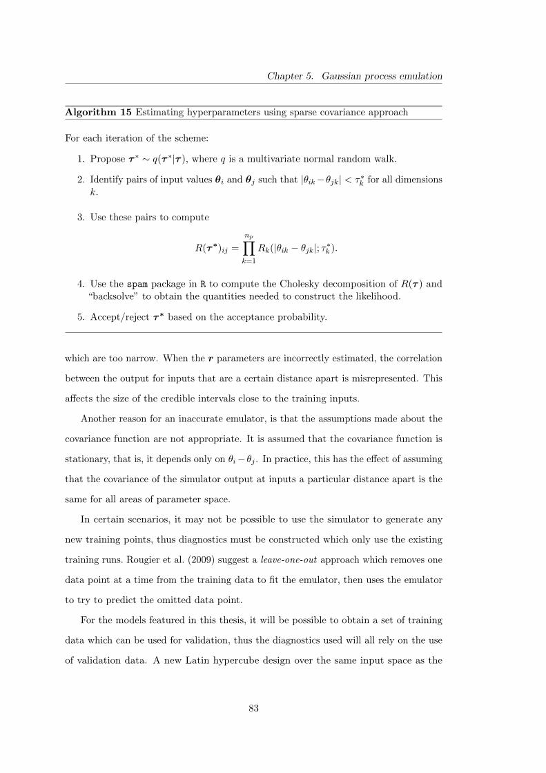
Chapter 5. Gaussian process emulation
Algorithm 15 Estimating hyperparameters using sparse covariance approach
For each iteration of the scheme:
1. Propose τ ∗ ∼ q(τ ∗|τ ), where q is a multivariate normal random walk.
2. Identify pairs of input values θi and θj such that |θik−θjk| < τ∗k for all dimensionsk.
3. Use these pairs to compute
R(τ ∗)ij =
np∏k=1
Rk(|θik − θjk|; τ∗k ).
4. Use the spam package in R to compute the Cholesky decomposition of R(τ ) and“backsolve” to obtain the quantities needed to construct the likelihood.
5. Accept/reject τ ∗ based on the acceptance probability.
which are too narrow. When the r parameters are incorrectly estimated, the correlation
between the output for inputs that are a certain distance apart is misrepresented. This
affects the size of the credible intervals close to the training inputs.
Another reason for an inaccurate emulator, is that the assumptions made about the
covariance function are not appropriate. It is assumed that the covariance function is
stationary, that is, it depends only on θi− θj . In practice, this has the effect of assuming
that the covariance of the simulator output at inputs a particular distance apart is the
same for all areas of parameter space.
In certain scenarios, it may not be possible to use the simulator to generate any
new training points, thus diagnostics must be constructed which only use the existing
training runs. Rougier et al. (2009) suggest a leave-one-out approach which removes one
data point at a time from the training data to fit the emulator, then uses the emulator
to try to predict the omitted data point.
For the models featured in this thesis, it will be possible to obtain a set of training
data which can be used for validation, thus the diagnostics used will all rely on the use
of validation data. A new Latin hypercube design over the same input space as the
83

Chapter 5. Gaussian process emulation
original is constructed which has n†d points
Θ† =
[θ†1, . . . ,θ
†i , . . . ,θ
†n†d
]
giving n†d outputs from the simulator
y† =
[y(θ†1), . . . , y(θ†i ), . . . y(θ†
n†d)
].
This new data (Θ†,y†) will be known as the validation training dataset.
5.4.1 Individual prediction errors
The individual prediction errors (IPE) are defined as
D(θ†i ) =y(θ†i )−m∗(θi
†)√K∗(θ†i , θ
†i )
for i = 1, . . . , n†d.
It is useful to use graphical summaries of the D(θ†i ) to assess emulator performance.
If the emulator is fitting correctly, the distribution of the D(θ†i ) should be standard
normal. It would be expected that approximately 95% of the IPE are within the interval
(−2, 2). Figure 5.5 (left-hand panel) gives an example of how the IPE would look if the
emulator was behaving as expected.
If the magnitude of the IPE is too large, this indicates that the emulator variance
has been underestimated. Conversely, too many very small values indicate that the
emulator variance is inflated.
Providing the emulator is fitting correctly, plots of the IPE would be expected to
have random scatter around zero with no patterns appearing. Plotting D(θ†i ) against θ†i
will indicate particular areas of parameter space in which the emulator is badly fitting.
Patterns in these plots could be a suggestion that the stationarity assumption of the
covariance function is not appropriate.
84
Chapter 5. Gaussian process emulation
5.4.2 Mahalanobis distance
The Mahalanobis distance is an extension to individual prediction errors which accounts
for the correlation in the outputs. It is defined as
MD2(Θ†) = {y(Θ†)−m∗(Θ†)}TK∗(Θ†,Θ†)−1{y(Θ†)−m∗(Θ†)}
and summarises the individual prediction errors in one single diagnostic. Conditional
on the training data and hyperparameters, it has distribution
MD2(Θ†) ∼ χ2n†d
since
y(θ†) ∼ Nn∗d
(m∗(θ†),K∗(θ†,θ†)
).
5.4.3 Probability integral transform
Gneiting et al. (2007) suggest using the Probability integral transform (PIT) to check
that the distributional assumptions of the emulator are reasonable. The PIT is defined
as
P (θ†i ) = Φ{D(θi†)} for i = 1, . . . , n†d.
If the distributional assumptions about the emulator are correct then D(θ†i ) should have
a standard normal distribution and P (θ†i ) should have a standard uniform distribution.
Plotting a histogram of P (θ†i ) should look flat if the Gaussian assumption of the emulator
is correct. Figure 5.5 (right-hand panel) illustrates how the PIT histogram should look
for a well behaved emulator. The PIT can be regarded as an alternative graphical
display of the IPE, allowing departures from the distributional assumptions of the
emulator to be viewed more easily.
85

Chapter 5. Gaussian process emulation
●
●
●
●
●
●
●
●
●
●
●
●
●
●●
●
●
●
●●
●●
●
●
●
●●●
●
●
●
●●
●
●
●
●
●
●
●●
●●●
●
●
●
●●
●
●
●
●
●
●
●
●●
●●
●
●●
●
●
●
●
●
●
●
●
●
●
●
●●
●
●
●
●
●
●
●
●
●
●
●
●
●●
●
●
●
●●
●●
●
●
●
−4
−2
0
2
4
0 25 50 75 100Index
IPE
0.0
0.5
1.0
0 1PIT
Den
sity
Figure 5.5: Example diagnostics with n†d = 50. Plot of the IPE (left) and PIT histogram (right).
86
Chapter 6
Parameter inference using
Gaussian process emulators
This chapter constructs Gaussian process emulators using the methodology outlined
in Chapter 5 for proportions of extinction from the birth–death model. The fit of the
emulators will be assessed using the diagnostics introduced in Chapter 5. Once the
fitted emulators have been constructed, they will be embedded into an inference scheme
and used in place of a simulator to make inferences about model parameters.
In Chapter 4, simulation–based inference schemes were successfully used to infer rate
parameters. These inference schemes all relied on the ability to quickly obtain forward
simulations from the model at each iteration. For the birth–death model, repeated
simulation from the model is quick, hence these simulation–based algorithms are feasible.
However, for larger models such as the PolyQ system, repeated simulation from the
model at each iteration of an inference scheme is too slow for practical purposes. This
motivates the need to find a fast approximation to the simulator and a Gaussian process
emulator provides this speed–up.
Since the birth–death model is quick to simulate from, the results of parameter
inference using the emulator can be compared to the results obtained in Chapter 4 using
the simulator.
87

Chapter 6. Parameter inference using Gaussian process emulators
6.1 Emulator construction
As in Chapter 4, noisy observations xt of proportions of extinction are observed discretely
in time; a plot of the observed data was given in Figure 4.6 of Chapter 4. The data are
assumed to have the following data model
yt(θ) ≡ logitxt(θ) = logit pt(θ) + σεt, t = 1, . . . , T
where the εt are independent and εt ∼ N(0, 1). For the birth–death model, the proportion
of extinction pt(θ) for different choices of θ = (λ, µ) is given by
pt(θ) =
(µ−µe(µ−λ)tλ−µe(µ−λ)t)
)x0, forλ 6= µ(
λt1+λt
)x0, forλ = µ
(6.1)
where x0 is the initial population level.
A Gaussian process emulator is required for output values yt(θ) = logit pt(θ). At
each time point t = 1, . . . , T , a Gaussian process emulator is fitted to output values
yt(θi) = logit pt(θi) for i = 1, . . . , nd
by evaluating Equation 6.1 at input values θi, i = 1, . . . , nd. These fitted emulators
have mean function
m∗t (Θ∗) = mt(Θ
∗) +Kt(Θ∗,Θ)TKt(Θ,Θ)−1(yt −mt(Θ)) (6.2)
and covariance function
K∗t (Θ∗,Θ∗) = Kt(Θ∗,Θ∗)−Kt(Θ
∗,Θ)TKt(Θ,Θ)−1Kt(Θ,Θ∗), (6.3)
these expression were derived in Section 5.1 of Chapter 5. Note that the explicit
dependence of the fitted covariance function on hyperparameters is omitted here for
88

Chapter 6. Parameter inference using Gaussian process emulators
notational simplicity. The hyperparameters a and r are estimated using the scheme
outlined in Algorithm 13 of Section 5.2. Further discussion regarding the estimation
and treatment of hyperparameters is given in Sections 6.1.5 and 6.2.2.
6.1.1 Emulating approximate proportions
For models that are more complex than the birth–death model, such analytic results
as Equation 6.1 are not available; consequently, this scenario must be explored. For
the birth–death model, the proportion of extinction can be approximated using n
runs of the simulator. This has been previously discussed in detail in Section 4.2.6 of
Chapter 4, where the approximate proportions are denoted pt,n. The empirical logit of
the approximate proportion is
elogit pt,n = log
(npt,n + 0.5
n− npt,n + 0.5
).
Gaussian process emulators can be constructed for output values
y(θ) = elogit pt,n(θ) for i = 1, . . . , nd
by running the simulator at input values θi, i = 1, . . . , nd. The distribution of elogit pt,n
is known for large n and this sampling error can be incorporated by including a nugget
term in the covariance function
Kt(θi,θj |a, r) = Kt(θi,θj |a, r) +δij
[n eexpitmt(θi){1− eexpitmt(θi)}]
where δij is the Kronecker delta function and eexpit is the inverse of the empirical logit,
i.e.
eexpitmt(θi) =emt(θi)(n+ 0.5)− 0.5
n[1 + emt(θi)].
In practice, the addition of the nugget term to the covariance function contributes only
to the leading diagonal elements of the covariance matrix. This causes the mean of the
89

Chapter 6. Parameter inference using Gaussian process emulators
fitted emulator to no longer go through all of the training points, and the emulator
variance is no longer zero at training points.
This effect can be seen for the one–dimensional birth–death example (with fixed
µ) given in Figure 6.1. The panels show emulators fitted to the empirical logit of
approximate proportions, simulated using n = 10, 102, 103, 104. The fitted mean function
no longer goes precisely through all of the points and the fitted variance is no longer zero
at training points. It can be seen that the nugget term has a much larger effect when n
is small. When n > 100, the effect of the nugget can barely be noticed. This behaviour
is desirable; when n is small, the approximation is much cruder than when n is large
and the emulator uncertainty should reflect this. Unless otherwise stated, approximate
proportions are constructed using n = 1000 runs of the simulator throughout the rest of
the thesis.
For emulation with approximate proportions, the construction proceeds as in the
previous section where K is replaced with K. The fitted mean and covariance are
m∗t (Θ∗) = mt(Θ
∗) + Kt(Θ∗,Θ)T Kt(Θ,Θ)−1(yt −mt(Θ)) (6.4)
and
K∗t (Θ∗,Θ∗) = Kt(Θ∗,Θ∗)− Kt(Θ
∗,Θ)T Kt(Θ,Θ)−1Kt(Θ,Θ∗). (6.5)
Since the covariance function K(·, ·) can no longer be written as a×R(·, ·), the scheme
for estimating hyperparameters introduced in Algorithm 13 of Section 5.2 may no longer
be used. However, the scheme presented in Algorithm 14 where a is not marginalised
over can be used.
Comment on emulator construction
The above approach fits Gaussian process emulators to output values yt(θi) at each
time point t = 1, . . . , T . This results in the construction of T emulators, each of which
90

Chapter 6. Parameter inference using Gaussian process emulators
n = 10 n = 100 n = 1000 n = 10000
●
●
●
●
●
●
●
●
●
●
● ●
● ●
●
●
●
●
●●
●
●
●
●
●●
●
●
●
●
●
●
−6
−3
0
3
6
−1.0 −0.5 0.0 −1.0 −0.5 0.0 −1.0 −0.5 0.0 −1.0 −0.5 0.0log λ
logi
t pro
port
ion
of d
eath
Figure 6.1: 1-D example of fitted emulator. Training data used to build emulator shown in redpoints. The mean and two standard deviations from the fitted emulator are shown in black. Thedifferent panels represent emulators built on approximate proportions where n = 10, 102, 103, 104
(where n is the number of forward simulations from the model used to construct proportions).
has input space with the same dimension as θ.
An alternative approach would have been to build a single emulator which has an
extra dimension for time t. The advantage of this approach is that it only requires
the construction of a single emulator; in this respect the implementation is simpler.
This was tried in practice; however, it was found that the number of design points nd
required was much larger since they had to cover the space of the extra input, t.
It has been decided that the first approach will be most suitable. Firstly, the times
at which experimental data are observed are known, there will be no need to make
predictions at new time points. Secondly, the construction of the emulator scales with
order O(n3d) since evaluating the likelihood for the hyperparameters involves inverting
the nd × nd covariance matrix. Having T smaller emulators will be computationally
beneficial and the construction of the emulators can also be parallelised.
6.1.2 Training data design
An appropriate area of parameter space must be selected over which to obtain the
training data. For the birth–death model, the aim is to make inferences on rate
parameters λ and µ. A sensible choice would be to use prior beliefs about λ and µ to
guide this choice. In Chapter 4, it was assumed a priori that λ and µ were independent
91

Chapter 6. Parameter inference using Gaussian process emulators
and
λ ∼ Log-Normal(log 0.6, 0.5)
µ ∼ Log-Normal(log 1, 0.5).
The Latin hypercube for the emulator will be constructed to cover the central 95%
of the prior distributions for log λ and log µ. If there is found to be much posterior
support in an area of parameter space not covered by the design space, then re-fitting
the emulators over a larger design space may be sensible. It must also be noted that
provided an appropriate prior mean function is specified, predictions for inputs outside
of the design space should still be sensible.
The Latin hypercube will be constructed for the log parameters since the inference
scheme uses a random walk over the log parameters. The range of the Latin hypercube
is
−1.9 < log λ < 0.88
−1.4 < logµ < 1.4.
The training data can be seen in Figure 6.2 for nd = 50, where the Latin hypercube
was constructed using the maximin design discussed in Chapter 5.
6.1.3 Choice of mean function
Before fitting the emulators, an appropriate prior mean function m(θ) must be chosen.
When the fitted emulator attempts to make predictions for inputs which are far away
from training inputs, the predicted mean reverts to the prior mean function. For this
reason, a careful choice of prior mean function is necessary. Further discussion on the
choice of prior mean function was given in Section 5.1.2 of Chapter 5.
Before deciding on a mean function, it is helpful to consider the shape of the function
to be emulated. Figure 6.3 illustrates the birth–death process. The left hand panel
92

Chapter 6. Parameter inference using Gaussian process emulators
●
●
●
●
●
●
●
●
●
●
●
●
●
●
●
●
●
●
●
●
●
●
●
●
●
●
●
●
●
●
●
●
●●
●
●
●
●
●
●
●
●
●
●
●
●
●
●
●
●
−1.5
−1.0
−0.5
0.0
0.5
1.0
1.5
−2 −1 0 1log λ
log
µ
−20−10010
Logit proportion of extinction
Figure 6.2: Birth–death model: training data used to build emulators shown in black dots; thebackground shows how the logit proportion of extinction varies with log λ and log µ .
log λ (µ = 0.6) log µ (λ = 1)
−20
−10
0
10
−2 −1 0 1 −1.5 −1.0 −0.5 0.0 0.5 1.0 1.5Parameter value
Logi
t pro
port
ion
of e
xtin
ctio
n
−1.5
−1.0
−0.5
0.0
0.5
1.0
1.5
−2 −1 0 1log λ
log
µ
−20−10010
Logit proportion of extinction
Figure 6.3: Birth–death model: logit proportions of extinction plotted against log λ for fixed µ(left), against log µ for fixed λ (middle), against log λ and log µ (right).
93
Chapter 6. Parameter inference using Gaussian process emulators
Number Mean Function
a β0b β0 + β1 log λ+ β2 logµc β0 + β1 log λ+ β2 logµ+ β3(log λ)2 + β4(logµ)2 + β5 log λ logµ
Table 6.1: Mean functions.
shows how the logit proportion of extinction changes with log λ (for fixed µ = 1) and
for logµ (for fixed λ = 0.6). The right hand panel shows how the logit proportion
of extinction changes for both log λ and logµ. Clearly it can be seen that the logit
proportion of extinction decreases with λ and increases with µ. This is expected, since
increasing the birth rate λ will cause the population level to increase, hence reducing
the likelihood of the population becoming extinct. The converse is true for an increase
in the death rate µ.
Table 6.1 presents three different choices of mean function. Mean function (a)
represents a constant mean function which expresses no prior beliefs about the simulator
output at different inputs. Mean function (b) includes linear terms in log λ and logµ
and mean function (c) includes higher order terms to reflect the non-linear behaviour.
When fitting the Gaussian process emulator the β parameters in the mean function are
fixed at the maximum likelihood (least squares) estimates.
6.1.4 Choice of covariance function
Since the birth–death process has two parameters, the squared exponential covariance
function takes the form
K(θi,θj |a, r) = a exp
{−(
(θi1 − θj1)2
r21+
(θi2 − θj2)2
r22
)}
and
K(λi, µi, λj , µj |a, r) = a exp
{−(
(log λi − log λj)2
r21+
(logµi − logµj)2
r22
)}.
94

Chapter 6. Parameter inference using Gaussian process emulators
There are three hyperparameters to be estimated a, r1 and r2. The parameter r1
relates to the effect the λ parameter has on the output and r2 relates to the effect the µ
parameter has on the output.
The use of this covariance function has the property that the mean of the fitted
emulator will go though all of the design points and the variance will be zero at these
points. This is appropriate behaviour for a deterministic simulator.
It was found in practice that this choice of covariance function presents computational
difficulties when attempting to compute the inverse of the covariance matrix. This is due
to the fact that the condition number (the ratio of the largest and smallest eigenvalues)
becomes too large. It is well known that covariance matrices of this form suffer from this
problem (Ababou et al., 1994; Neal, 1997). A common way to overcome this problem is
to add a jitter (or nugget) parameter to the covariance function, i.e.
K(θi,θj |a, r, g) = a
(exp
{−(
(θi1 − θj1)2
r21+
(θi2 − θj2)2
r22
)}+ gδij
)
where δij is the Kronecker delta function and g is the jitter parameter. In practice,
this has the effect of adding a small constant down the leading diagonal of the matrix.
This is very effective in reducing numerical instabilities. It has been suggested that the
jitter term should be as close to zero as is possible while still overcoming the numerical
instabilities (Ranjan et al., 2011).
In the context of the birth–death model, the addition of the jitter term was initially
sought purely for the purposes of preventing the covariance function becoming ill-
conditioned. Since g was thought to serve no real purpose, a small value of g was chosen
(approximately 10−6) and used for each emulator.
However, on further investigation it became clear that there are other advantageous
reasons for including the jitter term. Gramacy and Lee (2010) strongly claim that even for
deterministic simulators, omitting a jitter term is foolish. They present several reasons
why including a jitter term is a good idea. These arguments focus on the better statistical
properties which are achieved when a jitter term is included. In particular, Gramacy
95
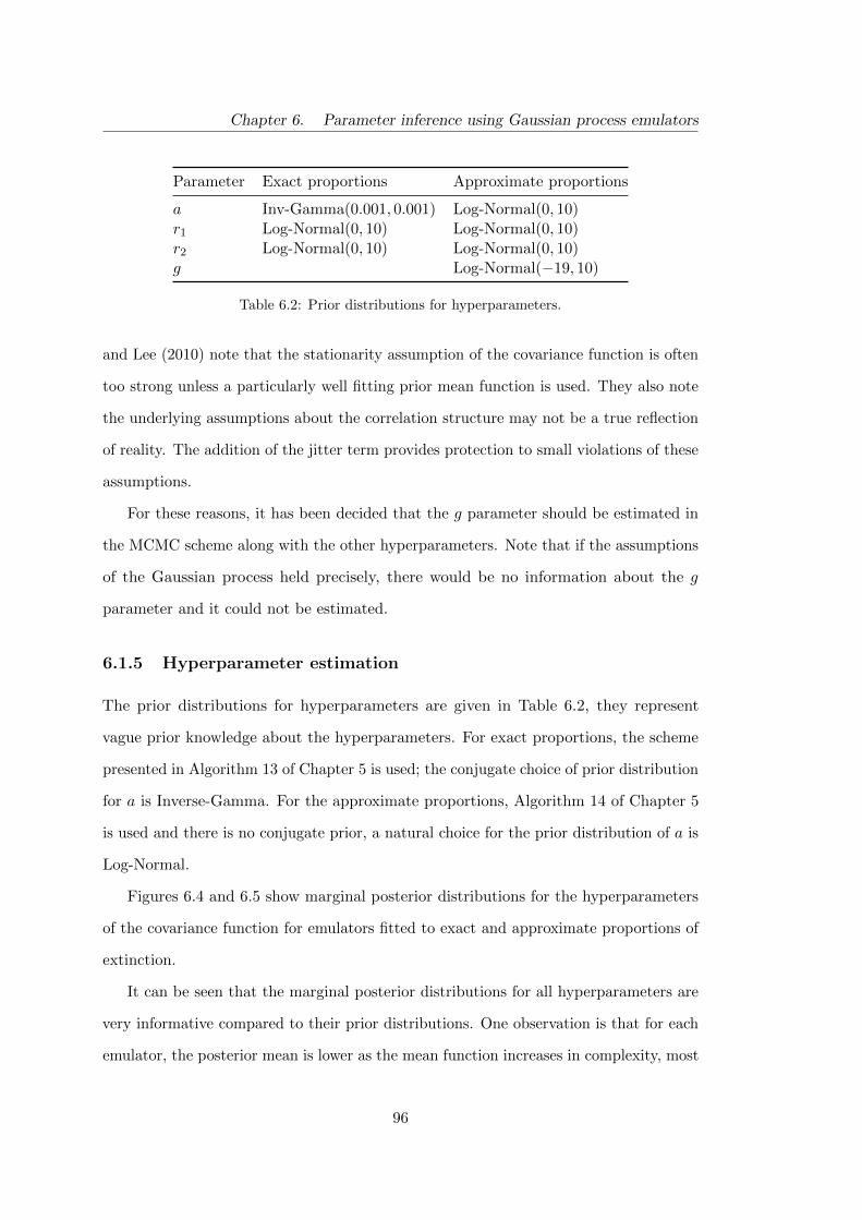
Chapter 6. Parameter inference using Gaussian process emulators
Parameter Exact proportions Approximate proportions
a Inv-Gamma(0.001, 0.001) Log-Normal(0, 10)r1 Log-Normal(0, 10) Log-Normal(0, 10)r2 Log-Normal(0, 10) Log-Normal(0, 10)g Log-Normal(−19, 10)
Table 6.2: Prior distributions for hyperparameters.
and Lee (2010) note that the stationarity assumption of the covariance function is often
too strong unless a particularly well fitting prior mean function is used. They also note
the underlying assumptions about the correlation structure may not be a true reflection
of reality. The addition of the jitter term provides protection to small violations of these
assumptions.
For these reasons, it has been decided that the g parameter should be estimated in
the MCMC scheme along with the other hyperparameters. Note that if the assumptions
of the Gaussian process held precisely, there would be no information about the g
parameter and it could not be estimated.
6.1.5 Hyperparameter estimation
The prior distributions for hyperparameters are given in Table 6.2, they represent
vague prior knowledge about the hyperparameters. For exact proportions, the scheme
presented in Algorithm 13 of Chapter 5 is used; the conjugate choice of prior distribution
for a is Inverse-Gamma. For the approximate proportions, Algorithm 14 of Chapter 5
is used and there is no conjugate prior, a natural choice for the prior distribution of a is
Log-Normal.
Figures 6.4 and 6.5 show marginal posterior distributions for the hyperparameters
of the covariance function for emulators fitted to exact and approximate proportions of
extinction.
It can be seen that the marginal posterior distributions for all hyperparameters are
very informative compared to their prior distributions. One observation is that for each
emulator, the posterior mean is lower as the mean function increases in complexity, most
96

Chapter 6. Parameter inference using Gaussian process emulators
notably for the a parameter. The a parameter can be thought of a general variance
term and represents the variability in the output. As the mean function becomes more
complex, more variability is removed from the residuals and it would be expected that
the a parameter would be lower.
Additionally, r1 and r2 are generally lower as the mean function becomes more
complex. This is also expected since larger values of ri imply the output is more
dependent on input i.
For the emulators fitted to exact proportions, there was the extra jitter parameter
g to estimate. This parameter describes the lack of fit of the model, for example, due
to violations of the assumptions of the Gaussian process emulators. It was seen that
for the most simple mean function, the posterior is most peaked, suggesting that there
is most information about g when a less complicated mean function is used. This is
as expected; it is more likely that the assumptions of the Gaussian process have been
violated if an inadequate mean function is used.
97

Chapter 6. Parameter inference using Gaussian process emulators
Time = 1 Time = 2 Time = 3 Time = 4 Time = 5 Time = 6 Time = 7 Time = 8 Time = 9 Time = 10
0.0
0.3
0.6
0.9
0.0
2.5
5.0
7.5
10.00.0
2.5
5.0
7.5
10.00.0
2.5
5.0
7.5
10.00.0
2.5
5.0
7.5
10.00.0
2.5
5.0
7.5
10.00.0
2.5
5.0
7.5
10.00.0
2.5
5.0
7.5
10.00.0
2.5
5.0
7.5
10.00.0
2.5
5.0
7.5
10.00.0
2.5
5.0
7.5
10.0
log a
Den
sity
Time = 1 Time = 2 Time = 3 Time = 4 Time = 5 Time = 6 Time = 7 Time = 8 Time = 9 Time = 10
0
2
4
6
0.0
0.5
1.0
1.5
0.0
0.5
1.0
1.5
0.0
0.5
1.0
1.5
0.0
0.5
1.0
1.5
0.0
0.5
1.0
1.5
0.0
0.5
1.0
1.5
0.0
0.5
1.0
1.5
0.0
0.5
1.0
1.5
0.0
0.5
1.0
1.5
0.0
0.5
1.0
1.5
log r1
Den
sity
Time = 1 Time = 2 Time = 3 Time = 4 Time = 5 Time = 6 Time = 7 Time = 8 Time = 9 Time = 10
0
2
4
6
8
−0.5
0.0
0.5
1.0
−0.5
0.0
0.5
1.0
−0.5
0.0
0.5
1.0
−0.5
0.0
0.5
1.0
−0.5
0.0
0.5
1.0
−0.5
0.0
0.5
1.0
−0.5
0.0
0.5
1.0
−0.5
0.0
0.5
1.0
−0.5
0.0
0.5
1.0
−0.5
0.0
0.5
1.0
log r2
Den
sity
Time = 1 Time = 2 Time = 3 Time = 4 Time = 5 Time = 6 Time = 7 Time = 8 Time = 9 Time = 10
0.0
0.2
0.4
0.6
−40
−30
−20
−10
−40
−30
−20
−10
−40
−30
−20
−10
−40
−30
−20
−10
−40
−30
−20
−10
−40
−30
−20
−10
−40
−30
−20
−10
−40
−30
−20
−10
−40
−30
−20
−10
−40
−30
−20
−10
log g
Den
sity
Figure 6.4: Marginal posterior distributions for hyperparameters for emulators fitted to exactproportions of extinction. Mean function (a) is given in red, mean function (b) green and meanfunction (c) in blue. Prior distributions are shown in black.
98
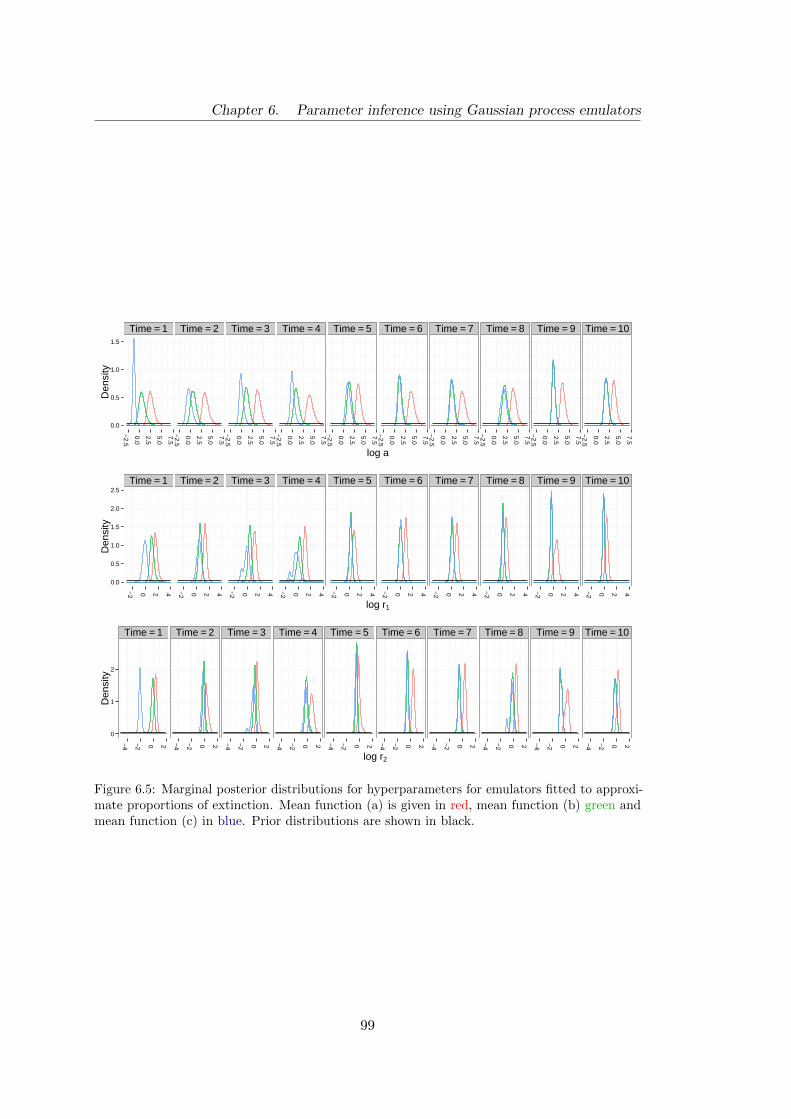
Chapter 6. Parameter inference using Gaussian process emulators
Time = 1 Time = 2 Time = 3 Time = 4 Time = 5 Time = 6 Time = 7 Time = 8 Time = 9 Time = 10
0.0
0.5
1.0
1.5
−2.5
0.0
2.5
5.0
7.5−
2.5
0.0
2.5
5.0
7.5−
2.5
0.0
2.5
5.0
7.5−
2.5
0.0
2.5
5.0
7.5−
2.5
0.0
2.5
5.0
7.5−
2.5
0.0
2.5
5.0
7.5−
2.5
0.0
2.5
5.0
7.5−
2.5
0.0
2.5
5.0
7.5−
2.5
0.0
2.5
5.0
7.5−
2.5
0.0
2.5
5.0
7.5
log a
Den
sity
Time = 1 Time = 2 Time = 3 Time = 4 Time = 5 Time = 6 Time = 7 Time = 8 Time = 9 Time = 10
0.0
0.5
1.0
1.5
2.0
2.5
−2 0 2 4 −2 0 2 4 −2 0 2 4 −2 0 2 4 −2 0 2 4 −2 0 2 4 −2 0 2 4 −2 0 2 4 −2 0 2 4 −2 0 2 4
log r1
Den
sity
Time = 1 Time = 2 Time = 3 Time = 4 Time = 5 Time = 6 Time = 7 Time = 8 Time = 9 Time = 10
0
1
2−
4
−2 0 2 −4
−2 0 2 −4
−2 0 2 −4
−2 0 2 −4
−2 0 2 −4
−2 0 2 −4
−2 0 2 −4
−2 0 2 −4
−2 0 2 −4
−2 0 2
log r2
Den
sity
Figure 6.5: Marginal posterior distributions for hyperparameters for emulators fitted to approxi-mate proportions of extinction. Mean function (a) is given in red, mean function (b) green andmean function (c) in blue. Prior distributions are shown in black.
99

Chapter 6. Parameter inference using Gaussian process emulators
6.1.6 Diagnostics
Diagnostics for the fitted emulators can be seen in Figures 6.6 (for exact proportions)
and 6.7 (for approximate proportions) for a validation dataset simulated consisting of
n†d = 25 points. The Latin hypercube over which the validation dataset was constructed
was over the same parameter range as the training data. The diagnostics used were
explained in detail in Section 5.4 of Chapter 5.
In each figure, the top plot shows the IPE (individual prediction errors). If the
emulators are fitting correctly, it would be hoped that most of the IPE values lie between
±2. It would also be hoped that the points would be randomly scattered around zero
with no obvious patterns.
The IPE (y-axis) are plotted against λ (x-axis) and coloured according to µ. This is
to check that the emulators are fitting well in all areas of parameter space. It can be
seen that there is no obvious pattern in the IPE for any of the choices of mean function.
The middle plot shows the PIT histograms for the fitted emulators. It would be
hoped that the PIT values have a standard uniform distribution. It can be seen that
there are deviations from the standard uniform distribution which suggests that the
tails of the emulators are slightly too heavy.
The bottom plot shows the Mahalanobis distance, which takes into account the
correlation in the residuals. For this diagnostic, there is only one value for each emulator
and making comparisons between the fit of different emulators is more convenient. It
can be seen that the Mahalanobis distances are all well below the upper 99% percentile
of χ225 distribution suggesting well fitting emulators. It is concluded that the fit of the
emulators is acceptable.
100

Chapter 6. Parameter inference using Gaussian process emulators
Time = 1 Time = 2 Time = 3 Time = 4 Time = 5 Time = 6 Time = 7 Time = 8 Time = 9 Time = 10
●● ●
●●
●●● ●●
●
●
●●
●
●
●
●●
●●
●
●
●
●
●
●
●
● ●
●
●●●
●●
●
●
●
●●
●●
●●
●
●● ●
●
●
●●● ●●
●
●
●
● ●
●
●
●● ●
●
●
●
●
●
●
●
●
●●
●●
●
●●●
●
●
●●
●
●● ●
●
●
●
●
●
●
●
●
●
●
●●
●
●
●
●
●
●
●●
●
●● ●
●
●
●
●
●
●
●●
●●
●●
●
●●
●
●
●
●●
●
●
●●
●
●
●
●
●
●
●
●
●
●
●●
●
●
●
●
●
●●
●
●
●●
●
●●
●
●
●
●
●
●
●
●●
●
●●●
●
●●
●
●
●
●
●
●●
●
●
●
●
●
●●
●●
●
●
●
●●
●●
●
●
●
●
●
●●
●●
●
●
●
●
●●
● ●
●
●
●●
●●
●
●
●
●
●
●●
●●
●
●
●
●
●●
●●
●
●●
●
●●
●
●
●
●
●
●●
●●
●
●
●
●●
●●
●
●
●
●●
●●
●
●●
●
●
●●●
●●
●
●
●
●●
●
●●
●●●
●●
●
●
●
●
●
●●
●●
●
●
●
●
●●
●
●●
●●●
●●
●
●
●
●
●
●●
●●
●
●
●
●●
●●
●●
●
●●●●
●
●● ●●
●●
●●
●
●
●
●
●
●●
●
●
●
●●
●
● ●● ●
●●
●
●●● ●
●
●
●
●
●
●
●●
●
●
●
●●
●
●●
● ●
●●
●
●●
●
●●
●
●
●
●
●
●●
●
●●
●
●
●
●●●
●
●●
● ●●
●●
●
●
●
●
●
●●●
●●
● ●●
●
● ●
●●
●● ● ●●
● ●●
●
●
●
●
●
●●
●
●
●●
●
●
●●
●●
●●● ●
●
●
●●
●
●
●
●
●
●●
●
●
●
●●
●
●●
● ●
●●
●●
●
● ●●●
●
●
●
●●
●●
●
● ●●
●
● ●
●●
●● ●
●
●
●●
●
●
●
●
●
●
●●
●
●
● ●
●
●
●●
●
●
●● ●
●
●
●
●●
●
●
●
●
●
●●
●
●
●●
●
●
●●
● ●
●●
●
●
●
● ●● ●●
●
●
●●
●●
●
●●
● ●
● ●●
●
●
●●
●
●
●●
● ●
●
●
●
●
●●
●
●
●●
●●
● ●
●
●
●● ●
●
●
●
●●
●
●
●
●
●
●●
●
●
● ●
●
●
●●
●●
●●●
●
●
● ●●
●●
●
●
●●
●●
●
● ●
● ●
● ●●
●
●
●
●
●
●
● ●
●
●●
●
●
●
●●
●
●
●●
● ●
● ●
●
●
●●
●
●
●
●
●
●●
●
●
●
●
●●
●
●
●●
●●
●●
●●
−5.0
−2.5
0.0
2.5
5.0
−5.0
−2.5
0.0
2.5
5.0
−5.0
−2.5
0.0
2.5
5.0
Mean F
unction (a)M
ean Function (b)
Mean F
unction (c)
−1 0 −1 0 −1 0 −1 0 −1 0 −1 0 −1 0 −1 0 −1 0 −1 0
λ
Indi
vidu
al P
redi
ctio
n E
rror
s
Time = 1 Time = 2 Time = 3 Time = 4 Time = 5 Time = 6 Time = 7 Time = 8 Time = 9 Time = 10
0.0
0.5
1.0
1.5
2.0
0.0
0.5
1.0
1.5
2.0
0.0
0.5
1.0
1.5
2.0
Mean F
unction (a)M
ean Function (b)
Mean F
unction (c)
0 1 0 1 0 1 0 1 0 1 0 1 0 1 0 1 0 1 0 1
Probability Integral Transform, Φ(IPE)
Den
sity
●
●
●
●
●
●
●
●● ●
●
●
●●
●
●
●
●●
●
●
●
●●
●
●
●
●● ●
Mean Function (a) Mean Function (b) Mean Function (c)
0
50
100
150
0
50
100
150
0
50
100
150
1 2 3 4 5 6 7 8 9 10 1 2 3 4 5 6 7 8 9 10 1 2 3 4 5 6 7 8 9 10
Time
Mah
alan
obis
Dis
tanc
e
Figure 6.6: Diagnostic for the birth–death model for emulators fitted to exact proportions ofextinction.
101

Chapter 6. Parameter inference using Gaussian process emulators
Time = 1 Time = 2 Time = 3 Time = 4 Time = 5 Time = 6 Time = 7 Time = 8 Time = 9 Time = 10
●
●
●
●●
●
● ●
●
●●
●
●●
●●
● ●●●●
●●
●
●
●
●
●
●●
●
●●
●
●
●
●
● ●
●
●
●●●●
●●
●
●
●
●
●
● ●●●
●●●
●
●
●●
●
●
●
●●
●●
●●
● ●●
●●●
●
●
●● ●
●
●
●
●●
●
●
●
●
●
●
●●
●●
●●
●
●●
● ●
●●
●●●
●
●●
●
●
●
●●
●
● ●
●
●●●
●
●●
● ●
●●
●●
●
●
●
●
●
●
●●
●
●
●●
●
●
●●
●
●
●
●●
●● ●●
●● ●
●
● ●
●
●
●●
●
● ●
●
●●
●
●
●
● ●●
●
●●
●●
●
●●
●
●
●●
●
●
● ●●
●●
●
●●
● ●●
●
●●
●
●●
●●
●
●
●
●
●● ●●
● ●
●
●●
●
●
●
●●
●●
●●
●
●
●●
●
●
●
●
●
●●
●
●
●
●●●
● ●●●
●●●●
●
●
●●
●
●
●
●●
● ●●
●
●
●●●
●●
●●
●
●
●
● ●
●
●
●
●
●
●
●●
●●
●
●
●
●●●
●●●
●
●●
●
● ●●
●
●●
●
●
●●
● ●●
●●
●●
●● ●●●
●●●
● ●
●
●
●
●
●
●
●●
●●
● ●●
●●
●● ●●●
●●
●● ●●
●
●●
●
●
●●
●
●
●●●
●●
●
●●●●●
●●
●
●●
●
●
●
●
●
●●
●
●● ●
●
●●● ● ●
●
● ●●●
●
●
● ● ●
●
●
●
●
●
●
●
●●
●
●●● ● ●
●
● ●●
●
●
●
● ●●
●
●
●
●
●
●
●
●●
●
●
●
● ●
●
●
●●
●
●
●
●●●
●
●
●
●
●●
● ●●
●
●
●
●
●
●
●●● ●
●
●●
●● ●●
●
●
●
●●
●
●
●
●●
●
●
●
●
●●●
●●
●●
●●●
●●
●
●
●●
●
●
●
●●
●
●
●
● ●
●
● ●●
●
● ●●
●●
●●
●
●●● ●● ●
●
●
●
●
●●
●● ●
●●●
●● ● ●
●●
●
●● ● ●
●
●
●
●
●
●●
●
●●
●●
●
● ●● ● ●
●●
●
●● ●●
●●
●
●●
●
●
●●
●●
●●●
●●
●
●●
●●
●
●●
●
●●
●
●●● ●
●●● ●●
●
●
●●●
●
●
●
●
●
● ●
●
●
●●
●●● ● ●●● ●
●●
●
●●●
●●
●
●
●
● ●
●
●
●●
●●
●●
●
●
●●
●
●●
●●
●
● ●
●
●●
●
●●
●
●
●
●●
●●
●
●
● ●
●●● ●
●
●
●●
●
●●
●
● ●
●
●
●
●●
●●
●
●
● ●
●●● ●
●
●
●●
●
●●
●
● ●
●
●
●
−5.0
−2.5
0.0
2.5
5.0
−5.0
−2.5
0.0
2.5
5.0
−5.0
−2.5
0.0
2.5
5.0
Mean F
unction (a)M
ean Function (b)
Mean F
unction (c)
−1 0 1 −1 0 1 −1 0 1 −1 0 1 −1 0 1 −1 0 1 −1 0 1 −1 0 1 −1 0 1 −1 0 1
λ
Indi
vidu
al P
redi
ctio
n E
rror
s
Time = 1 Time = 2 Time = 3 Time = 4 Time = 5 Time = 6 Time = 7 Time = 8 Time = 9 Time = 10
0.0
0.5
1.0
1.5
2.0
0.0
0.5
1.0
1.5
2.0
0.0
0.5
1.0
1.5
2.0
Mean F
unction (a)M
ean Function (b)
Mean F
unction (c)
0 1 0 1 0 1 0 1 0 1 0 1 0 1 0 1 0 1 0 1
Probability Integral Transform, Φ(IPE)
Den
sity
●●
●
●
● ●
●●
● ●
●
● ●●
● ●
●
●
●●
●
●
●
●
● ●
●
●
●●
Mean Function (a) Mean Function (b) Mean Function (c)
0
50
100
150
0
50
100
150
0
50
100
150
1 2 3 4 5 6 7 8 9 10 1 2 3 4 5 6 7 8 9 10 1 2 3 4 5 6 7 8 9 10
Time
Mah
alan
obis
Dis
tanc
e
Figure 6.7: Diagnostic for the birth–death model for emulators fitted to approximate proportionsof extinction (with n = 1000).
102
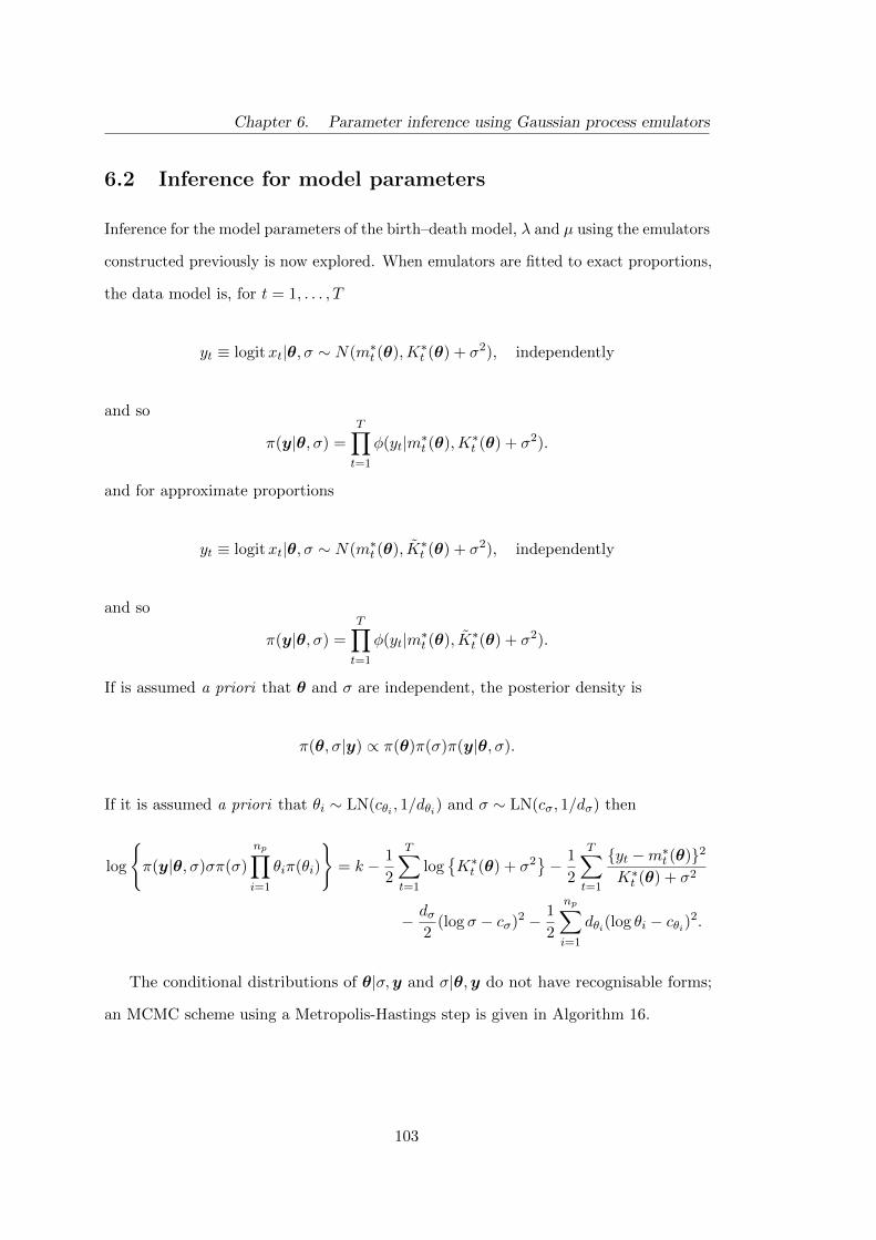
Chapter 6. Parameter inference using Gaussian process emulators
6.2 Inference for model parameters
Inference for the model parameters of the birth–death model, λ and µ using the emulators
constructed previously is now explored. When emulators are fitted to exact proportions,
the data model is, for t = 1, . . . , T
yt ≡ logitxt|θ, σ ∼ N(m∗t (θ),K∗t (θ) + σ2), independently
and so
π(y|θ, σ) =
T∏t=1
φ(yt|m∗t (θ),K∗t (θ) + σ2).
and for approximate proportions
yt ≡ logitxt|θ, σ ∼ N(m∗t (θ), K∗t (θ) + σ2), independently
and so
π(y|θ, σ) =
T∏t=1
φ(yt|m∗t (θ), K∗t (θ) + σ2).
If is assumed a priori that θ and σ are independent, the posterior density is
π(θ, σ|y) ∝ π(θ)π(σ)π(y|θ, σ).
If it is assumed a priori that θi ∼ LN(cθi , 1/dθi) and σ ∼ LN(cσ, 1/dσ) then
log
{π(y|θ, σ)σπ(σ)
np∏i=1
θiπ(θi)
}= k − 1
2
T∑t=1
log{K∗t (θ) + σ2
}− 1
2
T∑t=1
{yt −m∗t (θ)}2
K∗t (θ) + σ2
− dσ2
(log σ − cσ)2 − 1
2
np∑i=1
dθi(log θi − cθi)2.
The conditional distributions of θ|σ,y and σ|θ,y do not have recognisable forms;
an MCMC scheme using a Metropolis-Hastings step is given in Algorithm 16.
103

Chapter 6. Parameter inference using Gaussian process emulators
Algorithm 16 MCMC scheme for model parameters using emulators
For each iteration of the scheme:
1. Sample (θ∗, σ∗)T from a symmetric proposal distribution q, on the log scale.
2. Compute the acceptance probability
α = min
{1,π(θ∗)π(σ∗)
π(θ)π(σ)
π(y|θ∗, σ∗)π(y|θ, σ)
σ∗
σ
p∏i=1
θ∗iθi
}.
3. Set (θ, σ) = (θ∗, σ∗) with probability α, otherwise retain (θ, σ). else keep (θ, σ)T .
6.2.1 Results of inference using emulators
Results of inference on model parameters using emulators are given in Figure 6.8 (using
the same experimental data from Chapter 4), where the top panel relates to inference
using emulators with exact proportions of extinction, and the bottom panel relates to
inference with emulators using approximate proportions (with n = 1000). In Chapter 4,
these marginal posterior distributions were obtained using a simulator rather than an
emulator, the posterior distributions resulting from these schemes will be referred to
as exact or vanilla. It is advantageous that these gold standard posterior distributions
exist, since they provide a reference point for comparing emulator performance.
Firstly, considering the results for the exact proportions (top panel), it can be seen
that for all choices of mean function, comparing the marginal posterior distributions to
the exact posterior (red line), the difference is indistinguishable. This suggests that the
emulators are acting as an excellent surrogate to the simulator and are fairly insensitive
to the choice of mean function.
Secondly, considering the results for the approximate proportions (bottom panel), it
can be seen that, for all choices of mean function, the posterior distributions are very
close to those obtained when using the simulator.
104

Chapter 6. Parameter inference using Gaussian process emulators
log λ log µ log σ
0
1
2
3
4
0
1
2
3
4
Exact proportions
Approxim
ate proportions
−2 −1 0 1 −2 −1 0 1 −2.0 −1.5 −1.0 −0.5 0.0 0.5
Parameter Value
Den
sity
Simulator Emulator with mean function (a)
Emulator with mean function (b)
Emulator with mean function (c)
Figure 6.8: Results of inference on the birth–death model. Top panel: using emulators fitted toexact proportions of extinction. Bottom panel: using emulators fitted to approximate proportionsof extinction.
105
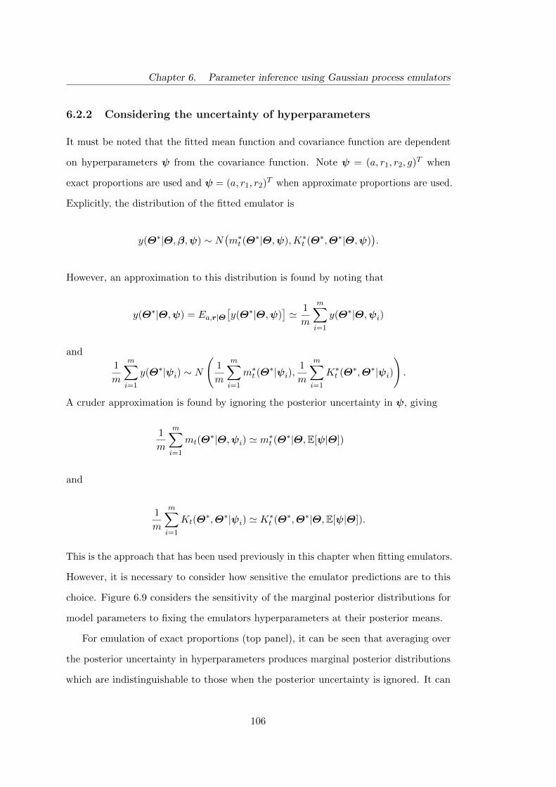
Chapter 6. Parameter inference using Gaussian process emulators
6.2.2 Considering the uncertainty of hyperparameters
It must be noted that the fitted mean function and covariance function are dependent
on hyperparameters ψ from the covariance function. Note ψ = (a, r1, r2, g)T when
exact proportions are used and ψ = (a, r1, r2)T when approximate proportions are used.
Explicitly, the distribution of the fitted emulator is
y(Θ∗|Θ,β,ψ) ∼ N(m∗t (Θ
∗|Θ,ψ),K∗t (Θ∗,Θ∗|Θ,ψ)).
However, an approximation to this distribution is found by noting that
y(Θ∗|Θ,ψ) = Ea,r|Θ[y(Θ∗|Θ,ψ)
]' 1
m
m∑i=1
y(Θ∗|Θ,ψi)
and
1
m
m∑i=1
y(Θ∗|ψi) ∼ N
(1
m
m∑i=1
m∗t (Θ∗|ψi),
1
m
m∑i=1
K∗t (Θ∗,Θ∗|ψi)
).
A cruder approximation is found by ignoring the posterior uncertainty in ψ, giving
1
m
m∑i=1
mt(Θ∗|Θ,ψi) ' m∗t (Θ∗|Θ,E[ψ|Θ])
and
1
m
m∑i=1
Kt(Θ∗,Θ∗|ψi) ' K∗t (Θ∗,Θ∗|Θ,E[ψ|Θ]).
This is the approach that has been used previously in this chapter when fitting emulators.
However, it is necessary to consider how sensitive the emulator predictions are to this
choice. Figure 6.9 considers the sensitivity of the marginal posterior distributions for
model parameters to fixing the emulators hyperparameters at their posterior means.
For emulation of exact proportions (top panel), it can be seen that averaging over
the posterior uncertainty in hyperparameters produces marginal posterior distributions
which are indistinguishable to those when the posterior uncertainty is ignored. It can
106

Chapter 6. Parameter inference using Gaussian process emulators
log λ log µ log σ
0
1
2
3
4
0
1
2
3
4
Exact proportions
Approxim
ate proportions
−2 −1 0 1 −2 −1 0 1 −2.0 −1.5 −1.0 −0.5 0.0 0.5
Parameter Value
Den
sity
Emulator with hyperparameters fixed at upper 97.5% of posterior
Emulator with hyperparameters fixed at lower 2.5% of posterior
Emulator averaging over hyperameter uncertainty
Figure 6.9: Results of inference on the birth–death model, considering the sensitivity to theposterior uncertainty in hyperparameters. Top panel: using emulators fitted to exact proportionsof extinction. Bottom panel: using emulators fitted to approximate proportions of extinction
107
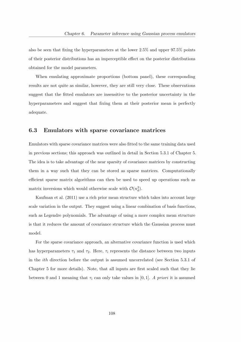
Chapter 6. Parameter inference using Gaussian process emulators
also be seen that fixing the hyperparameters at the lower 2.5% and upper 97.5% points
of their posterior distributions has an imperceptible effect on the posterior distributions
obtained for the model parameters.
When emulating approximate proportions (bottom panel), these corresponding
results are not quite as similar, however, they are still very close. These observations
suggest that the fitted emulators are insensitive to the posterior uncertainty in the
hyperparameters and suggest that fixing them at their posterior mean is perfectly
adequate.
6.3 Emulators with sparse covariance matrices
Emulators with sparse covariance matrices were also fitted to the same training data used
in previous sections; this approach was outlined in detail in Section 5.3.1 of Chapter 5.
The idea is to take advantage of the near sparsity of covariance matrices by constructing
them in a way such that they can be stored as sparse matrices. Computationally
efficient sparse matrix algorithms can then be used to speed up operations such as
matrix inversions which would otherwise scale with O(n3d).
Kaufman et al. (2011) use a rich prior mean structure which takes into account large
scale variation in the output. They suggest using a linear combination of basis functions,
such as Legendre polynomials. The advantage of using a more complex mean structure
is that it reduces the amount of covariance structure which the Gaussian process must
model.
For the sparse covariance approach, an alternative covariance function is used which
has hyperparameters τ1 and τ2. Here, τi represents the distance between two inputs
in the ith direction before the output is assumed uncorrelated (see Section 5.3.1 of
Chapter 5 for more details). Note, that all inputs are first scaled such that they lie
between 0 and 1 meaning that τi can only take values in [0, 1]. A priori it is assumed
108

Chapter 6. Parameter inference using Gaussian process emulators
that τ is uniformly distributed over the space
1
np
np∑k=1
τk ≤ c
where c is chosen to satisfy c(2− c) = (1− s)1/np .
The marginal posterior distributions for log τ1 and log τ2 can be seen in Figure 6.10
for different levels of sparsity. As the sparsity level increases, τ1 and τ2 get closer to zero.
This is to be expected as the greater the level of sparsity imposed on the matrix, the
smaller distance apart inputs can be before their outputs are considered uncorrelated.
Diagnostics for these emulators can be seen in Figures 6.11 (exact proportions)
and 6.12 (approximate proportions). Using the criteria discussed previously, it can be
seen that plots of the IPE show no unsually large values, however, the PIT histograms
confirm that there appear to be departures from normality in the IPE. However, it
must be noted that the sparse covariance approach represents an approximation with
considerable speed up, and it would be expected that these emulators do not fit as well
as those built under the original scheme.
The results of inference on model parameters using emulators can be seen in Fig-
ure 6.13. They are compared with the marginal posterior distributions obtained in
Chapter 4 using the simulator.
It can be seen that for exact proportions (top panel), emulators with sparse covariance
matrices provide posterior distributions for model parameters which are very similar to
those obtained using the simulator. However, it must be noted that as the sparsity level
increases, the posterior distributions start to look more different to results obtained
using the simulator.
For approximate proportions (bottom panel), λ and µ are well recovered. However,
the emulator has failed to capture the measurement error structure and the σ parameter
is not well recovered. This suggests that the emulator variance is inaccurate.
109
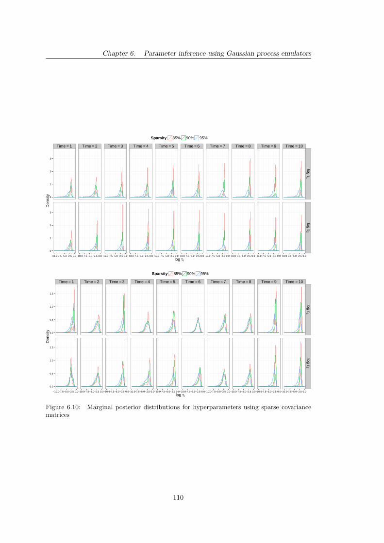
Chapter 6. Parameter inference using Gaussian process emulators
Time = 1 Time = 2 Time = 3 Time = 4 Time = 5 Time = 6 Time = 7 Time = 8 Time = 9 Time = 10
0
1
2
3
0
1
2
3
log τ1
log τ2
−10.0−7.5−5.0−2.5 0.0−10.0−7.5−5.0−2.5 0.0−10.0−7.5−5.0−2.5 0.0−10.0−7.5−5.0−2.5 0.0−10.0−7.5−5.0−2.5 0.0−10.0−7.5−5.0−2.5 0.0−10.0−7.5−5.0−2.5 0.0−10.0−7.5−5.0−2.5 0.0−10.0−7.5−5.0−2.5 0.0−10.0−7.5−5.0−2.5 0.0
log τi
Den
sity
Sparsity 85% 90% 95%
Time = 1 Time = 2 Time = 3 Time = 4 Time = 5 Time = 6 Time = 7 Time = 8 Time = 9 Time = 10
0.0
0.5
1.0
1.5
0.0
0.5
1.0
1.5
log τ1
log τ2
−10.0−7.5−5.0−2.5 0.0−10.0−7.5−5.0−2.5 0.0−10.0−7.5−5.0−2.5 0.0−10.0−7.5−5.0−2.5 0.0−10.0−7.5−5.0−2.5 0.0−10.0−7.5−5.0−2.5 0.0−10.0−7.5−5.0−2.5 0.0−10.0−7.5−5.0−2.5 0.0−10.0−7.5−5.0−2.5 0.0−10.0−7.5−5.0−2.5 0.0
log τi
Den
sity
Sparsity 85% 90% 95%
Figure 6.10: Marginal posterior distributions for hyperparameters using sparse covariancematrices
110

Chapter 6. Parameter inference using Gaussian process emulators
Time = 1Time = 10Time = 2 Time = 3 Time = 4 Time = 5 Time = 6 Time = 7 Time = 8 Time = 9
●●●
●
●
●●
●
●
●●
●
● ●●●
●
● ●
● ●● ●
● ●
●●● ●
●
●●
●
●●
●
●
● ●●●
●
● ●
● ●● ●●●
●●
●●
●
●●
●
●
●
●
●
● ●●●
●
● ●
●●
●●
● ●
●●
● ●●● ●●
●●●
●
●●●
●●
●●
● ●●●
●
●
●● ● ●●●●●
●●●
●
●●
●●
●●●
●●●
●
●
●
●●●
●●
● ●●
●●
●
●
●●
●
●●● ●●
●● ●
●
●
●
●● ●
●
●●●
●●
●
●
●●
●●
●
● ●● ●●
●●
●
●
●● ●
●
●●●
●●
●
●
●●●
●
●
● ●● ●●
●●
●
●
●●
●
●●
●●
●●
●
●●
●●
●
●
●●●
●
●
●
●
●
●
●● ●●
● ●●
●
● ●●●
●●
●
●
● ●● ●● ●●
●
●
●● ●
●● ●●
●●
●●●
●●
●
●
● ●● ●●
●●
●
●
●
●●●●
●●
●●
●●●
●●
●
●
● ●● ●●
●
●
●
●
●● ●
●● ●●
●
●
● ●●
●●●
●
● ●● ●●
●●
●
●
●● ●●● ●●
●●
● ●●
●●●
●
●●● ●
●
●
●
●
●
●
●
●●● ●
●
●●
● ●●
●●
●
●
● ●● ●●
●
●
●
●● ● ●
●● ●●
●
●●
●●
●●●
●
●●
● ●●
●●
●
●
●● ●●● ●●
●
●
●●
●●●
●
●
●●● ●●
●
●
●
●
●
●
●●● ●
●
●●●
●
●●●
●
●
● ●●●
●
●
●
●
●●
● ●●● ●●
●
●●
●
●●●
●●
●●●
●●
●
●
●
●
●●
●●● ●●
●
●●
●
●●
●
●
●
●●●
●●
●
●
●
●
●
●
●●● ●
●
●●●
●
●●●
●
●
● ●●●
●
●
●
●
●● ● ●●● ●●
●●
●
●
●
●●●
●●
●● ●
● ●
●
●
●
●● ●●● ●●
●●
●
●
●●●
●●
●●
● ●● ●
●
●
●
●
●
●●
● ●●
●●
●
●
●●●
●
●● ●●
●●●
●
●
●● ● ●●● ●●
●●
●
●
●●●
● ●●
●● ●● ●
●
●
●● ●
●●● ●●
●●
●
●
●●●
● ●●
●●
●● ●
●
●
●●
●
●●
● ●●
●●
●
●
●●
●
●●
● ●●
●●●
●
●
●●● ●●● ●
●
●●●
●
●●●
● ●●●
● ●●●
●
●
●● ● ●●● ●●
●●●
●
●●●
● ●●●
●●● ●
●
●
●●
●
●●
● ●●
●●●
●
●●
●
● ●● ●●
●● ●
●
●
−5.0
−2.5
0.0
2.5
5.0
−5.0
−2.5
0.0
2.5
5.0
−5.0
−2.5
0.0
2.5
5.0
85% sparse
90% sparse
95% sparse
−1 0 −1 0 −1 0 −1 0 −1 0 −1 0 −1 0 −1 0 −1 0 −1 0
λ
Indi
vidu
al P
redi
ctio
n E
rror
s
Time = 1 Time = 10 Time = 2 Time = 3 Time = 4 Time = 5 Time = 6 Time = 7 Time = 8 Time = 9
0
1
2
3
0
1
2
3
0
1
2
3
85% sparse
90% sparse
95% sparse
0 1 0 1 0 1 0 1 0 1 0 1 0 1 0 1 0 1 0 1
Probability Integral Transform, Φ(IPE)
Den
sity
Figure 6.11: Diagnostics for emulators with sparse covariance matrices fitted to exact proportions.
111

Chapter 6. Parameter inference using Gaussian process emulators
Time = 1 Time = 10 Time = 2 Time = 3 Time = 4 Time = 5 Time = 6 Time = 7 Time = 8 Time = 9
●●
●
●
●
● ●● ●●
●●
●
●●
●
● ●●
●●
●●
●
●
●●●
●
●
● ●●
●
●
●●
●
●●
●
● ●●●●
● ●
●
●
●●
●
●
●
●●
●
●●
●●
●●
●
●
● ● ●
●●
● ●
●
●
●
●
●
●
●● ●●
●●
●●
●
●
●
●●
●●●
●● ● ●●
●
●
●●
●● ●
●●
●
●●
●●
●
●
●●
●●●
● ● ●
●
●
●
●●●● ●●
●
● ●
●
●
●
●
●
●
●●●●
●
● ●
●
●
●
●
●
●●
●
●●
● ●●
●
●
●
●
●
●
●●●
●
●●
●
●
●
●
●
●●
●
●●●
●
●
●
●●
●
●
●
●
●
●
●
●●●
●
●
●
●
●
●
●●
●
●●
●
●
●
●
●
●
●
●
●
●●
●●
●●
●
●●●
●
●
●● ●
●●
●●
●
●● ●
●
●
● ●●
●
●●
●
●●
●●
●
● ●
●●
●
●
●
●
● ●
●
●
●● ●●
●
●●
●●
●
●
●●
●●
●
●●
●
● ●
●
●
●
●●
●
●
●
●
●
●
●
●
●
●●
●●
●
●●●
●
●●
●
●●●
●●
●●
●
●●
●
●
●
●●●
●
●
●●
●
●
●
●
●
●
●
●●●
●●
●
●●
●
●
●
●● ●
●
●
●●
●
●
●
●●
●●
●●●
●
●
●●●
● ●●
●
●
●●
●●
●
●
●●
●
●
●● ●
●
●
●
●
●
●●
●●●
●
●
●●
●
●●
●
●
●
●
●●● ● ●●
●
●
●
●●
●
●
●
●
●
●●
●
●
●
●
●
●
●
●
●●●
●
●
●
●●●●●
●●
●
● ●
● ● ●● ●●
●
●
●
●● ●
●●
●
●
●●
●●
●●
●
●
●● ●
●
●
●●
●
●
●
●●●
●
●
●
●●
●●
●
●●
●
●
●●
●●
●●
●
●
●
●
●● ● ●●
●
●
●
●
●
●
●
●
●
●
●●
●
●
●
●
● ●
●
●●
●● ●●
●
●
●
●
●
●
●
●
●
●
●●
●
●
●
●
● ●
●
●
●●
● ●
●
●
●
●
●
●
●
●
●
●
●
●●
●
●
●
●
●●
●
●
●●● ●
●
●
●
●
●●● ●● ●
●
●●
●●
●
●
●
●●●
●●● ●
●
●
●
●
●
●
● ●●●
●
●
●
●●
●
●
●
● ●
●
●●● ●
●
●
●
●
●
●
●
●
●
●
●●● ●
●
●
●
●
● ●●
●● ●●
●
●
●
●●
●
●
●●
●●
●
●
●
●
●
●
● ●●●
●● ●
●●
●
●
●●
●
●
●●
●●
●
●
●
●
●
●
●●
●●●
● ●
●●
●
●
●●
●
●
●
●●
●
●
●
●
●
●
●
●●
●●
●●
●
●●
−5.0
−2.5
0.0
2.5
5.0
−5.0
−2.5
0.0
2.5
5.0
−5.0
−2.5
0.0
2.5
5.0
85% sparse
90% sparse
95% sparse
λ
Indi
vidu
al P
redi
ctio
n E
rror
s
Time = 1 Time = 10 Time = 2 Time = 3 Time = 4 Time = 5 Time = 6 Time = 7 Time = 8 Time = 9
0
1
2
0
1
2
0
1
2
85% sparse
90% sparse
95% sparse
0 1 0 1 0 1 0 1 0 1 0 1 0 1 0 1 0 1 0 1Proability Integral Transform, Φ(IPE)
Den
sity
Figure 6.12: Diagnostics for emulators with sparse covariance matrices fitted to approximateproportions.
112
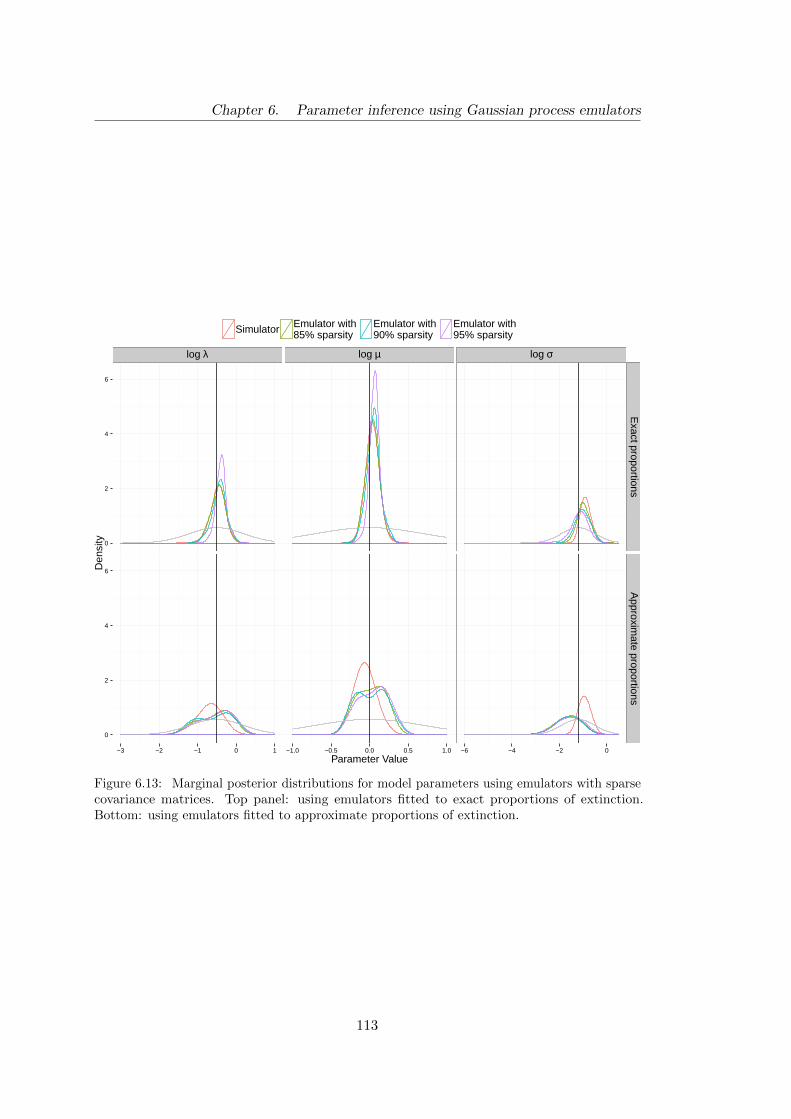
Chapter 6. Parameter inference using Gaussian process emulators
log λ log µ log σ
0
2
4
6
0
2
4
6
Exact proportions
Approxim
ate proportions
−3 −2 −1 0 1 −1.0 −0.5 0.0 0.5 1.0 −6 −4 −2 0
Parameter Value
Den
sity
Simulator Emulator with 85% sparsity
Emulator with 90% sparsity
Emulator with 95% sparsity
Figure 6.13: Marginal posterior distributions for model parameters using emulators with sparsecovariance matrices. Top panel: using emulators fitted to exact proportions of extinction.Bottom: using emulators fitted to approximate proportions of extinction.
113
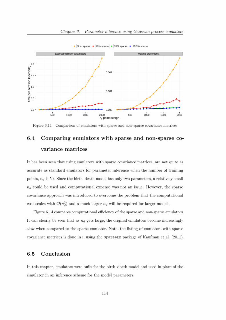
Chapter 6. Parameter inference using Gaussian process emulators
● ● ● ● ● ● ● ● ● ● ● ● ● ● ● ● ●●
● ●
● ● ● ● ● ● ● ● ● ● ● ● ● ● ● ● ● ● ● ●● ● ● ● ● ● ● ● ● ● ● ● ● ● ● ● ● ● ● ●● ● ● ●●
●●
●
●
●
●
●
●
●
●
●
●
●
●
●
● ● ● ● ● ● ● ● ● ● ●● ●
● ●● ●
●
●
●
● ● ● ● ● ● ● ● ● ● ● ● ● ● ● ● ● ● ● ●
● ● ● ● ● ● ● ● ● ● ● ● ● ● ● ● ● ● ● ●
● ● ● ● ●●
●●
●
●
●
●
●
●
●
●
●
●
●
●
Estimating hyperparameters Making predictions
0.0
0.5
1.0
1.5
2.0
0.000
0.001
0.002
500 1000 1500 2000 500 1000 1500 2000nd point design
time
per
itera
tion
(sec
onds
)
● ● ● ●Non−sparse 90% sparse 99% sparse 99.9% sparse
Figure 6.14: Comparison of emulators with sparse and non–sparse covariance matrices
6.4 Comparing emulators with sparse and non-sparse co-
variance matrices
It has been seen that using emulators with sparse covariance matrices, are not quite as
accurate as standard emulators for parameter inference when the number of training
points, nd is 50. Since the birth–death model has only two parameters, a relatively small
nd could be used and computational expense was not an issue. However, the sparse
covariance approach was introduced to overcome the problem that the computational
cost scales with O(n3d) and a much larger nd will be required for larger models.
Figure 6.14 compares computational efficiency of the sparse and non-sparse emulators.
It can clearly be seen that as nd gets large, the original emulators become increasingly
slow when compared to the sparse emulator. Note, the fitting of emulators with sparse
covariance matrices is done in R using the SparseEm package of Kaufman et al. (2011).
6.5 Conclusion
In this chapter, emulators were built for the birth–death model and used in place of the
simulator in an inference scheme for the model parameters.
114

Chapter 6. Parameter inference using Gaussian process emulators
In the first scenario, the training data were built on the exact proportions of
extinction since an analytic expression exists for this quantity. For emulators built under
this framework, it was found that a jitter parameter must be added to the covariance
function to ensure numerical stability. As discussed, the addition of this jitter term
has other desirable properties. It is confirmed by the emulator diagnostics that the
emulators are fitting acceptably.
When attempting to infer model parameters using emulators built on exact propor-
tions, it was found that using training data with nd = 50 gave inferences which were
indistinguishable from the true posterior. These posterior distributions appear to be
insensitive to the mean function. The posterior distributions also seem insensitive to
ignoring the posterior uncertainty in the hyperparameters.
It was found that using emulators with sparse covariance matrices fitted to exact
proportions provided inferences which were very similar to that of the inferences obtained
using the simulator. The much improved computational scaling of the sparse emulators
was clearly demonstrated.
In the second scenario, emulators were built for approximate proportions of extinction
simulated using n = 1000 runs of the simulator. In this case, a nugget term was added
to the covariance function to deal with the extra uncertainty induced. It was found that
even in this scenario, emulators performed as a very good surrogate for the simulator,
although not quite as good as when exact proportions were used.
The emulators with sparse covariance matrices did not perform as well when used
on approximate proportions. The fitted emulator mean is very good when compared to
the actual mean, although the emulator variance is inaccurate. Although initially, it
may seem that this approach will not be appropriate for approximate proportions, the
ease of use and speed of implementation make this approach ideal as a first attempt at
a larger problem.
115

Chapter 7
Mitochondrial DNA model
This chapter considers parameter inference, using Gaussian process emulators, for a
medium sized model of mitochondrial DNA (mtDNA). This model was first introduced
in Chapter 2 and will be studied in further detail in this chapter.
Inference has been attempted previously for this model. Henderson et al. (2009)
consider inference, when the experimental data are noisy measurements on one of the
underlying chemical species in the model. In a further paper, Henderson et al. (2010)
use an additional dataset containing counts of surviving neurons to make inferences
about model parameters.
In this chapter, interest lies in performing inference using only the data on proportions
of surviving neurons. For the purposes of this analysis, the binomial error on the
proportions is ignored. Firstly, inference will be attempted on simulated data, where
the true parameter values are known. This will give an idea of how well the method
performs. Secondly, inference will be attempted on the experimental data. It is hoped
that using only the data on proportions will be informative about model parameters,
and that these inferences are consistent with Henderson et al. (2009, 2010).
116

Chapter 7. Mitochondrial DNA model
7.1 A stochastic model
Sufferers of Parkinson’s disease exhibit symptoms which are related to the area of the
brain which controls motor function. It is also known that neuron loss in the substantia
nigra region of the human brain, located just above the spinal cord, is associated with
these symptoms.
The model aims to describe the process of neuron loss in the substantia nigra region.
Neuron loss is thought to be related to mtDNA deletions. Deletion mutations in the
mtDNA of the substantia nigra region are known to occur with ageing in healthy adults,
although higher levels have been observed in patients with Parkinson’s disease. It is of
scientific interest to gain a better understanding of how mtDNA deletions affect neuron
loss.
The focus of Henderson et al. (2009) was to use experimental data to perform
inference for the parameters of the mtDNA model. The motivation behind the analysis
in this chapter is to see what information is lost on model parameters by using only
proportions. The benefit of having posterior estimates of parameters is that they can
be used in a computer model which allows virtual experiments to be carried out. These
experiments could be used to determine interventions which can stop or reverse neuron
decline for suffers of Parkinson’s disease.
Model details
A brief introduction was given to the mtDNA model in Chapter 2. The model, for
a single neuron, involves two chemical species X = (X1, X2)′, where X1 represents
mtDNA with no deletions (healthy mtDNA) and X2 represents mtDNA with deletions
(unhealthy mtDNA). At any time, the number of copies of X1 and X2 is given by x1
and x2.
There are five possible reactions in the system which are given in Table 7.1. The
first reaction describes the process of mutation, whereby healthy mtDNA become
unhealthy mtDNA. The second and fourth reactions describe the process of synthesis
117

Chapter 7. Mitochondrial DNA model
Label Reaction Hazard Description
R1 X1 → X2 h1(x, θ1) = θ1x1 Mutation
R2 X1 → 2X1 h2(x, θ3) = 1000θ3x1x1+x2
Synthesis
R3 X1 → ∅ h3(x, θ3) = θ3x1 Degradation
R4 X2 → 2X2 h4(x, θ3) = 1000θ3x2x1+x2
Mutant Synthesis
R5 X2 → ∅ h5(x, θ3) = θ3x2 Mutant Degradation
Table 7.1: Reactions and their hazards for the mtDNA model.
(reproduction); this can happen in both the healthy and unhealthy mtDNA. The third
and fifth reactions describe degradation (death), which can also happen in both the
healthy and unhealthy mtDNA.
The original model given in Table 2.3 of Chapter 2 contains parameters θ =
(θ1, θ2, θ3, θ4, θ5)T . Henderson et al. (2009) make the assumption that healthy and
unhealthy mtDNA synthesise and degrade at the same rate, reducing the parameter
space to θ = (θ1, θ3)T , and giving the reaction hazards in Table 7.1. The rate laws for
reactions R2 and R4 are constructed to ensure that the total number of mtDNA in the
cell x1 + x2 remains approximately constant (at 1000) throughout the lifetime of the
cell.
The model contains a mechanism for cell death (neuron death). This is modelled by a
deterministic process in which the proportion of unhealthy mtDNA reaches some critical
threshold and the cell dies. The proportion of unhealthy mtDNA is p = x2/(x1 + x2)
and the model imposes cell death when p ≥ τ , for some threshold parameter τ ∈ (0, 1].
Deletion accumulation data
The experimental data used for inference in Henderson et al. (2009) were taken from
post–mortems of 15 individuals who ranged from 19 − 91 in age, non of whom were
suffering from Parkinson’s disease. For each individual a slice of brain tissue from the
substantia nigra region was used to obtain a sample of 25 neurons. The data consist of
RT-PCR (real–time polymerase chain reaction) measurements yi = − log2(1−pi), where
pi is the proportions of mtDNA deletions in the sample of 25 neurons for individual i.
118

Chapter 7. Mitochondrial DNA model
Henderson et al. (2009) used these data only to infer parameters in the model. They
also used an emulator to approximate the stochastic kinetic model since simulation from
the model is slow.
Neuron survival data
Henderson et al. (2009) also introduced another dataset, which they called the neuron
survival data. This data is taken from Fearnley and Lees (1991) and is given in Table 7.2.
The dataset considers 36 individuals without Parkinson’s disease. For each individual,
their age at death, along with a count of surviving neurons take from a sample of brain
tissue (post–mortem) is recorded. These data are a corrected version of Fearnley and
Lees (1991), where the correct number of neurons observed for the person aged 22 was
792 instead of 692. The data are shown graphically in the left hand panel of Figure 7.1.
It can be seen that as individuals increase in age, the number of surviving neurons
appears to decrease, as would be expected.
In Henderson et al. (2009), this dataset was only used for external validation for the
parameter inferences obtained using the deletion accumulation data. They constructed
95% predictive probability intervals for neuron survival by sampling parameters from
their posterior distributions and simulating from the model. These simulations were
then compared to the validation data and they showed that the predictive intervals
were consistent with the experimental data. Later, in Henderson et al. (2010), both the
deletion accumulation data and the neuron survival data are used in the same inference
scheme to reduce uncertainty on model parameters.
119

Chapter 7. Mitochondrial DNA model
Age Observed number of Age Observed number of Age Observed number ofsurviving neurons surviving neurons surviving neurons
21 692 60 642 78 50322 792 61 587 79 52029 695 61 585 80 55631 657 65 403 81 54344 633 65 518 81 44847 583 69 702 84 64853 613 70 406 85 61654 692 70 615 86 47155 653 71 558 87 54056 658 75 493 89 57858 588 75 504 91 42658 544 77 390 91 394
Table 7.2: Neuron survival data
●
●
●
●●
●
●
●
●●
●
●
●
●●
●
●
●
●
●
●
●●
●
●●
●●
●
●
●
●
●
●
●
●
0
250
500
750
1000
20 40 60 80Age
Sur
vivi
ng n
euro
ns
●● ● ●
●
●
●
●●●
●
●
●
●●
●
●
●
●
●
●
●●
●
●●
●●
●
●
●
●
●
●
●●
−7.5
−5.0
−2.5
0.0
20 40 60 80Age
Logi
t pro
port
ion
of n
euro
n de
ath
Figure 7.1: Neuron survival data
120
Chapter 7. Mitochondrial DNA model
7.1.1 Modelling neuron survival
The model for neuron survival data, developed by Henderson et al. (2010), has the
following hierarchical structure for 36 individuals:
zi|yi, φ ∼ Bin(yi, φ) for i = 1, . . . , 36
yi|N,θ, xi ∼ Bin(N, expit[ρ(θ, xi)]) for i = 1, . . . , 36
φ ∼ Beta(a, b)
N ∼ Poisson(N∗).
Here the zi are the observed data (counts of surviving neurons). The model assumes
that surviving neurons are observed with binomial error, where the true number of
surviving neurons for person i is yi. Each surviving neuron is observed independently,
with probability φ, where φ has a beta prior distribution. Henderson et al. (2010) choose
the parameters of this beta distribution to be a = 90 and b = 10, so that φ has a
prior distribution fairly concentrated around its mean of 0.9. The thinking here is that
roughly 90% of surviving neurons are observed.
The model assumes that people are born with N neurons, meaning at any time,
the true number of surviving neurons yi can be at most N . The logit transformed
probability of each neuron surviving, ρ(θ, xi) depends on the individual’s age xi, along
with the model parameters θ. The model includes prior beliefs for N , the number of
neurons present at birth, and describes this with a Poisson distribution, with mean
N∗ = 795.
The model used in previous chapters for proportions of death (rather than proportions
of survival) takes the form
yi ≡ logitxi = logit pi(θ) + σεi,
where εi ∼ N(0, 1) and the yi are the observed data, which are noisy logit proportions
of death. This model has a much simpler error structure than that of Henderson et al.
121

Chapter 7. Mitochondrial DNA model
(2010). However, they both capture roughly the same mean structure. This can be seen
as follows. The simpler model has p(θ) as a probability of death and a corresponding
probability of survival q(θ) = 1− p(θ). Conditioning on parameters, the mean number
of surviving neurons for a particular individual age x is
E[z] = Ey [E(z|y)] = Ey[φy] = φEy[y] = φNexpit[ρ(θ, x)].
Therefore
logit
{E(z)
φN
}= ρ(θ, x).
In the simpler model
E(logitx) = logit q(θ, x)
and so, roughly speaking, the mean structure of the two models are the same if it is
assumed that x = z/(φN). Unfortunately, there is a slight problem with using this
scaling of z, namely that it is possible to have observed values with zφN > 1. One work
around for this problem, and which is used in the analysis of the data in Table 7.2, is
to specify N and φ and take x = min{
zφN , 1
}. This restriction affects 8 data points
in Table 7.2. The right hand panel of Figure 7.1 shows the experimental data on
proportions of neuron death plotted on the logit scale. Note that the 8 data points
affected by the scaling described above have be set equal to log {0.5/(725 + 0.5)}. The
alternative to using the empirical logit would be simply to remove these data points
from the analysis.
7.2 Emulation for neuron survival
Henderson et al. (2010) suggest that, on average, individuals are born with 725 neurons
(this is their posterior mean for N∗). Simulating the lifetime of 725 neurons takes
around two minutes. While this is not excessively slow, if an inference scheme was used
where forward simulations from the model were required at each iteration, it would take
around a fortnight to obtain 10K iterations (typically, many more iterations would be
122
Chapter 7. Mitochondrial DNA model
required). Consequently, an emulator will be constructed for neuron survival which will
be a fast approximation to the stochastic kinetic model.
A separate emulator for each of the 29 unique ages in the experimental data will
be constructed. The input is three dimensional, since the model parameters for which
inference is required are θ1, θ3 and τ .
7.2.1 Obtaining training data
A suitable range for the inputs must be chosen over which to construct the emulators.
The prior distributions used by Henderson et al. (2010) were used to guide the region
over which training data was constructed. These prior distributions were elicited from
expert’s beliefs which were themselves based on previous literature. The parameters are
taken to be independent a priori and
log θ1 ∼ N(−10.4, 1.82)
log θ3 ∼ N(−3.8, 0.372)
τ ∼ U(0.5, 1).
Parameter sets used to construct the training data were chosen to cover the middle 95%
of the prior distribution for log θ1 and log θ3 and, since τ was uniformly distributed,
100% prior coverage was used.
The number of training points, nd, was chosen to be 200 and this seemed to work
well in practice – the resulting diagnostics suggested that the emulators fitted well. For
each training point, the lifetimes of n = 725 neurons were simulated (up to 91 years).
For each age, the counts of surviving neurons, (out of 725) were recorded and converted
to death counts. The empirical logit of these death counts form the output values on
which emulators were built.
123

Chapter 7. Mitochondrial DNA model
High–throughput computing
Simulating from the mtDNA model is slow, hence the motivation for building emulators.
However, the construction of emulators still requires training data to be obtained. The
simulator must be ran for nd training inputs. As nd gets large, obtaining this training
data becomes increasingly time consuming. Since each training run of the simulator is
independent, running the simulations in parallel affords large speed–ups.
The HTCondor system is a form of high–throughput computing (HTC) which was
used to harness the power of computing resources within Newcastle University. The
HTCondor system is a workload management system that can be used for computer
intensive tasks. When obtaining the training data, nd jobs are submitted to the
HTCondor system and placed in a queue. Each job is then ran on the first suitable
machine which becomes available.
In practice, the HTCondor system has worked very well for this task. It required
very little in the way of time spent setting it up and allowed around 100 jobs to be run
at the same time.
7.2.2 Mean and covariance function
Multiple linear regression with normal errors was performed to advise on the choice
of mean function. Terms were added sequentially, starting with the linear terms, then
adding squared terms and interactions. Any non–significant terms were discarded and
the final mean function was taken as
m(θ1, θ3, τ) = β0 + β1 log θ1 + β2 log θ3 + β3τ + β4(log θ1)2 + β5 log θ1 log θ3
where the βi are the least squares estimates from the regression. The squared exponential
covariance function takes the form
K(θi,θj , τi, τj |a, r) = a exp
{−(
(log θi1 − log θj1)2
r21+
(log θi3 − log θj3)2
r22+
(τi − τj)2
r23
)}
124

Chapter 7. Mitochondrial DNA model
for this model.
7.2.3 Estimating hyperparameters and diagnostics
Hyperparameter estimation for the emulators was performed using Algorithm 14 of
Chapter 5. The prior distributions used were assumed to be independent a priori, where
a ∼ Log-Normal(0, 100)
r1 ∼ Log-Normal(0, 100)
r2 ∼ Log-Normal(0, 100)
r3 ∼ Log-Normal(0, 100).
These prior distributions represent vague prior knowledge about the hyperparameters
and are shown in red in Figure 7.2. The marginal posterior distributions are shown in
black. It can be seen that all marginal posterior distributions are different from the
prior distributions and that the training data have been very informative.
Diagnostics for the emulators can be seen in Figure 7.3. A validation dataset was
constructed over the same range as the original Latin hypercube with nd† = 100 points.
It can be seen that all diagnostics appear to behave reasonably, suggesting that the
emulators are fitting well.
7.3 Analysis of simulated data
A synthetic dataset, containing proportions of neuron survival, was simulated using
model parameters which were fixed at the posterior means obtained by Henderson et al.
(2010). This dataset contains 36 individuals whose ages corresponded to the ages in the
experimental dataset of Table 7.2.
In previous chapters, proportions of death have been considered rather than pro-
portions of survival. Consequently, the synthetic data were converted to proportions of
neuron death. In the simple model, the measurement error structure is normal on the
125

Chapter 7. Mitochondrial DNA model
Age = 21 Age = 22 Age = 29 Age = 31 Age = 44 Age = 47
Age = 53 Age = 54 Age = 55 Age = 56 Age = 58 Age = 60
Age = 61 Age = 65 Age = 69 Age = 70 Age = 71 Age = 75
Age = 77 Age = 78 Age = 79 Age = 80 Age = 81 Age = 84
Age = 85 Age = 86 Age = 87 Age = 89 Age = 91
0.00
0.25
0.50
0.75
1.00
0.00
0.25
0.50
0.75
1.00
0.00
0.25
0.50
0.75
1.00
0.00
0.25
0.50
0.75
1.00
0.00
0.25
0.50
0.75
1.00
0 1 2 3 0 1 2 3 0 1 2 3 0 1 2 3 0 1 2 3log a
Den
sity
Age = 21 Age = 22 Age = 29 Age = 31 Age = 44 Age = 47
Age = 53 Age = 54 Age = 55 Age = 56 Age = 58 Age = 60
Age = 61 Age = 65 Age = 69 Age = 70 Age = 71 Age = 75
Age = 77 Age = 78 Age = 79 Age = 80 Age = 81 Age = 84
Age = 85 Age = 86 Age = 87 Age = 89 Age = 91
0
1
2
3
4
0
1
2
3
4
0
1
2
3
4
0
1
2
3
4
0
1
2
3
4
0.000.250.500.751.00 0.000.250.500.751.00 0.000.250.500.751.00 0.000.250.500.751.00 0.000.250.500.751.00log r1
Den
sity
Age = 21 Age = 22 Age = 29 Age = 31 Age = 44 Age = 47
Age = 53 Age = 54 Age = 55 Age = 56 Age = 58 Age = 60
Age = 61 Age = 65 Age = 69 Age = 70 Age = 71 Age = 75
Age = 77 Age = 78 Age = 79 Age = 80 Age = 81 Age = 84
Age = 85 Age = 86 Age = 87 Age = 89 Age = 91
0.0
0.5
1.0
1.5
2.0
0.0
0.5
1.0
1.5
2.0
0.0
0.5
1.0
1.5
2.0
0.0
0.5
1.0
1.5
2.0
0.0
0.5
1.0
1.5
2.0
0.5 1.0 1.5 2.0 0.5 1.0 1.5 2.0 0.5 1.0 1.5 2.0 0.5 1.0 1.5 2.0 0.5 1.0 1.5 2.0log r2
Den
sity
Age = 21 Age = 22 Age = 29 Age = 31 Age = 44 Age = 47
Age = 53 Age = 54 Age = 55 Age = 56 Age = 58 Age = 60
Age = 61 Age = 65 Age = 69 Age = 70 Age = 71 Age = 75
Age = 77 Age = 78 Age = 79 Age = 80 Age = 81 Age = 84
Age = 85 Age = 86 Age = 87 Age = 89 Age = 91
0
1
2
3
0
1
2
3
0
1
2
3
0
1
2
3
0
1
2
3
−1.5−1.0−0.5 0.0 −1.5−1.0−0.5 0.0 −1.5−1.0−0.5 0.0 −1.5−1.0−0.5 0.0 −1.5−1.0−0.5 0.0log r3
Den
sity
Figure 7.2: Marginal posterior distributions for hyperparameters for the mtDNA model. Priordistributions given in red.
126

Chapter 7. Mitochondrial DNA model
●●●
●●
●●●●
●
●
●
●●●
●
●●●●●●●●●●●●●●●●●
●
●●●●
●
●●
●
●●
●●●●●●
●●
●●●●●
●●
●●
●
●●●●●●
●●●●●
●●
●●
●
●●●●●●●●●
●●●●●●●●●●
●●● ●●●
●●
●●●●
●
●
●●●●
●
●●●●●●
●●
●●●●●●●●●
●
●●
●●
●
●●●●
●
●●●●●●
●●
●●●●●
●●
●●
●
●●●●●●
●
●●●
●
●●
●●
●
●●
●
●●●●●●●●●●●●●●●●
●●● ●
●
●●
●
●●●●●●
●
●●
●
●●●●●
●
●
●
●
●●●●●●●●●
●
●●●
●
●
●
●
●
●●●●●
●
●
●●●●
●●●●
●
●
●●
●
●
●●●●●●●●
●●●●
●
●
●●●●●
●●●
●
●
●●●●
●
●●●●●●●●
●
●
●●
●
●●●●●
●
●
●●
●
●
●●●●
●●
●●●●●●
●
●●●●
●
●●●
●
●●
●
●
●
●●
●
●
●●●●●
●
●●●●●●●●
●
●
●●●●
●
●●●
●●
●●
●
●●●●●●
●●●
●
●
●●●●
●
●●●●●●
●●
●●●●
●
●●●●
●
●●●●
●
●●●
●●
●
●●●●●
●
●
●●●●●
●●●●●●●●●●
●
●
●
●●●●
●
●●●●●●
●
●
●●●
●●
●●
●
●
●●●●●●●●
●●●●●●
●
●
●
●
●●
●
●●●●
●
●
●
●
●●●
●●●●
●
●●
●●
●
●●●●
●
●
●
●
●●●
●
●●●●
●
●
●●●●●
●●●
●●
●
●●
●
●
●
●
●●●●
●
●
●●●●●●●
●
●●●
●●
●●
●●
●●●●●●●●●●●●●●●
●
●
●●●
●
●●●●●
●●
●
●●● ●●●
●
●
●●●●
●●●●●
●
●
●
●
●●●
●
●●●●
●
●●
●●●●
●●●●●●●●
●
●●●●●●
●
●●
●●●●
●
●●●
●●●●●
●
●
●●●●
●
●●●●●●●
●●●●●
●
●●●●
●
●●
●●●●●●●●●
●●●
●
●
●●
●●
●●●●●
●
●
●
●
●●●
●
●●●●
●
●●
●●●●
●●●●●●●●
●
●●●●●●
●
●●
●●●●
●
●●●
●●●●●
●
●
●●●●
●
●●●●●●●●●●●●
●
●●●●
●
●●
●●●●●●●
●●
●●●
●
●
●●●●
●●●●●
●
●
●
●●●●●●●●●
●
●
●
●●●●
●
●●
●●●●●
●
●●●●●●●
●●
●
●●●
●
●
●●
●●●●●●
●●●●
●
●●●●●●●●●●●●
●
●
●●●
●
●●●●●●●●●●●
●●●
●
●
●●●●
●●●●●
●
●
●
●●●●●●●●●
●●
●
●●●●
●
●
●
●●●●●
●
●●●
●
●●●●●
●
●●●
●
●
●●
●●●●●●
●●●●
●
●●●●●
●●
●●●●●
●
●●●●
●
●●
●●●
●●●●●●
●●●
●
●
●●●
●
●●●●●
●
●
●
●●●●●●
●●●●●
●
●●●●
●
●
●
●●●●●
●
●
●
●●
●●
●
●●
●
●●●●
●
●
●
●●●●●●
●●
●
●
●
●●●●
●
●●
●
●
●
●●
●
●●●●
●
●●
●
●
●
●●●●●●
●●●
●
●
●●●
●
●●●●●
●
●
●
●●●●●●
●●●●●
●
●●●●
●
●
●
●●●●●
●
●
●
●●
●●
●
●●
●
●●●●
●
●
●
●●●●●●
●●
●
●
●
●●●●
●
●●
●
●
●
●●
●
●●●●
●
●●
●
●
●
●●●●●●
●
●●●
●
●●●
●
●●●●●
●
●
●
●●●●
●●
●●●●●
●●●
●
●●
●
●
●●●●●
●
●
●
●
●
●
●
●●
●
●●●●●
●
●
●●●●●●
●●
●
●
●
●●●●
●
●●
●
●
●
●●
●
●●●●
●
●●
●●
●
●●●●●●
●
●●●
●
●●●
●
●●●●●
●
●
●
●
●●●
●●
●●●●●
●
●●●
●
●
●●
●●●●●
●
●
●
●
●
●
●
●
●●
●
●●●●●
●
●
●●●●●●
●●
●
●
●
●●●●
●
●●
●
●
●
●●
●
●●●●
●
●●●●
●
●●●●●●
●
●●●
●
●●●
●
●●●●●
●
●
●
●
●●●
●●
●●●●●
●
●●●
●
●
●●
●●●●●
●
●
●
●
●
●
●
●
●●
●
●●●●●
●
●
●●●●●●
●●
●
●
●
●●●●
●
●●
●
●
●
●●
●
●●●●
●
●●●●
●
●●●●●●
●
●●●
●
●●●●●●●●●
●
●
●
●●●
●
●●●●●●
●●
●●
●
●
●
●
●
●●●●●
●
●
●
●
●
●
●●●●
●●
●●●
●
●
●●●●●●
●●●●●●●●
●
●
●●
●
●
●
●●
●
●●●●
●
●●●●
●
●●●●●●●
●●●
●
●●●●●●●●●
●
●
●
●●●
●
●●●●●●
●●
●●
●
●
●
●
●
●●●●●
●
●
●
●
●
●
●●●●
●●
●●●
●
●
●●●●●●
●●●●●●●●
●
●
●●
●
●
●
●●
●
●●●●
●
●●●●
●
●●●●●●
●
●●●
●
●●●●●●●●●
●
●
●
●●●●●●●●●
●●●
●●●
●
●
●
●
●●●
●●
●
●
●
●
●
●
●
●●●●●●
●
●
●
●●
●●
●
●●
●
●
●●
●
●●
●●●●
●
●●
●
●
●
●●
●
●●●●
●●●●●●
●●●●●●
●
●●
●
●
●●●●●●●●●
●
●
●
●●●
●
●●●●●●●●
●●●
●
●
●
●
●●●●●
●
●
●
●
●
●
●
●●●●●●
●
●
●
●
●
●●
●
●●
●
●
●●
●
●
●
●●●●
●
●●●
●
●
●●
●
●●●●
●
●●●●●
●●●●●●
●
●●
●
●
●●●●●●●●●
●
●
●
●●●
●
●●●●●●●●
●●●
●
●
●
●
●●●●●
●
●
●
●
●
●
●
●●●●●●
●
●
●
●
●
●●
●
●●
●
●
●●
●
●
●
●●●●
●
●●●
●
●
●●
●
●●●●
●
●●●●●
●●●●●●
●
●●
●●
●●●●●●●●●
●
●
●
●●●
●
●●●●●●●●
●●●
●
●
●
●
●●
●
●●
●
●
●
●
●
●
●
●
●●●●●
●
●
●
●
●
●●●
●●
●
●
●●
●
●
●
●●●●
●
●●
●
●
●
●●
●
●●●●
●
●●●●●
●●●●●●
●●●
●
●
●●●●●●●●●
●
●
●
●●●
●
●●
●
●●
●
●
●●●
●
●
●
●
●
●●
●
●●
●
●
●
●
●●
●
●
●●●●●
●●
●
●
●
●●●
●●
●
●●●
●
●●
●●
●●
●
●●
●
●
●
●●
●
●●●●
●●●●●●
●●●●●●
●●●
●
●
●●●●●●●●●
●
●
●
●●●
●
●●
●
●●
●
●
●●●
●
●
●
●
●
●●
●
●●
●
●
●
●
●●
●
●
●●●●●
●●
●
●
●
●●●
●●
●
●●●
●
●●
●●
●●
●
●●
●
●
●
●●
●
●●●●
●●●●●●
●●●●●●
●●●
●●
●●●●●
●●●●
●
●
●
●●●
●
●●●●●●●●●●
●
●
●
●
●
●●●
●●
●
●
●
●
●●
●
●
●●●●●
●●
●
●
●
●●●
●●
●
●●●
●
●●
●
●
●●
●
●●
●
●
●
●●
●
●●●●●●●●●●
●●●●●● ●●
●
●●
●●●●●
●●●●
●
●
●
●●●
●
●●●●●●●●●●
●
●
●
●
●
●●●
●●
●
●
●
●
●●
●
●
●●●●●
●●
●
●
●
●●●
●●
●
●
●●
●
●
●
●●
●
●
●
●
●
●
●
●
●●
●
●●●●●●●●
●●
●●●●●●
●●●
●●
●●●●●
●●●●
●
●
●
●●●
●
●●●●●●●●●●
●
●
●
●
●
●●●
●●
●
●
●
●
●●
●
●
●●●●●
●●
●
●
●●●●
●●
●
●
●●
●
●●
●
●
●
●
●
●●
●
●
●
●●
●
●●●●
●●●●●●●●●●●
● ●●●
●●
●●●●●●●●●
●
●
●
●●●
●
●●●●●●●●●●
●
●
●
●
●
●●●●●
●
●
●
●●
●
●●●●●●
●●●
●
●●●●
●●
●
●
●●
●
●●
●●
●
●
●
●●●●
●
●●
●
●●●●●●●●●●
●●●●
●
● ●●●
●●
●●●●●●●●●
●
●
●
●●●
●
●●●●●●●●●●
●
●●
●
●
●●●
●●
●
●
●
●●
●
●●
●●●●
●●●
●
●
●●●
●●
●
●
●●
●
●●
●●
●
●
●
●●●●
●
●●
●
●●●●●●●●●●
●●●●
●
●●●●
●●
●●●●●●●●●
●
●
●
●●●
●
●●●●●●●●●●
●
●●
●
●
●●●
●●
●
●
●
●●
●
●●
●●●●
●●●
●
●
●●●
●●
●
●
●●
●
●●
●●
●
●
●
●●●●
●
●●
●
●●●●●●●●●●
●●●●
●
● ●●●
●●
●●●●●●●●●
●
●
●
●
●●
●
●
●●●●●●●●●
●
●
●
●●
●●●●
●
●●
●
●●●●●●●●●
●●●
●
●●●●
●●
●
●
●●●●●
●●●
●●
●●●●
●
●●
●
●●●●●●●●●●●●●●
●
●●●●
●●
●●●●●●●●●
●
●
●
●
●●
●
●
●
●●●●●●●●
●
●
●
●●
●●●●
●
●●
●
●●●●●●●●●
●●●
●●
●●
●●
●●
●●●●●
●●●
●●
●●●●
●
●●
●
●●●●●●●●●●●●●●
●
● ●●●
●●
●●●●●●●●●
●
●
●
●
●●
●
●
●
●●●●●●●●
●
●
●
●●
●●●●
●
●●
●
●
●
●●
●●●●●●
●●●
●
●●
●
●●
●●
●●●●●
●●●
●●
●●●●
●
●●
●
●●●●●●●●●●●●●●
●
●●●
●
●●
●●●●●●●●●
●
●
●
●
●●
●
●●
●●●●●●●●
●
●
●
●●
●
●●●
●
●
●
●
●
●●
●
●●●●●●
●●●
●
●
●●
●
●●
●●
●●●●
●
●●●
●●
●●●●
●
●●
●
●●●●●●●●
●●●●●●
●
●●●●
●●
●●●●
●●●●●
●
●
●
●
●●
●
●●
●●●
●●●●●●
●
●
●●
●●●●
●
●
●
●
●●
●
●
●●●●●●
●
●●
●
●
●●
●
●●
●●
●●●
●●
●●
●
●●●●●●
●
●●
●
●●●●●●●●●
●●●●●
●
●
●
●
●
●●
●●●●
●●●●●
●
●
●
●
●●
●
●●
●●●
●●
●●●●
●
●
●●●●●●●
●●
●
●●
●●
●●●●●●
●●●
●
●
●●
●
●●
●●●●
●
●●
●●
●
●●
●●●●
●
●●
●
●●●●●●●●●●
●●●●
●
●
●
●
●
●●
●●●●
●●●●●
●
●
●
●
●●
●
●●
●●●
●●
●●●●
●
●
●●●●●●●
●●
●
●●
●●
●●●●●●
●●●
●
●
●●
●
●●
●●●●
●
●●
●●
●
●●
●●●●
●
●●
●
●●●●●●●●●●
●●●●
●
●
Age = 21 Age = 22 Age = 29 Age = 31 Age = 44 Age = 47 Age = 53 Age = 54 Age = 55 Age = 56
Age = 58 Age = 60 Age = 61 Age = 65 Age = 69 Age = 70 Age = 71 Age = 75 Age = 77 Age = 78
Age = 79 Age = 80 Age = 81 Age = 84 Age = 85 Age = 86 Age = 87 Age = 89 Age = 91
−5.0
−2.5
0.0
2.5
5.0
−5.0
−2.5
0.0
2.5
5.0
−5.0
−2.5
0.0
2.5
5.0
Index
Indi
vidu
al P
redi
ctio
n E
rror
s
Age = 21 Age = 22 Age = 29 Age = 31 Age = 44 Age = 47 Age = 53 Age = 54 Age = 55 Age = 56
Age = 58 Age = 60 Age = 61 Age = 65 Age = 69 Age = 70 Age = 71 Age = 75 Age = 77 Age = 78
Age = 79 Age = 80 Age = 81 Age = 84 Age = 85 Age = 86 Age = 87 Age = 89 Age = 91
0.0
0.5
1.0
1.5
2.0
0.0
0.5
1.0
1.5
2.0
0.0
0.5
1.0
1.5
2.0
0 1 0 1 0 1 0 1 0 1 0 1 0 1 0 1 0 1Probability Integral Transform, Φ(IPE)
Den
sity
●●
●
●
● ●
●●
●
●
●● ●
●●
●●
●●● ●
●●●
●●
● ●● ●
●
●●
●
●●
0
50
100
150
200
250
20 27 34 41 48 55 62 69 76 83 90Age
Mah
alan
obis
Dis
tanc
e
Figure 7.3: Diagnostics for emulators for the mtDNA model.
127
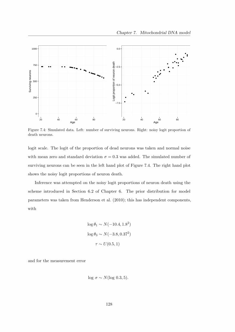
Chapter 7. Mitochondrial DNA model
●● ● ● ● ● ●●●● ●● ●●●●●
●●●●●● ●●●●●●
●●●●●
●●
0
250
500
750
1000
20 40 60 80Age
Sur
vivi
ng n
euro
ns
●
●
●●
●
●
●
●
●
●
●
●
●
●
●
●●
●
●●
●
●
●●
●
●
●
●
●
●●
●
●
●●●
−7.5
−5.0
−2.5
0.0
20 40 60 80Age
Logi
t pro
port
ion
of n
euro
n de
ath
Figure 7.4: Simulated data. Left: number of surviving neurons. Right: noisy logit proportion ofdeath neurons.
logit scale. The logit of the proportion of dead neurons was taken and normal noise
with mean zero and standard deviation σ = 0.3 was added. The simulated number of
surviving neurons can be seen in the left hand plot of Figure 7.4. The right hand plot
shows the noisy logit proportions of neuron death.
Inference was attempted on the noisy logit proportions of neuron death using the
scheme introduced in Section 6.2 of Chapter 6. The prior distribution for model
parameters was taken from Henderson et al. (2010); this has independent components,
with
log θ1 ∼ N(−10.4, 1.82)
log θ3 ∼ N(−3.8, 0.372)
τ ∼ U(0.5, 1)
and for the measurement error
log σ ∼ N(log 0.3, 5).
128

Chapter 7. Mitochondrial DNA model
The MCMC scheme was run for 100K iterations, then the sample was thinned,
keeping every 10th iteration. The trace plots and autocorrelation plots shown in the
middle and right hand panels of Figure 7.5 suggest convergence has been achieved.
Histograms of the marginal posterior distributions for the model parameters are
given in the left hand panels of Figure 7.5. The prior distributions are given in red
and the true parameter values are displayed in green. It can be seen that all model
parameter seem to be well recovered.
7.4 Analysis of experimental data
The results of inference using the experimental data on neuron survival given in Table 7.2
can be seen in Figure 7.6. The vertical green lines represent the posterior means
obtained in Henderson et al. (2010), where both the neuron survival data and the
deletion accumulation data were considered.
The details of the inference scheme, including the prior distributions (shown in red)
are the same as for the simulated data. The trace plots and autocorrelation plots in the
middle and right hand panels of Figure 7.6 suggest convergence.
It can be seen that, in general, the analysis returns similar posterior means to that
of Henderson et al. (2010). This is very encouraging since it would be expected that
there is a lot of information in the deletion accumulation data.
A more formal comparison is given in Table 7.3. The first column shows the posterior
means and 95% equal-tailed posterior probability intervals obtained from Henderson
et al. (2009), when only the deletion accumulation data was used (D1). The second
column shows the equivalent information taken from Henderson et al. (2010), when the
deletion accumulation and the neuron survival data were used (D2). The third column
shows the results of the analysis from this chapter, when only the neuron survival data
was used (D3).
It can be seen that for all parameters, the analysis using D3 gives wider intervals than
the analysis using D2. This is perhaps not surprising, however, it is encouraging to note
129

Chapter 7. Mitochondrial DNA model
log θ1
0.0
0.5
1.0
−14 −12 −10 −8log θ1
Den
sity
log θ1
−11.5
−11.0
−10.5
−10.0
0 5000 10000Index
log
θ 1
log θ1
0.00
0.25
0.50
0.75
1.00
0 100 200 300 400Lag
AC
F
log θ3
0.00
0.25
0.50
0.75
1.00
1.25
−5 −4 −3log θ3
Den
sity
log θ3
−5.5
−5.0
−4.5
−4.0
−3.5
0 5000 10000Index
log
θ 3
log θ3
0.00
0.25
0.50
0.75
1.00
0 100 200 300 400Lag
AC
F
τ
0
5
10
0.5 0.6 0.7 0.8 0.9 1.0τ
Den
sity
τ
0.7
0.8
0.9
1.0
0 5000 10000Index
τ
τ
0.00
0.25
0.50
0.75
1.00
0 100 200 300 400Lag
AC
F
log σ
0.0
0.5
1.0
1.5
2.0
−2.0 −1.5 −1.0 −0.5 0.0log σ
Den
sity
log σ
−1.5
−1.0
−0.5
0 5000 10000Index
log
σ
log σ
0.00
0.25
0.50
0.75
1.00
0 100 200 300 400Lag
AC
F
Figure 7.5: Results of parameter inference on model parameters for the mtDNA model usingsimulated data.
130
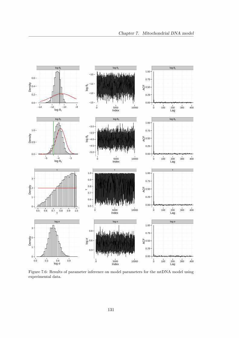
Chapter 7. Mitochondrial DNA model
log θ1
0.0
0.2
0.4
0.6
−14 −12 −10 −8log θ1
Den
sity
log θ1
−13
−12
−11
−10
0 5000 10000Index
log
θ 1
log θ1
0.00
0.25
0.50
0.75
1.00
0 100 200 300 400Lag
AC
F
log θ3
0.0
0.5
1.0
−5 −4 −3log θ3
Den
sity
log θ3
−5.0
−4.5
−4.0
−3.5
−3.0
0 5000 10000Index
log
θ 3
log θ3
0.00
0.25
0.50
0.75
1.00
0 100 200 300 400Lag
AC
F
τ
0
1
2
3
0.5 0.6 0.7 0.8 0.9 1.0τ
Den
sity
τ
0.5
0.6
0.7
0.8
0.9
1.0
0 5000 10000Index
τ
τ
0.00
0.25
0.50
0.75
1.00
0 100 200 300 400Lag
AC
F
log σ
0
1
2
3
0.0 0.3 0.6 0.9log σ
Den
sity
log σ
0.3
0.6
0.9
0 5000 10000Index
log
σ
log σ
0.00
0.25
0.50
0.75
1.00
0 100 200 300 400Lag
AC
F
Figure 7.6: Results of parameter inference on model parameters for the mtDNA model usingexperimental data.
131

Chapter 7. Mitochondrial DNA model
D1 D2 D3
Deletion accumulation Deletion accumulation data Neuron survivaldata only and neuron survival data data only
log θ1 −10.18 (−10.57,−9.79) −10.74 (−10.94,−10.55) −11.15 (−12.18,−10.22)log θ3 −4.51 (−5.09,−3.92) −4.39 (−4.95,−3.91) −4.00 (−4.60,−3.40)τ 0.962 (0.868, 0.999) 0.981 (0.930, 0.999) 0.83 (0.59, 0.993)
Table 7.3: Posterior means and 95% equal-tailed posterior probability intervals (in parenthesis),for inference using different datasets.
that the posterior means from the D2 analysis all lie well within the 95% equal-tailed
posterior probability intervals for the D3 analysis.
This is also the case when comparing the D1 analysis with the D3 analysis, apart
from the log θ1 parameter where the posterior mean obtained in the D1 analysis of
-10.18 lies slightly outside of the posterior interval of (−12.18,−10.22) obtained from
the D3 analysis.
Figure 7.7 shows a plausible range of logit proportions determined via 99% predictive
intervals for each age. The intervals were constructed by taking 300 samples from the
posterior distribution then simulating a dataset from the model using each of these
parameter sets. The central 99% of these simulations is plotted (light grey). The crosses
on the plot represent the experimental data. It can be seen that in general, this interval
gives good coverage of the experimental data suggesting that the parameter choices
found are consistent with the data.
7.5 Conclusions
Previous attempts to calibrate the mtDNA model have been successful, however, no
attempts have been made using only the neuron survival data presented in Table 7.2.
In this chapter, inference has successfully been performed for the model parameters of
the mtDNA model using the neuron survival data, along with a comparable synthetic
dataset.
Firstly, analysis of a synthetic dataset where the true parameters were known was
132

Chapter 7. Mitochondrial DNA model
−12
−8
−4
0
4
20 40 60 80Age
Logi
t pro
port
ion
of n
euro
n de
ath
Figure 7.7: Plausible range of logit proportions determined via 99% predictive intervals for eachage.
attempted. This resulted in marginal posterior distributions which were centred around
their true parameter values and significant information was learned from the prior
distribution.
Next, analysis of the neuron survival data was attempted. The resulting marginal
posterior distributions were consistent with that of Henderson et al. (2010). This was
encouraging since, unlike Henderson et al. (2010), no observations on the underlying
chemical species were included. The predictive posterior distribution demonstrates that
the posterior distributions for model parameters are consistent with the experimental
data. However, two notable improvement which could be made to the model are to
include a mechanism which recognises the binomial sampling error in the data and to
include prior information on the initial number of neurons at birth, N . This could be
implemented by adding an extra input to the design space of the emulator.
133

Chapter 8
PolyQ model
8.1 Introduction
The PolyQ model, developed by Tang et al. (2010), is a large stochastic kinetic model
capturing biological processes at the molecular level within human cells as they undergo
ageing. Modelling and understanding these processes are important for the treatment
of neurodegenerative diseases such as Huntington’s disease.
The model was introduced in Chapter 2, where a brief background was given along
with some example simulations. The model contains 25 chemical species which are
listed in Table 2.4. These chemical species typically represent numbers of molecules
of a particular protein which can react through a series of reactions. There are 69
reactions each of which will typically involve an increase or decrease in the number
of molecules of a certain protein. A list of reactions was given in Table 2.5 along
with the associated rates. s The model is represented graphically in Figure 8.1. Oval
shapes (nodes) represent chemical species and an arrow between two nodes represents
a reaction which can take place involving the two chemical species. It is not intended
that this network diagram should be studied in detail, rather that it gives the reader an
impression of the size and complexity of the model.
134

Chapter 8. PolyQ model
Fig
ure
8.1:
Net
work
dia
gra
mof
react
ion
sin
the
Poly
Qm
od
el
135

Chapter 8. PolyQ model
Current research is based on fixing the parameters in the model at the expert’s best
guesses and then manually adjusting them to match experimental data. This chapter
considers parameter inference for parameters in the PolyQ model using two different
synthetic datasets on proportions of cell death.
The number of parameters in the PolyQ model is large and attempting to make
inference on all 40 parameters would be a very ambitious task. Since in previous
chapters, inference on a maximum of three model parameters (plus measurement error)
has been considered, it was decided that this should be extended to four parameters for
the PolyQ model. In conjunction with the mathematical modellers, the four parameters
were chosen which are most important for cell death and inference was considered for
these parameters; all other parameters values were fixed at the expert’s best guess. Since
the model is slow to simulate from, Gaussian process emulators are built for proportions
of cell death. These emulators are then embedded into inference schemes.
8.2 The stochastic model
A full list of the 25 chemical species in the model is given in Table 2.4 of Chapter 2.
The initial number of each chemical species assumed by Tang et al. (2010) is also given.
Table 8.1 is a condensed version of Table 2.4 containing only the chemical species which
will be of direct interest for the analysis in this chapter. Table 2.5 of Chapter 2 contains
a full list of all reactions which can take place in the model. A condensed version of
this table is given in Table 8.2, which includes only the reactions whose rates involve
the four parameters included in this analysis.
Some further biological details are given below on the parts of the model which are
directly related to the parameters of interest in this chapter. However, it must be noted
that there are many more processes happening in the model which are not discussed
below.
136

Chapter 8. PolyQ model
Name Description Initial amount
Proteasome 26S Proteasome 1000AggPolyQi PolyQ aggregate of size i (i = 1, . . . , 5) 0AggPProteasome Aggregated protein bound to proteasome 0ROS Reactive oxygen species 10p38P Active P38MAPK 0p38 Inactive p38MAPK 100AggPi Small aggregate of size i (i = 1, . . . , 5) 0PIdeath Dummy species to record cell death due to proteasome inhibition 0p38death Dummy species to record cell death due to p38MAPK activation 0
Table 8.1: List of species
ID Reaction name Reaction Rate law
17a Proteasome inhibition AggPolyQ1 + Proteasome → kinhprot[AggPPolyQ1][Proteasome]AggPProteasome
17b AggPolyQ2 + Proteasome → kinhprot[AggPPolyQ2][Proteasome]AggPProteasome
17c AggPolyQ3 + Proteasome → kinhprot[AggPPolyQ3][Proteasome]AggPProteasome
17d AggPolyQ4 + Proteasome → kinhprot[AggPPolyQ4][Proteasome]AggPProteasome
17e AggPolyQ5 + Proteasome → kinhprot[AggPPolyQ5][Proteasome]AggPProteasome
37a AggP1 + Proteasome → kinhprot[AggP1][Proteasome]AggPProteasome
37b AggP2 + Proteasome → kinhprot[AggP2][Proteasome]AggPProteasome
37c AggP3 + Proteasome → kinhprot[AggP3][Proteasome]AggPProteasome
37d AggP4 + Proteasome→ kinhprot[AggP4][Proteasome]AggPProteasome
37e AggP5 + Proteasome → kinhprot[AggP5][Proteasome]AggPProteasome
20a ROS generation AggPolyQ1 → AggPolyQ1 + ROS kgenROSAggP [AggPolyQ1]20b AggPolyQ2 → AggPolyQ2 + ROS kgenROSAggP [AggPolyQ2]20c AggPolyQ3 → AggPolyQ3 + ROS kgenROSAggP [AggPolyQ3]20d AggPolyQ4 → AggPolyQ4 + ROS kgenROSAggP [AggPolyQ4]20e AggPolyQ5 → AggPolyQ5 + ROS kgenROSAggP [AggPolyQ5]21 AggPProteasome kgenROSAggP [AppPProteasome]
→ AggPProteasome + ROS
38a AggP1 → AggP1 + ROS kgenROSAggP [AggP1]38b AggP2 → AggP2 + ROS kgenROSAggP [AggP2]38c AggP3 → AggP3 + ROS kgenROSAggP [AggP3]38d AggP4 → AggP4 + ROS kgenROSAggP [AggP4]38e AggP5 → AggP5 + ROS kgenROSAggP [AggP5]39 p38P → p38P + ROS kgenROSp38 ∗ kp38act[p38P]22 p38MAPK activation ROS + p38 → ROS + p38P kactp38[ROS][p38]41 p38 cell death p38P → p38P + p38death kp38deathkp38act[p38P]42 PI cell death AggPProteasome → kpIdeath[AggPProteasome]
AggPProteasome + pIdeath
Table 8.2: List of reactions and hazards for the PolyQ model
137

Chapter 8. PolyQ model
AggP and AggPolyQ
The AggPi represent small aggregates of proteins of size i where i = 1, . . . , 5. For example,
AggP1 represents aggregates of proteins of size one. The formation of these aggregates is
due to presence of misfolded proteins in the cell. In the model, the production of these
aggregates is encoded using a set of reactions whereby an aggregate of AggPi binds to a
misfolded protein producing an aggregate of AggPi+1.
Similarly, the AggPolyQi represent aggregates of PolyQ proteins of size i (i = 1, . . . , 5)
where i = 1, . . . , 5. PolyQ aggregates are formed when PolyQ proteins clump together.
ROS
Reactive oxygen species (ROS) are molecules of oxygen with an unpaired electron, making
them very reactive. The generation of ROS as a by product of reactions involving
oxygen is normal in all cells, however, increased levels of ROS can be dangerous, putting
the cell under oxidative stress. Increased levels of ROS in neurons is a typical feature of
age-related neurodegenerative disease such as Huntington’s disease.
It can be seen from Table 8.2, that ROS is produced as a result of protein aggregation
(reactions 20a–20e, 21, 38a–38e) and due to the production of p38P (reaction 39).
Proteasome
The proteasome are protein complexes found in the nucleus of all eukaryotic cells. The
purpose of the proteasome is to break down and remove damaged and misfolded proteins
in the cell. If the proteasome are not able to do their job, the cell is put under stress.
Inhibition of the proteasome can ultimately cause a chain of reactions which leads to
cell death.
Reactions 17a–e and 37a–e of Table 8.2 describe the process of protein aggregates
(either AggPi or AggPolyQi) inhibiting the proteasome (represented by AggPProteasome).
Reaction 42 is the mechanism for cell death due to proteasome inhibition. This reaction
is more likely to happen when there are high levels of AggPProteasome.
138

Chapter 8. PolyQ model
p38 and p38P
p38MAPK (mitogen-activated protein kinases) are part of a class of proteins within the
cell which are responsible for regulating processes such as gene expression and mitosis.
In the PolyQ model, p38 represents inactive p38MAPK and p38P and represent active
p38MAPK.
When PolyQ proteins are being produced in a cell, p38MAPK is known to play a
role in cell death. Tang et al. (2010) conclude that the inhibition of p38MAPK, reduces
cell death due to this pathway.
In the PolyQ model, cells are assumed to have an initial number of 100 molecules of
inactive p38MAPK (p38). It can be seen in reaction 22 of Table 8.2 that high levels of
ROS increase the likelihood of p38MAPK activation. Cell death is more likely to occur
in the model for high levels of p38MAPK activation. The dummy species p38death is
included in the model as a binary variable. While the cell is alive, p38death = 0 and if
cell death occurs via this pathway, p38death = 1.
Model parameters
A full list of parameters in the PolyQ model is given in Table 8.3 along with their
current values, which are the modellers best guesses. There are four model parameters
that will be considered in the analysis in this chapter which are highlighted in colour in
the table. These are
• kinhprot: controls the rate of proteasome inhibition which leads to cell death.
Features in 10 of reactions in Table 2.5 and is highlighted in red.
• kgenROSAggP : controls the amount of ROS produced after stress which leads to
the activation of p38 and cell death. Features in 11 reactions in Table 2.5 and is
highlighted in blue.
• kgenROSp38: Similar function to kgenROSAggP . This parameter features in reaction
39 and is highlighted in green.
139

Chapter 8. PolyQ model
Parameter Value Parameter Value
kaggPolyQ 5.0× 10⁻⁸ kgenROS 1.7× 10⁻³
kdisaggPolyQ1 5.0× 10⁻⁷ kremROS 2.0× 10⁻⁴
kdisaggPolyQ2 4.0× 10⁻⁷ kgenROSAggP 5.0× 10⁻⁶
kdisaggPolyQ3 3.0× 10⁻⁷ kgenROSSeqAggP 1.0× 10⁻⁷
kdisaggPolyQ4 2.0× 10⁻⁷ kactp38 5.0× 10⁻⁶
kdisaggPolyQ5 1.0× 10⁻⁷ kinactp38 2.0× 10⁻³
kseqPolyQ 8.0× 10⁻⁷ kseqMisP 1.0× 10⁻⁹
kinhprot 5.0× 10⁻⁹ kseqAggPProt 5.0× 10⁻⁷
kaggMisP 1.0× 10⁻¹¹ kseqPolyQProt 5.0× 10⁻⁷
kagg2MisP 1.0× 10⁻¹⁰ kseqMisPProt 5.0× 10⁻⁷
kdisaggMisP1 5.0× 10⁻⁷ kseqmRFPuProt 5.0× 10⁻⁷
kdisaggMisP2 4.0× 10⁻⁷ kseqmRFPu 1.0× 10⁻¹⁰
kdisaggMisP3 3.0× 10⁻⁷ ksynNatP 2.4kdisaggMisP4 2.0× 10⁻⁷ kmisfold 2.0× 10⁻⁶
kdisaggMisP5 1.0× 10⁻⁷ krefold 8.0× 10⁻⁵
ksynmRFPu 1.38× 10⁻¹ kbinMisPProt 5.0× 10⁻⁸
kbinmRFPu 5.0× 10⁻⁷ krelMisPProt 1.0× 10⁻⁸
krelmRFPu 1.0× 10⁻⁸ kdegMisP 1.0× 10⁻²
kdegmRFPu 5.0× 10⁻³ kgenROSp38 7.0× 10⁻⁴
ksynPolyQ 7.0× 10⁻³ kp38act 1kbinPolyQ 5.0× 10⁻⁸ kPIdeath 2.5× 10⁻⁸
krelPolyQ 1.0× 10⁻⁹ kproteff 1.0kdegPolyQ 2.5× 10⁻³ kalive 1.0
Table 8.3: PolyQ parameters and the values used for simulating data.
• kkactp38: controls the rate at which p38 is activated leading to cell death. Features
in reaction 22 and is highlighted in purple.
For notation simplicity the following reparametrisation will be used
θ1 = log kinhprot, θ2 = log kgenROSAggP , θ3 = log kgenROSp38, θ4 = log kactp38.
8.3 Experimental data
The experimentalists start off with a large number of cells and use a technique called
propidium iodide exclusion to identify the viability (death status) of the cells over
time. The cells are treated and then stained with propidium iodide, a fluorescent dye.
Propidium iodide has the property of only binding to non-viable cells. The fluorescent
140
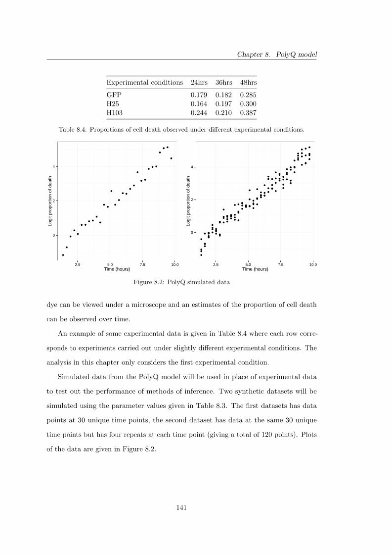
Chapter 8. PolyQ model
Experimental conditions 24hrs 36hrs 48hrs
GFP 0.179 0.182 0.285H25 0.164 0.197 0.300H103 0.244 0.210 0.387
Table 8.4: Proportions of cell death observed under different experimental conditions.
●
●
●
●
●
● ●
● ●
●
●
●●
●
●
●
● ●
●
●
●
● ●
●● ●
●
● ●
●
0
2
4
2.5 5.0 7.5 10.0Time (hours)
Logi
t pro
port
ion
of d
eath
●
●
●
●
●
● ●
● ●
●
●
●●
●
●
●
● ●
●
●
●
● ●
●● ●
●
● ●
●
●
● ●
●
●
●
●
●
●
●
●
●
● ●
●●
● ●
●
●
● ●●
●
●
●
●
●
●
●
●
●
●
●
●●
●
● ●
●
●
●●
●
●
●
●
●
●●
●
●
●
●
●●
●
●●
●
●
●
●
●
●
●
● ● ● ●
●
●
● ●● ●
● ●
●
●●
●
●
●
●
● ●
● ● ●
0
2
4
2.5 5.0 7.5 10.0Time (hours)
Logi
t pro
port
ion
of d
eath
Figure 8.2: PolyQ simulated data
dye can be viewed under a microscope and an estimates of the proportion of cell death
can be observed over time.
An example of some experimental data is given in Table 8.4 where each row corre-
sponds to experiments carried out under slightly different experimental conditions. The
analysis in this chapter only considers the first experimental condition.
Simulated data from the PolyQ model will be used in place of experimental data
to test out the performance of methods of inference. Two synthetic datasets will be
simulated using the parameter values given in Table 8.3. The first datasets has data
points at 30 unique time points, the second dataset has data at the same 30 unique
time points but has four repeats at each time point (giving a total of 120 points). Plots
of the data are given in Figure 8.2.
141

Chapter 8. PolyQ model
8.4 Emulating proportions of death from the PolyQ model
Emulators will be built for the PolyQ model using the framework developed in previous
chapters. For both synthetic datasets, there are observations at 30 unique time points.
Consequently, a emulator will be built for the logit proportions of cell death at each of
the 30 time points.
8.4.1 Mean function and covariance function
As with the mtDNA model, multiple linear regression was performed to advise the
choice of mean function. Terms were added sequentially, starting with the linear terms,
then adding squared terms and interactions. Any non–significant terms were discarded
and the final mean function was
m(θ1, θ2, θ3, θ4) = β0 + β1θ1 + β2θ2 + β3θ3 + β4θ4 + β5θ21 + β6θ
22 + β7θ
23 + β8θ
24+
β9θ1θ2 + β10θ1θ3 + β11θ1θ2θ3 + β12θ1θ2θ4 + β13θ1θ2θ3θ4,
where the βi are the least square estimates from the regression. The squared exponential
covariance function will take the form
K(θi,θj |a, r) = a exp
{−(
(θi1 − θj1)2
r21+
(θi2 − θj2)2
r22+
(θi3 − θj3)2
r23+
(θi4 − θj4)2
r24
)}.
The five hyperparameters (a, r1, r2, r3, r4) will be estimated from the training data.
142

Chapter 8. PolyQ model
8.4.2 Training data
Model parameters were thought to be independent a priori and chosen to represent
fairly vague prior knowledge, with
θ1 ∼ N(log 5× 10⁻⁹, 5)
θ2 ∼ N(log 5× 10⁻⁶, 5)
θ3 ∼ N(log 7× 10⁻⁴, 5)
θ4 ∼ N(log 5× 10⁻⁶, 5).
The emulators were fitted using a Latin hypercube design with nd = 1000 points
distributed over the middle 95% of these prior distributions using the maximin design
introduced in Chapter 5. The HTCondor system which was described in Chapter 7 was
used to obtain the training runs. In total, this took less than 24 hours.
8.4.3 Estimating hyperparameters and diagnostics
The prior distributions used for hyperparameters were assumed to be independent a
priori, where
a ∼ Log-Normal(0, 100) and ri ∼ Log-Normal(0, 100) for i = 1, 2, 3, 4,
and represent vague prior knowledge about hyperparameters. The marginal posterior
distributions for hyperparameters can be seen in Figure 8.3 where the five panels
represent the five hyperparameters estimated using the scheme in Algorithm 13 of
Chapter 5. The prior distributions can be seen in red, clearly the training data has been
very informative. There appears to be a gradual shift in the posterior distributions for
hyperparameters across time. In particular, the posterior mean for the log a parameter
increases from approximately −0.75 at time 0 to approximately 0.25 at time 20. This
suggests that the variance on the proportions of cell death increases with time – as
would be expected.
143

Chapter 8. PolyQ model
Due to the relatively large size of Latin hypercube required for this model, it takes
around one day to run each scheme for 1000 iterations, of which there are 30 emulators.
Since fitting each emulator is independent of all other, the HTCondor system can be
used to parallelise this task.
Diagnostics for the emulators can be seen in Figure 8.4. These diagnostics were
constructed using a validation dataset generated using another maximin Latin hypercube
covering the same range as the original containing nd† = 100 points. The diagnostics
seem to be reasonable, suggesting that in general the emulators are fitting acceptably.
Some of the Mahalanobis distances are slightly higher than would be expected, especially
for emulators at times 20 – 30, however, the IPE and PIT histograms look satisfactory
for these emulators.
8.5 Analysis of simulated data
The results of analysis of simulated data can be seen for the dataset with 30 points in
Figure 8.5 and for the dataset with 120 points in Figure 8.6. For each analysis, the
MCMC scheme was run for 10K iterations and samples were thinned such that every
10th iteration was kept. The marginal posterior distributions are given in black and
the prior distributions in red. The trace plots and autocorrelation plots are given in
the middle and right hand panels of each figure. These suggest convergence has been
achieved for both schemes.
144
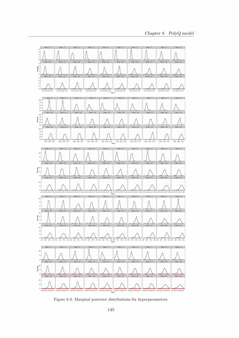
Chapter 8. PolyQ model
Time = 0 Time = 1 Time = 2 Time = 3 Time = 4 Time = 5 Time = 6 Time = 7 Time = 8 Time = 9
Time = 10 Time = 11 Time = 12 Time = 13 Time = 14 Time = 15 Time = 16 Time = 17 Time = 18 Time = 19
Time = 20 Time = 21 Time = 22 Time = 23 Time = 24 Time = 25 Time = 26 Time = 27 Time = 28 Time = 29
0
1
2
3
4
0
1
2
3
4
0
1
2
3
4
−1.0−0.5 0.0 0.5 −1.0−0.5 0.0 0.5 −1.0−0.5 0.0 0.5 −1.0−0.5 0.0 0.5 −1.0−0.5 0.0 0.5 −1.0−0.5 0.0 0.5 −1.0−0.5 0.0 0.5 −1.0−0.5 0.0 0.5 −1.0−0.5 0.0 0.5 −1.0−0.5 0.0 0.5log a
dens
ity
Time = 0 Time = 1 Time = 2 Time = 3 Time = 4 Time = 5 Time = 6 Time = 7 Time = 8 Time = 9
Time = 10 Time = 11 Time = 12 Time = 13 Time = 14 Time = 15 Time = 16 Time = 17 Time = 18 Time = 19
Time = 20 Time = 21 Time = 22 Time = 23 Time = 24 Time = 25 Time = 26 Time = 27 Time = 28 Time = 29
0.0
2.5
5.0
7.5
10.0
0.0
2.5
5.0
7.5
10.0
0.0
2.5
5.0
7.5
10.0
1.25 1.50 1.75 1.25 1.50 1.75 1.25 1.50 1.75 1.25 1.50 1.75 1.25 1.50 1.75 1.25 1.50 1.75 1.25 1.50 1.75 1.25 1.50 1.75 1.25 1.50 1.75 1.25 1.50 1.75log r1
Den
sity
Time = 0 Time = 1 Time = 2 Time = 3 Time = 4 Time = 5 Time = 6 Time = 7 Time = 8 Time = 9
Time = 10 Time = 11 Time = 12 Time = 13 Time = 14 Time = 15 Time = 16 Time = 17 Time = 18 Time = 19
Time = 20 Time = 21 Time = 22 Time = 23 Time = 24 Time = 25 Time = 26 Time = 27 Time = 28 Time = 29
0
5
10
0
5
10
0
5
10
1.3 1.4 1.5 1.6 1.7 1.8 1.3 1.4 1.5 1.6 1.7 1.8 1.3 1.4 1.5 1.6 1.7 1.8 1.3 1.4 1.5 1.6 1.7 1.8 1.3 1.4 1.5 1.6 1.7 1.8 1.3 1.4 1.5 1.6 1.7 1.8 1.3 1.4 1.5 1.6 1.7 1.8 1.3 1.4 1.5 1.6 1.7 1.8 1.3 1.4 1.5 1.6 1.7 1.8 1.3 1.4 1.5 1.6 1.7 1.8log r2
Den
sity
Time = 0 Time = 1 Time = 2 Time = 3 Time = 4 Time = 5 Time = 6 Time = 7 Time = 8 Time = 9
Time = 10 Time = 11 Time = 12 Time = 13 Time = 14 Time = 15 Time = 16 Time = 17 Time = 18 Time = 19
Time = 20 Time = 21 Time = 22 Time = 23 Time = 24 Time = 25 Time = 26 Time = 27 Time = 28 Time = 29
0
4
8
12
0
4
8
12
0
4
8
12
0.4 0.6 0.8 1.0 0.4 0.6 0.8 1.0 0.4 0.6 0.8 1.0 0.4 0.6 0.8 1.0 0.4 0.6 0.8 1.0 0.4 0.6 0.8 1.0 0.4 0.6 0.8 1.0 0.4 0.6 0.8 1.0 0.4 0.6 0.8 1.0 0.4 0.6 0.8 1.0log r3
Den
sity
Time = 0 Time = 1 Time = 2 Time = 3 Time = 4 Time = 5 Time = 6 Time = 7 Time = 8 Time = 9
Time = 10 Time = 11 Time = 12 Time = 13 Time = 14 Time = 15 Time = 16 Time = 17 Time = 18 Time = 19
Time = 20 Time = 21 Time = 22 Time = 23 Time = 24 Time = 25 Time = 26 Time = 27 Time = 28 Time = 29
0
5
10
0
5
10
0
5
10
0.5 0.6 0.7 0.8 0.9 1.0 0.5 0.6 0.7 0.8 0.9 1.0 0.5 0.6 0.7 0.8 0.9 1.0 0.5 0.6 0.7 0.8 0.9 1.0 0.5 0.6 0.7 0.8 0.9 1.0 0.5 0.6 0.7 0.8 0.9 1.0 0.5 0.6 0.7 0.8 0.9 1.0 0.5 0.6 0.7 0.8 0.9 1.0 0.5 0.6 0.7 0.8 0.9 1.0 0.5 0.6 0.7 0.8 0.9 1.0log r4
Den
sity
Figure 8.3: Marginal posterior distributions for hyperparameters.
145

Chapter 8. PolyQ model
●
●
●
●●●
●●●
●
●
●
●
●●●
●●●●●
●●●
●
●
●
●
●
●
●●●●
●
●
●
●●
●
●●
●
●
●
●
●●●
●
●●●
●
●●
●
●
●
●
●
●
●
●
●●
●
●
●
●●●
●
●
●
●
●●●●●
●●●●
●
●
●●●
●●
●
●
●●●●●
●
●
●●●
●●●
●●
●●
●
●
●●●
●●●●
●
●
●●
●
●
●●●
●
●●
●
●
●
●●
●
●
●
●●●
●
●●●
●
●
●
●
●
●
●
●●
●
●
●
●●●●●●
●
●●●●●
●●●●
●●
●●●
●●●
●
●●●●
●●
●
●●●
●
●●●●
●●
●
●
●●●
●●
●
●
●
●●●
●
●●●●●
●
●
●
●
●
●●
●
●
●
●●●●●●●
●
●
●●●
●
●
●●●
●
●●●●
●●●●●●
●●
●●●●
●●●
●●●●●●
●
●
●
●●
●
●
●
●●●
●
●●
●●
●●
●
●●
●●
●●
●
●
●
●●●
●●
●●●●
●
●
●●
●●●●
●
●
●●●
●
●●
●●
●
●●●
●
●
●●●
●
●
●●●
●●
●●●
●
●
●●●
●●●●●
●●●●●●
●
●
●
●●
●●
●
●
●●
●
●●
●●
●●
●
●●
●
●
●●●●●
●
●●●●
●
●●
●
●
●
●●
●●
●●
●●●●●
●
●●●●
●
●●●
●
●
●●●
●
●
●●
●
●●
●●●
●
●
●●●●●●●●
●●● ●
●●
●
●
●
●●●●
●
●●●
●
●
●
●●
●●
●
●●
●
●
●●●●●
●
●
●●●
●●●
●●●
●●
●●
●●
●
●
●●●●●●●●
●
●●●
●
●
●
●●
●
●
●●
●
●
●●●●
●
●●●
●●●●●●
●●●
●
●●
●
●
●
●●
●●
●
●●●
●●
●
●●
●●
●
●●
●
●
●●
●●●●
●
●●●●●●
●●
●
●●●●
●●
●●
●●●
●
●●●
●
●
●●●
●
●
●
●●
●
●
●
●
●
●
●●●●
●
●●●●●●●●●
●●● ●
●●●
●
●
●●
●
●
●
●●
●●●
●
●●
●●
●
●●
●
●
●
●
●●●●
●
●●●●●●
●●●
●●●●
●●
●●
●●●
●
●●●
●
●
●●
●
●
●
●●●
●●●●●
●●●
●
●
●
●●●●●●
●
●●
●●●●
●
●●
●
●
●●
●
●
●
●●●●
●
●
●
●
●●
●
●●●
●
●
●
●●●●
●
●●●
●●●
●●
●
●●●●
●●
●●
●●
●
●
●
●●
●
●
●●
●
●
●
●●
●
●●●
●
●●●●
●
●
●
●●●
●●●●●●
●●● ●
●●●
●●●●●
●●
●●
●●
●
●
●
●
●●
●
●●
●
●
●
●
●●●●
●
●●●
●●
●
●●
●
●●
●●
●●
●●
●●
●
●
●
●●
●
●
●●●
●
●
●●
●
●●●
●
●●●●●
●●●●
●
●●●
●
●
●
●●
●
●●●●
●
●
●
●●
●●
●●●●●●
●
●
●●
●
●●●
●
●
●
●
●●●
●
●●●
●●●
●●●
●●●●
●●
●●●
●
●●
●
●●
●
●
●●
●
●●
●●●
●●●
●
●●●●●
●●●●●●●●●●
●
●●
●
●
●●
●
●
●●●
●
●
●●
●
●●●●●●●●
●●
●
●
●
●●
●
●
●
●
●
●●●
●
●●
●
●●
●●
●
●
●●
●
●●
●
●●
●
●
●●
●
●●
●
●●
●
●●
●●●
●●●●●●
●●●●●●●●●
●
●
●●
●●
●●
●●
●●●
●
●
●●
●
●●●
●
●●●●
●●
●
●
●
●
●
●●●
●
●
●●
●
●
●●
●●●
●●
●●
●
●
●●
●
●
●●
●
●
●●
●
●●
●
●●
●
●●●●●●●●●●●●●●●●●●●●
●
●●●●
●●●
●●
●●●●
●
●●
●●
●●
●
●●
●●●●
●●
●
●●
●
●●●●
●●
●
●●●
●
●●
●●●●
●
●
●●
●●
●●
●
●●●
●
●●
●
●●
●
●●
●●●●●●●●●●
●
●
●
●
●●●●
●
●●●●
●
●●
●●
●
●●
●
●
●●
●●
●●
●
●●
●●
●●●
●●
●●
●●●●●●●●
●
●●●
●
●
●
●
●
●
●
●
●●
●●
●●
●
●●●
●
●●
●
●●
●
●●●●●●●●●●●●
●●
●
●●●●●
●
●
●●●
●
●●
●●
●●
●●
●
●
●
●●
●●
●
●●
●●
●●
●
●
●
●
●
●●●
●●●●●
●●●●
●
●
●●
●
●
●
●●●
●
●
●●
●
●●●●
●●
●
●
●
●
●●●●●
●●●
●●●●
●●
●
●●●●●
●
●
●●●
●
●●
●
●●●●
●
●
●
●
●●
●
●
●
●●
●
●
●●
●
●
●
●●
●●●
●●●●●
●●●●
●●
●●●
●
●
●●●
●
●
●●
●
●●●
●
●
●●
●
●
●
●●●●●
●●●
●●●●
●●
●
●●●●●●
●
●●●
●●●●●●●●
●
●
●
●
●
●
●
●
●
●
●●
●●
●
●●
●
●
●
●
●
●
●●●●●
●●●●
●●
●●
●
●
●
●
●●
●
●
●●●●●●
●
●
●
●
●
●
●
●●●●●
●●
●
●●●●●●
●
●●
●
●●●
●
●●●
●
●
●●●●●●
●
●
●
●
●●
●
●
●
●●●
●●
●
●●
●
●●
●
●
●
●●●●●
●●●
●
●●
●●●
●
●
●●●●
●
●●
●●●●●●
●●
●
●
●
●
●
●●●●●
●
●●●●●●
●
●●●
●●●
●
●●● ●
●
●●●●
●●
●
●
●
●
●●●
●
●
●●
●
●●
●
●●
●
●
●
●
●
●
●●●●●
●●●
●●
●
●●●●
●
●●
●●
●
●●
●●
●●●●
●●
●
●
●
●
●●●●●●
●●●●●●●
●
●●
●
●●
●
●
●●●
●
●
●●●●●●
●
●
●
●
●
●
●
●
●
●●
●
●●●
●●
●
●
●
●
●
●
●●●●●
●●●
●●
●
●
●●●
●
●
●
●●
●
●●
●●
●●●●
●●●
●
●
●
●
●●●
●●●●●●●●●
●
●●
●
●●●
●
●●●
●
●
●
●●
●●●
●
●
●
●
●
●
●
●
●
●●●●●●
●●
●
●●
●
●
●
●●●●●
●●●
●
●
●
●●●●
●
●●●●
●
●●
●●
●
●●●●●●
●
●
●
●●
●●
●●●●●●●
●●
●
●●
●
●●
●
●
●
●●●
●
●●●
●●●
●
●
●
●●●
●●
●
●
●
●●
●
●●●
●
●●
●
●
●
●●●●●
●●●
●●
●
●
●
●●
●
●●●●
●
●●
●●
●
●●●
●
●●
●
●
●
●●
●●
●
●●●●●●
●●
●
●
●
●●
●
●
●●●
●
●
●
●●●●●
●
●
●
●
●●●●
●
●
●●●
●
●●●
●
●●
●
●
●
●●●●●
●●●
●●
●
●●●●
●
●●●●
●
●●
●
●
●
●●●
●
●●
●
●
●
●●●●
●
●●●●●●
●●
●
●
●
●
●●
●
●
●●●●
●●
●●●●●
●
●
●
●
●●●●●
●
●
●●●
●●●
●
●●
●
●
●
●●●●●
●●●
●●
●
●
●●●
●
●
●
●●
●
●●
●
●
●
●
●●
●
●●
●
●
●
●●●●
●●●●●●●●●
●
●
●
●
●●
●
●
●●●
●
●
●
●●●●●
●
●
●
●●
●
●●
●
●
●●●
●
●●●
●
●●
●
●
●
●●●●●
●●
●
●●
●
●
●●
●
●
●
●
●●
●
●
●
●
●
●
●
●●●●●
●
●
●
●
●●●
●
●●●●●●●●
●
●
●
●
●●●●●●● ●
●
●●●●●●
●
●
●
●●
●
●●
●
●
●●●●●●●
●
●●
●●
●
●●●●●
●●
●
●
●
●
●
●●
●
●
●
●
●●
●
●●
●
●
●
●●●●●●
●
●
●
●
●●●
●
●●●●●●●●
●
●
●
●
●●●●●●● ●
●
●
●●●●●
●
●
●●●
●
●●
●
●
●●●
●●●●
●
●
●●●●
●●●●●
●●●
●●
●
●●
●
●
●
●
●
●●
●
●●
●
●
●
●●●●●●
●
●
●
●●●●●●●●●●●
●
●
●
●
●
●
●●●●●●● ●
●
●
●●●
●●
●
●
●
●●●●●
●
●
●●●●●
●●
●
●
●●●●
●●
●●●
●●●
●●
●
●●
●
●
●
●
●
●●
●
●●
●
●
●
●
●●●●●
●
●
●
●●●●●●●●●
●●●●
●
●
●
●
●●●●●●● ●
●
●
●●●
●●
●
●
●
●●●●●
●
●
●●●
●●
●●
●
●●●●●
●●●●●
●
●
●
●
●
●
●●
●
●
●
●
●
●●
●
●●●
●
●
●
●●●●●
●
●
●
●●●●
●
●●●
●
●●
●
●
●
●
●
●
●●●●●●●
Time = 01 Time = 02 Time = 03 Time = 04 Time = 05 Time = 06 Time = 07 Time = 08 Time = 09 Time = 10
Time = 11 Time = 12 Time = 13 Time = 14 Time = 15 Time = 16 Time = 17 Time = 18 Time = 19 Time = 20
Time = 21 Time = 22 Time = 23 Time = 24 Time = 25 Time = 26 Time = 27 Time = 28 Time = 29 Time = 30
−5.0
−2.5
0.0
2.5
5.0
−5.0
−2.5
0.0
2.5
5.0
−5.0
−2.5
0.0
2.5
5.0
Index
Indi
vidu
al P
redi
ctio
n E
rror
s
Time = 01 Time = 02 Time = 03 Time = 04 Time = 05 Time = 06 Time = 07 Time = 08 Time = 09 Time = 10
Time = 11 Time = 12 Time = 13 Time = 14 Time = 15 Time = 16 Time = 17 Time = 18 Time = 19 Time = 20
Time = 21 Time = 22 Time = 23 Time = 24 Time = 25 Time = 26 Time = 27 Time = 28 Time = 29 Time = 30
0.0
0.5
1.0
1.5
0.0
0.5
1.0
1.5
0.0
0.5
1.0
1.5
0 1 0 1 0 1 0 1 0 1 0 1 0 1 0 1 0 1 0 1Probability Integral Transform, Φ(IPE)
Den
sity
●
●
●● ●
●
●
●
●
●
● ●● ●
● ●●
●
●●
●●
●●
●●
●●
● ●
0
50
100
150
200
250
0 10 20 30Time
Mah
alan
obis
Dis
tanc
e
Figure 8.4: Diagnostics for emulators for the PolyQ model.
146
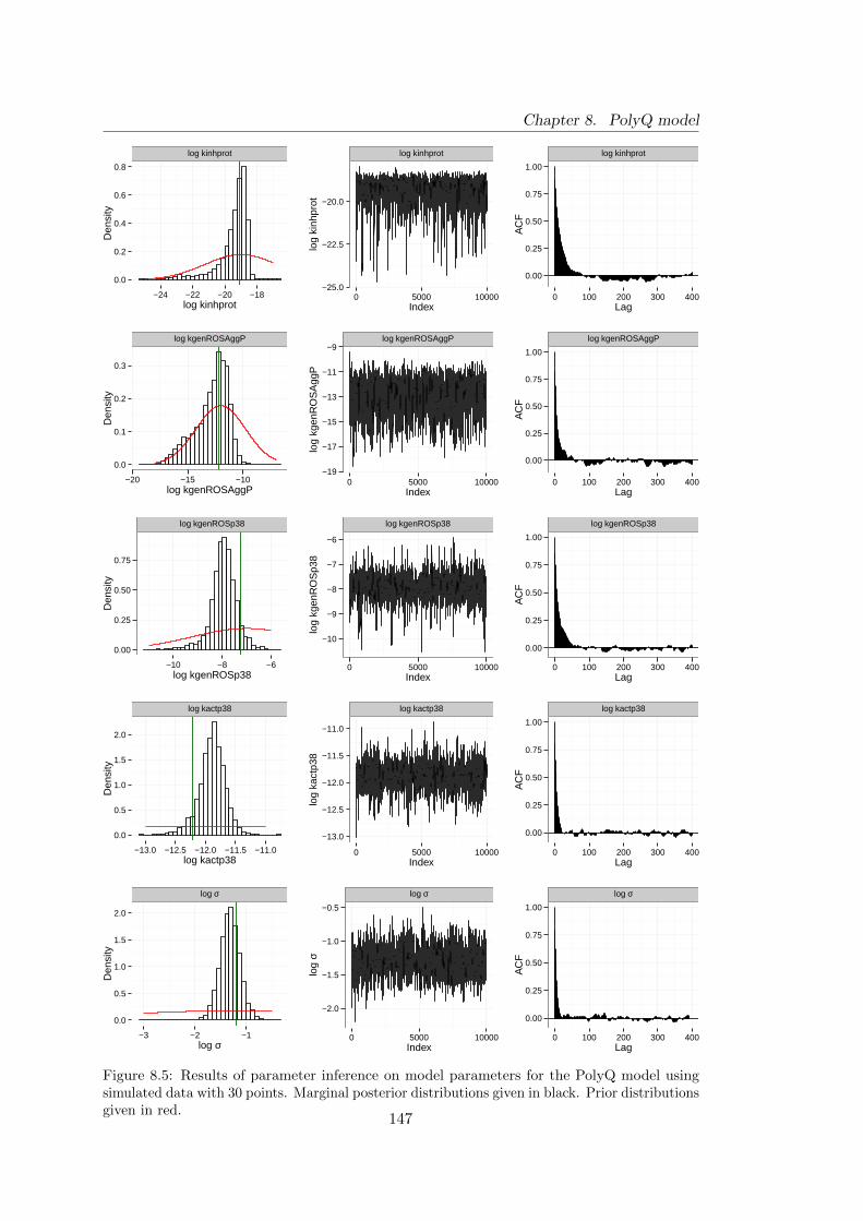
Chapter 8. PolyQ model
log kinhprot
0.0
0.2
0.4
0.6
0.8
−24 −22 −20 −18log kinhprot
Den
sity
log kinhprot
−25.0
−22.5
−20.0
0 5000 10000Index
log
kinh
prot
log kinhprot
0.00
0.25
0.50
0.75
1.00
0 100 200 300 400Lag
AC
F
log kgenROSAggP
0.0
0.1
0.2
0.3
−20 −15 −10log kgenROSAggP
Den
sity
log kgenROSAggP
−19
−17
−15
−13
−11
−9
0 5000 10000Index
log
kgen
RO
SA
ggP
log kgenROSAggP
0.00
0.25
0.50
0.75
1.00
0 100 200 300 400Lag
AC
Flog kgenROSp38
0.00
0.25
0.50
0.75
−10 −8 −6log kgenROSp38
Den
sity
log kgenROSp38
−10
−9
−8
−7
−6
0 5000 10000Index
log
kgen
RO
Sp3
8
log kgenROSp38
0.00
0.25
0.50
0.75
1.00
0 100 200 300 400Lag
AC
F
log kactp38
0.0
0.5
1.0
1.5
2.0
−13.0 −12.5 −12.0 −11.5 −11.0log kactp38
Den
sity
log kactp38
−13.0
−12.5
−12.0
−11.5
−11.0
0 5000 10000Index
log
kact
p38
log kactp38
0.00
0.25
0.50
0.75
1.00
0 100 200 300 400Lag
AC
F
log σ
0.0
0.5
1.0
1.5
2.0
−3 −2 −1log σ
Den
sity
log σ
−2.0
−1.5
−1.0
−0.5
0 5000 10000Index
log
σ
log σ
0.00
0.25
0.50
0.75
1.00
0 100 200 300 400Lag
AC
F
Figure 8.5: Results of parameter inference on model parameters for the PolyQ model usingsimulated data with 30 points. Marginal posterior distributions given in black. Prior distributionsgiven in red.
147

Chapter 8. PolyQ model
log kinhprot
0.0
0.5
1.0
1.5
−24 −22 −20 −18log kinhprot
Den
sity
log kinhprot
−21
−20
−19
0 5000 10000Index
log
kinh
prot
log kinhprot
0.00
0.25
0.50
0.75
1.00
0 100 200 300 400Lag
AC
F
log kgenROSAggP
0.0
0.1
0.2
0.3
0.4
0.5
−15 −10log kgenROSAggP
Den
sity
log kgenROSAggP
−16
−14
−12
0 5000 10000Index
log
kgen
RO
SA
ggP
log kgenROSAggP
0.00
0.25
0.50
0.75
1.00
0 100 200 300 400Lag
AC
Flog kgenROSp38
0.0
0.5
1.0
1.5
−11 −10 −9 −8 −7 −6log kgenROSp38
Den
sity
log kgenROSp38
−9.0
−8.5
−8.0
−7.5
−7.0
0 5000 10000Index
log
kgen
RO
Sp3
8
log kgenROSp38
0.00
0.25
0.50
0.75
1.00
0 100 200 300 400Lag
AC
F
log kactp38
0
1
2
3
−13.0 −12.5 −12.0 −11.5 −11.0log kactp38
Den
sity
log kactp38
−12.6
−12.4
−12.2
−12.0
−11.8
−11.6
0 5000 10000Index
log
kact
p38
log kactp38
0.00
0.25
0.50
0.75
1.00
0 100 200 300 400Lag
AC
F
log σ
0
1
2
3
4
−3 −2 −1log σ
Den
sity
log σ
−1.6
−1.4
−1.2
−1.0
0 5000 10000Index
log
σ
log σ
0.00
0.25
0.50
0.75
1.00
0 100 200 300 400Lag
AC
F
Figure 8.6: Results of parameter inference on model parameters for the PolyQ model using sim-ulated data with 120 points. Marginal posterior distributions given in black. Prior distributionsgiven in red.
148

Chapter 8. PolyQ model
8.6 Further considerations
The focus of this thesis was to look at parameter inference for the PolyQ model. This
has in part been achieved for simulated data, albeit for only four kinetic rate constants
and one scaling measurement error parameter.
The number of parameters in the PolyQ model is large and attempting to make
inference on all 40 parameters would be a very ambitious task. However, some valid
biological assumptions can be made which reduce the number of parameters. This can
be done by constraining parameters of similar processes, as suggested by the biologists
involved. A few of these suggestions are outlined below.
In the modelling assumptions, it was assumed that as a protein aggregate got larger,
the rate of disaggregation became lower. Currently there are five unique rate constants
which control the rate of disaggregation for aggregates of different sizes, kdisaggPolyQi
for i = 1, . . . , 5. However, the model could allow the rate of disaggregation to decrease
as the aggregate gets larger by taking, for example
kdisaggPolyQ2 = 0.8 kdisaggPolyQ1
kdisaggPolyQ3 = 0.6 kdisaggPolyQ1
kdisaggPolyQ4 = 0.4 kdisaggPolyQ1
kdisaggPolyQ5 = 0.2 kdisaggPolyQ1.
This would have the effect of removing four parameters from the model. Similar
assumptions could be made for parameters which control the rate of disaggregation of
misfolded proteins kdisaggMisPi for i = 1, . . . , 5.
The biologists also suggest that it would be reasonable to assume that any protein
bound to the proteasome would be sequestered into an inclusion at the same rate, that
is, take
kseqAggPProt = kseqPolyQProt = kseqMisPProt = kseqmRFPuProt.
149

Chapter 8. PolyQ model
There is also reasonably strong prior knowledge which exists about another 16 pa-
rameters which could be incorporated in the analysis. This, along with the reduction
of dimensionality of the parameter space, could mean that making inference for all
parameters in the PolyQ model is a much more realistic aim with moderate sized data.
Further discussions on the scope for extra analysis on the PolyQ model is given in
Chapter 9.
150

Chapter 9
Conclusions and future work
The purpose of this thesis was to build a framework for inference on the parameters of
stochastic kinetic models when the experimental data are proportions. This complicates
the analysis as no observations are available on the underlying chemical species levels.
This work was motivated by the large PolyQ model, developed by Tang et al. (2010).
Experimental data on the proportions of cell death are available, although they are
noisy measurements, at only very few time points. There is a need to formally calibrate
the model, with the ultimate aim being to have a model which can be used for in silico
experiments. The results of these fast and cheap, computer based (in silico) experiments
could then be used to inform future lab based experiments.
The birth-death model was an ideal toy model on which to develop and test methods.
In this model, a population becoming extinct was a convenient surrogate for cell death.
The availability of an analytic expression for the probability of extinction facilitated
inference on model parameters, where the target posterior distribution was the exact
posterior distribution. This was especially useful when faster approximate methods
were considered, since the true posterior distribution was available as a gold standard
with which to compare and assess performance.
Several simulation-based inference schemes were introduced. When ignoring the
availability of an analytic expression for the proportion of cell death, approximate
proportions can be constructed using n forward simulations from the simulator. When
151

Chapter 9. Conclusions and future work
tested on the birth-death model, using n = 1000 forward simulations appeared to provide
an adequate approximation to the exact proportion. It was seen that the posterior
distribution using the approximate proportions was very close to that using the analytic
expression for the probability of cell death.
For models of reasonable size and complexity, the reliance of these simulation-based
algorithms on multiple simulations from the model, at each iteration, rendered them
computationally infeasible. Gaussian process emulators were successfully used as fast
surrogates for the simulator. For the birth-death model, a thorough exploration into
fitting Gaussian process emulators was undertaken. The emulators seemed insensitive
to the choice of mean function and it was found that fixing hyperparameters at their
posterior means was appropriate.
Next, the medium sized mtDNA model was considered. Inference was undertaken
using a set of publicly available experimental data. Previous attempts in the literature
at parameter inference have all assumed that there was some data available on the
underlying chemical species levels. However, the analysis in Chapter 7 has shown that
parameter inference is possible using only the proportions of survival. Encouragingly,
the inferences were found to be consistent with those of previous studies.
Finally, the PolyQ model was considered. The lack of experimental data meant that
attempting to make inference using the very limited data which was available was futile.
However, inference was considered using simulated datasets with 30 and 4× 30 data
points. For both datasets, inference was considered on up to four model parameters
along with the measurement error, and the parameters were well recovered.
9.1 Future work
There are many natural extensions to the work in this thesis. Most notably, a more
thorough exploration of inference for the PolyQ model is required. So far, only tentative
inferences have been made on the PolyQ model using simulated data. Thus far, inference
for a maximum of four model parameters (plus measurement error) has been considered;
152
Chapter 9. Conclusions and future work
the rest of the parameters were considered fixed. These attempts appear successful as
model parameters can be recovered with their marginal posterior distributions having
much reduced variability compared to the prior. It would be interesting to observe how
the current framework performs when trying to infer more parameters than has been
considered thus far.
Ideally, inference would be made on all parameters of the model. However, this is
an ambitious task, especially in the current data–poor scenario. It is expected that if
inference was attempted using just the experimental data given in Table 8.4 of Chapter 8,
very little would be learned about model parameters and the posterior distribution
would be very similar to the prior distribution.
The analysis in Chapter 8 considers inference for the PolyQ model where there are
repeated observations at the same time point. However, it would be interesting to explore
the scenario where there are repeats of experiments under different conditions: Tang
et al. (2010) have data of this form, given in Table 8.4. It may also be of interest to
consider including the level on one chemical species for the PolyQ model to see how
this changes the inference.
When considering emulation for the PolyQ model, another foreseeable challenge is
the increasing size of the Latin hypercube required as the number of parameters gets
larger. For example, consider an emulator built with 15 inputs, placing a design point
at the maximum and minimum of each input, leads to 215 = 32768 design points. It
has been seen that using the approach of Kaufman et al. (2011), which takes advantage
of the near sparsity of the covariance matrix, provides much better scaling than the
original approach. However, clearly a different approach is required when the number
of inputs is of this order.
One possible way forward is to use history matching. This technique rules out
large areas of parameter space which are implausible before emulation begins. The
method proceeds iteratively, where the parameter space is reduced further at each
iteration. This leaves a much smaller area of parameter space on which to build the final
emulator. This approach has successfully been implemented in the modelling of galaxy
153

Chapter 9. Conclusions and future work
formation (Bower et al., 2010; Vernon et al., 2010) and oil formation (Craig et al., 1996,
1997). To be able to implement history matching, it is necessary to have a good idea
of the size of the observational error (measurement error). For the PolyQ model, the
measurement error is not known, and has to be estimated. However, in conjunction
with the experimentalists, it may be possible to elicit an upper bound on this error and
use history matching using this value.
154

Bibliography
Ababou, R., Bagtzoglou, A. C., and Wood, E. F. (1994). On the condition num-
ber of covariance matrices in kriging, estimation, and simulation of random fields.
Mathematical Geology, 26:99–133.
Aitchison, J. (1986). The statistical analysis of compositional data. Monographs on
statistics and applied probability. Chapman and Hall.
Alfonsi, A., Cances, E., Turinici, G., Ventura, B., and Huisinga, W. (2005). Adaptive
simulation of hybrid stochastic and deterministic models for biochemical systems.
ESAIM: Proceedings, 14:1–13.
Andrieu, C., Doucet, A., and Holenstein, R. (2009). Monte Carlo and Quasi-Monte
Carlo Methods 2008. Springer Berlin Heidelberg, Berlin, Heidelberg.
Andrieu, C., Doucet, A., and Holenstein, R. (2010). Particle Markov chain Monte Carlo
methods. Journal of the Royal Statistical Society: Series B (Statistical Methodology),
72:269–342.
Andrieu, C. and Roberts, G. O. (2009). The pseudo-marginal approach for efficient
Monte Carlo computations. Annals of Statistics, 37(2):697–725.
Bailey, N. (1964). The Elements of Stochastic Processes with Applications to the Natural
Sciences. Wiley, New York.
Barry, R. P. and Kelley Pace, R. (1997). Kriging with large data sets using sparse matrix
techniques. Communications in Statistics - Simulation and Computation, 26:619–629.
155

Bibliography
Bastos, L. S. and O’Hagan, A. (2009). Diagnostics for Gaussian process emulators.
Technometrics, 51:425–438.
Bates, R. A. and Kenett, R. S. (2006). Achieving robust design from computer simula-
tions. Quality Technology & Quantitative Management, 3:161–177.
Beaumont, M. A. (2003). Estimation of Population Growth or Decline in Genetically
Monitored Populations. Genetics, 164:1139–1160.
Bender, A., Krishnan, K. J., Morris, C. M., Taylor, G. A., Reeve, A. K., Perry, R. H.,
Jaros, E., Hersheson, J. S., Betts, J., Klopstock, T., Taylor, R. W., and Turnbull,
D. M. (2006). High levels of mitochondrial DNA deletions in substantia nigra neurons
in aging and Parkinson disease. Nature Genetics, 38:515–7.
Bower, R. G., Vernon, I., Goldstein, M., Benson, A. J., Lacey, C. G., Baugh, C. M.,
Cole, S., and Frenk, C. S. (2010). The parameter space of galaxy formation. Monthly
Notices of the Royal Astronomical Society, 407:2017–2045.
Cao, Y., Gillespie, D. T., and Petzold, L. R. (2006). Efficient step size selection for the
tau-leaping simulation method. Journal of Chemical Physics, 124:044109.
Chapman, W. L., Welch, W. J., Bowman, K. P., Sacks, J., and Walsh, J. E. (1994).
Arctic sea ice variability: model sensitivities and a multidecadal simulation. Journal
of Geophysical Research, 99:919.
Conti, S. and O’Hagan, A. (2010). Bayesian emulation of complex multi-output and
dynamic computer models. Journal of Statistical Planning and Inference, 140:640–651.
Craig, P. S. and Goldstein, M. (2001). Bayesian forecasting for complex systems using
computer simulators. Journal of the American Statistical Association, 96:717 – 729.
Craig, P. S., Goldstein, M., Seheult, A. H., and Smith, J. A. (1996). Bayes linear
strategies for matching hydrocarbon reservoir history. In Bernardo, J. M., Berger,
J. O., Dawid, A. P., and Smith, A. F. M., editors, Bayesian Statistics 5, pages 69–95.
156
Bibliography
Craig, P. S., Goldstein, M., Seheult, A. H., and Smith, J. A. (1997). Pressure matching
for hydrocarbon reservoirs: a case study in the use of Bayes linear strategies for large
computer experiments. In Gatsonis, C., Hodges, J. S., Kass, R. E., McCulloch, R.,
Rossi, P., and Singpurwalla, N. D., editors, Case Studies in Bayesian Statistics, pages
36–93. Springer, New York.
Currin, C., Mitchell, T., Morris, M., and Ylvisaker, D. (1991). Bayesian prediction
of deterministic functions, with applications to the design and analysis of computer
experiments. Journal of the American Statistical Association, 86:953–963.
Del Moral, P. (2004). Feynman-Kac Formulae: Genealogical and Interacting Particle
Systems with Applications. Probability and Its Applications. Springer.
Diggle, P. J. and Gratton, R. J. (1984). Monte Carlo methods of inference for implicit
statistical models. Journal of the Royal Statistical Society. Series B (Methodological),
46:193–227.
Doucet, A., Pitt, M., and Kohn, R. (2012). Efficient implementation of Markov chain
Monte Carlo when using an unbiased likelihood estimator. arXiv:1210.1871v2.
Elson, J. L., Samuels, D. C., Turnbull, D. M., and Chinnery, P. F. (2001). Random
intracellular drift explains the clonal expansion of mitochondrial DNA mutations with
age. American Journal of Human Genetics, 68:802–6.
Fearnley, J. M. and Lees, A. J. (1991). Ageing and Parkinson’s disease: substantia nigra
regional selectivity. Brain, 114:2283–301.
Feller W. (1939). Die Grundlagen der Volterraschen Theorie des Kampfes ums Dasein
in wahrscheinlichkeitstheoretischer Behandlung. Acta Biotheoretica, 5:11–40.
Furrer, R., Genton, M. G., and Nychka, D. (2006). Covariance tapering for interpolation
of large spatial datasets. Journal of Computational and Graphical Statistics, 15:502–
523.
157
Bibliography
Furrer, R. and Sain, S. R. (2010). spam: A sparse matrix R package with emphasis on
MCMC methods for Gaussian Markov random fields. Journal of Statistical Software,
36:1–25.
Gelman, A., Roberts, G., and Gilks, W. (1996). Efficient Metropolis jumping rules.
Bayesian Statistics 5, pages 599–608.
Gelman, A. and Rubin, D. B. (1992). Inference from iterative simulation using multiple
sequences. Statistical Science, 7:457–472.
Geweke, J. (1992). Evaluating the accuracy of sampling-based approaches to calculating
posterior moments. In Bernado, J., Berger, J., Dawid, A., and Smith, A., editors,
Bayesian statistics 4. Clarendon Press, Oxford, UK.
Gibson, M. A. and Bruck, J. (2000). Efficient exact stochastic simulation of chemical
systems with many species and many channels. Journal of Physical Chemistry A,
104:1876–1889.
Gillespie, D. T. (1976). A general method for numerically simulating the stochastic
time evolution of coupled chemical reactions. Journal of Computational Physics,
22:403–434.
Gillespie, D. T. (1977). Exact stochastic simulation of coupled chemical reactions. The
Journal of Physical Chemistry, 81:2340–2361.
Gillespie, D. T. (1992). A rigorous derivation of the chemical master equation. Physica
A: Statistical Mechanics and its Applications, 188:404–425.
Gillespie, D. T. (2000). The chemical Langevin equation. Journal of Chemical Physics,
113:297–306.
Gillespie, D. T. (2001). Approximate accelerated stochastic simulation of chemically
reacting systems. Journal of Chemical Physics, 115:1716.
158

Bibliography
Gillespie, D. T. and Petzold, L. R. (2003). Improved leap-size selection for accelerated
stochastic simulation. Journal of Chemical Physics, 119:8229.
Gneiting, T., Balabdaoui, F., and Raftery, A. E. (2007). Probabilistic forecasts, cali-
bration and sharpness. Journal of the Royal Statistical Society: Series B (Statistical
Methodology), 69:243–268.
Goldstein, M. and Rougier, J. (2006). Bayes linear calibrated prediction for complex
systems. Journal of the American Statistical Association, 101:1132–1143.
Golightly, A. and Gillespie, C. S. (2013). Simulation of stochastic kinetic models. In
Schneider, M. V., editor, Methods in Molecular Biology, volume 1021, pages 169–87.
Humana Press.
Golightly, A. and Wilkinson, D. J. (2011). Bayesian parameter inference for stochastic
biochemical network models using particle Markov chain Monte Carlo. Interface
Focus, 1:807–820.
Gordon, N., Salmond, D., and Smith, A. (1993). Novel approach to nonlinear/non-
Gaussian Bayesian state estimation. IEE Proceedings F Radar and Signal Processing,
140:107–113.
Gramacy, R. B. and Lee, H. K. H. (2010). Cases for the nugget in modeling computer
experiments. Statistics and Computing, 22:713–722.
Hassler, R. (1938). Zur Pathologie der Paralysis Agitans und des Postenzephalitischen
Parkinsonismus. Journal of Psychiatry and Neurology, 48:387–476.
Hastings, W. K. (1970). Monte Carlo sampling methods using Markov chains and their
applications. Biometrika, 57(1):97–109.
Heidelberger, P. and Welch, P. (1983). Simulation run length control in the presence of
an initial transient. Operations Research, 31:1109 – 1145.
159

Bibliography
Hemmings, J., Barciela, R., and Bell, M. (2008). Ocean color data assimilation with
material conservation for improving model estimates of air-sea CO2 flux. Journal of
Marine Research, 66:87–126.
Henderson, D. A., Boys, R. J., Krishnan, K. J., Lawless, C., and Wilkinson, D. J. (2009).
Bayesian emulation and calibration of a stochastic computer model of mitochondrial
DNA deletions in substantia nigra neurons. Journal of the American Statistical
Association, 104(485):76–87.
Henderson, D. A., Boys, R. J., and Wilkinson, D. J. (2010). Bayesian calibration
of a stochastic kinetic computer model using multiple data sources. Biometrics,
66(1):249–56.
Higham, D., Intep, S., Mao, X., and Szpruch, L. (2011). Hybrid simulation of autoregula-
tion within transcription and translation. BIT Numerical Mathematics, (51):177–196.
Imarisio, S., Carmichael, J., Korolchuk, V., Chen, C.-W., Saiki, S., Rose, C., Krishna,
G., Davies, J. E., Ttofi, E., Underwood, B. R., and Rubinsztein, D. C. (2008).
Huntington’s disease: from pathology and genetics to potential therapies. The
Biochemical journal, 412(2):191–209.
Kaufman, C. G., Bingham, D., Habib, S., Heitmann, K., and Frieman, J. A. (2011).
Efficient emulators of computer experiments using compactly supported correlation
functions, with an application to cosmology. Annals of Applied Statistics, 5(4):2470–
2492.
Kaufman, C. G., Schervish, M. J., and Nychka, D. W. (2008). Covariance tapering
for likelihood-based estimation in large spatial data sets. Journal of the American
Statistical Association, 103(484):1545–1555.
Kendall, D. G. (1948). On the generalized ‘birth-and-death’ process. Annals of Mathe-
matical Statistics, 19:1–15.
160

Bibliography
Kennedy, M. C. and O’Hagan, A. (2001). Bayesian calibration of computer models.
Journal of the Royal Statistical Society: Series B (Statistical Methodology), 63(3):425–
464.
Kiehl, T. R., Matteyses, R. M., and Simmons, M. K. (2004). Hybrid simulation of
cellular behavior. Bioinformatics, 20(3):316–322.
Kitano, H. (2001). Foundations of Systems Biology. MIT Press.
Kleijnen, J. P. (2009). Kriging metamodeling in simulation: A review. European Journal
of Operational Research, 192(3):707–716.
McKay, M. D., Beckman, R. J., and Conover, W. J. (1979). A comparison of three
methods for selecting values of input variables in the analysis of uutput from a
computer code. Technometrics, 21(2):239.
Metropolis, N., Rosenbluth, A. W., Rosenbluth, M. N., Teller, A. H., and Teller, E.
(1953). Equation of state calculations by fast computing machines. Journal of
Chemical Physics, 21:1087–1092.
Morris, M. D. and Mitchell, T. J. (1995). Explanatory designs for computational
experiments. Journal of Statistical Planning and Inference, 43(3):381–402.
Neal, R. M. (1997). Monte Carlo implementation of Gaussian process models for
Bayesian regression and classification. Technical report.
Novozhilov, A. S. (2006). Biological applications of the theory of birth-and-death
processes. Briefings in Bioinformatics, 7(1):70–85.
Oakley, J. E. and O’Hagan, A. (2004). Probabilistic sensitivity analysis of complex
models: a Bayesian approach. Journal of the Royal Statistical Society: Series B
(Statistical Methodology), 66(3):751–769.
O’Hagan, A. (2006). Bayesian analysis of computer code outputs: A tutorial. Reliability
Engineering & System Safety, 91(10-11):1290–1300.
161
Bibliography
Palmer, J. and Totterdell, I. (2001). Production and export in a global ocean ecosystem
model. Deep Sea Research Part I: Oceanographic Research Papers, 48(5):1169–1198.
Pissanetzky, S. (1984). Sparse Matrix Technology. Academic Press.
Pitt, M. K., dos Santos Silva, R., Giordani, P., and Kohn, R. (2012). On some properties
of Markov chain Monte Carlo simulation methods based on the particle filter. Journal
of Econometrics, 171(2):134–151.
Pritchard, J. K., Seielstad, M. T., Perez-Lezaun, A., and Feldman, M. W. (1999).
Population growth of human Y chromosomes: a study of Y chromosome microsatellites.
Molecular Biology and Evolution, 16(12):1791–1798.
Puchaka, J. and Kierzek, A. M. (2004). Bridging the gap between stochastic and
deterministic regimes in the kinetic simulations of the biochemical reaction networks.
Biophysical Journal, 86(3):1357–72.
Raferty, A. E. and Lewis, S. (1992). How many iterations in the Gibbs sampler?
Bayesian Statistics, 4:763–773.
Ranjan, P., Haynes, R., and Karsten, R. (2011). A computationally stable approach to
Gaussian process interpolation of deterministic computer simulation data. Techno-
metrics, 53(4):366–378.
Rasmussen, C. E. and Williams, C. K. I. (2006). Gaussian Processes for Machine
Learning. MIT Press.
Renshaw, E. (1993). Modelling Biological Populations in Space and Time. Cambridge
University Press.
Roberts, G. O., Gelman, A., and Gilks, W. R. (1997). Weak convergence and optimal
scaling of random walk Metropolis algorithms. Annals of Applied Probability, 7(1):110–
120.
162

Bibliography
Roberts, G. O. and Rosenthal, J. S. (2001). Optimal scaling for various Metropolis-
Hastings algorithms. Statistical Science, 16(4):351–367.
Rougier, J., Sexton, D. M. H., Murphy, J. M., and Stainforth, D. (2009). Analyzing the
climate sensitivity of the HadSM3 climate model using ensembles from different but
related experiments. Journal of Climate, 22(13):3540–3557.
Rubinsztein, D. C. and Carmichael, J. (2004). Huntington’s disease: molecular basis of
neurodegeneration. Expert Reviews in Molecular Medicine, 5(20):1–21.
Sacks, J., Welch, W. J., Mitchell, T. J., and Wynn, H. P. (1989). Design and analysis
of computer experiments. Statistical Science, 4:409–435.
Salis, H. and Kaznessis, Y. (2005). Accurate hybrid stochastic simulation of a system of
coupled chemical or biochemical reactions. Journal of Chemical Physics, 122:54103.
Sandmann, W. (2009). Streamlined formulation of adaptive explicit-implicit tau-leaping
with automatic tau selection. In Winter Simulation Conference (WSC), Proceedings
of the 2009, pages 1104–1112. IEEE.
Santner, T. J., Williams, B. J., and Notz, W. I. (2003). The Design and Analysis of
Computer Experiments. Springer, New York.
Sherlock, C. (2013). Optimal scaling of the random walk Metropolis: general criteria
for the 0.234 acceptance rule. Journal of Applied Probability, 50(1):1–15.
Sherlock, C. and Roberts, G. (2009). Optimal scaling of the random walk Metropolis
on elliptically symmetric unimodal targets. Bernoulli, 15(3):774–798.
Stein, M. (1987). Large sample properties of simulations using Latin hypercube sampling.
Technometrics, 29(2):143–151.
Tang, M. Y., Proctor, C. J., Woulfe, J., and Gray, D. A. (2010). Experimental and
computational analysis of polyglutamine-mediated cytotoxicity. PLoS Computational
Biology, 6(9).
163

Bibliography
Tavare, S., Balding, D. J., Griffiths, R. C., and Donnelly, P. (1997). Inferring coalescence
times from DNA sequence data. Genetics, 145(2):505–18.
Vernon, I., Goldstein, M., and Bower, R. G. (2010). Galaxy formation: a Bayesian
uncertainty analysis. Bayesian Analysis, 5:619–669.
Wilkinson, D. J. (2012). Stochastic Modelling for Systems Biology. Chapman &
Hall/CRC Press, Boca Raton, Florida, 2nd edition.
Wood, S. N. (2010). Statistical inference for noisy nonlinear ecological dynamic systems.
Nature, 466(7310):1102–4.
Yule, G. U. (1925). A mathematical theory of evolution, based on the conclusions of Dr.
J. C. Willis, F.R.S. Philosophical Transactions of the Royal Society of London, Series
B, Containing Papers of a Biological Character, 213(402-410):21–87.
164