bayesian inverse modeling and source location of an

Atmos. Chem. Phys., 17, 12677–12696, 2017https://doi.org/10.5194/acp-17-12677-2017© Author(s) 2017. This work is distributed underthe Creative Commons Attribution 3.0 License.

Bayesian inverse modeling and source location of an unintended 131Irelease in Europe in the fall of 2011Ondrej Tichý1, Václav Šmídl1, Radek Hofman1, Katerina Šindelárová1, Miroslav Hýža2, and Andreas Stohl31Institute of Information Theory and Automation, Czech Academy of Sciences, Prague, Czech Republic2National Radiation Protection Institute, Prague, Czech Republic3NILU, Norwegian Institute for Air Research, Kjeller, Norway

Correspondence to: Ondrej Tichý ([email protected])

Received: 5 March 2017 – Discussion started: 16 March 2017Revised: 1 September 2017 – Accepted: 20 September 2017 – Published: 25 October 2017

Abstract. In the fall of 2011, iodine-131 (131I) was detectedat several radionuclide monitoring stations in central Europe.After investigation, the International Atomic Energy Agency(IAEA) was informed by Hungarian authorities that 131I wasreleased from the Institute of Isotopes Ltd. in Budapest, Hun-gary. It was reported that a total activity of 342 GBq of 131Iwas emitted between 8 September and 16 November 2011. Inthis study, we use the ambient concentration measurementsof 131I to determine the location of the release as well asits magnitude and temporal variation. As the location of therelease and an estimate of the source strength became even-tually known, this accident represents a realistic test case forinversion models. For our source reconstruction, we use noprior knowledge. Instead, we estimate the source locationand emission variation using only the available 131I measure-ments. Subsequently, we use the partial information aboutthe source term available from the Hungarian authorities forvalidation of our results. For the source determination, wefirst perform backward runs of atmospheric transport mod-els and obtain source-receptor sensitivity (SRS) matrices foreach grid cell of our study domain. We use two dispersionmodels, FLEXPART and Hysplit, driven with meteorologi-cal analysis data from the global forecast system (GFS) andfrom European Centre for Medium-range Weather Forecasts(ECMWF) weather forecast models. Second, we use a re-cently developed inverse method, least-squares with adap-tive prior covariance (LS-APC), to determine the 131I emis-sions and their temporal variation from the measurementsand computed SRS matrices. For each grid cell of our simula-tion domain, we evaluate the probability that the release wasgenerated in that cell using Bayesian model selection. The

model selection procedure also provides information aboutthe most suitable dispersion model for the source term re-construction. Third, we select the most probable location ofthe release with its associated source term and perform a for-ward model simulation to study the consequences of the io-dine release. Results of these procedures are compared withthe known release location and reported information about itstime variation. We find that our algorithm could successfullylocate the actual release site. The estimated release period isalso in agreement with the values reported by IAEA and thereported total released activity of 342 GBq is within the 99 %confidence interval of the posterior distribution of our mostlikely model.

1 Introduction

In the fall of 2011, 131I was detected in the atmosphere bythe European Trace Survey Stations Network for Monitor-ing Airborne Radioactivity (Ring of 5, Ro5). The measuredvalues were very low, up to a few tens of µBq m−3, closeto the minimum detectable activity of the instruments. Af-ter the first findings in Austria and their subsequent con-firmation by Czech laboratories, it was clear that these de-tections could not be explained by local sources. Hence,the International Atomic Energy Agency (IAEA) was in-formed on November 11 and launched an investigation. De-tectable concentrations of 131I were afterwards also mea-sured by other laboratories, mainly in central Europe (Inter-national Atomic Energy Agency, 2011a). Based on the in-formation provided by other Ro5 laboratories and a rough

Published by Copernicus Publications on behalf of the European Geosciences Union.

12678 O. Tichý et al.: Inverse modeling of 131I release in Europe in 2011

assessment of meteorological conditions, it was estimatedthat the source was likely located east of Austria and theCzech Republic. This was later confirmed when the IAEAIncident and Emergency Centre (IEC) was informed by theHungarian Atomic Energy Authority (HAEA) (InternationalAtomic Energy Agency, 2011b) that 131I had been releasedfrom the Institute of Isotopes (IoI) Ltd., Budapest, a facilitythat produces 131I mainly for healthcare such as thyroid prob-lems. It is thought that a failure in the dry distillation processcaused the emissions (Gitzinger et al., 2012). It was later re-ported that between 8 September and 16 November 2011, atotal activity of 342 GBq of 131I had been released from theinstitute, with a maximum release intensity between 12 Oc-tober and 14 October of 108 GBq (International Atomic En-ergy Agency, 2011b). The release is thought to have occurredthrough the 80 m high stack of the institute. Since the re-leased activity was below the institute’s authorized annual ra-dioactive release limit and 131I concentrations in the air werevery low, IAEA stated that the situation did not pose a healthrisk.

Although some ambient concentration measurements areavailable for this case, they are quite sparse, poorly resolvedin time (typically sums over 7 days), and cover many ordersof magnitude. This makes an analysis of the impact of theevent based on measurement data alone very difficult. Forexample, if no measurements are available in the area ofthe largest impact, the severity of the event may be grosslyunderestimated. Given accurate release information, atmo-spheric transport models can simulate the radioiodine dis-persion and give a more comprehensive view of the situationthan the measurements alone. For instance, simulations withatmospheric transport models were used previously to studythe distribution of radioactive material after the Chernobyl(e.g., Brandt et al., 2002; Davoine and Bocquet, 2007) andFukushima Dai-ichi nuclear accidents (e.g., Morino et al.,2011; Stohl et al., 2012; Saunier et al., 2013). Simulationswere also already made for the 131I release from IoI in 2011(Leelossy et al., 2017). However, the agreement between theresults of simulations and real measurements needs to becarefully evaluated since simulations often suffer from in-accuracies in meteorological input data or model parameter-izations. The largest errors in such simulations are arguablycaused by uncertainties in the source term of the release, i.e.,the rate of emissions into the atmosphere as a function oftime. However, the release term is often not known and itsdetermination can be particularly difficult in case of a nu-clear accident since the release can last for a long time andits intensity can vary by orders of magnitude.

To our best knowledge, the exact source term in the caseof the Hungary iodine release in 2011 is unknown and onlyapproximate and vague information is available (Gitzingeret al., 2012). For lack of information on the operating con-ditions of the isotope production facility, we cannot use theso-called bottom-up approach where the source term is quan-tified based on understanding and modeling of the emission

process. Therefore, in this paper we use the so-called top-down approach (Nisbet and Weiss, 2010), which combinesambient concentration measurements with an atmospherictransport model and an optimization algorithm to determinethe source term. This approach is also called inverse mod-eling. The source term is typically estimated as a result ofoptimization of the difference between the measurementsand corresponding simulated sensor readings predicted bythe atmospheric transport model. Due to insufficient infor-mation provided by the measurement data, the problem hasto be regularized using a penalty function (Seibert, 2000;Eckhardt et al., 2008), the maximum entropy principle (Boc-quet, 2005), or a variational Bayesian approach (Tichý et al.,2016). All these methods assume that the measurement vec-tor can be described as a linear model with a source-receptor-sensitivity (SRS) matrix (calculated using an atmosphericdispersion model, e.g., Seibert and Frank, 2004) and un-known source term vector.

The range of possible regularization techniques starts withpositivity constraint of the source, simple Tikhonov penalty(see e.g., Davoine and Bocquet, 2007), and additional en-forcement of temporal and/or spatial smoothness of the re-lease (see e.g., Eckhardt et al., 2008). Interpretation of theregularization as a prior covariance matrix allows its estima-tion. Different methods exist for parameterizations of boththe measurements covariance matrix and source term covari-ance matrix. Winiarek et al. (2012) parameterize each co-variance matrix using one common parameter on its diag-onal. A similar model was also studied by Michalak et al.(2005) with different diagonal entries and by Berchet et al.(2013) with full unknown covariance matrices, however, withconvergence issues since too many parameters need to beestimated in this case. Therefore, non-diagonal matrix ele-ments are often parameterized using autocorrelation parame-ters that link covariance in space and/or time (Ganesan et al.,2014; Henne et al., 2016). In this paper, we follow a pre-viously developed approach (Tichý et al., 2016) where thesource term covariance matrix is adaptively estimated withinthe estimating procedure using a variational Bayes method-ology (Šmídl and Quinn, 2006) or Gibbs sampling (Ulrychand Šmídl, 2017).

An application of the inverse modeling problem is thesource location problem. If the release site is unknown, theinverse modeling is performed for many potential releasesites and their likelihood of being the correct site is com-pared. The simplest scenarios assume a constant release rate(Annunzio et al., 2012; Zheng and Chen, 2010; Ristic et al.,2016) or even steady wind field (Liping et al., 2013). How-ever, these are not very realistic assumptions, especially notfor complex emission scenarios with continental-scale im-pacts.

Typically, the inverse modeling problem is recast as anoptimization problem such as the weighted linear or nonlin-ear least squares (e.g., Singh and Rani, 2014; Matthes et al.,2005), simulated annealing (e.g., Thomson et al., 2007), or

Atmos. Chem. Phys., 17, 12677–12696, 2017 www.atmos-chem-phys.net/17/12677/2017/

O. Tichý et al.: Inverse modeling of 131I release in Europe in 2011 12679

Table 1. List of the sampling sites from which 131I measurements were used in this study. NRIRR – National Research Institute for Radio-biology and Radiohygiene (regular on-site radiological measurements in NRIRR, http://www.osski.hu), Hungary; AGES – Austrian Agencyfor Health and Food Safety, Austria; SUJB – State Office for Nuclear Safety (data retrieved from the Monitoring of Radiation situationdatabase, MonRaS, http://www.sujb.cz/monras/aplikace/monras_en.html), Czech Republic; SURO – National Radiation Protection Institute,Czech Republic; CLRP – Central Laboratory for Radiological Protection, Poland.

Measuring site Geographic coordinates Number of Laboratorymeasurements

Budapest 47◦25′ N, 19◦20′ E 12 NRIRRAlt-Prerau 48◦48′ N, 16◦28′ E 1 AGESRetz 48◦45′ N, 15◦57′ E 1 AGESÚstí nad Labem 50◦40′ N, 14◦02′ E 13 SUJBOstrava 49◦50′ N, 18◦17′ E 12 SUROCeské Budejovice 48◦58′ N, 14◦28′ E 14 SUJBPraha 50◦04′ N, 14◦27′ E 16 SUROGdynia 54◦31′ N, 18◦32′ E 12 CLRPSanok 49◦33′ N, 22◦12′ E 12 CLRPKatowice 50◦16′ N, 19◦01′ E 12 CLRPZielona Góra 51◦56′ N, 15◦31′ E 12 CLRP

0

50

100

150

µBq

m-3

Budapest measurements

01/0915/09

30/0915/10

31/1015/11

30/11

0

10

20

30

µBq

m-3

Prague measurements

01/0915/09

30/0915/10

31/1015/11

30/11

(a)

(b)

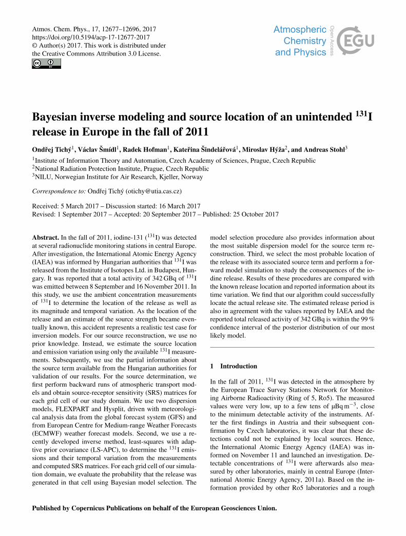
Figure 1. Measurements of 131I activity concentrations in ambientair made at the stations Budapest (a) and Praha (b) displayed viatheir daily mean concentration.

pattern search method (e.g., Zheng and Chen, 2010). Cer-vone and Franzese (2010) studied several error functions toidentify suitable measures and cost functions for optimiza-tions and Kovalets et al. (2011) used a fluid dynamics modelto build up a cost function which could be optimized. Thesemethods can be inconvenient due to problematic conver-gence and limited information on the uncertainty of the re-sults. Often, they provide only point estimates. Full posteriorprobability densities are provided using Bayesian techniqueswhere the prior model is typically constructed as an alterna-tive to the cost function in the optimization approach. Verypopular Bayesian inference techniques are random search al-gorithms such as Markov chain Monte Carlo (MCMC) meth-

ods. Examples for this type of approach are in Keats et al.(2007) and Senocak et al. (2008) where wind field parame-ters are also estimated along with the source term parameters,or Delle Monache et al. (2008), who studied the Algeciras ac-cidental release with the assumptions that the source geom-etry and release time are known. Another Bayesian formula-tion and inference using the maximum entropy principle wasproposed by Bocquet (2007) where the source term is mod-eled as three-dimensional (area plus time); hence, the sourceterm integrated over time and area is obtained. This approachwas tested for both cases of the European Tracer EXperiment(ETEX) (Krysta et al., 2008) and compared with the maxi-mum posterior estimator by Bocquet (2008) with further non-Gaussian assumptions such as positivity or boundedness. Re-cently, a likelihood-free approximate Bayesian computationmethod for the localization of a biochemical source was pro-posed by Ristic et al. (2015) where multiple dispersion mod-els can be used and even weighted using Bayesian model se-lection. An extensive review of the source term estimationand location is available in Hutchinson et al. (2017).

Recently, a Bayesian inverse method called least-squaresmethod with adaptive prior covariance (LS-APC) was pro-posed (Tichý et al., 2016) using the variational Bayes (VB)approximation. The method was validated on the basis ofthe ETEX experiment and it was shown that the dependencyon manual selection of model parameters is lower than inthe case of its predecessors. The key advantage of the VBapproach is its fast evaluation, which makes it suitable forcalculation of many possible source locations. However, themethod is known to underestimate uncertainty; therefore, wewill also use a more accurate approximation of the posteriordistribution based on the Gibbs sampler (GS) (Ulrych andŠmídl, 2017).

www.atmos-chem-phys.net/17/12677/2017/ Atmos. Chem. Phys., 17, 12677–12696, 2017

http://www.osski.hu

http://www.sujb.cz/monras/aplikace/monras_en.html


In this paper, we use the LS-APC method for inversionfor the case of the iodine release in Hungary in 2011. More-over, we derive the variational Bayesian model selection forthe LS-APC model. Using this methodology, we can com-pare the reliability of each SRS matrix from the selectedspatial domain at a reasonable computational cost. The samemethodology can be used to quantify uncertainty in the eval-uation of the SRS matrix. Specifically, if several possiblevariants of the SRS matrix computation are available, theBayesian model selection can evaluate their posterior prob-ability, providing an objective guideline for selection of themost likely dispersion model or weather data. In this study,we evaluate the probability of the SRS matrices obtainedusing backward runs of the dispersion models FLEXPART(Stohl et al., 2005) and Hysplit (Draxler and Hess, 1997),which were based on meteorological input data from GFSmeteorological fields with resolution of 0.5◦× 0.5◦ in thecase of FLEXPART and from GFS meteorological fields withresolutions of 0.5◦× 0.5◦ and 1◦× 1◦ and ECMWF meteo-rological fields with a resolution of 0.5◦× 0.5◦ in the caseof HYSPLIT. We identify the most probable release locationand derive the corresponding estimated source term. With alow number of selected locations, we run a more expensiveapproximation of the model based on Gibbs sampling whichis more computationally demanding. Using this source infor-mation, we perform a forward run and produce a 131I dosemap for Europe that can be used for impact assessment.

2 Measurement data

Iodine can exist in the atmosphere both as a gas and in theaerosol phase. Measurements of particulate phase 131I weremade at several stations of the Ro5 network, which is an in-formal information group established in 1983 for the purposeof rapidly exchanging data on occasional enhanced concen-trations of man-made radionuclides at trace levels. In total,117 131I measurements from 11 different sampling sites incentral Europe (see details in Table 1) obtained from Septem-ber to November 2011 were used in this study. As an exam-ple, measurements for the whole period from the Budapestand Praha stations are displayed in Fig. 1.

Atmospheric aerosol sampling was performed using var-ious types of high-volume samplers with flow rates rangingfrom 150 to 900 m3 h−1. In these devices, the air is filteredthrough glass-fiber or polypropylene filters, which capturethe radioactive aerosol with a high efficiency. As the labo-ratories operate under their own monitoring plans, samplingintervals differ both in length and starting day. In general,filters are changed every 3–7 days under normal conditions.Only in case of an emergency situation, the sampling periodwould be shortened.

After the sampling completion and decay of short-livedradon decay products, the filters are measured without ad-ditional chemical preparation in laboratories equipped with

a high-resolution gamma ray spectrometer. Since 131I emits364 keV photons with an intensity of 81 %, it allows a rea-sonably sensitive determination by a high-purity germanium(HPGe) spectrometer. In such a measurement arrangement,it is possible to achieve detection limits of several µBq m−3

but at the cost of a rather poor time resolution. Consideringthe 8.02 day half-life of 131I, the resulting activity value hasto be decay corrected, which requires the assumption that theconcentration in the air was constant during sampling.

3 Inverse modeling

We follow the concept of linear modeling of the atmo-spheric dispersion using a SRS matrix (e.g., see Seibert,2001; Wotawa et al., 2003; Seibert and Frank, 2004). In thisapproach, an atmospheric transport model is used to pro-vide the linear relationship between sources and atmosphericconcentrations. By assuming a release xi from the releasesite at time i, we can calculate the concentration responseat a receptor yj at time j . Notice that the simulated con-centration response can be compared directly with measuredconcentrations at the receptor. The ratio mij = yj/xi definesthe source-receptor sensitivity. Collecting all possible releasetimes in vector x ∈Rn and all possible receptor responses atall measurement sites and times into vector y ∈Rp we obtaina linear model

y =Mx+ ε, (1)

where M ∈Rp×n is a SRS matrix and ε ∈Rp is an obser-vation error including both model and measurement errors,where the model error contained in matrix M is projectedonto the observation vector. This concept of SRS is quite uni-versal and can be applied with both Lagrangian and Euleriantransport models in both forward and backward runs (Seib-ert and Frank, 2004). However, the assumption of linearityis justified only for passive tracers and substances which donot undergo nonlinear chemical transformations – which islargely the case for iodine, which is thought to have mainlylinear removal processes (radioactive decay and wet and drydeposition to the surface).

An estimate of the unknown vector x can be obtainedusing minimization of the model error (Eq. 1). However, aBayesian approach provides more informative results sinceit evaluates the full posterior density of the unknown. Thehigh computational cost of conventional Monte Carlo eval-uation methods can be avoided by using an approximationtechnique known as variational Bayes. This has been ana-lyzed in detail by Tichý et al. (2016), where a computation-ally efficient algorithm was presented. One of the key advan-tages is that all parameters of the regularization are estimatedtogether with the source term. In this paper, we provide anapproximate formula for the evaluation of the marginal like-lihood of the model, which is essential for Bayesian modelcomparison (Bernardo and Smith, 2009). In effect, this tech-



nique allows us to compare the likelihood of different ma-trices M which could describe atmospheric dispersion fromdifferent possible source locations or could originate fromdifferent atmospheric dispersion models.

Before reviewing the full probabilistic model, we wouldlike to illustrate its relation to the conventional cost optimiza-tion. Consider the quadratic norm of the residues of Eq. (1)

J = ω−20 (Mx− y)T (Mx− y) , (2)

with selected parameter ω0. The estimate 〈x〉 can be obtainedby minimizing the cost J (Eq. 2) plus additional regular-ization terms. In probabilistic interpretation, minimization ofEq. (2) is equivalent to maximization of the likelihood func-tion

p(y|x)=N(Mx,ω−1

0 Ip

)∝ exp

(−

12ω0(Mx− y)T (Mx− y)

), (3)

where N (µ,6) denotes a multivariate Gaussian distributionwith meanµ and covariance matrix 6, Ip is the p×p identitymatrix, and symbol ∝ denotes equality up to the normalizingconstant. In this case, 6 = ω−1

0 Ip and ω0 is known as theprecision parameter. The normalization constant is irrelevantfor maximization. However, it will become important for es-timating the precision parameter ω0. Due to the requirementof normalization, the Bayesian method allows us to estimateparameters of the prior distributions (which define the regu-larization terms in the cost formulation). To distinguish be-tween selected and estimated parameters, we denote all pres-elected parameters with subscript 0 and estimated model pa-rameters without the subscript.

After reviewing the selected Bayesian inverse method, wewill derive a lower bound on its marginal likelihood whichwill be used for selection of the most suitable model struc-ture. Specifically, we will use this tool to select from multipleSRS matrices arising from different settings of the disper-sion model. Multiple SRS matrices may arise, for examplewhen multiple atmospheric transport models are available,when varying model parameters, when multiple meteorolog-ical input data are available, or when SRS matrices are com-puted for each potential release site. The marginal likelihoodmeasure is able to select the most suitable model, with nat-ural penalization for complex models due to the principle ofmarginalization. Thus, the influence of the estimated tuningparameters (hyper-parameters of the prior) is minimized.

3.1 Review of model LS-APC

The probabilistic model of Tichý et al. (2016) is briefly re-viewed in this section. The likelihood function is consideredto be Gaussian (Eq. 3) with standard deviation ω being con-sidered as unknown. Thus, we need to select its prior distri-bution. We select the gamma distribution due to its conjugacywith Gaussian likelihood (Tipping and Bishop, 1999):

p(y|x,ω)=N(Mx,ω−1Ip

), (4)

p(ω)= G (ϑ0,ρ0) , (5)

where ϑ0,ρ0 are chosen constants. These constants areneeded for numerical stability; however, they are set as lowas possible such as to 10−10 to provide a non-informativeprior.

The prior distribution of the source term x is designed toencourage three properties: (i) non-negativeness of all ele-ments of x, (ii) sparsity, i.e., the element is zero unless thereis sufficient information on the opposite, and (iii) smooth-ness, i.e., that rapid changes in the temporal profile are pos-sible but not frequent. These properties are encoded into ahierarchical prior model

p(xj+1|xj , lj ,υj )= tN(−ljxj ,υ

−1j+1, [0,∞]

),

for j = 1, . . .,n− 1, (6)p(υj )= G (α0,β0) , for j = 1, . . .,n, (7)

p(lj |ψj )=N(−1,ψ−1

j

), for j = 1, . . .,n− 1, (8)

p(ψj )= G (ζ0,η0) , for j = 1, . . .,n− 1, (9)

where tN (µ,σ, [a,b]) denotes the truncated Gaussian dis-tribution on support [a,b], lj is a parameter modeling thesmoothness, i.e., the relation between neighboring elementsof the source term, and υj is its precision parameter. The

prior for element x1 is p(x1|υ1)= tN(

0,υ−11 , [0,∞]

). The

prior has constants α0,β0,ζ0,η0 that need to be selected.Good performance of the prior was reported with a non-informative choice of α0,β0, e.g., 10−10. The prior constantsζ0 and η0 are selected as 10−2 to favor a smooth solution, seediscussion in Tichý et al. (2016).

3.2 Model uncertainty

The original LS-APC model (Eqs. 4–9) assumes uncertaintyonly in the source term x and its hyper-parameters. How-ever, in real scenarios, the uncertainty is also present in theSRS matrix due to inaccurate meteorological data and/or in-accurate parameters of the dispersion model. Exact mod-eling of these uncertainties is too complex; therefore, weuse an approximation using discrete variables. Specifically,we assume that we have a finite set of SRS matrices, M={M1,M2, . . .,Mr} obtained by different versions of the dis-persion models and/or different meteorological data. Uncer-tainty in the SRS matrix and the potential bias of the results isthus reduced by estimating the probability that the data weregenerated by each of the tested SRS matrices. The result isthus a rational way to select the most likely dispersion modeland meteorology for a particular data set.



3.3 LS-APC model inference

The LS-APC model is a hierarchical Bayesian model de-signed to estimate its hyper-parameters from the data. Fora given model (SRS matrix)M , the task of the inference is touse the Bayes rule to find the posterior distribution

p(x|y,M)=p(y,x|M)

p(y|M), (10)

in which all nuisance parameters (i.e., ω,υ, l,ψ) have beenmarginalized (integrated out). The denominator of Eq. (10)is known as marginal likelihood and it is essential in evalua-tion of the probability of the model represented by the SRSmatrix from the set M= {M1, . . .,Mr}. The probability thatthe observed data were generated from the kth model, Mk ,k = 1, . . ., r can be formally obtained from the Bayes rule

p(M =Mk|y)∝ p(M =Mk)p(y|Mk). (11)

Here, symbol ∝ denotes equality up to a multiplicative con-stant, and p(M =Mk) denotes prior probability of the kthmodel. In our case we assume that all models have equalprior probability. Evaluation of Eqs. (10) and (11) is in-tractable and will be approximated by the variational Bayesand Gibbs sampling methods.

3.3.1 Variational Bayes inference

Under the VB approximation (Šmídl and Quinn, 2006), theposterior distributions are found in the same form as theirpriors (Eqs. 6–9) and their moments are determined by aniterative algorithm which is available in Matlab code as asupplement of Tichý et al. (2016). However, the value ofthe marginal likelihood p(y|M) is not available analyticallyand no approximation was presented in Tichý et al. (2016).The method will be referred to here as the LS-APC-VB al-gorithm.

Approximation of the marginal likelihood (Eq. 11) usingvariational Bayes methodology is computed as

p(M =Mk |y)∝ p(M =Mk)exp(LMk

), k = 1, . . ., r, (12)

whereLMkis a variational lower bound on p(y|Mk) (Bishop,

2006) given as

LMk=

∫p(x,ϒ,L,ψ,ω|Mk)p (Mk)

lnp(y,x,ϒ,L,ψ,ω,Mk)

p(x,ϒ,L,ψ,ω|Mk)p (Mk)dxdϒdLdψdω, (13)

where x,ϒ,L,ψ = [ψ1, . . .,ψn−1],ω are variables of theLS-APC model driven with the SRS matrix Mk (variables ϒandL are matrices defined in the Supplement). Equation (13)can be seen as a term composed of expected values (denotedas E[] with respect to distribution of the variable in its argu-ment) so that

LMk= E

[lnp(y,x,ϒ,L,ψ,ω,Mk)

]−E

[ln p(ω)

]−E

[ln p(x)

]−E

[ln p(ϒ)

]−E

[ln p(L)

]−E

[ln p(ψ)

], (14)

where p(y,x,ϒ,L,ψ,ω,Mk) is the joint distribution oflikelihood (Eq. 4) and prior probability distributions (Eq. 6–9), and p() are posterior probability distributions. Theseterms are given in the Supplement.

3.3.2 Gibbs sampling inference

An alternative approximation of the posterior (Eq. 10) is ob-tained using Gibbs sampling (GS). The method is closely re-lated to the VB method (Ormerod and Wand, 2010) using thesame forms of posterior with different interpretation. Whilethe variational Bayes approximation is looking for a goodfit of parametric form, the Gibbs sampling generates samplesfrom the conditional distribution and approximates the poste-rior by an empirical distribution on these samples. It has beenapplied to the LS-APC model by Ulrych and Šmídl (2017).In practical terms, the GS yields a more accurate approxi-mation, however, at the cost of a much higher computationalburden. While the VB method converges in fewer than 100 it-erations, the GS method needs about 1 000 000 samples toobtain a reliable estimate (one sample takes roughly the sameCPU time as one iteration of VB). However, the main advan-tage is that the GS method converges to the true posterior,while the VB method may converge to a local approxima-tion. The method will be referred to here as the LS-APC-GSalgorithm.

4 Atmospheric transport modeling

The SRS matrices in this work were computed using back-ward runs of two alternative models, namely HYSPLIT(Draxler and Hess, 1997) and FLEXPART (Stohl et al.,2005). As the domain of interest we chose the region span-ning from 5◦ E to 30◦ E in longitude and from 40◦ N to 65◦ Nin latitude covering most of Europe and parts of the Mediter-ranean Sea. Horizontally, the domain was discretized into2500 grid cells with resolution 0.5◦× 0.5◦, which approxi-mately corresponds to 45 km× 55 km at the latitude of Bu-dapest. Vertically, there is no discretization of the domainand sensitivities are calculated for a layer 0–300 m aboveground, which allows for both ground and somewhat elevatedreleases (e.g., through the stack of the isotope production fa-cility). Mixing heights are often higher than 300 m, in whichcase the result is not very sensitive to the choice of the depthof this layer. Temporal resolution of the source was set to 1day and we assume that the release occurred during a 91-daytime window starting on 1 September 2011.

As a result, the domain was discretized into227500 spatio-temporal sources for which their possi-ble contributions to all samples must be calculated. Since the



40◦ N

45◦ N

50◦ N

55◦ N

60◦ N

65◦ N

5◦ E 10◦ E 15◦ E 20◦ E 25 ◦ E 30 ◦ E

A

BCD

EF

GH

I

J

K

Source location - LS-APC-VB with Flexpart-GFS-0.5

A - BudapestB - PrahaC - RetzD - Alt-PrerauE - Usti nad LabemF - Ostrava

G - Ceske BudejoviceH - SanokI - GdyniaJ - KatowiceK - Zielona GoraIoI Budapest

165 180 195 210 225 240 255

40◦ N

45◦ N

50◦ N

55◦ N

60◦ N

65◦ N

5◦ E 10◦ E 15◦ E 20◦ E 25◦ E 30◦ E

A

BCD

EF

GH

I

J

K

Source location - LS-APC-VB with Hysplit-GFS-0.5



175 200 225 250 275 300 325 350 375

40◦ N

45◦ N

50◦ N

55◦ N

60◦ N

65◦ N

5◦ E 10◦ E 15◦ E 20◦ E 25◦ E 30◦ E

A

BCD

EF

GH

I

J

K




165 180 195 210 225 240 255 270

40◦ N

45◦ N

50◦ N

55◦ N

60◦ N

65◦ N

5◦ E 10◦ E 15◦ E 20◦ E 25◦ E 30◦ E

A

BCD

EF

GH

I

J

K

Source location - LS-APC-VB with Hysplit-ECMWF-0.5



165 180 195 210 225 240 255 270

1

(a) (b)

(c) (d)

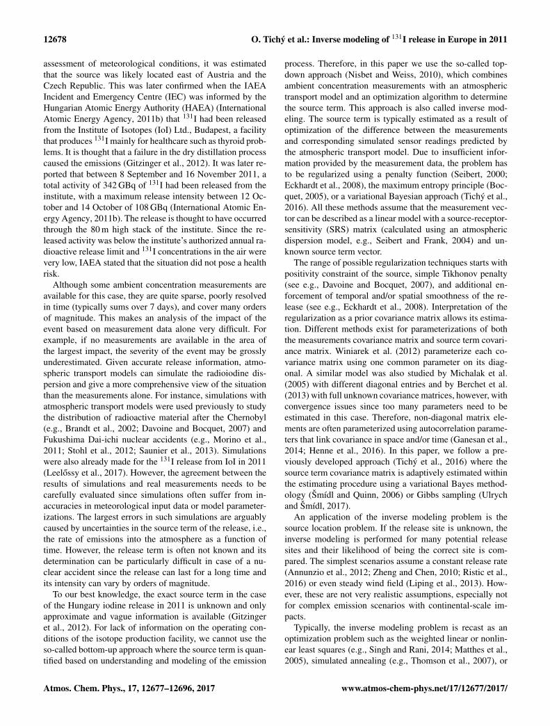
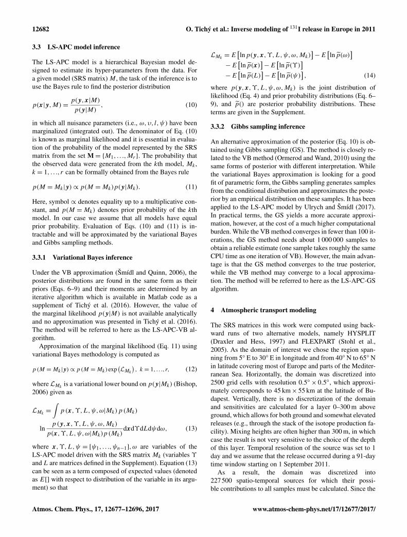
Figure 2. Source location via marginal log-likelihood where the observed data are explained by a release from a grid cell using the LS-APC-VB algorithm for all four tested combinations of dispersion model and meteorological data: Flexpart-GFS-0.5 (a), Hysplit-GFS-0.5(b), Hysplit-GFS-1.0 (c), and Hysplit-ECMWF-0.5 (d). The measuring sites (a list is given in Table 1) are displayed using green circles whilethe location of the Institute of Isotopes (IoI) Ltd. is displayed using a red cross.

number of candidate sources is much higher than the numberof measurement samples, the SRS matrices were obtainedusing backward runs of the model from the sampling sites.One backward run was started exactly at the point locationof each measurement site and for each period correspondingexactly to a measurement sample. Each of the 117 backwardruns corresponding to the 117 available measurementsprovided a SRS matrix of a particular sample to all candidatespatio-temporal sources in our domain. Since we a prioriassume that the release occurred from a point source (i.e., asingle horizontal grid cell), we can calculate SRS fields froma single grid cell at once, which allows parallelization of thecomputations. We end up with 2500 SRS matrices (one for

each of the 50× 50 model grid cells) of dimension 117× 91from each transport model.

Radioiodine can be present in the atmosphere as molecularI2, as organic iodide, or as iodide salts. The former two areexpected to exist as gases, while the latter is an aerosol. Inwhich form iodine is released to the environment from a nu-clear facility depends on its operating conditions (Simondi-Teisseire et al., 2013). Iodine chemistry in the atmosphere iscomplex and can involve, for instance, chemical transforma-tion of the different compounds and particle formation (Saiz-Lopez et al., 2012). As every compound has its own scav-enging efficiency, both with respect to dry and wet deposi-tion, accurate modeling of iodine is complicated. We chose asimple approach for our modeling, namely assuming that all



released 131I was in particulate form, which most probablydominated the release. This is also justified by the fact thatall of the measurements we have available were made forparticulate iodine only. Consequently, in both models, 131Iwas simulated as an aerosol. In FLEXPART, parameters ofthe dry and wet deposition were set to default values for 131Iin the FLEXPART 9.2 species library and radioactive decay(ingrowth during backward runs) was calculated on the fly. InHYSPLIT, parameters of the dry and wet deposition were setto default values for aerosol 131I, except for predefined drydeposition velocity which was set to 5.7 mm s−1 accordingto measurements of Takeyasu and Sumiya (2014). HYSPLITcalculated with an 131I radioactive decay half-life of 8 days.Our inverse modeling would thus not capture gaseous 131I,which may have been co-emitted, except indirectly if someof this gaseous 131I condensed on or formed particles thatwere subsequently measured. Our results are thus lower es-timates of the total 131I release, but the bias is probably notvery large.

4.1 FLEXPART

FLEXPART (FLEXible PARTicle dispersion model) is a sci-entific model used worldwide by many research groups andalso operationally, e.g., at the Comprehensive Nuclear-Test-Ban Treaty Organization for routine atmospheric backtrack-ing (Kalinowski et al., 2008). In this work we used version9.2 (Stohl et al., 2005). Runs were forced with GFS meteo-rological fields with 0.5◦×0.5◦ horizontal resolution and 26vertical layers and temporal resolution of 3 h. During all cal-culations, the convection scheme was enabled in FLEXPARTfor more realistic simulation of vertical air mass fluxes whenconvective conditions are encountered (Forster et al., 2007).

Simulations in FLEXPART can be carried out on two dif-ferent output grids in a single run. The so-called mothergrid is usually a global grid with coarser resolution, whereasthe nested grid is a smaller subdomain with higher horizon-tal resolution (vertical resolution must be the same for bothgrids). Our domain of interest was a nested output grid withhorizontal resolution 0.5◦× 0.5◦, whereas the global gridwith resolution 1◦× 1◦ was the mother grid. The simula-tions accounted for dry deposition using a resistance method.Wet scavenging was accounted for with a scheme that distin-guishes between in-cloud and below-cloud scavenging.

4.2 HYSPLIT

The HYSPLIT (HYbrid Single-Particle Lagrangian Inte-grated Trajectory) model is a model widely used to simu-late atmospheric transport and dispersion on various levelsof complexity. Its applications range from simple estimationof forward and backward trajectories of air parcels, to ad-vanced modeling of transport, dispersion and deposition ofair masses on large domains. HYSPLIT adopts a hybrid ap-proach combining the Lagrangian (moving frame of refer-

ence for diffusion and advection) and Eulerian (fixed modelgrid for calculation of air concentration) model methodolo-gies. In this study we applied HYSPLIT model version 4(Draxler and Hess, 1997, 1998; Draxler and Rolph, 2003;Stein et al., 2015).

The model was forced with GFS analyses with horizon-tal resolution of 0.5◦× 0.5◦, 26 vertical layers and 6-hourlytemporal resolution. The model domain covered most of theEuropean continent. The HYSPLIT model was also forcedwith GFS analyses with a horizontal resolution of 1◦× 1◦,26 vertical layers, and 6-hourly temporal resolution to testthe sensitivity of the source re-construction to meteorolog-ical input data resolution. This data set was only availablein a format suitable for HYSPLIT but not for FLEXPART.The resolution of the output grid was the same as used withFLEXPART, i.e., 0.5◦×0.5◦. The HYSPLIT model was alsoforced with the ERA-Interim reanalysis (Dee et al., 2011)data from the European Centre for Medium-range WeatherForecast (ECMWF) with 0.5◦× 0.5◦ horizontal resolution,36 vertical layers, and temporal resolution of 6 hours.

5 Results and discussion

In this section, we apply the Bayesian inverse modelingmethod introduced in Sect. 3 to iodine measurements de-scribed in Sect. 2 and computed SRS matrices from Sect.4 for all four cases: (i) FLEXPART driven with the GFSanalyses with the resolution 0.5◦× 0.5◦ (Flexpart-GFS-0.5),(ii) HYSPLIT driven with the GFS analyses with the reso-lution 0.5◦× 0.5◦ (Hysplit-GFS-0.5), (iii) HYSPLIT drivenwith the GFS analyses with the resolution 1◦× 1◦ (Hysplit-GFS-1.0), and (iv) HYSPLIT driven with the ECMWF analy-ses with resolution 0.5◦×0.5◦ (Hysplit-ECMWF-0.5). First,we will study the problem of source location and after thatwe will discuss the source term as a function of time for themost probable source location.

5.1 Source location

The LS-APC-VB inversion method, described in Sect. 3, wasapplied to each grid cell in our domain (notice that eachgrid cell is a candidate source location) for each combina-tion of atmospheric transport model and meteorological in-put data. Hence, our set of SRS matrices is defined as M={M(i,j,m); i = 1, . . .,50, j = 1,50, m= 1, . . .,4}, where i,jare coordinates of the (i,j)th tile on the map and m isthe number of specific combination of atmospheric transportmodel driven with meteorological input data. For each SRSmatrix from the set M, the method also provides the varia-tional lower bound LM(i,j,m)

, Eq. (14), which correspond tothe probability that the release happened in grid cell (i,j)for the given atmospheric model. Note that no prior informa-tion on source location, p

(M(i,j,m) =M

)in Eq. (12), is used

which is equal to omitting of this term due to proportional



0

50

100

150

Est

imat

ed s

ourc

e te

rm (

GB

q)

LS−APC−VB with Flexpart−GFS−0.5

01/0915/09

30/0915/10

31/1015/11

30/11

1117 GBq, unc. bounds [963,1271] GBq

0

50

100

150

Est

imat

ed s

ourc

e te

rm (

GB

q)

LS−APC−VB with Hysplit−GFS−0.5

01/0915/09

30/0915/10

31/1015/11

30/11


0

10

20

30

40

50

Est

imat

ed s

ourc

e te

rm (

GB

q)


01/0915/09

30/0915/10

31/1015/11

30/11


0

10

20

30

40

50

Est

imat

ed s

ourc

e te

rm (

GB

q)

LS−APC−VB with Hysplit−ECMWF−0.5

01/0915/09

30/0915/10

31/1015/11

30/11


(a) (b)

(c) (d)

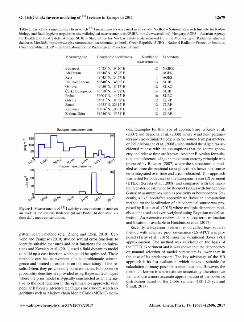
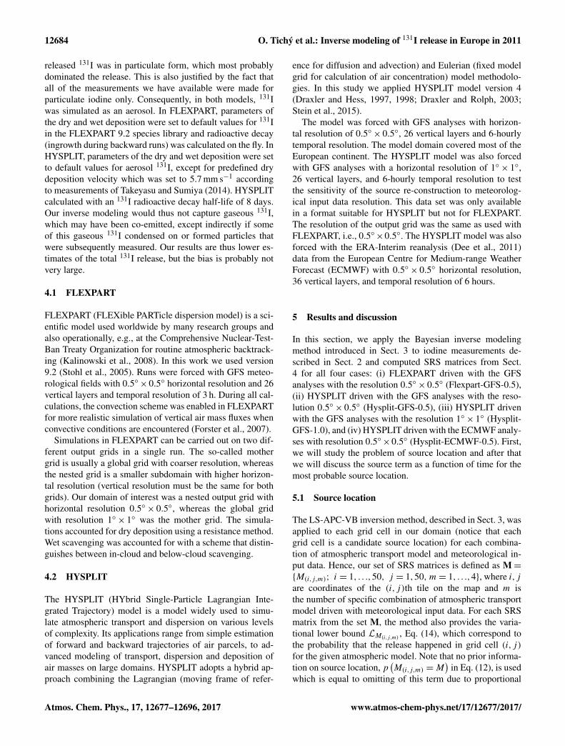
Figure 3. Estimated source terms at locations selected by the marginal likelihood method, shown in Fig. 2, using the LS-APC-VB algorithmfor all four tested combinations of dispersion models and meteorological data: Flexpart-GFS-0.5 (a), Hysplit-GFS-0.5 (b), Hysplit-GFS-1.0(c), and Hysplit-ECMWF-0.5 (d). The estimated source terms are accompanied by the 95 % uncertainty regions (gray filled regions). Theestimated activity for the whole period is reported inside each plot with its associated uncertainty bounds.

0 100 2000

50

100

150

200

y (µBq m )-3

M*x

(µB

q m

)

-3


0 100 2000

50

100

150

200

y (µBq m )-3

M*x

(µB

q m

)

-3


0 100 2000

50

100

150

200

y (µBq m )-3

M*x

(µB

q m

)

-3


0 100 2000

50

100

150

200

y (µBq m )-3

M*x

(µB

q m

)-3


(a) (b)

(c) (d)

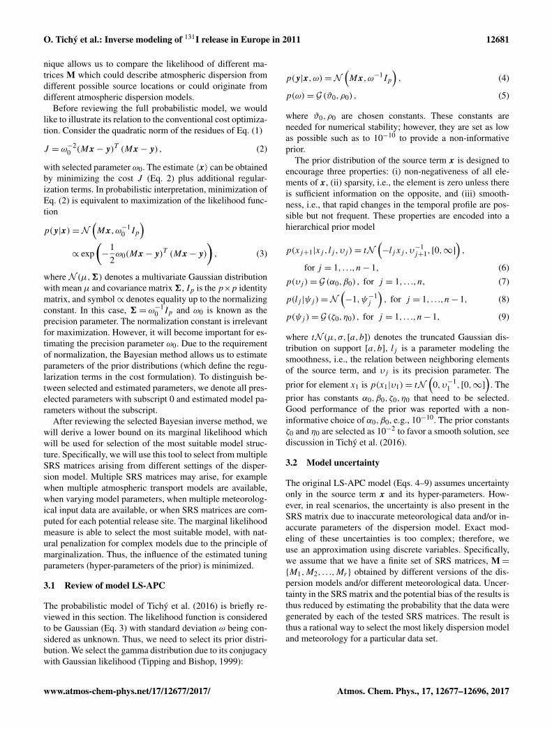
Figure 4. Scatter plots of the measurements y and the reconstructedsignal Mx using the LS-APC-VB algorithm with Flexpart-GFS-0.5 (a), Hysplit-GFS-0.5 (b), Hysplit-GFS-1.0 (c), and Hysplit-ECMWF-0.5 (d). The reconstructions are given for the estimatedsource locations, shown in Fig. 2, and the mean values of the esti-mated source terms, shown with blue lines in Fig. 3.

equality in the equation. The results are presented in Fig. 2for Flexpart-GFS-0.5 (a), Hysplit-GFS-0.5 (b), Hysplit-GFS-1.0 (c), and Hysplit-ECMWF-0.5 (d).

In all four cases, the source location mechanism of theLS-APC-VB method works very well and the maxima of thevariational lower boundLM(i,j,m)

are close to the true locationof the IoI. Note that the exact location of the IoI is 18.96◦ Eand 47.49◦ N, which is in the corner of a grid cell in the caseof 0.5◦ resolution; hence, we assume all results close to thispoint to be very good. In the case of Flexpart-GFS-0.5, theestimated release site is on the edge and southeast of the ac-tual release site. For both Hysplit-GFS cases with resolutionsof 1.0 and 0.5, respectively, the release site is found on theedge and northwest of the actual release site, while when us-ing Hysplit-ECMWF-0.5, the estimated release site is north-east and on the edge of the actual release site. In summary,the release site was well estimated using all atmosphericmodels in tandem with the LS-APC-VB algorithm. In all fourcases, some uncertainty remains especially to the south of theIoI where no measured data are available while in the north,the uncertainty is very small because the relatively densemeasurement network there effectively excludes the possi-bility of a source in this region. This is a typical problem ofinverse methods when the geometry of the sampling networkis sub-optimal and the source location is not surrounded bystations. This situation is similar to tomographic reconstruc-tions, e.g., in medical applications, where the reconstructionquality is always best when measurements can be taken allaround the phantom. Nonetheless, we conclude that the LS-



0

10

20

30

40

50

Est

imat

ed s

ourc

e te

rm (

GB

q)

LS−APC−GS with Flexpart−GFS−0.5

01/0915/09

30/0915/10

31/1015/11

30/11


0

10

20

30

40

50

Est

imat

ed s

ourc

e te

rm (

GB

q)

LS−APC−GS with Hysplit−GFS−0.5

01/0915/09

30/0915/10

31/1015/11

30/11


0

10

20

30

40

50

Est

imat

ed s

ourc

e te

rm (

GB

q)


01/0915/09

30/0915/10

31/1015/11

30/11


0

10

20

30

40

50

Est

imat

ed s

ourc

e te

rm (

GB

q)

LS−APC−GS with Hysplit−ECMWF−0.5

01/0915/09

30/0915/10

31/1015/11

30/11


(a) (b)

(c) (d)

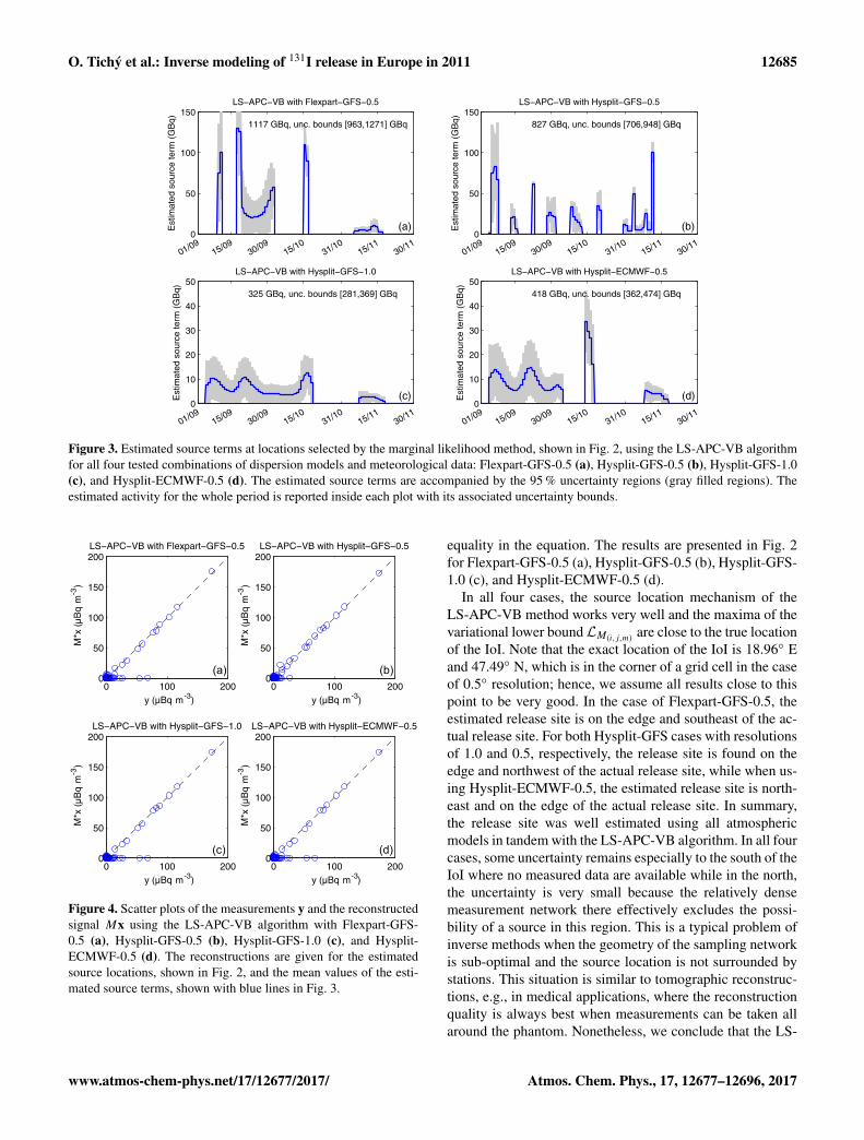
Figure 5. Estimated source terms at locations selected by the marginal likelihood method, shown in Fig. 2, using the LS-APC-GS algorithmfor all four tested combinations of dispersion models and meteorological data: Flexpart-GFS-0.5 (a), Hysplit-GFS-0.5 (b), Hysplit-GFS-1.0 (c), and Hysplit-ECMWF-0.5 (d). The estimated source terms are accompanied by the 95 % uncertainty regions (gray filled regions). Theestimated activity for the whole period is reported inside each plot with its associated uncertainty bounds.

40◦ N

45◦ N

50◦ N

55◦ N

60◦ N

65◦ N

5◦ E 10◦ E 15◦ E 20◦ E 25◦ E 30◦ E

A

BCD

EF

GH

I

J

K

Hys-GFS-0.5 20110914 00:00, concentration [μBq m-3]



10 5 10 4 10 3 10 2 10 1 10 0 10 1 10 2 10 3

40◦ N

45◦ N

50◦ N

55◦ N

60◦ N

65◦ N

5◦ E 10◦ E 15◦ E 20◦ E 25◦ E 30◦ E

A

BCD

EF

GH

I

J

K




10 5 10 4 10 3 10 2 10 1 10 0 10 1 10 2 10 3

40◦ N

45◦ N

50◦ N

55◦ N

60◦ N

65◦ N

5◦ E 10◦ E 15◦ E 20◦ E 25◦ E 30◦ E

A

BCD

EF

GH

I

J

K




10 5 10 4 10 3 10 2 10 1 10 0 10 1 10 2 10 3

1

(a) (b) (c)

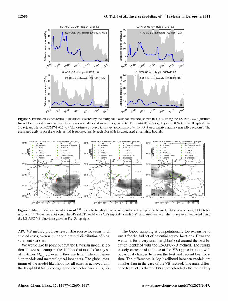
Figure 6. Maps of daily concentrations of 131I for selected days (dates are reported at the top of each panel, 14 September in a, 14 Octoberin b, and 14 November in c) using the HYSPLIT model with GFS input data with 0.5◦ resolution and with the source term computed usingthe LS-APC-VB algorithm given in Fig. 3, top right.

APC-VB method provides reasonable source locations in allstudied cases, even with the sub-optimal distribution of mea-surement stations.

We would like to point out that the Bayesian model selec-tion allows us to compare the likelihood of models for any setof matrices M(i,j,m), even if they are from different disper-sion models and meteorological input data. The global max-imum of the model likelihood for all cases is achieved withthe Hysplit-GFS-0.5 configuration (see color bars in Fig. 2).

The Gibbs sampling is computationally too expensive torun it for the full set of potential source locations. However,we ran it for a very small neighborhood around the best lo-cation identified with the LS-APC-VB method. The resultsclosely correspond to those of the VB approximation, withoccasional changes between the best and second best loca-tion. The differences in log-likelihood between models aresmaller than in the case of the VB method. The main differ-ence from VB is that the GS approach selects the most likely



40◦ N

45◦ N

50◦ N

55◦ N

60◦ N

65◦ N

5◦ E 10◦ E 15◦ E 20◦ E 25◦ E 30◦ E

A

BCD

EF

GH

I

J

K

Forward run of Hysplit-GFS-0.5, total dose [mSv]



10 − 7 10 − 6 10 − 5 10 − 4 10 − 3

40◦ N

45◦ N

50◦ N

55◦ N

60◦ N

65◦ N

5◦ E 10◦ E 15◦ E 20◦ E 25◦ E 30◦ E

A

BCD

EF

GH

I

J

K

Forward run of Hysplit-GFS-1.0, total dose [mSv]



10 − 7 10 − 6 10 − 5 10 − 4 10 − 3

1

(a) (b)

Figure 7. 131I total dose for the whole 3-month studied interval. (a) Simulation using the HYSPLIT model with GFS input data with 0.5◦

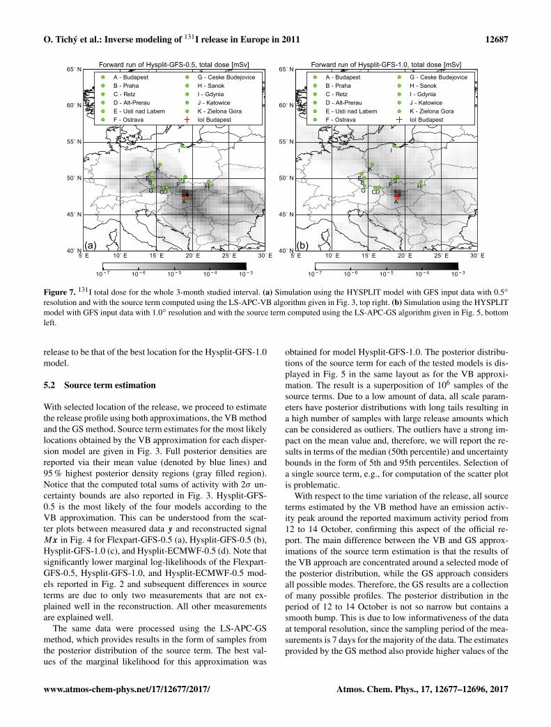
resolution and with the source term computed using the LS-APC-VB algorithm given in Fig. 3, top right. (b) Simulation using the HYSPLITmodel with GFS input data with 1.0◦ resolution and with the source term computed using the LS-APC-GS algorithm given in Fig. 5, bottomleft.

release to be that of the best location for the Hysplit-GFS-1.0model.

5.2 Source term estimation

With selected location of the release, we proceed to estimatethe release profile using both approximations, the VB methodand the GS method. Source term estimates for the most likelylocations obtained by the VB approximation for each disper-sion model are given in Fig. 3. Full posterior densities arereported via their mean value (denoted by blue lines) and95 % highest posterior density regions (gray filled region).Notice that the computed total sums of activity with 2σ un-certainty bounds are also reported in Fig. 3. Hysplit-GFS-0.5 is the most likely of the four models according to theVB approximation. This can be understood from the scat-ter plots between measured data y and reconstructed signalMx in Fig. 4 for Flexpart-GFS-0.5 (a), Hysplit-GFS-0.5 (b),Hysplit-GFS-1.0 (c), and Hysplit-ECMWF-0.5 (d). Note thatsignificantly lower marginal log-likelihoods of the Flexpart-GFS-0.5, Hysplit-GFS-1.0, and Hysplit-ECMWF-0.5 mod-els reported in Fig. 2 and subsequent differences in sourceterms are due to only two measurements that are not ex-plained well in the reconstruction. All other measurementsare explained well.

The same data were processed using the LS-APC-GSmethod, which provides results in the form of samples fromthe posterior distribution of the source term. The best val-ues of the marginal likelihood for this approximation was

obtained for model Hysplit-GFS-1.0. The posterior distribu-tions of the source term for each of the tested models is dis-played in Fig. 5 in the same layout as for the VB approxi-mation. The result is a superposition of 106 samples of thesource terms. Due to a low amount of data, all scale param-eters have posterior distributions with long tails resulting ina high number of samples with large release amounts whichcan be considered as outliers. The outliers have a strong im-pact on the mean value and, therefore, we will report the re-sults in terms of the median (50th percentile) and uncertaintybounds in the form of 5th and 95th percentiles. Selection ofa single source term, e.g., for computation of the scatter plotis problematic.

With respect to the time variation of the release, all sourceterms estimated by the VB method have an emission activ-ity peak around the reported maximum activity period from12 to 14 October, confirming this aspect of the official re-port. The main difference between the VB and GS approx-imations of the source term estimation is that the results ofthe VB approach are concentrated around a selected mode ofthe posterior distribution, while the GS approach considersall possible modes. Therefore, the GS results are a collectionof many possible profiles. The posterior distribution in theperiod of 12 to 14 October is not so narrow but contains asmooth bump. This is due to low informativeness of the dataat temporal resolution, since the sampling period of the mea-surements is 7 days for the majority of the data. The estimatesprovided by the GS method also provide higher values of the



40◦ N

45◦ N

50◦ N

55◦ N

60◦ N

65◦ N

5◦ E 10◦ E 15◦ E 20◦ E 25◦ E 30◦ E

A

BCD

EF

GH

I

J

K

Source location - LS-APC-VB with Flexpart-GFS-0.5



180 200 220 240 260 280 300

40◦ N

45◦ N

50◦ N

55◦ N

60◦ N

65◦ N

5◦ E 10◦ E 15◦ E 20◦ E 25◦ E 30◦ E

A

BCD

EF

GH

I

J

K




180 200 220 240 260 280 300 320

40◦ N

45◦ N

50◦ N

55◦ N

60◦ N

65◦ N

5◦ E 10◦ E 15◦ E 20◦ E 25◦ E 30◦ E

A

BCD

EF

GH

I

J

K




180 200 220 240 260 280 300 320

40◦ N

45◦ N

50◦ N

55◦ N

60◦ N

65◦ N

5◦ E 10◦ E 15◦ E 20◦ E 25◦ E 30◦ E

A

BCD

EF

GH

I

J

K

Source location - LS-APC-VB with Hysplit-ECMWF-0.5



180 200 220 240 260 280 300

(a) (b)

(c) (d)

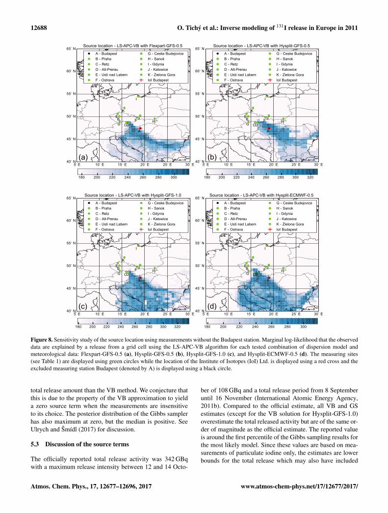
Figure 8. Sensitivity study of the source location using measurements without the Budapest station. Marginal log-likelihood that the observeddata are explained by a release from a grid cell using the LS-APC-VB algorithm for each tested combination of dispersion model andmeteorological data: Flexpart-GFS-0.5 (a), Hysplit-GFS-0.5 (b), Hysplit-GFS-1.0 (c), and Hysplit-ECMWF-0.5 (d). The measuring sites(see Table 1) are displayed using green circles while the location of the Institute of Isotopes (IoI) Ltd. is displayed using a red cross and theexcluded measuring station Budapest (denoted by A) is displayed using a black circle.

total release amount than the VB method. We conjecture thatthis is due to the property of the VB approximation to yielda zero source term when the measurements are insensitiveto its choice. The posterior distribution of the Gibbs samplerhas also maximum at zero, but the median is positive. SeeUlrych and Šmídl (2017) for discussion.

5.3 Discussion of the source terms

The officially reported total release activity was 342 GBqwith a maximum release intensity between 12 and 14 Octo-

ber of 108 GBq and a total release period from 8 Septemberuntil 16 November (International Atomic Energy Agency,2011b). Compared to the official estimate, all VB and GSestimates (except for the VB solution for Hysplit-GFS-1.0)overestimate the total released activity but are of the same or-der of magnitude as the official estimate. The reported valueis around the first percentile of the Gibbs sampling results forthe most likely model. Since these values are based on mea-surements of particulate iodine only, the estimates are lowerbounds for the total release which may also have included



radioiodine gas. Moreover, the results are subject to manyunmodeled uncertainties which are now discussed.

First, one has to consider uncertainty due to the long sam-pling period of the measurements, mostly 7 days. This maylead to a large uncertainty in estimated source terms since theinversion method tries to capture a source term with resolu-tion of one day from such a time-insensitive measurement.The second source of uncertainty is the relatively coarse dis-cretization of the studied domain and the proximity of theIoI facility and the measuring station Budapest (approxi-mately 10 km). Since concentration gradients cannot be re-solved within one grid cell, the inversion may try to com-pensate this by overestimation of the source term to fit theBudapest measurements. The third source of uncertainty ofthe source term is the selected atmospheric dispersion mod-els (and their parameterizations). For example, both atmo-spheric transport models may simulate too short a lifetime ofparticulate iodine. This, as for many other models, was foundfor Cs-137 attached to particles after the Fukushima Dai-ichiaccident (Kristiansen et al., 2016). The inversion would prob-ably try to compensate a too strong loss of mass by increas-ing the emitted amount. The fourth source of uncertainty isthe input data from meteorological reanalysis. As shown byLeelossy et al. (2017), the example meteorological situationon 4 November in 2011 in central Europe was very complexwith low-level inversion where the winds below the inver-sion level were significantly different than the winds above.Subsequently, if boundary layer heights were systematicallytoo high, simulated ground-level concentrations may be sys-tematically too low. This would be probably compensated bythe inversion with a too large emitted amount. In these andother complex situations, different models may provide verydifferent performances (Leelossy et al., 2017).

Given all these uncertainties and also the fact that in ourstudy different atmospheric transport models driven withdifferent meteorological reanalyses provide different sourceterms, one should be cautious in comparing the total esti-mated release with the reported release amount. An agree-ment of the total amount of released 131I within one orderof magnitude may be the maximum which can be expected.This is reflected by the large uncertainty ranges obtained withour method. A positive result is that the models selected bythe marginal likelihood provide results closer to the reportedvalues than the other models. Our model ensemble is toosmall to fully capture the uncertainty related to the choiceof the dispersion model or meteorological input data. Never-theless, our small ensemble shows that the results are quitesensitive to the choice of the model. Particularly noteworthyis the large difference between Hysplit-GFS-1.0 and Hysplit-GFS-0.5, since these use the same dispersion model and me-teorological input data, except for the resolution of the latter.

This high sensitivity is at least partly related to the smallnumber of available 131I measurements. The inversion maytake advantage of certain model features to fit the modelresults to the few measurements. Such “overfitting” by ex-

ploiting particular model characteristics is less likely to besuccessful for a larger measurement data set. Clearly, moremeasurements are needed for a more reliable source termestimation. Nevertheless, the estimated source terms are ofthe right order of magnitude and the estimated release peri-ods between early September and mid-November correspondwell with the reported probable release period of 8 Septem-ber to 16 November (International Atomic Energy Agency,2011b).

5.4 Forward modeling of the iodine release

Using the estimated source location and source term, we canperform a forward run of the model and study the simulatedconsequences of the accidental release. For this purpose, weidentify the most probable location of the release from allcases evaluated by the LS-APC-VB method (Fig. 2), whichis the location with center at 18.75◦ E and 47.75◦ N obtainedwith the Hysplit-GFS-0.5 configuration with log-likelihoodup to 340. Therefore, we perform a forward run with theHYSPLIT model and GFS input data with 0.5◦ resolutionwith the corresponding source term shown in the top rightpanel of Fig. 3. The forward model run was set up in thesame manner as the backward runs. The output concentra-tions presented in Fig. 6 are mean values in the layer betweenthe surface and 100 m above ground level. The results for themost likely location selected by the LS-APC-GS method areanalogous.

The computed concentrations of 131I are displayed inFig. 6 for selected days, which are 14 September (a), 14 Oc-tober (b), and 14 November (c). The first two maps illustratechallenges for inverse modeling, since the aerosol was trans-ported to areas where no measurement data are available,which corresponds well with reported measurements fromBudapest and Praha in Fig. 1 where no measured activity isreported in Praha for the first half of the studied period. Thisalso implies that the results may be very sensitive to the mea-surements from the station Budapest (denoted by the letter Ain Fig. 6), which is the only station influenced in this case.This sensitivity will be studied in the next section.

The cumulated gamma dose for the whole 3-month periodis computed for the most probable source terms computed us-ing LS-APC-VB and LS-APC-GS methods. The cumulatedgamma dose for the LS-APC-VB estimate is displayed inFig. 7a, for the Hysplit-GFS-0.5 model with the same set-tings as in the case of concentrations and for the LS-APC-GS estimate is displayed in Fig. 7b, for the Hysplit-GFS-1.0model. Results show that gamma dose amounts were largestin Hungary and Slovakia, while in the rest of Europe theywere about 2 orders of magnitude smaller. However, Fig. 7also shows that most of Europe was affected to some extentby the release. Notably, the simulation also shows that boththe concentrations and dose amounts were very low evenclose to the release site. The maximum dose from the 131Irelease during the studied 3-month period is approximately



0

100

200

300

400

500

600

Est

imat

ed s

ourc

e te

rm (

GB

q)


01/0915/09

30/0915/10

31/1015/11

30/11


0

50

100

150

Est

imat

ed s

ourc

e te

rm (

GB

q)


01/0915/09

30/0915/10

31/1015/11

30/11


0

50

100

150

Est

imat

ed s

ourc

e te

rm (

GB

q)


01/0915/09

30/0915/10

31/1015/11

30/11


0

50

100

150

Est

imat

ed s

ourc

e te

rm (

GB

q)


01/0915/09

30/0915/10

31/1015/11

30/11


(a) (b)

(c) (d)

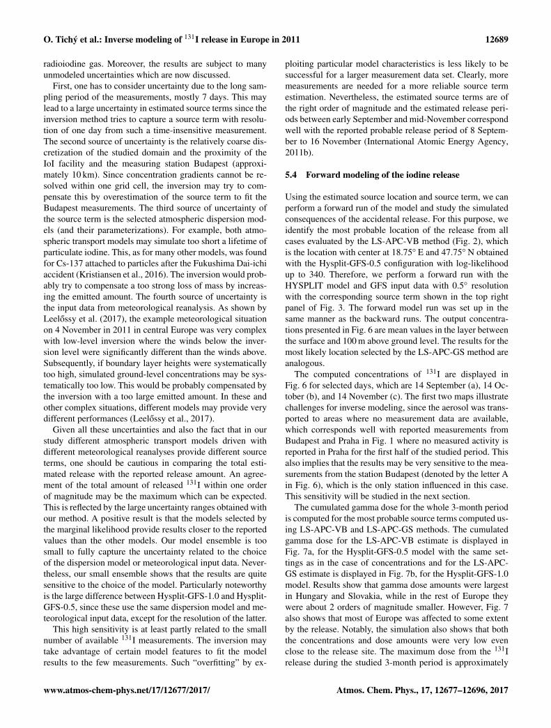
Figure 9. Estimated source terms at locations selected by the marginal likelihood method, shown in Fig. 8, with excluded measurementsfrom Budapest using the LS-APC-VB algorithm for all four tested combinations of dispersion models and meteorological data: Flexpart-GFS-0.5 (a), Hysplit-GFS-0.5 (b), Hysplit-GFS-1.0 (c), and Hysplit-ECMWF-0.5 (d). The estimated source terms are accompanied by the95 % uncertainty regions (gray filled regions). The estimated activity for the whole period is reported inside each plot with its associateduncertainty bounds.

0

50

100

150

Est

imat

ed s

ourc

e te

rm (

GB

q)

LS−APC−GS with Flexpart−GFS−0.5

01/0915/09

30/0915/10

31/1015/11

30/11


0

50

100

150

Est

imat

ed s

ourc

e te

rm (

GB

q)


01/0915/09

30/0915/10

31/1015/11

30/11


0

50

100

150

Est

imat

ed s

ourc

e te

rm (

GB

q)


01/0915/09

30/0915/10

31/1015/11

30/11


0

50

100

150

Est

imat

ed s

ourc

e te

rm (

GB

q)

LS−APC−GS with Hysplit−ECMWF−0.5

01/0915/09

30/0915/10

31/1015/11

30/11


(a) (b)

(c) (d)

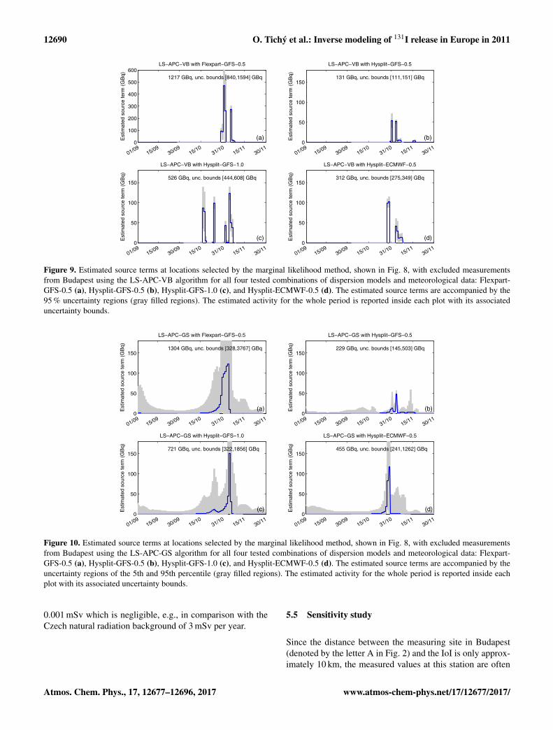
Figure 10. Estimated source terms at locations selected by the marginal likelihood method, shown in Fig. 8, with excluded measurementsfrom Budapest using the LS-APC-GS algorithm for all four tested combinations of dispersion models and meteorological data: Flexpart-GFS-0.5 (a), Hysplit-GFS-0.5 (b), Hysplit-GFS-1.0 (c), and Hysplit-ECMWF-0.5 (d). The estimated source terms are accompanied by theuncertainty regions of the 5th and 95th percentile (gray filled regions). The estimated activity for the whole period is reported inside eachplot with its associated uncertainty bounds.

0.001 mSv which is negligible, e.g., in comparison with theCzech natural radiation background of 3 mSv per year.

5.5 Sensitivity study

Since the distance between the measuring site in Budapest(denoted by the letter A in Fig. 2) and the IoI is only approx-imately 10 km, the measured values at this station are often



1 order of magnitude higher than those from the other sta-tions. Determining the source location and source strengthcould be thus dominated by the measurements from Bu-dapest. However, simulating the concentrations at such ashort distance is inaccurate since the meteorological inputdata are much coarser than the distance from the source to thestation, and also the SRS calculations are done on a coarsergrid. Thus, the errors of the source-location sensitivity canbe relatively large, which may influence the estimated sourceterm.

To test the sensitivity of the results to the values from theBudapest station, we run the source location excluding thosemeasurements. The results are given in Fig. 8. The data inthis case are much less informative hence the uncertainty insource location is much higher. Nevertheless, the maximumis mostly reached relatively close to the IoI facility. The max-ima for individual dispersion models are 17.75◦ E, 47.25◦ Nfor Flexpart-GFS-0.5; 18.75◦ E, 48.25◦ N for Hysplit-GFS-0.5; 19.25◦ E, 46.75◦ N for Hysplit-GFS-1.0; and 16.25◦ E,48.25◦ N for Hysplit-ECMWF-0.5; while the exact locationof the IoI is approximately 18.96◦ E, 47.49◦ N. Thus, even inthis poorly informative case, the location is identified withvery good accuracy. In all four cases, the uncertainty in-creased significantly to the south of the IoI where no mea-sured data are available.

Source term estimates done without using Budapest datafor the most likely locations for each dispersion model aregiven in Fig. 9. Full posterior densities are reported via theirmean value (denoted by blue lines) and 95 % highest poste-rior density regions (gray filled region). The source terms areaccompanied by the computed total sum of activity with 95 %uncertainty bounds. Overall, the total activities of estimatedFlexpart-GFS-0.5, Hysplit-GFS-1.0, and Hysplit-ECMWF-0.5 source terms are on the same level as in the previouscase where measurements from Budapest are included whilethe Hysplit-GFS-0.5 result is reduced approximately 6 times;however, note that the maximum of the log-likelihood isno longer reached by Hysplit-GFS-0.5 but by Hysplit-GFS-1.0 where the total activity of the source term is estimatedas 526 GBq with uncertainty bounds [444,608]GBq, whichis of the same order of magnitude as the reported amount342 GBq. Notice in particular that the reported peak relatedto the period 1 to 14 October is well captured by the LS-APC-VB algorithm with Hysplit-GFS-1.0 while this is notthe case for the other models. Moreover, the release time pro-files are different, with some peaks missing due to very lowresponses to these releases at the distant sensors especiallyin the first half of the studied period. This can be understoodwhen considering concentrations in Fig. 6 and measurementsfrom Budapest and Praha in Fig. 1. It can be seen that onthe example day 14 September, the whole released activityis transported southeast of the release site where no mea-surement stations are available except the Budapest station,which is not used in this sensitivity study. Notice in particularthat station Praha did not measure any activity during this pe-

riod (Fig. 1). This was the case also on many other days andexplains why the LS-APC-VB algorithm does not produceany releases in September and the first half of October in allFLEXPART and HYSPLIT model runs when the Budapeststation is excluded.

Similar results are obtained using the GS method, Fig. 10.The estimated profiles correspond well with those obtainedby the VB method; however, the associated uncertaintybounds are more realistic.

6 Conclusions

Low concentrations of iodine 131I were detected in the at-mosphere over central Europe in the fall of 2011. After in-vestigation, it was reported that 131I was released from theIoI, Budapest, Hungary. In this study, the measurements of131I concentrations from several countries in central Europefrom fall 2011 were analyzed using two state-of-the-art dis-persion models, FLEXPART and HYSPLIT driven with threedifferent meteorological input data sets (four model config-urations in total), and latest Bayesian techniques of sourceterm estimation and source location. We used these tech-niques to retrieve both the source location as well as themagnitude and temporal variation of the release, assumingthat neither the release location nor the source strength wasknown. The results correspond well with the true location ofthe source where all four estimates are within one grid cellfrom the true location. The retrieved total emissions of 131Ihave large error bounds and also deviate between the differ-ent models and methods of source term estimation (varia-tional Bayes versus Gibbs sampling). The most likely esti-mate of the source term was 636 GBq with 90 % confidenceinterval [365,1434]GBq. The reported total released dose342 GBq is near the first percentile of the most likely pos-terior distribution. The time variation of the estimated sourceterm is also in agreement with all aspects of the official re-port. Forward model simulations using the retrieved sourceterm showed that large areas of Europe were affected by therelease, but air concentrations and total dosages of 131I werewell below regulatory limits everywhere and the situation didnot pose a health risk.

The performance of the Bayesian methodology was alsotested when using less informative data. For this, we re-moved the most informative measurements from the nearestmeasurement station. Even in this case, the algorithm wasable to locate the source with high accuracy but with signifi-cantly higher uncertainty, and the source strength was partic-ularly uncertain. The main reason for this large uncertaintywas that all available measurement data (except for thosetaken at the one close-by station) were collected to the northof the release location. Therefore, releases could not be de-tected by this network during periods with northerly winds.This demonstrates the importance of the spatial distributionof measurement stations.



Data availability. Since not all of the laboratories agreed with pub-lication of the used measurement data, the data are available uponrequest to the corresponding author (for academic purposes).



Appendix A: Truncated Gaussian distribution

Truncated normal distribution, denoted as tN , of a scalarvariable x on interval [a;b] is defined as

tNx(µ,σ, [a,b])=

√2exp((x−µ)2)

√πσ(erf(β)− erf(α))

χ[a,b](x), (A1)

where α = a−µ√

2σ, β = b−µ

√2σ

, function χ[a,b](x) is a character-istic function of interval [a,b] defined as χ[a,b](x)= 1 ifx ∈ [a,b] and χ[a,b](x)= 0 otherwise. erf() is the error func-tion defined as erf(t)= 2

√π

∫ t0 e−u2

du.

The moments of truncated normal distribution are

〈x〉 = µ−√σ

√2[exp(−β2)− exp(−α2)]√π(erf(β)− erf(α))

, (A2)

⟨x2⟩= σ +µx−

√σ

√2[bexp(−β2)− a exp(−α2)]√π(erf(β)− erf(α))

. (A3)

For the multivariate case, see Tichý and Šmídl (2016).



The Supplement related to this article is availableonline at https://doi.org/10.5194/acp-17-12677-2017-supplement.

Competing interests. The authors declare that they have no conflictof interest.

Acknowledgements. This research is supported by EEA/NorwegianFinancial Mechanism under project MSMT-28477/2014 Source-Term Determination of Radionuclide Releases by InverseAtmospheric Dispersion Modelling (STRADI). The authors wouldlike to thank all the laboratories who provided monitoring data.

Edited by: Ronald CohenReviewed by: two anonymous referees

References

Annunzio, A. J., Young, G. S., and Haupt, S. E.: Utilizing state es-timation to determine the source location for a contaminant, At-mos. Environ., 46, 580–589, 2012.

Berchet, A., Pison, I., Chevallier, F., Bousquet, P., Conil, S., Geever,M., Laurila, T., Lavric, J., Lopez, M., Moncrieff, J., Necki, J.,Ramonet, M., Schmidt, M., Steinbacher, M., and Tarniewicz,J.: Towards better error statistics for atmospheric inversions ofmethane surface fluxes, Atmos. Chem. Phys., 13, 7115–7132,https://doi.org/10.5194/acp-13-7115-2013, 2013.

Bernardo, J. M. and Smith, A. F. M.: Bayesian theory, Vol. 405,John Wiley & Sons, 2009.

Bishop, C. M.: Pattern recognition and machine learning, Springer,2006.

Bocquet, M.: Reconstruction of an atmospheric tracer source usingthe principle of maximum entropy, Part I: Theory, Q. J. Roy. Me-teor. Soc., 131, 2191–2208, 2005.

Bocquet, M.: High-resolution reconstruction of a tracer dispersionevent: application to ETEX, Q. J. Roy. Meteor. Soc., 133, 1013–1026, 2007.

Bocquet, M.: Inverse modelling of atmospheric tracers: Non-gaussian methods and second-order sensitivity analysis, Nonlin-ear Proc. Geophy., 15, 127–143, 2008.

Brandt, J., Christensen, J. H., and Frohn, L. M.: Modelling transportand deposition of caesium and iodine from the Chernobyl acci-dent using the DREAM model, Atmos. Chem. Phys., 2, 397–417,https://doi.org/10.5194/acp-2-397-2002, 2002.

Cervone, G. and Franzese, P.: Monte Carlo source detection ofatmospheric emissions and error functions analysis, Comput.Geosci., 36, 902–909, 2010.

Davoine, X. and Bocquet, M.: Inverse modelling-based re-construction of the Chernobyl source term available forlong-range transport, Atmos. Chem. Phys., 7, 1549–1564,https://doi.org/10.5194/acp-7-1549-2007, 2007.

Dee, D. P., Uppala, S. M., Simmons, A. J., Berrisford, P., Poli,P., Kobayashi, S., Andrae, U., Balmaseda, M. A., Balsamo, G.,Bauer, P., Bechtold, P., Beljaars, A. C. M., van de Berg, L., Bid-lot, J., Bormann, N., Delsol, C., Dragani, R., Fuentes, M., Geer,

A. J., Haimberger, L., Healy, S. B., Hersbach, H., Hólm, E. V.,Isaksen, L., Kalberg, P., Kohler, M., Marticardi, M., McNally,A. P., Monge-Sanz, B. M., Morcrette, J.-J., Park, B.-K., Peubey,C., de Rosnay, P., Tavolato, C., Thépaut, J.-N., and Vitart, F.:The era-interim reanalysis: Configuration and performance of thedata assimilation system, Q. J. Roy. Meteor. Soc., 137, 553–597,2011.

Delle Monache, L., Lundquist, J. K., Kosovic, B., Johannesson, G.,Dyer, K. M., Aines, R. D., Chow, F. K., Belles, R. D., Hanley, W.G., Larsen, S. C., Loosmore, G. A., Nitao, J. J., Sugiyama, G. A.,and Vogt, P. J.: Bayesian inference and Markov chain monte carlosampling to reconstruct a contaminant source on a continentalscale, J. Appl. Meteorol. Clim., 47, 2600–2613, 2008.

Draxler, R. R. and Hess, G. D.: Description of the HYSPLIT_4modeling system, NOAA Technical Memorandum ERL ARL-224, NOAA, 1997.

Draxler, R. R. and Hess, G. D.: An overview of the HYSPLIT_4modelling system for trajectories, Aust. Meteorol. Mag., 47,295–308, 1998.

Draxler, R. R. and Rolph, G. D.: HYSPLIT (HYbrid Single-ParticleLagrangian Integrated Trajectory) model access via NOAA ARLREADY website, available at: http://www.arl.noaa.gov/ready/hysplit4.html (last access: 5 October 2016), 2003.

Eckhardt, S., Prata, A. J., Seibert, P., Stebel, K., and Stohl, A.: Esti-mation of the vertical profile of sulfur dioxide injection into theatmosphere by a volcanic eruption using satellite column mea-surements and inverse transport modeling, Atmos. Chem. Phys.,8, 3881–3897, https://doi.org/10.5194/acp-8-3881-2008, 2008.

Forster, C., Stohl, A., and Seibert, P.: Parameterization of convec-tive transport in a Lagrangian particle dispersion model and itsevaluation, J. Appl. Meteorol. Clim., 46, 403–422, 2007.

Ganesan, A. L., Rigby, M., Zammit-Mangion, A., Manning, A. J.,Prinn, R. G., Fraser, P. J., Harth, C. M., Kim, K.-R., Krummel,P. B., Li, S., Mühle, J., O’Doherty, S. J., Park, S., Salameh,P. K., Steele, L. P., and Weiss, R. F.: Characterization of un-certainties in atmospheric trace gas inversions using hierarchi-cal Bayesian methods, Atmos. Chem. Phys., 14, 3855–3864,https://doi.org/10.5194/acp-14-3855-2014, 2014.

Gitzinger, C., Henrich, E., and Ryan, A.: Verification under theterms of article 35 of the EURATOM treaty, HU-12/01, Euro-pean commision, 2012.

Henne, S., Brunner, D., Oney, B., Leuenberger, M., Eugster, W.,Bamberger, I., Meinhardt, F., Steinbacher, M., and Emmeneg-ger, L.: Validation of the Swiss methane emission inventoryby atmospheric observations and inverse modelling, Atmos.Chem. Phys., 16, 3683–3710, https://doi.org/10.5194/acp-16-3683-2016, 2016.

Hutchinson, M., Oh, H., and Chen, W.-H.: A review of sourceterm estimation methods for atmospheric dispersion events us-ing static or mobile sensors, Inform. Fusion, 36, 130–148, 2017.

International Atomic Energy Agency: Low levels of iodinedetected in Europe, International Atomic Energy Agency(IAEA), https://www.iaea.org/newscenter/pressreleases/low-levels-iodine-detected-europe (last access: 24 Octo-ber 2017), 2011a.

International Atomic Energy Agency: Source of Iodine-131 in Europe Identified, International Atomic EnergyAgency (IAEA), https://www.iaea.org/newscenter/pressreleases/


https://doi.org/10.5194/acp-17-12677-2017-supplement

https://doi.org/10.5194/acp-17-12677-2017-supplement

https://doi.org/10.5194/acp-13-7115-2013

https://doi.org/10.5194/acp-2-397-2002

https://doi.org/10.5194/acp-7-1549-2007

http://www.arl.noaa.gov/ready/hysplit4.html

http://www.arl.noaa.gov/ready/hysplit4.html

https://doi.org/10.5194/acp-8-3881-2008

https://doi.org/10.5194/acp-14-3855-2014

https://doi.org/10.5194/acp-16-3683-2016

https://doi.org/10.5194/acp-16-3683-2016

https://www.iaea.org/newscenter/pressreleases/low-levels-iodine-detected-europe

https://www.iaea.org/newscenter/pressreleases/low-levels-iodine-detected-europe

https://www.iaea.org/newscenter/pressreleases/source-iodine-131-europe-identified


source-iodine-131-europe-identified (last access: 24 Octo-ber 2017), 2011b.

Kalinowski, M. B., Becker, A., Saey, P. R. J., Tuma, M. P., andWotawa, G.: The complexity of CTBT verification. Taking noblegas monitoring as an example, Complexity, 14, 89–99, 2008.

Keats, A., Yee, E., and Lien, F.: Bayesian inference for source de-termination with applications to a complex urban environment,Atmos. Environ., 41, 465–479, 2007.

Kovalets, I. V., Andronopoulos, S., Venetsanos, A. G., and Bartzis,J. G.: Identification of strength and location of stationary pointsource of atmospheric pollutant in urban conditions using com-putational fluid dynamics model, Math. Comput. Simulat., 82,244–257, 2011.

Kristiansen, N. I., Stohl, A., Olivié, D. J. L., Croft, B., Søvde, O. A.,Klein, H., Christoudias, T., Kunkel, D., Leadbetter, S. J., Lee,Y. H., Zhang, K., Tsigaridis, K., Bergman, T., Evangeliou, N.,Wang, H., Ma, P.-L., Easter, R. C., Rasch, P. J., Liu, X., Pitari,G., Di Genova, G., Zhao, S. Y., Balkanski, Y., Bauer, S. E., Falu-vegi, G. S., Kokkola, H., Martin, R. V., Pierce, J. R., Schulz, M.,Shindell, D., Tost, H., and Zhang, H.: Evaluation of observed andmodelled aerosol lifetimes using radioactive tracers of opportu-nity and an ensemble of 19 global models, Atmos. Chem. Phys.,16, 3525–3561, https://doi.org/10.5194/acp-16-3525-2016, 2016

Krysta, M., Bocquet, M., and Brandt, J.: Probing ETEX-II dataset with inverse modelling, Atmos. Chem. Phys., 8, 3963–3971,https://doi.org/10.5194/acp-8-3963-2008, 2008.

Leelossy, Á., Mészáros, R., Kovács, A., Lagzi, I., and Kovács,T.: Numerical simulations of atmospheric dispersion ofiodine-131 by different models, PloS One, 12, e0172312,https://doi.org/10.1371/journal.pone.0172312, 2017.

Liping, P., Yu, Z., Hongquan, Q., Tao, H., and Wei, W.: Approachto identifying pollutant source and matching flow field, Atmos.Environ., 73, 1–10, 2013.

Matthes, J., Groll, L., and Keller, H. B.: Source localization by spa-tially distributed electronic noses for advection and diffusion,IEEE T. Signal Proces., 53, 1711–1719, 2005.

Michalak, A. M., Hirsch, A., Bruhwiler, L., Gurney, K. R.,Peters, W., and Tans, P. P.: Maximum likelihood estima-tion of covariance parameters for Bayesian atmospheric tracegas surface flux inversions, J. Geophys. Res., 110, D24107,https://doi.org/10.1029/2005JD005970, 2005.

Morino, Y., Ohara, T., and Nishizawa, M.: Atmosphericbehavior, deposition, and budget of radioactive mate-rials from the Fukushima Daiichi nuclear power plantin March 2011, Geophys. Res. Lett., 38, L00G11,https://doi.org/10.1029/2011GL048689, 2011.

Nisbet, E. and Weiss, R.: Top-down versus bottom-up, Science, 328,1241–1243, 2010.

Ormerod, J. T. and Wand, M. P.: Explaining variational approxima-tions, Am. Stat., 64, 140–153, 2010.

Ristic, B., Gunatilaka, A., Gailis, R., and Skvortsov, A.: Bayesianlikelihood-free localisation of a biochemical source using multi-ple dispersion models, Signal Process., 108, 13–24, 2015.

Ristic, B., Gunatilaka, A., and Gailis, R.: Localisation of a sourceof hazardous substance dispersion using binary measurements,Atmos. Environ., 142, 114–119, 2016.

Saiz-Lopez, A., Plane, J. M. C., Baker, A. R., Carpenter, L. J., vonGlasow, R., Martín, J. C. G., McFiggans, G., and Saunders, R.

W.: Atmospheric chemistry of iodine, Chem. Rev., 112, 1773–1804, 2012.

Saunier, O., Mathieu, A., Didier, D., Tombette, M., Quélo, D.,Winiarek, V., and Bocquet, M.: An inverse modeling method toassess the source term of the Fukushima Nuclear Power Plantaccident using gamma dose rate observations, Atmos. Chem.Phys., 13, 11403–11421, https://doi.org/10.5194/acp-13-11403-2013, 2013.

Seibert, P.: Inverse Modelling of Sulfur Emissions in Eu-rope Based on Trajectories, in: Inverse Methods in GlobalBiogeochemical Cycles, edited by: Kasibhatla, P., Heimann,M., Rayner, P., Mahowald, N., Prinn, R. G., and Hart-ley, D. E., American Geophysical Union, Washington, D.C.,https://doi.org/10.1029/GM114p0147, 2000.

Seibert, P.: Iverse modelling with a lagrangian particle disperionmodel: application to point releases over limited time intervals,in: Air Pollution Modeling and its Application XIV, Springer,381–389, 2001.

Seibert, P. and Frank, A.: Source-receptor matrix calculation witha Lagrangian particle dispersion model in backward mode, At-mos. Chem. Phys., 4, 51–63, https://doi.org/10.5194/acp-4-51-2004, 2004.

Senocak, I., Hengartner, N. W., Short, M. B., and Daniel, W. B.:Stochastic event reconstruction of atmospheric contaminant dis-persion using Bayesian inference, Atmos. Environ., 42, 7718–7727, 2008.

Simondi-Teisseire, B., Girault, N., Payot, F., and Clément, B.: Io-dine behaviour in the containment in Phébus FP tests, Ann. Nucl.Energ., 61, 157–169, 2013.

Singh, S. K. and Rani, R.: A least-squares inversion technique foridentification of a point release: Application to fusion field trials2007, Atmos. Environ., 92, 104–117, 2014.

Šmídl, V. and Quinn, A.: The Variational Bayes Method in SignalProcessing, Springer, 2006.

Stein, A. F., Draxler, R. R., Rolph, G. D., Stunder, B. J. B., Cohen,M. D., and Ngan, F.: NOAA’s HYSPLIT atmospheric transportand dispersion modeling system, Bull. Am. Meteorol. Soc., 96,2059–2077, 2015.

Stohl, A., Forster, C., Frank, A., Seibert, P., and Wotawa, G.:Technical note: The Lagrangian particle dispersion modelFLEXPART version 6.2, Atmos. Chem. Phys., 5, 2461–2474,https://doi.org/10.5194/acp-5-2461-2005, 2005.

Stohl, A., Seibert, P., Wotawa, G., Arnold, D., Burkhart, J. F., Eck-hardt, S., Tapia, C., Vargas, A., and Yasunari, T. J.: Xenon-133 and caesium-137 releases into the atmosphere from theFukushima Dai-ichi nuclear power plant: determination of thesource term, atmospheric dispersion, and deposition, Atmos.Chem. Phys., 12, 2313–2343, https://doi.org/10.5194/acp-12-2313-2012, 2012.

Takeyasu, M. and Sumiya, S.: Estimation of dry deposition veloc-ities of radionuclides released by the accident at the FukushimaDai-ichi nuclear power plant, Prog. Nucl. Sci. Technol., 4, 64–67,2014.

Thomson, L. C., Hirst, B., Gibson, G., Gillespie, S., Jonathan, P.,Skeldon, K. D., and Padgett, M. J.: An improved algorithm forlocating a gas source using inverse methods, Atmos. Environ.,41, 1128–1134, 2007.


https://www.iaea.org/newscenter/pressreleases/source-iodine-131-europe-identified

https://doi.org/10.5194/acp-16-3525-2016

https://doi.org/10.5194/acp-8-3963-2008

https://doi.org/10.1371/journal.pone.0172312

https://doi.org/10.1029/2005JD005970

https://doi.org/10.1029/2011GL048689

https://doi.org/10.5194/acp-13-11403-2013

https://doi.org/10.5194/acp-13-11403-2013

https://doi.org/10.1029/GM114p0147

https://doi.org/10.5194/acp-4-51-2004

https://doi.org/10.5194/acp-4-51-2004

https://doi.org/10.5194/acp-5-2461-2005

https://doi.org/10.5194/acp-12-2313-2012

https://doi.org/10.5194/acp-12-2313-2012


Tichý, O. and Šmídl, V.: Non-parametric bayesian models of re-sponse function in dynamic image sequences, Comput. Vis. Im-age Und., 151, 90–100, 2016.

Tichý, O., Šmídl, V., Hofman, R., and Stohl, A.: LS-APC v1.0: atuning-free method for the linear inverse problem and its ap-plication to source-term determination, Geosci. Model Dev., 9,4297–4311, https://doi.org/10.5194/gmd-9-4297-2016, 2016.

Tipping, M. E. and Bishop, C. M.: Probabilistic principal compo-nent analysis, J. R. Stat. Soc. B, 61, 611–622, 1999.

Ulrych, L. and Šmídl, V.: Sparse and Smooth Prior for BayesianLinear Regression with Application to ETEX Data, ArXiv e-prints, June 2017.

Winiarek, V., Bocquet, M., Saunier, O., and Mathieu, A.: Estima-tion of errors in the inverse modeling of accidental release ofatmospheric pollutant: Application to the reconstruction of thecesium-137 and iodine-131 source terms from the FukushimaDaiichi power plant, J. Geophys. Res.-Atmos., 117, D05122,https://doi.org/10.1029/2011JD016932, 2012.

Wotawa, G., De Geer, L.-E., Denier, P., Kalinowski, M., Toivonen,H., D’Amours, R., Desiato, F., Issartel, J.-P., Langer, M., Seibert,P., Frank, A., Sloan, C., and Yamazawa, H.: Atmospheric trans-port modelling in support of ctbt verification-overview and basicconcepts, Atmos. Environ., 37, 2529–2537, 2003.

Zheng, X. and Chen, Z.: Back-calculation of the strength and lo-cation of hazardous materials releases using the pattern searchmethod, J. Hazard. Mater., 183, 474–481, 2010.


https://doi.org/10.5194/gmd-9-4297-2016

https://doi.org/10.1029/2011JD016932

bayesian inverse modeling and source location of an

Documents