Bayesian locally-optimal design of knockouttournaments

Mark E. Glickman∗

Department of Health ServicesBoston University School of Public Health

Abstract

The elimination or knockout format is one of the most common designs for pairingcompetitors in tournaments and leagues. In each round of a knockout tournament,the losers are eliminated while the winners advance to the next round. Typically, thegoal of such a design is to identify the overall best player. Using a common probabilitymodel for expressing relative player strengths, we develop an adaptive approach topairing players each round in which the probability that the best player advances tothe next round is maximized. We evaluate our method using simulated game outcomesunder several data-generating mechanisms, and compare it to random pairings, to thestandard knockout format, and to variants of the standard format by Hwang (1982)and Schwenk (2000).

Keywords: Bayesian optimal design, combinatorial optimization, maximum-weightperfect matching, paired comparisons, Thurstone-Mosteller model.

∗Address for correspondence: Center for Health Quality, Outcomes & Economics Research , Edith NourseRogers Memorial Hospital (152), Bldg 70, 200 Springs Road, Bedford, MA 01730, USA. E-mail address:mg@bu.edu. Phone: (781) 687-2875. Fax: (781) 687-3106.

1

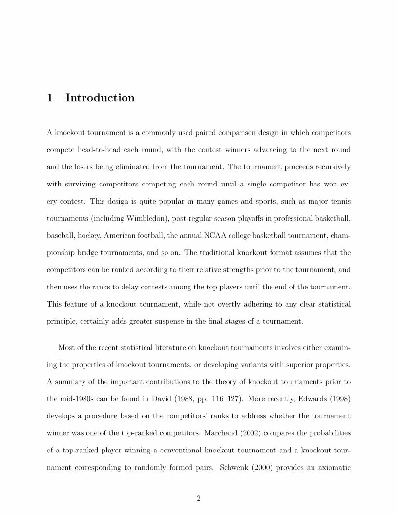
1 Introduction

A knockout tournament is a commonly used paired comparison design in which competitors

compete head-to-head each round, with the contest winners advancing to the next round

and the losers being eliminated from the tournament. The tournament proceeds recursively

with surviving competitors competing each round until a single competitor has won ev-

ery contest. This design is quite popular in many games and sports, such as major tennis

tournaments (including Wimbledon), post-regular season playoffs in professional basketball,

baseball, hockey, American football, the annual NCAA college basketball tournament, cham-

pionship bridge tournaments, and so on. The traditional knockout format assumes that the

competitors can be ranked according to their relative strengths prior to the tournament, and

then uses the ranks to delay contests among the top players until the end of the tournament.

This feature of a knockout tournament, while not overtly adhering to any clear statistical

principle, certainly adds greater suspense in the final stages of a tournament.

Most of the recent statistical literature on knockout tournaments involves either examin-

ing the properties of knockout tournaments, or developing variants with superior properties.

A summary of the important contributions to the theory of knockout tournaments prior to

the mid-1980s can be found in David (1988, pp. 116–127). More recently, Edwards (1998)

develops a procedure based on the competitors’ ranks to address whether the tournament

winner was one of the top-ranked competitors. Marchand (2002) compares the probabilities

of a top-ranked player winning a conventional knockout tournament and a knockout tour-

nament corresponding to randomly formed pairs. Schwenk (2000) provides an axiomatic

2

overview of knockout tournaments, and develops a variant to the conventional approach in-

volving randomizing the order of groups of players. The common theme in previous work

on designing knockout tournaments is that the information assumed to be available prior

to competition is either the relative ranks of the players, or all of the pairwise probabilities

that one competitor defeats another. These methods tacitly assume that relative strengths

of the competitors are known in advance, and that the only place for uncertainty are the

game outcomes. The starting point of this paper is to recognize not only that the statistical

purpose of a knockout tournament is to select the best competitor (see, for example, David,

1988, pg. 117), but that it is more realistic to assume only partial information about competi-

tors’ relative rankings rather than assuming relative strengths are completely known. To do

so, we posit an underlying probability model for game outcomes conditional on competitor

strengths, and assume that knowledge about the strengths can be asserted through a prior

distribution. The determination of pairings can then be framed as a Bayesian optimal design

problem, so that the optimal design can be viewed as a function of the prior distribution.

Bayesian optimal design as a framework for paired comparisons was originally proposed by

Glickman and Jensen (2005) who applied this approach to a setting involving balanced paired

comparison experiments. Specifically, their approach was designed to determine pairings

that maximized Kullback-Leibler information gain from the resulting game outcomes. This

approach is useful in paired comparison settings where efficiency is of primary interest;

for example, when the number of comparisons needs to be minimized to achieve maximal

expected information. In contrast, our approach involves a design criterion with the goal of

identifying the best player, which often is counter to the goal of increasing information.

3

This paper is organized as follows. We describe the paired comparison model and

Bayesian optimal design framework in Section 2. Within this section, we develop our optimal-

ity criterion, and describe the computations to solve the optimization problem. In Section 3,

we evaluate our method on simulated tournament data under a variety of settings, and com-

pare the results to other knockout formats. We conclude our paper in Section 4 by discussing

computational issues, alternative models, and open optimality issues.

2 Pairing approach

Suppose N = 2R players, for integer R > 1, are to compete in a R-round knockout tourna-

ment. In this format, N/2r contests take place in round r (r = 1, . . . , R), with the winners

advancing to the next round and the losers being eliminated. The winner of round R is

declared the tournament winner.

The approach we develop is intended to be applied adaptively, one round at a time,

and hence the method is only locally-optimal for the current round. We do not attempt to

optimize pairings over several rounds, or over the entire course of the tournament. This com-

promise approach emphasizes computational tractability, as exact optimization over more

than one round (or over the entire tournament) is likely to involve prohibitive computational

costs.

We assume the Thurstone-Mosteller model (Thurstone, 1927; Mosteller, 1951) for paired

comparison data. Specifically, we assume that for players i and j, with respective strength

4

parameters θi and θj, the probability player i defeats j is given by

πij = P(yij = 1 | θi, θj) = Φ(θi − θj), (1)

where yij is 1 if i defeats j and 0 if j defeats i, and Φ(·) is the standard normal distribution

function. Our framework assumes that ties or partial preferences are not permitted. For

notational convenience, yi will denote the game outcome relative to player i and πi will denote

the probability that player i wins (conditional on the strength parameters), suppressing the

indexing on the opponent.

Let θ = (θ1, . . . , θN) ∈ Θ ≡ <N denote the vector of N player strength parameters. Prior

to the tournament, we assume that knowledge about player strengths can be represented as

a multivariate normal distribution,

θ ∼ N(µ, Σ), (2)

where µ = (µ1, . . . , µN) is the vector of means, and Σ is the covariance matrix with diagonal

elements σ2i , and off-diagonal elements σij. Bayesian analysis of the Thurstone-Mosteller

model with a multivariate normal prior distribution can be implemented by recognizing its

reexpression as a probit regression (Critchlow and Fligner, 1991). Zellner and Rossi (1984)

discuss methods for Bayesian fitting of a probit model (as a specific instance of a generalized

linear model), including approximating the posterior distribution by a multivariate normal

density. Current Bayesian approaches to fitting probit (and other generalized linear) mod-

els rely on Markov chain Monte Carlo simulation from the posterior distribution; see, for

example, Dellaportas and Smith (1993).

The choice of the multivariate normal prior distribution is crucial to the tournament de-

5

sign problem. In some applications, especially those involving large communities of players

(including online or national gaming organizations), the multivariate normal prior distribu-

tion will usually factor into independent densities because covariance information on player

pairs is not typically reliable or worth saving due to storage constraints. Some sports ap-

plications in which teams compete during a regular season to gain entry into a post-season

elimination tournament (such as NFL football), a Thurstone-Mosteller model may be fit to

the regular season data, and the approximating normal posterior distribution (which now

consists of a covariance matrix with positive off-diagonal elements that were induced by the

regular season game outcomes) may be used as the prior distribution for the post-season

tournament.

With the incorporation of a multivariate normal prior distribution on the strength param-

eters, the (marginal) pairwise preference probabilities satisfy what David (1988, pg 5) terms

stochastic transitivity: For every set of three competitors i, j and k satisfying P(yij = 1) ≥ 12

and P(yjk = 1) ≥ 12, then

P(yik = 1) ≥ 1

2. (3)

This is trivially satisfied by our model, recognizing that when µi ≥ µj ≥ µk, stochastic

transitivity holds for all choices of a prior covariance matrix. The Thurstone-Mosteller model

with known strength parameters satisfies “strong stochastic transitivity,” which replaces (3)

with

P(yik = 1|θ) ≥ max(P(yij = 1|θ), P(yjk = 1|θ)). (4)

It is straightforward to demonstrate that our model incorporating the prior distribution does

not satisfy this stronger version: By selecting µi ≥ µj ≥ µk, setting the prior correlations of

6

(θi, θj) and of (θj, θk) to 1, setting the correlation of (θi, θk) to 0, and letting σ2i and σ2

k be

very large, P(yik = 1) can be made arbitrarily close to 12.

Following Lindley’s (1972, pg 19–20) Bayesian decision-theoretic framework for optimal

design, our approach involves specifying a utility function that is averaged over the data and

parameter space for the current round, and maximizing the expected utility over all possible

pairings. Particular to the tournament design problem, let S be the space of all pairings

of Nr players in round r of the tournament, and for a specific set of pairings s ∈ S, let Ys

be the collection of 2Nr/2 binary vectors y of potentially observable game outcomes. Our

general optimality criterion is to find s∗ that satisfies

U(s∗) = maxs∈S

∫Θ

∑y∈Ys

u(s,y,θ) p(y|θ) p(θ)dθ, (5)

where u(s,y,θ) is the utility for design s evaluated at data y and parameters θ, p(y|θ) is the

product of Thurstone-Mosteller probabilities of the game outcomes, p(θ) is the multivariate

normal prior density, and U(s) is the expected utility for design s averaged over both the data

and parameters. In Section 2.1, we present a specific utility function relevant to desirable

tournament outcomes, and demonstrate for fixed s the calculations of the expected utility

function. In Section 2.2, we describe a method for addressing tournaments in which the

number of competitors is not a power of 2, and an extension of our method that accounts for

order effects or a home-field advantage. For the development of our approach, we consider

the problem of determining first-round pairings of all N competitors, though our method

will apply to later rounds with fewer competitors remaining.

7

2.1 Optimization method

Our optimization strategy is to determine the set of pairings that maximizes the probability

the best player wins in the current round and thus advances to the next round. This criterion

is consistent with the goal of knockout tournaments to identify the best player, though it

is worthwhile to note that the criterion is being applied only to the current round of the

tournament. Let

i∗ = {i : θi ≥ θj, 1 ≤ j ≤ N}, (6)

so that i∗ indexes the best player. We want to find the set of pairings s∗ such that

P(yi∗ = 1 | s∗) ≥ P(yi∗ = 1 | s) (7)

for all s ∈ S. This criterion can be reexpressed in a utility framework in the following

manner. Define

Θi = {θ ∈ Θ : θi ≥ θj, all j 6= i}, (8)

that is, the subspace of Θ where θi is the largest. Note that⋃Ni=1 Θi = Θ, and P(Θi

⋂Θj) = 0

for i 6= j. The event that the best player wins can be written as the disjoint union

N⋃i=1

(yi = 1 ∩ θ ∈ Θi). (9)

Letting I{} be the event indicator function, the best-player utility function u for a design s

is given by

u(s,y,θ) = I{N⋃i=1

(yi = 1 ∩ θ ∈ Θi)}, (10)

and the corresponding expected utility is given by

U(s) =∫

Θ

∑y∈Ys

I{N⋃i=1

(yi = 1 ∩ θ ∈ Θi)} p(y|θ, s) p(θ)dθ

8

=∫

Θ

∑y∈Ys

N∑i=1

I{yi = 1 ∩ θ ∈ Θi} p(y|θ, s) p(θ)dθ

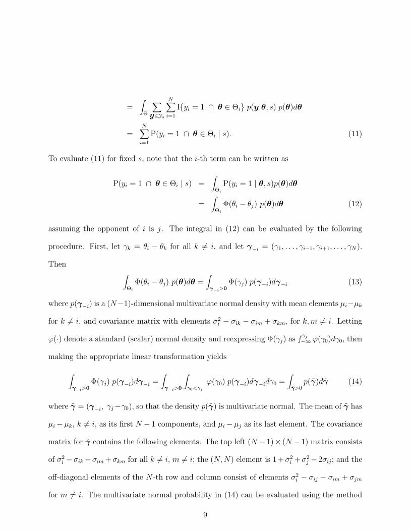
=N∑i=1

P(yi = 1 ∩ θ ∈ Θi | s). (11)

To evaluate (11) for fixed s, note that the i-th term can be written as

P(yi = 1 ∩ θ ∈ Θi | s) =∫

ΘiP(yi = 1 | θ, s)p(θ)dθ

=∫

ΘiΦ(θi − θj) p(θ)dθ (12)

assuming the opponent of i is j. The integral in (12) can be evaluated by the following

procedure. First, let γk = θi − θk for all k 6= i, and let γ−i = (γ1, . . . , γi−1, γi+1, . . . , γN).

Then ∫Θi

Φ(θi − θj) p(θ)dθ =∫γ−i>0

Φ(γj) p(γ−i)dγ−i (13)

where p(γ−i) is a (N−1)-dimensional multivariate normal density with mean elements µi−µk

for k 6= i, and covariance matrix with elements σ2i − σik − σim + σkm, for k,m 6= i. Letting

ϕ(·) denote a standard (scalar) normal density and reexpressing Φ(γj) as∫ γj−∞ ϕ(γ0)dγ0, then

making the appropriate linear transformation yields

∫γ−i>0

Φ(γj) p(γ−i)dγ−i =∫γ−i>0

∫γ0<γj

ϕ(γ0) p(γ−i)dγ−idγ0 =∫γ>0

p(γ)dγ (14)

where γ = (γ−i, γj−γ0), so that the density p(γ) is multivariate normal. The mean of γ has

µi−µk, k 6= i, as its first N − 1 components, and µi−µj as its last element. The covariance

matrix for γ contains the following elements: The top left (N − 1)× (N − 1) matrix consists

of σ2i −σik−σim +σkm for all k 6= i, m 6= i; the (N,N) element is 1 +σ2

i +σ2j − 2σij; and the

off-diagonal elements of the N -th row and column consist of elements σ2i − σij − σim + σjm

for m 6= i. The multivariate normal probability in (14) can be evaluated using the method

9

described in Genz (1992), which involves transforming the integral into one bounded in a

unit hypercube.

Example 1: Consider a four-player tournament with players A, B, C, and D, with prior

distribution θAθBθCθD

∼N

0.090.03−0.03−0.09

,

0.3 0.0 0.0 0.00.0 0.3 0.0 0.00.0 0.0 0.3 0.00.0 0.0 0.0 0.3

Note that this particular prior distribution has variances that are equal with moderate mag-

nitude. The means are equally spaced, and close relative to the variances. The values of

P(yij = 1 ∩ θ ∈ Θi) are numerically computed and given in row i and column j of the

following matrix.

A B C D

ABCD

− 0.230 0.233 0.236

0.196 − 0.201 0.2040.168 0.170 − 0.1740.143 0.145 0.147 −

By inspection, the set of pairings that corresponds to the largest expected utility (as given

in (11)) is {(A,D), (B,C)}, as

0.236 + 0.201 + 0.170 + 0.143 = 0.750

is maximal. One intuition behind the optimal pairing is that the arguably best player (A)

is paired with the worst (D), thus maximizing the probability of a win for best player A.

Example 2: In a different four-player tournament, suppose the prior distribution for players

10

A, B, C, and D is given byθAθBθCθD

∼N

0.090.03−0.03−0.09

,

0.01 0.0 0.0 0.00.0 1.0 0.0 0.00.0 0.0 1.0 0.00.0 0.0 0.0 0.01

The prior means in the current example are identical to the preceding example, but players

A and D have precisely estimated strengths, and strengths of B and C are imprecisely

estimated. The values of P(yij = 1∩θ ∈ Θi) are given in row i and column j of the following

matrix.

A B C D

ABCD

− 0.200 0.201 0.155

0.284 − 0.310 0.3000.262 0.284 − 0.2760.014 0.020 0.020 −

For this example, the set of pairings corresponding to the largest expected utility is {(A,C), (B,D)},

as

0.201 + 0.300 + 0.262 + 0.020 = 0.783

is maximal. Interestingly, even though A has a higher prior mean strength than B, it is

more probable that B will defeat A and be the best (with probability 0.284) than vice versa

(with probability 0.200). This can be understood through evaluating numerically the P(Θi),

P(ΘA) = 0.264, P(ΘB) = 0.368

P(ΘC) = 0.341 P(ΘD) = 0.027,

so that the two players with large prior variances (B and C) have a greater probability of

being the best compared to player A. This is an artifact of player A’s strength being precisely

11

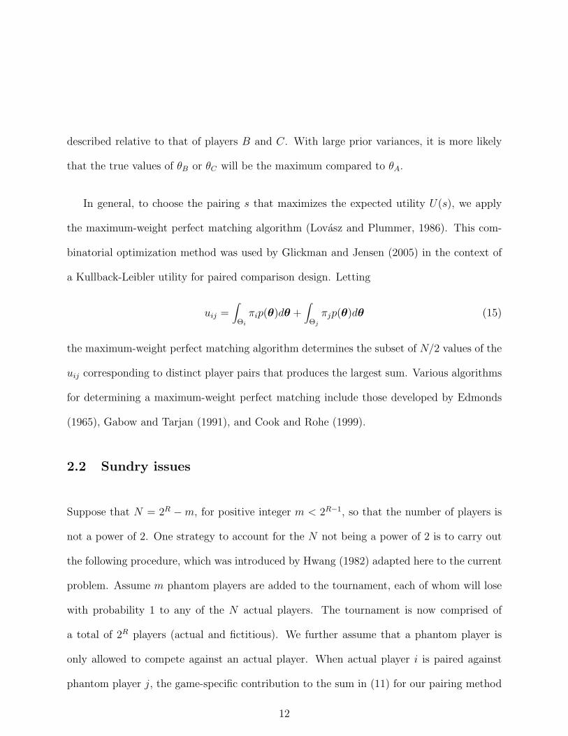
described relative to that of players B and C. With large prior variances, it is more likely

that the true values of θB or θC will be the maximum compared to θA.

In general, to choose the pairing s that maximizes the expected utility U(s), we apply

the maximum-weight perfect matching algorithm (Lovasz and Plummer, 1986). This com-

binatorial optimization method was used by Glickman and Jensen (2005) in the context of

a Kullback-Leibler utility for paired comparison design. Letting

uij =∫

Θiπip(θ)dθ +

∫Θjπjp(θ)dθ (15)

the maximum-weight perfect matching algorithm determines the subset of N/2 values of the

uij corresponding to distinct player pairs that produces the largest sum. Various algorithms

for determining a maximum-weight perfect matching include those developed by Edmonds

(1965), Gabow and Tarjan (1991), and Cook and Rohe (1999).

2.2 Sundry issues

Suppose that N = 2R −m, for positive integer m < 2R−1, so that the number of players is

not a power of 2. One strategy to account for the N not being a power of 2 is to carry out

the following procedure, which was introduced by Hwang (1982) adapted here to the current

problem. Assume m phantom players are added to the tournament, each of whom will lose

with probability 1 to any of the N actual players. The tournament is now comprised of

a total of 2R players (actual and fictitious). We further assume that a phantom player is

only allowed to compete against an actual player. When actual player i is paired against

phantom player j, the game-specific contribution to the sum in (11) for our pairing method

12

is P(Θi) for player i, and 0 for player j (as P(yi = 1 | θ) = 1, and P(yj = 1 | θ) = 0).

The expected utility can be calculated without any difficulty. The maximum-weight perfect

matching algorithm is then applied to all 2R players; actual players who are paired against

phantoms are awarded “byes” and automatically advance to the next round. This particular

procedure guarantees that the number of players in the subsequent round will then be a

power of 2.

It is often the case that one team or player has an advantage from playing on one’s

home field, or from having the first move in a game involving alternating turns (e.g., playing

white in chess). This type of advantage can be modeled in the Thurstone-Mosteller model

as an additive effect following Harris (1957); when i and j compete on the home field of

i, a home-field advantage parameter η increases the probability of a win for i by letting

πij = Φ(θi − θj + η). Assuming a normal prior distribution on η (which can be inferred,

for example, from previous game outcomes), one formal way to incorporate knowledge of

a home-field advantage is to compute the uij for each player pair (i, j) in two ways – once

when i has the home field advantage, and once when j has the home field advantage. This

computation recognizes that, for player i having the home-field advantage,

P(yi = 1 ∩ θ ∈ Θi | s) =∫

ΘiΦ(θi − θj + η) p(θ)dθ

which can then be computed in analogous manner to the method to evaluate equation (12).

Once each pair of uij are computed, the maximum-weight perfect matching algorithm can

be configured to consider only appropriate candidate solutions, for example by disallowing

pairing players with themselves. In future rounds of a tournament, where balance of home-

field frequency may be of interest, certain competitors can be forced to play either home or

13

away in a given round, with the perfect matching algorithm incorporating such constraints.

3 Evaluation of pairing methods

We evaluated our pairing method based on simulated tournament outcomes, and compared

it to other existing methods. In applying our approach, we did not adaptively update the dis-

tribution of strength parameters from the game outcomes; see Section 4 for further discussion

of this issue. In addition to our approach, we examined four other pairing methods. The first

was pairing at random. The second was standard knockout pairing scheme, which we briefly

outline below. The third and fourth methods were variants of the standard knockout format.

All methods (except random pairings) assume a relative ranking prior to competition. For

the non-model based approaches, the relative rankings prior to the tournaments are based

on the rankings of the µi. Because the marginal preference probabilities under our model

follow stochastic transitivity consistent with the ordering of the µi, then a pre-tournament

ranking is unambiguous (David, 1988, pg. 6).

The standard knockout format can be understood through a recursive construction. As-

sume N = 2R players at the start of the tournament. For round r = 1, . . . , R, the following

two steps are repeated:

1. Pair the players as {(k, 2R−r+1 + 1− k), k = 1, . . . , 2R−r}.

2. Relabel the winners within each pair as having the higher rank (i.e., the lower player

number); e.g., for the pair (3, 6), the winner of the contest is labeled “3.” This ensures

14

that the winners of round r are relabeled {1, 2, . . . , 2R−r}.

It is worth noting that the standard knockout design is a rooted binary tree in which the

terminal nodes are fixed at the start of the tournament. This feature of the design, while

ensuring a simple and easily implementable schedule, restricts many potential pairings from

occurring. This restriction can be viewed as a disadvantage to the standard method relative

to competitor approaches.

Two variants that have attempted to improve on the standard format are by Schwenk

(2000) and Hwang (1982). Schwenk’s approach is to apply the standard knockout format,

but first randomizing the ordering of competitors within particular groups. More specif-

ically, if we let Gr = {2r + 1, . . . , 2r+1} for r = 1, . . . , R − 1, then Schwenk proposes

to permute indices randomly within each Gr separately, relabel the indices in sorted or-

der, and then apply the standard format to the relabeled players. For example, in an

8-player tournament, in which the standard format would have the first-round pairings

{(1, 8), (2, 7), (3, 6), (4, 5)}, Schwenk’s approach involves randomly permuting elements of

G1 = {3, 4} and G2 = {5, 6, 7, 8} before applying the standard knockout format. The motiva-

tion for Schwenk’s approach is that monotonicity in the probability of winning a tournament

can be violated using standard pairings, i.e., one can construct preference probabilities in

which the probability that the highest ranked player wins the tournament is worse than the

second highest ranked player. Schwenk concludes that, based on several proposed axioms,

his method produces the fairest set of pairings, on average.

The variant by Hwang (1982) involves reseeding players after each round. The change

15

in the two-step algorithm in the standard format is to replace the relabeling step. Instead

of relabeling the winner within a pair to have the higher rank, the entire set of winners

is relabeled in sorted order. For example, the pairings for the first round of an 8-player

tournament are {(1, 8), (2, 7), (3, 6), (4, 5)}. If the winners are {1, 7, 3, 4}, then the standard

format would produce second-round pairings {(1, 4), (7, 3)} (after relabeling the “7” as “2”).

With Hwang’s approach, these four players are first sorted into {1, 3, 4, 7}, and then paired

via the standard format using the sorted order; the second-round pairing would then be

{(1, 7), (3, 4)}.

We simulated 16-player knockout tournaments, each requiring four rounds to determine

the winner. Our simulation experiment involved generating tournament outcomes using

six different assumed prior distributions for θ. To generate data for a single tournament

given a prior distribution, we first simulate a single vector θ, the true strengths, from the

prior distribution. Game outcomes within an individual tournament were then simulated

in the following manner. For i = 1, . . . , 16 and r = 1, . . . , 4, we simulated Xir ∼ N(θi,12)

independently. Let X denote the 16 by 4 matrix of simulated Xir. In round r, if players j

and k are paired, then j is declared the winner if Xjr > Xkr, and k the winner otherwise.

This data-generating process ensures not only that the Thurstone-Mosteller probabilities

are consistent with the simulated θi, but that several tournament design algorithms can be

evaluated on the same simulated data despite different formation of pairs.

We considered six simulation scenarios, corresponding to six different prior distributions.

In each scenario, we assumed that the largest difference µi − µj was 1.5. If player strengths

were equal to the means, the probability that the top player defeats the bottom player is

16

Φ(θ1 − θ16) = Φ(1.5) = 0.933. In the first five scenarios, the µi, i = 1, . . . , 16, are equally

spaced, and in the sixth scenario the top 12 players and bottom four players are separated

by large margin. In all scenarios, we assumed a multivariate normal prior distribution that

factored into independent densities. The specific choices of µi and σ2i are as follows.

(A) µi = 0.75− 0.1(i− 1); σ2i = 0.1, for all i

(B) µi = 0.75− 0.1(i− 1); σ2i = 0.01 for odd i, and σ2

i = 1.0 for even i

(C) µi = 0.75− 0.1(i− 1); σ2i = 0.01 for i ≤ 8, and σ2

i = 1.0 for i ≥ 9

(D) µi = 0.75− 0.1(i− 1); σ2i = 1.0 for i ≤ 8, and σ2

i = 0.01 for i ≥ 9.

(E) µi = 0.75− 0.1(i− 1); σ2i = 0.01 for i ≤ 4, and σ2

i = 1.0 for i ≥ 5

(F) µi = 0.75 − 0.01(i − 1) for i = 1, . . . , 12, µi = −0.60 − 0.05(i − 13) for i = 13, . . . , 16;

σ2i = 0.01 for i ≤ 8, and σ2

i = 1.0 for i ≥ 9

Scenario (A) corresponds to equally spaced strengths with equal and moderate uncertainty

in θ. Scenario (B) alternates low and high uncertainty across the θi. Scenario (C) assumes

that the top half of the players have precisely described strengths, but the bottom half are

uncertain, whereas scenario (D) is the reverse of (C). Scenario (E) is the same as (C), except

that only the first four players have low uncertainty in θ. Finally, Scenario (F) has the first

12 players with equally spaced µi between 0.75 and 0.64 and the bottom four equally spaced

between −0.6 and −0.75, and the top half of the players have precisely described strengths

but the bottom half are uncertain.

17

From each of the six assumed prior distributions, we generated 10,000 sets of θ and X. We

then applied the five tournament design algorithms and recorded the rank of θi for the tour-

nament winner. The maximum-weight perfect matching algorithm for our two methods was

implemented using publicly available C code by Ed Rothberg (which can be downloaded from

http://elib.zib.de/pub/Packages/mathprog/matching/weighted/) that implements Gabow’s

(1973) algorithm. The results of the simulations are summarized in Table 1. The entries

within each column are the proportion of simulated tournaments in which tournament win-

ner was the player with the highest θi, the proportion in which the winner was the second

best (according to the simulated θi), and so on.

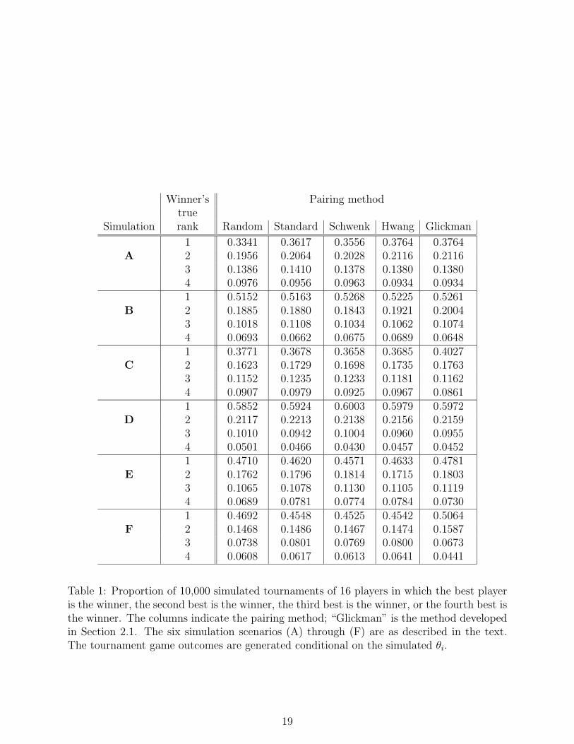
The simulations demonstrate that the approach developed in Section 2.1, labeled “Glick-

man” on Table 1, competes well against the other methods. In simulation (A), where the

σ2i are the same for all players, our method performs at least as well as all competitor meth-

ods, and coincides exactly with Hwang’s method in this case. It is worth mentioning that

Hwang’s approach coincides with our approach when the σ2i are equal and small, but there

are cases with equal but larger σ2i where the two approaches do not coincide (though they

are nonetheless competitive with each other). In simulation (B) where the magnitude of the

variances alternate, our method outperforms most other methods (except Schwenk’s) but

not by a large or practical margin. However this does suggest that situations in which the

prior variances vary may lead to our method potentially outperforming competitor methods.

In simulations (C) and (D), we investigated the impact of the top players’ strengths being

precise, and the bottom players’ strengths being precise, respectively. From the simulation

results, our method performs no better than competitor methods when the top players’

18

Winner’s Pairing methodtrue

Simulation rank Random Standard Schwenk Hwang Glickman

1 0.3341 0.3617 0.3556 0.3764 0.3764A 2 0.1956 0.2064 0.2028 0.2116 0.2116

3 0.1386 0.1410 0.1378 0.1380 0.13804 0.0976 0.0956 0.0963 0.0934 0.09341 0.5152 0.5163 0.5268 0.5225 0.5261

B 2 0.1885 0.1880 0.1843 0.1921 0.20043 0.1018 0.1108 0.1034 0.1062 0.10744 0.0693 0.0662 0.0675 0.0689 0.06481 0.3771 0.3678 0.3658 0.3685 0.4027

C 2 0.1623 0.1729 0.1698 0.1735 0.17633 0.1152 0.1235 0.1233 0.1181 0.11624 0.0907 0.0979 0.0925 0.0967 0.08611 0.5852 0.5924 0.6003 0.5979 0.5972

D 2 0.2117 0.2213 0.2138 0.2156 0.21593 0.1010 0.0942 0.1004 0.0960 0.09554 0.0501 0.0466 0.0430 0.0457 0.04521 0.4710 0.4620 0.4571 0.4633 0.4781

E 2 0.1762 0.1796 0.1814 0.1715 0.18033 0.1065 0.1078 0.1130 0.1105 0.11194 0.0689 0.0781 0.0774 0.0784 0.07301 0.4692 0.4548 0.4525 0.4542 0.5064

F 2 0.1468 0.1486 0.1467 0.1474 0.15873 0.0738 0.0801 0.0769 0.0800 0.06734 0.0608 0.0617 0.0613 0.0641 0.0441

Table 1: Proportion of 10,000 simulated tournaments of 16 players in which the best playeris the winner, the second best is the winner, the third best is the winner, or the fourth best isthe winner. The columns indicate the pairing method; “Glickman” is the method developedin Section 2.1. The six simulation scenarios (A) through (F) are as described in the text.The tournament game outcomes are generated conditional on the simulated θi.

19

strengths are uncertain and the bottom players’ are precise (simulation (D)). But in simula-

tion (C), where the top players’ strengths are precise, our method substantially outperforms

competitor methods, including Hwang’s. In the spirit of McNemar’s (1947) procedure, the

difference in probabilities of the tournaments identifying the best player using our method

versus Hwang’s is “significantly” positive. The results of simulation (E), in which only the

top four players have precise strengths, are not as strong as in simulation (C), though in this

case our method still outperforms all others (and significantly so based on a McNemar pro-

cedure for the comparison against Hwang’s method). Simulation (F) is much like simulation

(C) in that the top half of players have precise strengths and the bottom half are imprecise,

but that the means are not equally spaced. It appears that the non-uniform separation in

means does not detract from our method’s clearly outperforming the competitor methods.

The implication is that scenarios where the better players have precisely estimated strengths

and weaker players have imprecisely estimated strengths are ones that evidence the advan-

tages of our method. It is interesting to note in simulation (F) that random pairings tend

to outperform standard, Schwenk’s and Hwang’s methods in having the tournament winner

be the best a prior, though random pairings do not outperform these three other methods

in having the tournament winner be one of the top two (that is, adding the first and second

rows on Table 1 within simulation (F)).

It is also interesting to note that, compared to other methods, the frequency of the tour-

nament winner being the second, third or fourth best player is no worse than the analogous

frequencies for other methods. Thus, cumulatively, our method is competitive in having the

tournament winner be one of the top players if not the outright best.

20

4 Discussion

Based on the simulations, it appears that the Bayesian optimal design approach leads to

competitor pairings that are consistent with a high probability of singling out the best

player. Our method, which optimizes the probability that the best player wins in the current

round, appears through our simulation analyses to be at least as promising, in general, as all

competitor approaches considered here. This approach seems to perform especially well when

the top players’ strengths are precisely estimated, and the bottom players are imprecisely

estimated. In gaming organizations, it is often the case that the best players compete

more frequently than weaker players and therefore have strengths that are more precisely

estimated, so that our pairing method would be ideal for such a scenario. Even in scenarios

where players have strengths with similar precision, our method tends to coincide with

standard types of seeding approaches, thereby providing a probabilistic justification of these

common but ad-hoc approaches to pairing competitors in knockout tournaments. While

our method performs quite well, it can be computationally intensive, requiring N(N − 1)

evaluations of an N -variate normal probability prior to invoking the maximum-weight perfect

matching algorithm.

In practice, gaming organizations or leagues of competitors rarely compute the type of

information that is assumed in the method developed in this paper. At best, competitors are

seeded in tournaments from rankings that are based on crude summaries, such as placement

on competitive ladders, or the tournament monetary earnings over a fixed time period. Even

in situations where organizations adopt probabilistic rating systems, such as in competitive

21

chess, the seeding methods for tournaments are determined from simple summaries, often

using standard pairing methods. Given that the current culture is to keep seeding methods

simplistic, can an approach such as the one developed here make its way into practice?

In order for this to happen, statisticians need to educate sports and gaming organizations

about the benefits of fitting (relatively simple) statistical models and summarizing not only

individual strength estimates, but also measures of uncertainty. This type of complexity

is present in recent rating systems; the approaches in Glickman (1999), Glickman (2001),

and Herbrich and Graepel (2006), all of which determine a normal posterior distribution of

playing strengths through approximate Bayesian filters, have been adopted by commercial

gaming organizations. Given that headway is being made in complex systems for rating

competitors from game outcomes, perhaps equally computationally intensive tournament

design systems with desirable statistical properties will also make their way into practice.

In using a Bayesian framework, it is tempting to update the prior distribution after

each round of a tournament, and then applying our pairing approach based on the posterior

distribution from the previous round. The problem with this approach is related to the non-

random aspect of the pairing method. The drawback is that the result of a single game per

player can lead to a posterior distribution with undesirable features. For example, suppose

that the top player is paired against the bottom player, and player N/2 is paired against

N/2 + 1, with the higher ranked player winning. In this situation, it is reasonable to expect

that the posterior mean strength for the top player will not be much higher than the prior

mean, but that the posterior mean strength for the N/2 player could increase substantially

(because this player defeated someone of similar strength). It is not unreasonable to imagine

22

that the posterior mean strengths of the top-ranked and middle player would switch relative

to the prior means.

Our methodology could be adapted to the more commonly used Bradley-Terry (1952)

model, though this would require additional approximations in the computation. The

Bradley-Terry model assumes that P(yij = 1|θi, θj) = 1/(1+exp(−(θi−θj))), a logistic distri-

bution function of the difference in players’ strengths. This substitution into (12) complicates

the calculation because the computation involves evaluating an integral of a logistic distribu-

tion function with respect to a truncated multivariate normal density. Instead, an approach

that has been explored involves reexpressing summands in (11) as P(Θi|yi = 1)P(yi = 1),

where the first factor is calculated by approximating the posterior density, p(θ|yi = 1), by a

multivariate normal distribution, and then evaluating the integral, while the second factor,

which involves an integral over a scalar variable, can be computed numerically using Gauss-

Hermite quadrature (see, for example, Davis and Rabinowitz, 1975; Crouch and Spiegelman,

1990; Press et al., 1997). The difficulty is that evaluating the first integral as a normal

probability calculation can be unreliable, especially if the prior density represents weak in-

formation. In this instance, the single game outcome yi = 1 can result in a posterior density

that is poorly approximated by a normal distribution.

Direct application of our approach is limited to tournaments with only one contest per

pair. This is appropriate for post-regular season playoffs in sports such as NFL football, but

not for playoffs in NHL hockey or NBA basketball, both of which involve playing a best-of-

seven game series (that is, the first team to win four games advances). One approach towards

pairing teams for series competition within the context of our framework is to respecify a

23

Thurstone-Mosteller model for winning an entire series as opposed to a single game, and

approximating the parameters of a normal prior distribution for the Thurstone-Mosteller

model from the single-game normal prior distribution. The pairing method developed here

can then be applied to the resulting prior distribution. The method of approximating the

multiple-game prior distribution is an open question, and beyond the scope of this paper.

It is worth noting that our method is a “greedy” algorithm, satisfying optimality con-

ditions on a round-at-a-time basis. This does not imply global optimality. Example 2 in

Section 2.1 illustrates this issue. The optimal pairing by our method for the first round is de-

termined to be {(A,C), (B,D)}, which conveys a 0.783 probability that the best player wins

in the current round. If the pairing were the standard pairing {(A,D), (B,C)}, the proba-

bility that the best player wins the current round would be 0.763. However, the probability

that the best player wins the entire 4-player tournament with the pairings {(A,C), (B,D)},

is computed to be 0.582, while with {(A,D), (B,C)} the probability is 0.592. Thus, in this

example, our method does not maximize the probability that the best player will win the

entire tournament.

Despite the lack of global optimality properties, our approach does seem to work well

empirically. Our approach to the design of knockout tournaments takes advantage of in-

formation known prior to competition, and then uses an optimality criterion to determine

a set of pairings. The ability both to describe optimality conditions based on the strength

parameters, as well as being able to specify a prior distribution on these parameters, allows

great flexibility and power as a design framework for knockout tournaments.

24

References

Bradley R. A., Terry, M. E., 1952. “The rank analysis of incomplete block designs. 1. Themethod of paired comparisons.” Biometrika, 39, 324–45.

Cook, W.J., Rohe, A., 1999. “Computing minimum-weight perfect matchings.” INFORMSJournal on Computing, 11, 138–148.

Critchlow, D.E., Fligner, M.A., 1991. “Paired comparison, triple comparison, and rankingexperiments as generalized linear models, and their implementation in GLIM.” Psychome-trika, 56, 517–533.

Crouch, E.A.C., Spiegelman, D., 1990. “The evaluation of integrals of the form∫f(t) exp(−t2)dt:

application to logistic normal models.” Journal of the American Statistical Association,85, 464–9.

David, H. A., 1988. The method of paired comparisons (2nd ed.). Chapman and Hall,London.

Davis, P.J., Rabinowitz, P., 1975. Methods of numerical integration. Dover, New York.

Dellaportas, P., Smith, A.F.M., 1993. “Bayesian inference for generalized linear and propor-tional hazards models via Gibbs sampling.” Applied Statistics, 42, 443–459.

Edmonds, J., 1965. “Paths, trees and flowers.” Canadian Journal of Mathematics, 17,449–467.

Edwards, C.T., 1998. “Non-parametric procedure for knockout tournaments.” Journal ofApplied Statistics, 25, 375–385.

Gabow, H.N., 1973. “Implementation of algorithms for maximum matching on nonbipartitegraphs.” Ph.D. Thesis, Stanford University.

Gabow, H.N., Tarjan, R.E., 1991. “Faster scaling algorithms for general graph matchingproblems.” Journal of the ACM, 38, 815–853.

Genz, A., 1992. “Numerical computation of multivariate normal probabilities.” Journal ofComputational and Graphical Statistics, 1, 141–149.

Glickman, M.E., 1999. “Parameter estimation in large dynamic paired comparison experi-ments.” Applied Statistics, 48, 377–394.

25

Glickman, M.E., 2001. “Dynamic paired comparison models with stochastic variances.”Journal of Applied Statistics, 28, 673–689.

Glickman, M.E., Jensen, S.T., 2005. “Adaptive paired comparison design.” Journal ofStatistical Planning and Inference, 127, 279–293.

Harris, W.P., 1957. “A revised law of comparative judgment.” Psychometrika, 22, 189–198.

Herbrich, R., Graepel, T. 2006. “TrueSkillTM : A Bayesian skill rating system.” Technicalreport MSR-TR-2006-80, Microsoft Research.

Hwang, F.K., 1982. “New concepts in seeding knockout tournaments.” American Mathe-matical Monthly, 89, 235–239.

Lindley, D.V., 1972. Bayesian statistics – a review. SIAM, Philadelphia.

Lovasz, L., Plummer, M.D., 1986. Matching theory. Akademia i Kiadoo, Budapest.

Marchand, E., 2002. “On the comparison between standard and random knockout tourna-ments.” The Statistician, 51, 169–178.

McNemar, Q., 1947. “Note of the sampling error of the difference between correlated pro-portions or percentages.” Psychometrika, 12, 153–157.

Mosteller, F., 1951. “Remarks on the method of paired comparisons: I. The least squaressolution assuming equal standard deviations and equal correlations.” Psychometrika, 16,3–9.

Press, W.H., Teukolsky, S.A., Vetterling, W.T., Flannery, B.P., 1997. Numerical recipes inFortran 77: The art of scientific computing (2nd ed). Cambridge University Press, NewYork.

Schwenk, A.J., 2000. “What is the correct way to seed a knockout tournament?” AmericanMathematical Monthly, 107, 140–150.

Thurstone, L.L., 1927. “A law of comparative judgment.” Psychological Review, 34, 273–286.

Zellner, A., Rossi, P.E., 1984. “Bayesian Analysis of Dichotomous Quantal Response Mod-els.” Journal of Econometrics, 25, 365–393.

26