6/1/14  

1  

Bayesian methods!Recall Bayes’ formula!!!!!!!In the context of continuous random variables X and Y this becomes!

34

P(Ai B) =P(B Ai)P(Ai )

P(B Aj)P(Aj )j=1

n

∑

fY X (y x) =fX Y (x y)fY (y)fX Y (x u)fY (u)du∫

Expressing uncertainty!In the Bayesian approach to statistic we describe anything that is uncertain by a probability distribution. !The likelihood is the conditional distribution of data X given the parameter (now a random variable) :!!!Before we collect data we assign a prior distribution to :!!After observing data x, we compute the posterior distribution of : ! !

35

L(θ) = fXΘ (x θ)

fΘ (θ)

fΘ X (θ x)

Θ

Θ

Θ

Some history!

Thomas Bayes 1701-1761

Dennis Lindley 1923 – 2013

Pierre-Simon Laplace 1749–1827

Harold Jeffries 1891-1989

George Box 1919–2013

Where does the prior come from?!

Previous experience!Expert knowledge!Mathematical convenience!!The posterior depends on the prior.!But if you have a lot of data, the posterior will look similar to the likelihood.!

37

6/1/14  

2  

Production!The error rate in production of a computer chip is about 9%. The proportion P of faulty chips has a prior distribution proportional to p10(1-p)90. !From a large batch, we sample 100 chips and find 16 defective.!L(p) = !!f(p|x) = !

38 39

0.0 0.2 0.4 0.6 0.8 1.0

05

1015

20p

density

0.0 0.2 0.4 0.6 0.8 1.0

05

1015

20p

density

0.0 0.2 0.4 0.6 0.8 1.0

05

1015

20p

density

prior post

mode 0.09 0.145

sd 0.030 0.024

What if we make another experiment?!

Use the posterior from the past experiment as the prior for the new one.!This is the same as using the original prior and then performing the combined experiment.!

40

Last Friday lecture!Bayesian statistics!Prior and posterior!Updating posterior!

41

6/1/14  

3  

Friday problems!1. Under H0 X~Bin(16,.5) so P(X≥11)=.105!2.!!!!!!!!Hence the expected table is!5.97 !16.19 !21.72 !16.12!8.95 !24.28 !32.58 !24.18!and the chi-square statistic is 15.84 more than ! 42

µ̂ = 60 × 1.954 + 90 × 2.616150

= 2.3512

xi2∑ = 59 × .3332 + 60 × 1.9542 = 235.6294

yi2∑ = 89 × 1.2702 + 90 × 2.6162 = 759.4591

σ̂2 = 1149 ( xi2∑ + yi2∑ − 150 × 2.35122 ) = 1.106

σ̂ = 1.052

χ.952 (3 + 3 − 2) = 9.49

3. (a) At the boundary between the hypothesis Y=# negative Xi ~ Bin(19,0.4)!We would reject for small values of Y. The critical region would be Y≤3, since P(Y≤3)=.023 and P(Y≤4)=.069. The power is P(Y≤3;p=0.2)=0.46!(b) P(X<0)=Φ(-μ)=0.4 so μ=0.253. By sufficiency our test statistic will be ΣXi, and we reject for large values. So!!and C=2.75. p=0.2 corresponds to μ=0.842 and the power is!!!4. (a) θ=1,...,6 with P(θ=k)=(2k-1)/36!(b) P(X=x|θ)=1/θ,x=1,...,θ!(c) P(θ=k|X=4)=c(2k-1)/36×1/k, max for k=6 (d) L(θ)=1/θ, θ≥x so max at θ=4! 43

α = P( Xi > C) = 1− Φ((C − 0.253) / 19)∑

P( Xi∑ > 2.75) = 1− Φ(2.7519

− .842) = 0.80

Exponential case!Let the prior be Exp(𝜶) and the data ) and the data Exp(𝝀). Then the posterior is!). Then the posterior is!!!!This is a gamma density with shape parameter (n+1) and scale parameter ∑xi+𝜶. !. !𝜶 is called a hyperparameter, and is set is called a hyperparameter, and is set by the statistician based on prior expectations.!!

44

f(λ x) ∝ αλn exp −λ xi + αi=1

n

∑⎛⎝⎜⎞⎠⎟

⎧⎨⎩

⎫⎬⎭

Conjugate priors!A mathematically convenient prior is one where the prior and posterior are in the same parametric family.!Poisson likelihood:!!!If we look at things involving x’s (or n) as parameters, and things involving 𝛌 as as the dummy variable, we choose a prior of the form ! ! ! ! ! ! which is a gamma density. Then the posterior density will also be gamma, with shape parameter ! ! and shape parameter β+n. ! 45

L(λ) = λxi

i=1

n

∑exp(−nλ)

f(λ) ∝ λα exp(−βλ)

α + xi∑

6/1/14  

4  

Some conjugate priors!

Likelihood Prior Posterior Gamma/Exponential

Gamma/Exponential

Gamma

Poisson Gamma/Exponential

Gamma

Binomial Beta/Uniform Beta Normal, known variance

Normal Normal

46

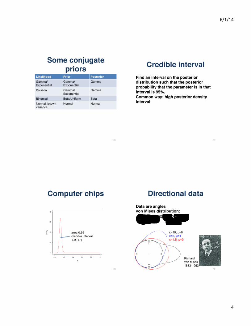
Credible interval!Find an interval on the posterior distribution such that the posterior probability that the parameter is in that interval is 95%.!Common way: high posterior density interval!

47

Computer chips!

0.0 0.2 0.4 0.6 0.8 1.0

05

1015

20

p

density

48

area 0.95 credible interval (.9,.17)

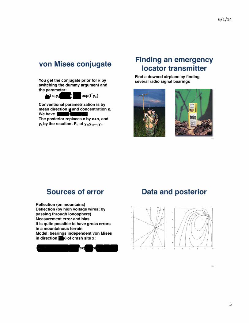
Directional data!Data are angles!von Mises distribution:!

49

f(θ µ,κ) == exp(κcos(θ − µ))2πI0 (κ)

0

π

2

π

3π2

+

κ=10, µ=0 κ=5, µ=1 κ=1.5, µ=0

Richard von Mises 1883-1953

6/1/14  

5  

von Mises conjugate!

You get the conjugate prior for κ by switching the dummy argument and the parameter:!!!Conventional parametrization is by mean direction μ and concentration κ.!We have !The posterior replaces c by c+n, and y0 by the resultant Rn of y0,y1,...,yn.!

fτ (t c,y0 ) ∝ I0 ( t )⎡⎣ ⎤⎦−c exp(tTy0 )

µy = (κ cosθ,κ sinθ)

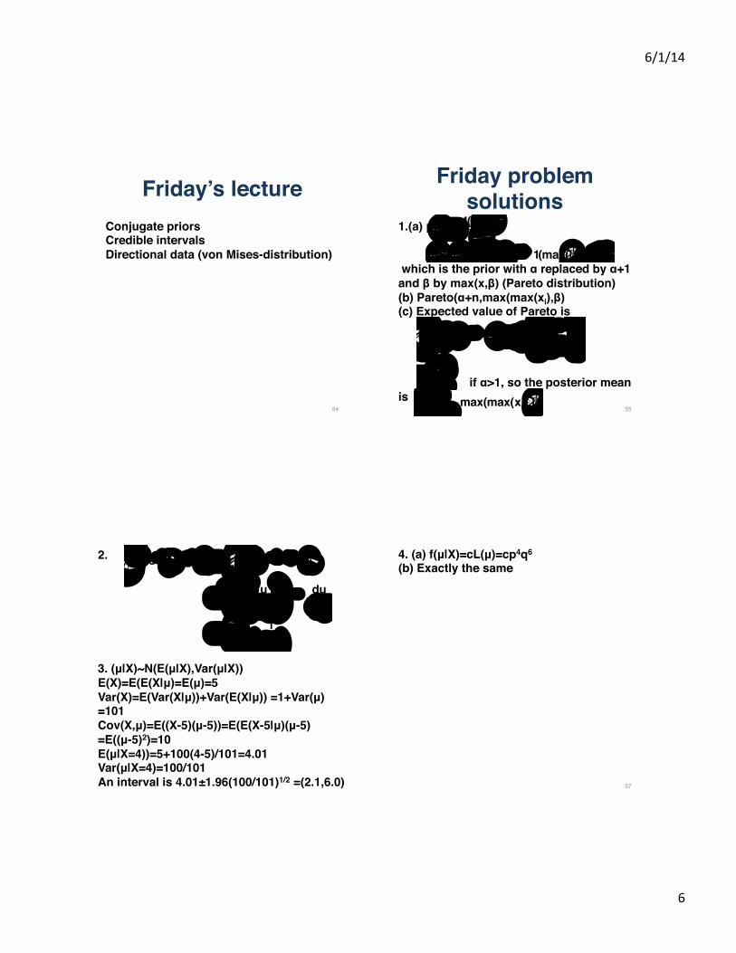
Finding an emergency locator transmitter!

Find a downed airplane by finding several radio signal bearings!

51

Sources of error!Reflection (on mountains)!Deflection (by high voltage wires; by passing through ionosphere)!Measurement error and bias!It is quite possible to have gross errors in a mountainous terrain!Model: bearings independent von Mises in direction of crash site x:!!f(θi µ i,κ,β) = 2π I0 (κ)[ ]−1exp(κcos(θi − µ i − β))

µ i (x)

Data and posterior!

53

6/1/14  

6  

Friday’s lecture!Conjugate priors!Credible intervals!Directional data (von Mises-distribution)!

54

Friday problem solutions!

1.(a)!!! which is the prior with α replaced by α+1 and β by max(x,β) (Pareto distribution)!(b) Pareto(α+n,max(max(xi),β)!(c) Expected value of Pareto is!!!!!! ! ! !if α>1, so the posterior mean

is !! 55

L(θ) = 1(x ≤ θ)θ

f(θ)L(θ) ∝ αβαθ− (α+2)1(max(β,x) ≤ θ)

θαβαθ− (α+1) dθ = αβα θ− (α−1)

α − 1⎡⎣⎢

⎤⎦⎥β

∞

∫β

∞

= αβα − 1α + n

α + n − 1max(max(xi),β)

2.!!!!!!!!3. (μ|X)~N(E(μ|X),Var(μ|X))!E(X)=E(E(X|μ)=E(μ)=5!Var(X)=E(Var(X|μ))+Var(E(X|μ)) =1+Var(μ) =101!Cov(X,μ)=E((X-5)(μ-5))=E(E(X-5|μ)(μ-5)!=E((μ-5)2)=10!E(μ|X=4))=5+100(4-5)/101=4.01!Var(μ|X=4)=100/101!An interval is 4.01±1.96(100/101)1/2 !=(2.1,6.0)!

λx

x!∫ e −λ µe −µλdλ = 1x!

µλxe −λ (1+µ ) dλ∫

= µx!

u1+ µ

⎛⎝⎜

⎞⎠⎟∫x

e −u du1+ µ

= µ1+ µ

11+ µ( )x

4. (a) f(μ|X)=cL(μ)=cp4q6!

(b) Exactly the same!

57

6/1/14  

7  

Review!Regression!!Bivariate normal!!Simple linear regression!!Least squares!

!ANOVA!!Group comparison!!Decomposition of sum of squares!!!

Goodness of fit!!Chi-squared test!!Empirical df!!Kolmogorov-Smirnov test!!Q-Q-plot!

58