bayesian methods in reliability engineering -...
TRANSCRIPT

Bayesian Methods in Reliability Engineering
ASQ Reliability Division Webinar Program
Nov 15th 2012
Charles H. Recchia, MBA, PhD
Quality Support Group, Inc
http://www.qualitysupportgroup.com/

BAYESIAN METHODS IN RELIABILITY ENGINEERING With product reliability demonstration test planning and execution interacting
heavily with cost, availability and schedule considerations, Bayesian methods offer an intelligent way of incorporating engineering knowledge based on historical information into data analysis and interpretation, resulting in an overall more precise and less resource intensive failure rate estimation. This talk consists of three parts
Introduction to Bayesian vs Frequentist statistical approaches
Bayesian formalism for reliability estimation
Product/component case studies and examples
Charles Recchia has more than two dozen years of fundamental research, technology/product development, and management experience with a special focus on reliability statistics of complex systems. He earned a doctorate in Condensed Matter Physics from Ohio State University, and a Master of Business Administration degree from Babson College. Dr. Recchia accrued reliability engineering expertise at Intel, MKS Instruments and Saint-Gobain Innovative Materials R&D, has served as adjunct professor at Wittenberg University, and is author of numerous peer-reviewed technical papers and patents. He is a senior member of ASQ, the American Physical Society, and serves on the Advisory Committee for the Boston Chapter of the IEEE Reliability Society.
11/15/2012 ASQ RD Webinar 2
Agenda
• Bayesian vs. Frequentist Comparison
• Preliminary Example
• Conjugate Priors
• Test Time Examples
• Question and Answer
11/15/2012 ASQ RD Webinar 3

11/15/2012 ASQ RD Webinar 4

Agenda
• Bayesian vs. Frequentist Comparison
• Preliminary Example
• Conjugate Priors
• Test Time Examples
• Question and Answer
11/15/2012 ASQ RD Webinar 5

Agenda
• Bayesian vs. Frequentist Comparison
• Preliminary Example
• Conjugate Priors
• Test Time Examples
• Question and Answer
11/15/2012 ASQ RD Webinar 6
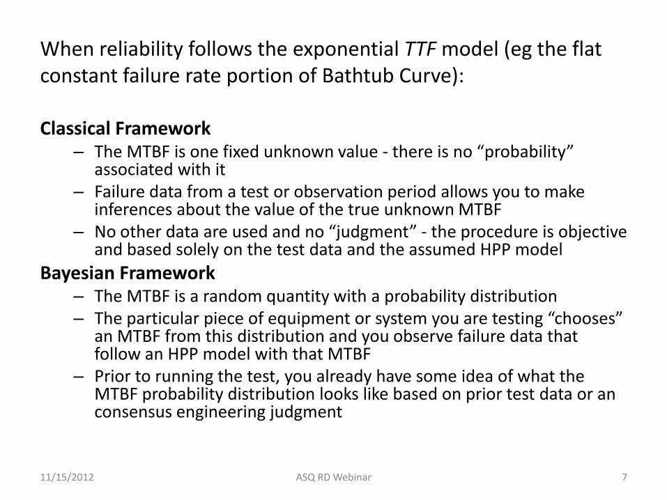
When reliability follows the exponential TTF model (eg the flat constant failure rate portion of Bathtub Curve):
Classical Framework – The MTBF is one fixed unknown value - there is no “probability”
associated with it – Failure data from a test or observation period allows you to make
inferences about the value of the true unknown MTBF – No other data are used and no “judgment” - the procedure is objective
and based solely on the test data and the assumed HPP model
Bayesian Framework – The MTBF is a random quantity with a probability distribution – The particular piece of equipment or system you are testing “chooses”
an MTBF from this distribution and you observe failure data that follow an HPP model with that MTBF
– Prior to running the test, you already have some idea of what the MTBF probability distribution looks like based on prior test data or an consensus engineering judgment
11/15/2012 ASQ RD Webinar 7

exponential distribution “non-intuitive”
Brains wired with
Normal Distribution s ~ 0.1m
5’9” 6’3” 5’10” 5’9” 6’0” 5’9”
Planet = Earth 6 draw sample. Population mean height 5’11” Sample mean = ______
8
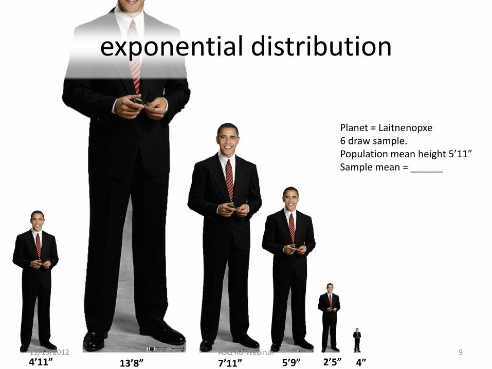
4’11” 13’8” 7’11” 5’9” 2’5” 4”
Planet = Laitnenopxe 6 draw sample. Population mean height 5’11” Sample mean = ______
exponential distribution
11/15/2012 ASQ RD Webinar 9

Confidence vs. Credibility Intervals
11/15/2012 ASQ RD Webinar 10

For and Against use of Bayesian Methodology PROs CONs
Uses prior information - this "makes sense“ Less new testing may be needed to confirm a desired MTBF at a given confidence Confidence intervals are really intervals for the (random) MTBF - sometimes called "credibility intervals“
Prior information may not be accurate - generating misleading conclusions Way of inputting prior information (choice of prior) may not be correct Customers may not accept validity of prior data or engineering judgements Risk of perception that results aren't objective and don't stand by themselves
11/15/2012 ASQ RD Webinar 11
Agenda
• Bayesian vs. Frequentist Comparison
• Preliminary Example
• Conjugate Priors
• Test Time Examples
• Question and Answer
11/15/2012 ASQ RD Webinar 12

Agenda
• Bayesian vs. Frequentist Comparison
• Preliminary Example
• Conjugate Priors
• Test Time Examples
• Question and Answer
11/15/2012 ASQ RD Webinar 13
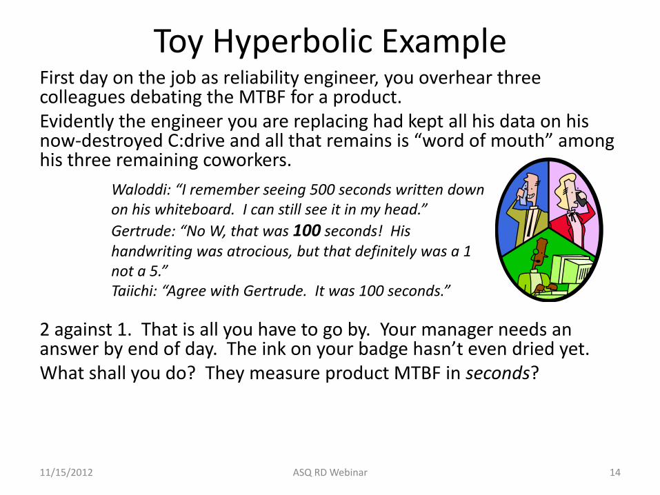
Toy Hyperbolic Example First day on the job as reliability engineer, you overhear three colleagues debating the MTBF for a product. Evidently the engineer you are replacing had kept all his data on his now-destroyed C:drive and all that remains is “word of mouth” among his three remaining coworkers. 2 against 1. That is all you have to go by. Your manager needs an answer by end of day. The ink on your badge hasn’t even dried yet. What shall you do? They measure product MTBF in seconds?
Waloddi: “I remember seeing 500 seconds written down on his whiteboard. I can still see it in my head.”
Gertrude: “No W, that was 100 seconds! His handwriting was atrocious, but that definitely was a 1 not a 5.” Taiichi: “Agree with Gertrude. It was 100 seconds.”
11/15/2012 ASQ RD Webinar 14

Bayesian Core Idea
What you knew before WYKB.
“Prior” New Data
Best possible update of WYKB adjusted by the New Data.
“Posterior”
11/15/2012 ASQ RD Webinar 15

l KOtG l 1 l 2
Failure Rate l (1/sec) 0.0022 0.0100 0.0020
MTTF (sec) 450 100 500
Prior g (l ) 0.667 0.333
Posterior g (l | t i ) 0.204 0.796Prior*Likelihood 3.66E-21 1.43E-20
Likelihood P f (t i ) 5.49E-21 1.43E-18
average {t i } = 317
i TTF data t i (sec) f 1(t i ) f 2(t i )
1 133 2.65E-03 1.53E-03
2 888 1.39E-06 3.39E-04
3 619 2.05E-05 5.80E-04
4 8 9.23E-03 1.97E-03
5 97 3.78E-03 1.65E-03
6 157 2.08E-03 1.46E-03
11/15/2012 ASQ RD Webinar 16
l KOtG l 1 l 2
Failure Rate l (1/sec) 0.0022 0.0100 0.0020
MTTF (sec) 450 100 500
Prior g (l ) 0.667 0.333
Posterior g (l | t i ) 0.204 0.796Prior*Likelihood 3.66E-21 1.43E-20
Likelihood P f (t i ) 5.49E-21 1.43E-18
average {t i } = 317
i TTF data t i (sec) f 1(t i ) f 2(t i )
1 133 2.65E-03 1.53E-03
2 888 1.39E-06 3.39E-04
3 619 2.05E-05 5.80E-04
4 8 9.23E-03 1.97E-03
5 97 3.78E-03 1.65E-03
6 157 2.08E-03 1.46E-03
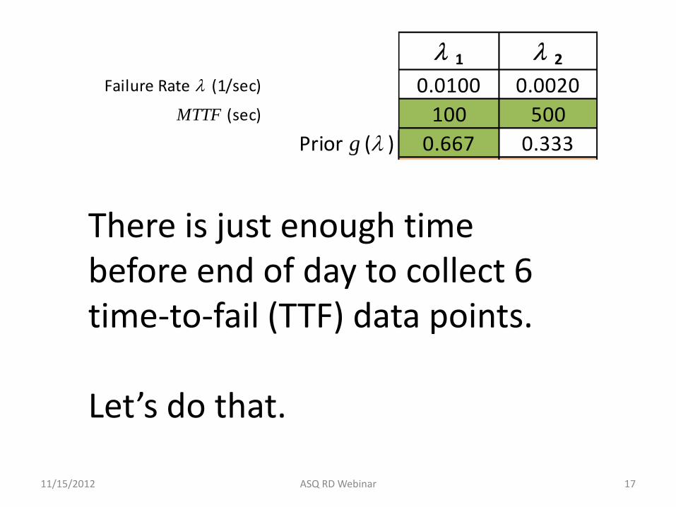
There is just enough time before end of day to collect 6 time-to-fail (TTF) data points. Let’s do that.
11/15/2012 ASQ RD Webinar 17
l KOtG l 1 l 2
Failure Rate l (1/sec) 0.0022 0.0100 0.0020
MTTF (sec) 450 100 500
Prior g (l ) 0.667 0.333
Posterior g (l | t i ) 0.204 0.796Prior*Likelihood 3.66E-21 1.43E-20
Likelihood P f (t i ) 5.49E-21 1.43E-18
average {t i } = 317
i TTF data t i (sec) f 1(t i ) f 2(t i )
1 133 2.65E-03 1.53E-03
2 888 1.39E-06 3.39E-04
3 619 2.05E-05 5.80E-04
4 8 9.23E-03 1.97E-03
5 97 3.78E-03 1.65E-03
6 157 2.08E-03 1.46E-03
11/15/2012 ASQ RD Webinar 18
l KOtG l 1 l 2
Failure Rate l (1/sec) 0.0022 0.0100 0.0020
MTTF (sec) 450 100 500
Prior g (l ) 0.667 0.333
Posterior g (l | t i ) 0.204 0.796Prior*Likelihood 3.66E-21 1.43E-20
Likelihood P f (t i ) 5.49E-21 1.43E-18
average {t i } = 317
i TTF data t i (sec) f 1(t i ) f 2(t i )
1 133 2.65E-03 1.53E-03
2 888 1.39E-06 3.39E-04
3 619 2.05E-05 5.80E-04
4 8 9.23E-03 1.97E-03
5 97 3.78E-03 1.65E-03
6 157 2.08E-03 1.46E-03
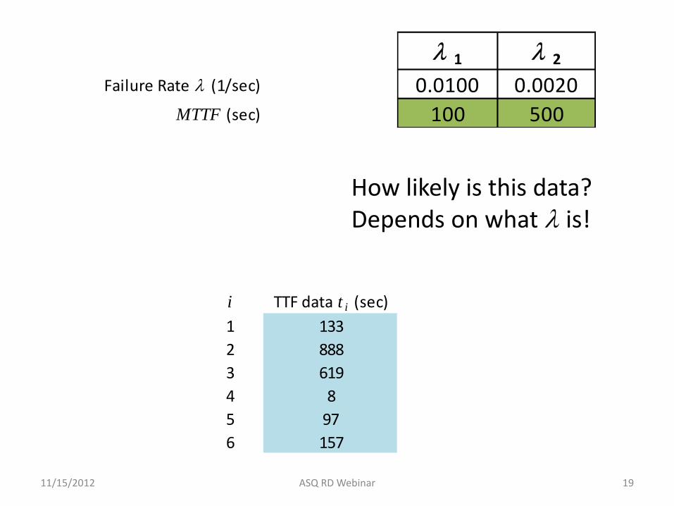
How likely is this data? Depends on what l is!
11/15/2012 ASQ RD Webinar 19

l KOtG l 1 l 2
Failure Rate l (1/sec) 0.0022 0.0100 0.0020
MTTF (sec) 450 100 500
Prior g (l ) 0.667 0.333
Posterior g (l | t i ) 0.204 0.796Prior*Likelihood 3.66E-21 1.43E-20
Likelihood P f (t i ) 5.49E-21 1.43E-18
average {t i } = 317
i TTF data t i (sec) f 1(t i ) f 2(t i )
1 133 2.65E-03 1.53E-03
2 888 1.39E-06 3.39E-04
3 619 2.05E-05 5.80E-04
4 8 9.23E-03 1.97E-03
5 97 3.78E-03 1.65E-03
6 157 2.08E-03 1.46E-03
11/15/2012 ASQ RD Webinar 20
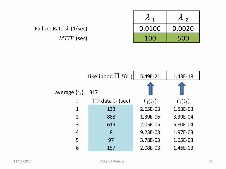
l KOtG l 1 l 2
Failure Rate l (1/sec) 0.0022 0.0100 0.0020
MTTF (sec) 450 100 500
Prior g (l ) 0.667 0.333
Posterior g (l | t i ) 0.204 0.796Prior*Likelihood 3.66E-21 1.43E-20
Likelihood P f (t i ) 5.49E-21 1.43E-18
average {t i } = 317
i TTF data t i (sec) f 1(t i ) f 2(t i )
1 133 2.65E-03 1.53E-03
2 888 1.39E-06 3.39E-04
3 619 2.05E-05 5.80E-04
4 8 9.23E-03 1.97E-03
5 97 3.78E-03 1.65E-03
6 157 2.08E-03 1.46E-03
11/15/2012 ASQ RD Webinar 21

l KOtG l 1 l 2
Failure Rate l (1/sec) 0.0022 0.0100 0.0020
MTTF (sec) 450 100 500
Prior g (l ) 0.667 0.333
Posterior g (l | t i ) 0.204 0.796Prior*Likelihood 3.66E-21 1.43E-20
Likelihood P f (t i ) 5.49E-21 1.43E-18
average {t i } = 317
i TTF data t i (sec) f 1(t i ) f 2(t i )
1 133 2.65E-03 1.53E-03
2 888 1.39E-06 3.39E-04
3 619 2.05E-05 5.80E-04
4 8 9.23E-03 1.97E-03
5 97 3.78E-03 1.65E-03
6 157 2.08E-03 1.46E-03
11/15/2012 ASQ RD Webinar 22
l KOtG l 1 l 2
Failure Rate l (1/sec) 0.0022 0.0100 0.0020
MTTF (sec) 450 100 500
Prior g (l ) 0.667 0.333
Posterior g (l | t i ) 0.204 0.796Prior*Likelihood 3.66E-21 1.43E-20
Likelihood P f (t i ) 5.49E-21 1.43E-18
average {t i } = 317
i TTF data t i (sec) f 1(t i ) f 2(t i )
1 133 2.65E-03 1.53E-03
2 888 1.39E-06 3.39E-04
3 619 2.05E-05 5.80E-04
4 8 9.23E-03 1.97E-03
5 97 3.78E-03 1.65E-03
6 157 2.08E-03 1.46E-03
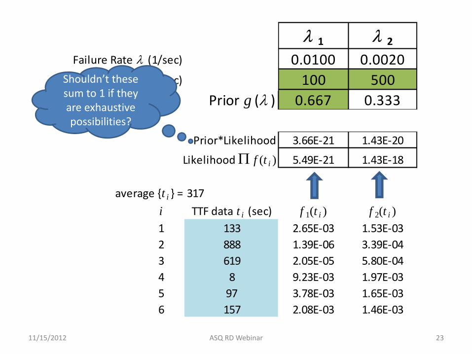
Shouldn’t these sum to 1 if they are exhaustive possibilities?
11/15/2012 ASQ RD Webinar 23

l KOtG l 1 l 2
Failure Rate l (1/sec) 0.0022 0.0100 0.0020
MTTF (sec) 450 100 500
Prior g (l ) 0.667 0.333
Posterior g (l | t i ) 0.204 0.796Prior*Likelihood 3.66E-21 1.43E-20
Likelihood P f (t i ) 5.49E-21 1.43E-18
average {t i } = 317
i TTF data t i (sec) f 1(t i ) f 2(t i )
1 133 2.65E-03 1.53E-03
2 888 1.39E-06 3.39E-04
3 619 2.05E-05 5.80E-04
4 8 9.23E-03 1.97E-03
5 97 3.78E-03 1.65E-03
6 157 2.08E-03 1.46E-03
11/15/2012 ASQ RD Webinar 24

go to the spreadsheet
11/15/2012 ASQ RD Webinar 25

Agenda
• Bayesian vs. Frequentist Comparison
• Preliminary Example
• Conjugate Priors
• Test Time Examples
• Question and Answer
11/15/2012 ASQ RD Webinar 26

Agenda
• Bayesian vs. Frequentist Comparison
• Preliminary Example
• Conjugate Priors
• Test Time Examples
• Question and Answer
11/15/2012 ASQ RD Webinar 27

Conjugate Prior
11/15/2012 ASQ RD Webinar 28

Mean lave = a/b Variance s2 = a/b2
In hierarchical Bayesian models, these hyperparameters will be represented as distributions with priors/posteriors, etc and have hyperparameters of their own
11/15/2012 ASQ RD Webinar 29

Bayesian assumptions for the gamma exponential system model
1. Failure times for the system under investigation can be adequately
modeled by the exponential distribution with constant failure rate. 2. The MTBF for the system can be regarded as chosen from a prior
distribution model that is an analytic representation of our previous information or judgments about the system's reliability. The form of this prior model is the gamma distribution (the conjugate prior for the exponential model).
The prior model is actually defined for l = 1/MTBF. 3. Our prior knowledge is used to choose the gamma parameters
a and b for the prior distribution model for l. There are a number of ways to convert prior knowledge to gamma parameters.
11/15/2012 ASQ RD Webinar 30
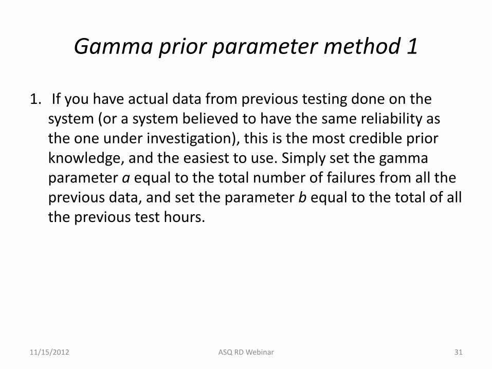
Gamma prior parameter method 1
1. If you have actual data from previous testing done on the system (or a system believed to have the same reliability as the one under investigation), this is the most credible prior knowledge, and the easiest to use. Simply set the gamma parameter a equal to the total number of failures from all the previous data, and set the parameter b equal to the total of all the previous test hours.
11/15/2012 ASQ RD Webinar 31

Gamma prior parameter method 2
2. A consensus method for determining a and b that works well is the following: Assemble a group of engineers who know the system and its sub-components well from a reliability viewpoint.
A. Have the group reach agreement on a reasonable MTBF they expect the system to have. They could each pick a number they would be willing to bet even money that the system would either meet or miss, and the average or median of these numbers would be their 50% best guess for the MTBF. Or they could just discuss even-money MTBF candidates until a consensus is reached.
B. Repeat the process again, this time reaching agreement on a low MTBF they expect the system to exceed. A "5%" value that they are "95% confident" the system will exceed (i.e., they would give 19 to 1 odds) is a good choice. Or a "10%" value might be chosen (i.e., they would give 9 to 1 odds the actual MTBF exceeds the low MTBF). Use whichever percentile choice the group prefers.
C. Call the reasonable MTBF MTBF50 and the low MTBF you are 95% confident the system will exceedMTBF05. These two numbers uniquely determine gamma parameters a and b that have percentile values at the right locations
Called the 50/95 method (or the 50/90 method if one uses MTBF10 , etc.)
11/15/2012 ASQ RD Webinar 32
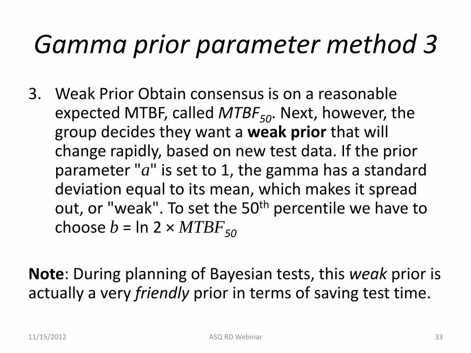
Gamma prior parameter method 3
3. Weak Prior Obtain consensus is on a reasonable expected MTBF, called MTBF50. Next, however, the group decides they want a weak prior that will change rapidly, based on new test data. If the prior parameter "a" is set to 1, the gamma has a standard deviation equal to its mean, which makes it spread out, or "weak". To set the 50th percentile we have to choose b = ln 2 × MTBF50
Note: During planning of Bayesian tests, this weak prior is actually a very friendly prior in terms of saving test time.
11/15/2012 ASQ RD Webinar 33
Comments
Many variations are possible, based on the above three methods. For example, you might have prior data from sources that you don't completely trust. Or you might question whether the data really apply to the system under investigation. You might decide to "weight" the prior data by .5, to "weaken" it. This can be implemented by setting a = .5 x the number of fails in the prior data and b = .5 times the number of test hours. That spreads out the prior distribution more, and lets it react quicker to new test data.
11/15/2012 ASQ RD Webinar 34
New data is collected …
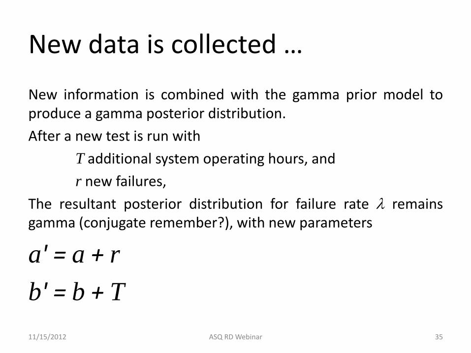
New information is combined with the gamma prior model to produce a gamma posterior distribution.
After a new test is run with
T additional system operating hours, and
r new failures,
The resultant posterior distribution for failure rate l remains gamma (conjugate remember?), with new parameters
a' = a + r
b' = b + T
11/15/2012 ASQ RD Webinar 35
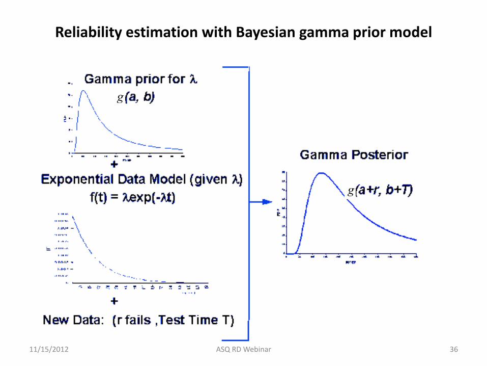
Reliability estimation with Bayesian gamma prior model
11/15/2012 ASQ RD Webinar 36
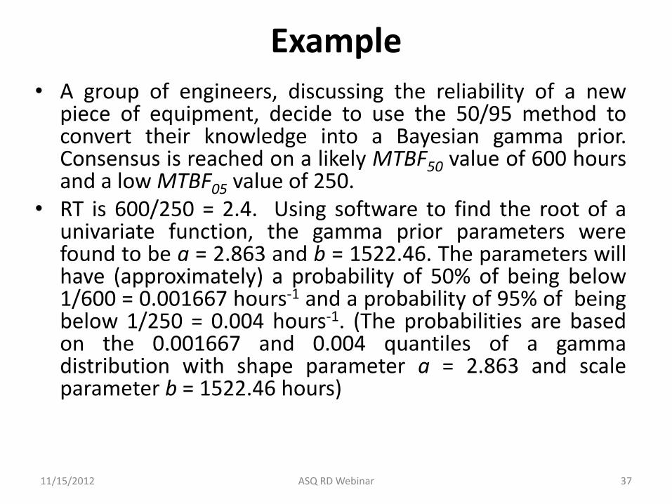
Example • A group of engineers, discussing the reliability of a new
piece of equipment, decide to use the 50/95 method to convert their knowledge into a Bayesian gamma prior. Consensus is reached on a likely MTBF50 value of 600 hours and a low MTBF05 value of 250.
• RT is 600/250 = 2.4. Using software to find the root of a univariate function, the gamma prior parameters were found to be a = 2.863 and b = 1522.46. The parameters will have (approximately) a probability of 50% of being below 1/600 = 0.001667 hours-1 and a probability of 95% of being below 1/250 = 0.004 hours-1. (The probabilities are based on the 0.001667 and 0.004 quantiles of a gamma distribution with shape parameter a = 2.863 and scale parameter b = 1522.46 hours)
11/15/2012 ASQ RD Webinar 37
Agenda
• Bayesian vs. Frequentist Comparison
• Preliminary Example
• Conjugate Priors
• Test Time Examples
• Question and Answer
11/15/2012 ASQ RD Webinar 38

Agenda
• Bayesian vs. Frequentist Comparison
• Preliminary Example
• Conjugate Priors
• Test Time Examples
• Question and Answer
11/15/2012 ASQ RD Webinar 39
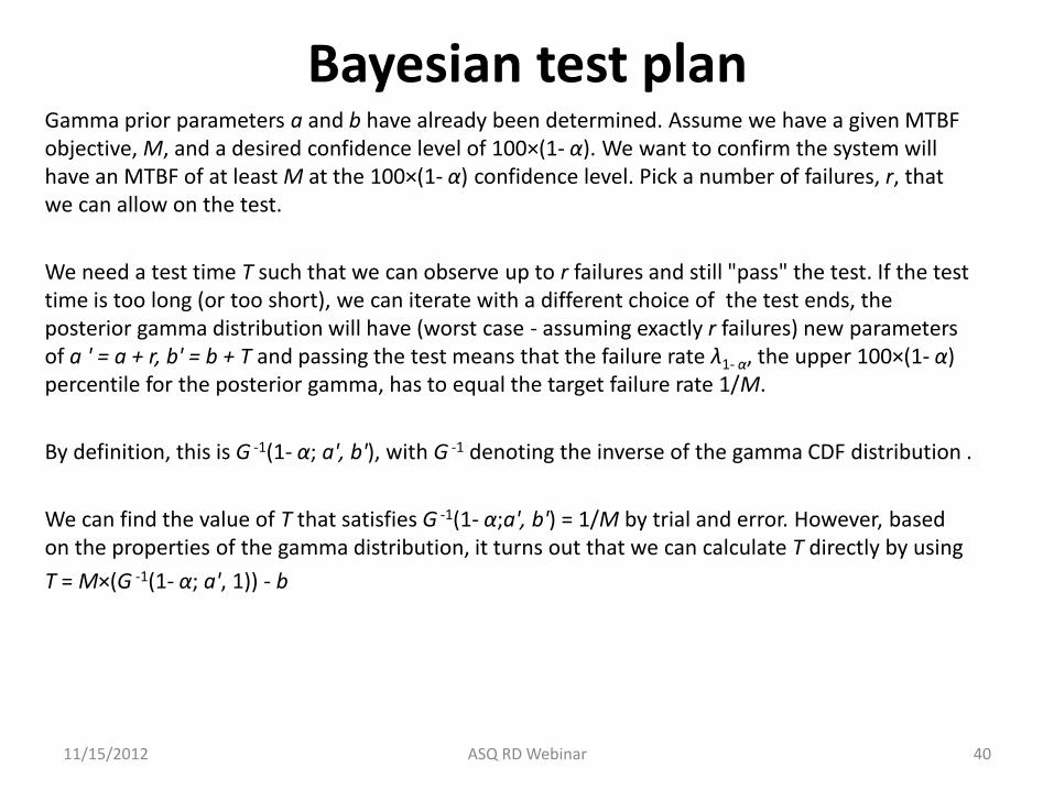
Bayesian test plan Gamma prior parameters a and b have already been determined. Assume we have a given MTBF
objective, M, and a desired confidence level of 100×(1- α). We want to confirm the system will have an MTBF of at least M at the 100×(1- α) confidence level. Pick a number of failures, r, that we can allow on the test.
We need a test time T such that we can observe up to r failures and still "pass" the test. If the test time is too long (or too short), we can iterate with a different choice of the test ends, the posterior gamma distribution will have (worst case - assuming exactly r failures) new parameters of a ' = a + r, b' = b + T and passing the test means that the failure rate λ1- α, the upper 100×(1- α) percentile for the posterior gamma, has to equal the target failure rate 1/M.
By definition, this is G -1(1- α; a', b'), with G -1 denoting the inverse of the gamma CDF distribution .
We can find the value of T that satisfies G -1(1- α;a', b') = 1/M by trial and error. However, based on the properties of the gamma distribution, it turns out that we can calculate T directly by using
T = M×(G -1(1- α; a', 1)) - b
11/15/2012 ASQ RD Webinar 40
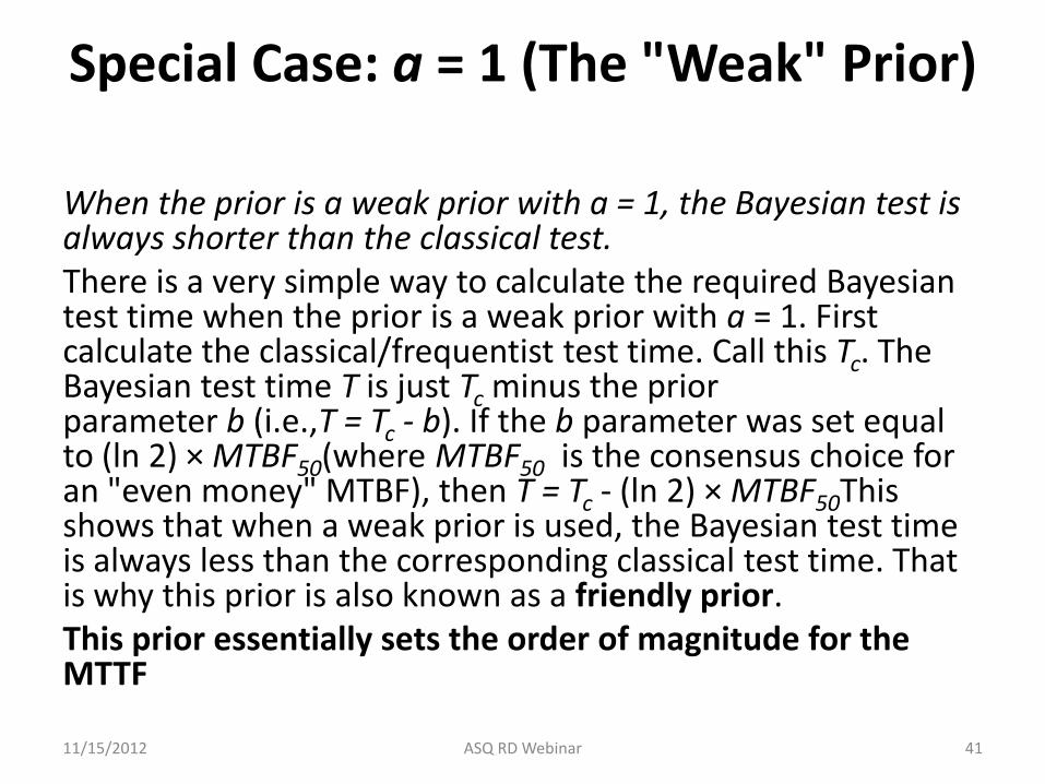
Special Case: a = 1 (The "Weak" Prior)
When the prior is a weak prior with a = 1, the Bayesian test is always shorter than the classical test. There is a very simple way to calculate the required Bayesian test time when the prior is a weak prior with a = 1. First calculate the classical/frequentist test time. Call this Tc. The Bayesian test time T is just Tc minus the prior parameter b (i.e.,T = Tc - b). If the b parameter was set equal to (ln 2) × MTBF50(where MTBF50 is the consensus choice for an "even money" MTBF), then T = Tc - (ln 2) × MTBF50This shows that when a weak prior is used, the Bayesian test time is always less than the corresponding classical test time. That is why this prior is also known as a friendly prior. This prior essentially sets the order of magnitude for the MTTF 11/15/2012 ASQ RD Webinar 41
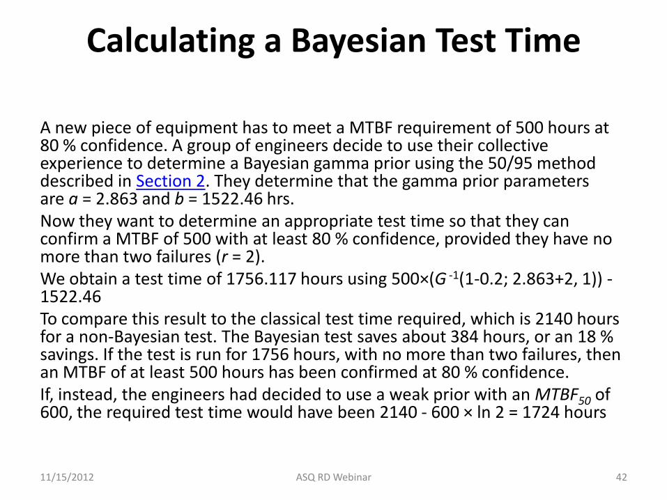
Calculating a Bayesian Test Time
A new piece of equipment has to meet a MTBF requirement of 500 hours at 80 % confidence. A group of engineers decide to use their collective experience to determine a Bayesian gamma prior using the 50/95 method described in Section 2. They determine that the gamma prior parameters are a = 2.863 and b = 1522.46 hrs. Now they want to determine an appropriate test time so that they can confirm a MTBF of 500 with at least 80 % confidence, provided they have no more than two failures (r = 2). We obtain a test time of 1756.117 hours using 500×(G -1(1-0.2; 2.863+2, 1)) - 1522.46 To compare this result to the classical test time required, which is 2140 hours for a non-Bayesian test. The Bayesian test saves about 384 hours, or an 18 % savings. If the test is run for 1756 hours, with no more than two failures, then an MTBF of at least 500 hours has been confirmed at 80 % confidence. If, instead, the engineers had decided to use a weak prior with an MTBF50 of 600, the required test time would have been 2140 - 600 × ln 2 = 1724 hours
11/15/2012 ASQ RD Webinar 42

Post-Test Analysis Example
• A system has completed a reliability test aimed at confirming a 600 hour MTBF at an 80% confidence level. Before the test, a gamma prior with a = 2, b = 1400 was agreed upon, based on testing at the vendor's location. Bayesian test planning calculations, allowing up to 2 new failures, called for a test of 1909 hours.
• When that test was run, there actually were exactly two failures. What can be said about the reliability? The posterior gamma CDF has parameters a' = 4 and b' = 3309.
11/15/2012 ASQ RD Webinar 43

What about Weibull or other non-exponential variable failure rate TTF distributions?
Conjugate priors only exist for Weibull when a subset of hyperparameters are known. MCMC and Gibbs methods exist for sampling from higher dimensional posteriors CDFs in multiple dimensions not as straightforward.
Bayesian solutions for arbitrary F(t)
0.00E+00
5.00E-03
1.00E-02
1.50E-02
2.00E-02
2.50E-02
3.00E-02
3.50E-02
0.0000 0.0020 0.0040 0.0060 0.0080
g(l, b|data)
l (1/sec)
b = 0.6
b = 0.8
b = 1.0
b = 1.2
b = 1.4
b = 1.6
11/15/2012 ASQ RD Webinar 44
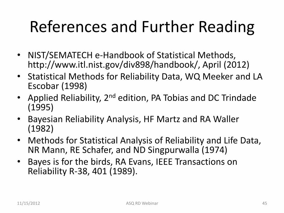
References and Further Reading
• NIST/SEMATECH e-Handbook of Statistical Methods, http://www.itl.nist.gov/div898/handbook/, April (2012)
• Statistical Methods for Reliability Data, WQ Meeker and LA Escobar (1998)
• Applied Reliability, 2nd edition, PA Tobias and DC Trindade (1995)
• Bayesian Reliability Analysis, HF Martz and RA Waller (1982)
• Methods for Statistical Analysis of Reliability and Life Data, NR Mann, RE Schafer, and ND Singpurwalla (1974)
• Bayes is for the birds, RA Evans, IEEE Transactions on Reliability R-38, 401 (1989).
11/15/2012 ASQ RD Webinar 45
Agenda
• Bayesian vs. Frequentist Comparison
• Preliminary Example
• Conjugate Priors
• Test Time Examples
• Question and Answer
11/15/2012 ASQ RD Webinar 47
Agenda
• Bayesian vs. Frequentist Comparison
• Preliminary Example
• Conjugate Priors
• Test Time Examples
• Question and Answer
11/15/2012 ASQ RD Webinar 48

Q&A
11/15/2012 ASQ RD Webinar 49