bayesian methods to overcome the winner's curse in genetic...

The Annals of Applied Statistics2011, Vol. 5, No. 1, 201–231DOI: 10.1214/10-AOAS373© Institute of Mathematical Statistics, 2011

BAYESIAN METHODS TO OVERCOME THE WINNER’SCURSE IN GENETIC STUDIES1

BY LIZHEN XU, RADU V. CRAIU2 AND LEI SUN2

University of Toronto

Parameter estimates for associated genetic variants, report ed in the initialdiscovery samples, are often grossly inflated compared to the values observedin the follow-up replication samples. This type of bias is a consequence ofthe sequential procedure in which the estimated effect of an associated ge-netic marker must first pass a stringent significance threshold. We proposea hierarchical Bayes method in which a spike-and-slab prior is used to ac-count for the possibility that the significant test result may be due to chance.We examine the robustness of the method using different priors correspond-ing to different degrees of confidence in the testing results and propose aBayesian model averaging procedure to combine estimates produced by dif-ferent models. The Bayesian estimators yield smaller variance compared tothe conditional likelihood estimator and outperform the latter in studies withlow power. We investigate the performance of the method with simulationsand applications to four real data examples.

1. Introduction. Parameter estimates such as odds ratios (OR) for an associ-ated genetic variant (e.g., SNP, Single-Nucleotide Polymorphism), reported fromthe same discovery samples that were initially used to declare statistical signifi-cance, are often grossly inflated compared to the values observed in the follow-upreplication samples [e.g., Nair, Duffin and Helms (2009)]. This type of bias is aconsequence of using the same data for both model selection and parameter es-timation, because a declared associated variant must pass a stringent significancethreshold. This phenomenon is also known as the Beavis effect [Xu (2003)] or thewinner’s curse [Zöllner and Pritchard (2007)] in the biostatistics literature.

The winner’s curse has recently gained much attention in genetic studies, be-cause it has been recognized as one of the major contributing factors to the failuresof many attempted replication studies [e.g., Ioannidis, Thomas and Daly (2009)].For example, five Nature Genetic publications in the first three months of 2009 ac-knowledged the effect of the winner’s curse [e.g., Nair, Duffin and Helms (2009)].In their recent Nature Review paper, Ioannidis, Thomas and Daly (2009) dedi-cated a section to the winner’s curse and emphasized that “the magnitude of the

Received September 2009; revised May 2010.1Supported by a research grant from the Canadian Institute of Health Research (CIHR).2Supported by grants from the Natural Sciences and Engineering Research Council of Canada

(NSERC).Key words and phrases. Association study, Bayesian model averaging, hierarchical Bayes model,

spike-and-slab prior, winner’s curse.

201

http://www.imstat.org/aoas/

http://dx.doi.org/10.1214/10-AOAS373

http://www.imstat.org

202 L. XU, R. V. CRAIU AND L. SUN

winner’s curse is inversely related to the power of the study. In typical circum-stances, for 10% power, the inflation of an additive effect could be approximately60%. . . . For small effects [anticipated for susceptibility loci associated with com-plex diseases/traits], even large meta-analyses could be grossly under-poweredand emerging associations could be considerably inflated. For rare variants, thepower can be <1%.”

Some authors [e.g., Göring, Terwilliger and Blangero (2001)] have argued thatreliable parameter estimates can be obtained only from an independent sample.However, collecting additional samples could be undesirable due to, for example,time and budget constraints as well as concerns over population heterogeneity andsampling differences. Two categories of methods were subsequently proposed tocorrect for the selection bias using the original samples only: the model-free re-sampling based methods [Sun and Bull (2005); Wu, Sun and Bull (2006); Yu et al.(2007); Jefferies (2007)] and the likelihood based methods [Zöllner and Pritchard(2007); Ghosh, Zou and Wright (2008); Zhong and Prentice (2008); Xiao andBoehnke (2009)]. Both types of approaches were shown to substantially reducethe estimation bias in relatively small samples, and comparable performances wereobserved by Faye et al. (2009). However, one caveat is that the variances of theproposed estimators in both categories are considerably higher than the originalnaïve estimator and lead to highly variable estimates of the sample size neededfor replication studies. Although the increased variability is expected, due to thebias-variance trade-off, it may be too high to provide practical design recommen-dations. For example, Figure 4 of Zöllner and Pritchard (2007) shows that the bias-adjusted sample size estimates range from ∼500 to ∼100,000 compared to theactual required sample size of 1,261 for a successful replication study (α = 10−6,power = 80%).

Motivated by the above observations and the fact that some form of prior infor-mation is often available in genetic studies, we propose here a Bayesian frameworkto further reduce the bias and decrease the variability in the estimates. In particu-lar, we focus on the OR estimates from genome-wide association studies (GWAS)via logistic regression analyses of case-control disease status, because most of thecurrent genetic mapping studies adopt the case-control GWAS design. We first de-scribe the statistical model in Section 2. We prove in Section 3 that, conditionalon statistical significance, there are no unbiased estimators for the log OR. Wepresent the Bayesian methodology in Section 4 with detailed discussions on theprior specifications and the advantages of model averaging. We assess the perfor-mance of the proposed methods in Section 5 via extensive simulation studies undera general normal model and specific genetic models. We demonstrate the utility ofour methods in Section 6 with applications to four different association studies,including a candidate gene study and three GWAS of either binary case-control orquantitative outcomes. Our concluding remarks are in Section 7.

BAYESIAN METHODS FOR WINNER’S CURSE 203

2. The statistical model. Let β refer to the true log Odds Ratio (OR), theparameter of interest, for the risk allele of an associated SNP, and Z the statistic ofthe corresponding association test. Following Ghosh, Zou and Wright (2008), weassume that Z is asymptotically normally distributed and has the form

Z = β

SE(β)∼ N

(β

SE(β),1

),

where β is the estimate for β from the logistic regression, logit(E[Y ]) = α + βX,in which the response variable Y is the affection status of a sample (0 = unaf-fected and 1 = affected by the disease of interest) and the predictor X ∈ {0,1,2}is the SNP genotype coded additively (X represents the number of copies of therisk allele). Other covariates may be also included in the model. Without loss ofgenerality, we assume that the minor allele is the risk allele and the alternative ofinterest is one-sided, that is, H0 :β = 0 vs. H1 :β > 0. The association test in thiscase is based on the Wald test, and if the null hypothesis is rejected, the standardpractice is to directly use the β from the logistic regression as the estimate for β .

The above estimation procedure is essentially the same as the familiar prac-tice of population mean estimation in the following more general statistical setup.Assuming that n i.i.d. samples, {X1, . . . ,Xn}, were collected from a normalpopulation with mean μ and variance σ 2, a significance test is first conductedfor H0 :μ = 0 vs. H1 :μ > 0 based on the statistic, Tn = X

S/√

n, which follows

N(μ

σ/√

n,1), where X and S are the sample mean and standard deviation. The

sample mean X, calculated from the same sample, is subsequently used as an esti-mate for μ, without adjusting for the fact that the null hypothesis was rejected (i.e.,Tn > c, where c is the critical value corresponding to type I error rate α) and thatestimation is performed for samples with positive findings only. Note that, in oursimplified model, although E[X] = μ, the conditional mean E[X|X > (cS/

√n)]

is strictly greater than μ, unless the power of the test is 100%. Thus, this naïveestimate, X, is upward biased. The amount of bias is inversely proportional to thepower as was first demonstrated by Göring, Terwilliger and Blangero (2001) ingenome-wide linkage analyses and later by Garner (2007) for genome-wide asso-ciation studies. The likelihood based methods proposed by Ghosh, Zou and Wright(2008) and others propose to correct for this selection bias by calculating the max-imum likelihood estimate (MLE) of μ from the correct conditional likelihood. Inthis setting,

P(X|μ,σ 2, Tn > c) =n∏

i=1

(1/√

2πσ 2) exp[−(Xi − μ)2/2σ 2]1 − �(c − μ/(σ/

√n))

,(2.1)

where � is the cumulative distribution function (c.d.f.) of the standard normaldistribution.


Although the above normal model is a conceptual one, it connects directly withthe logistic model used for case-control association studies. Specifically, β (thetrue log OR) corresponds to μ (the normal population mean), β (the naïve es-timate) corresponds to the statistic X, and SE(β) corresponds to S/

√n. In the

following development of the bias correction Bayesian methods, we choose to fo-cus on the normal model for a number of reasons. The key factor that influencesthe selection bias is the power of the association test, which depends on the non-centrality parameter, β/SE(β). In practice, β is the true log OR, but SE(β) is acomplex function of multiple components including the prevalence of the diseasein the population, the disease model (e.g., additive, dominant or others), the minorallele frequency of the SNP, the sample size and the significance threshold used[Slager and Schaid (2001)]. The normal model allows us to concisely control themain factor of interest, the power of the association test, in the simulation studies,by fixing the normal population mean (μ ↔ β , the log OR) and considering practi-cally meaningful ranges of significance threshold value, power and sample size (n),which in turn determine the normal population variance [σ , and σ/

√n ↔ SE(β)].

Moreover, this conceptual normal model also covers association analyses of quan-titative outcome, Y, for which a linear regression model is typically used, for ex-ample, E[Y ] = α + βX. In that case, the population mean μ in the conceptualnormal model represents the regression coefficient β . In Section 6 we show howour Bayesian methods built upon this conceptual normal model can be appliedto published association studies for which only the OR (or the regression coeffi-cient), the association p-value, the sample size and the significance threshold wereavailable.

In the following, we first show that there are no unbiased estimators for thepopulation mean conditionally on the significance of the corresponding hypothesistest. We then proceed with the development of a catalogue of Bayesian estimatorsand the evaluation of their performance via simulation and application studies.

3. Lack of unbiased estimators for μ. Ghosh, Zou and Wright (2008) andother authors have demonstrated that the MLE from the correct conditional likeli-hood could substantially reduce the bias. However, they also observed via simula-tion studies that the conditional MLE tends to over-correct for large μ and under-correct for small μ. Stallard, Todd and Whitehead (2008) showed that there is noconditional unbiased estimators for the effect of treatment A from a sample thatwas first used to select treatment A over B, that is, conditioning on the fact thatthe sample effect of treatment A was larger than that of treatment B. Althoughprevious authors [Zhong and Prentice (2008); Bowden and Dudbridge (2009)] dis-cussed that a similar argument can be used in the case considered here, below weprovide a formal proof to show that there are no unbiased conditional estimatorsfor the population mean μ even when the population variance σ 2 is known.

Because Tn is a sufficient statistic for μ when σ is known, the completenessof the normal family of distributions implies that we can restrict the search for


unbiased estimators of μ

σ/√

nto functions of Tn. Now suppose that some function

h(Tn) is an unbiased estimator of μ

σ/√

nconditional on the statistical significance,

that is, Tn > c. Let g(Tn) = {Tn − h(Tn)}, then

E[g(Tn)|Tn > c] = E[Tn|Tn > c] − E[h(Tn)|Tn > c]

=∫ ∞c

Tn

φ(Tn − μ/(σ/√

n))

1 − �(c − μ/(σ/√

n))d(Tn) − μ

σ/√

n

= 1

B

∫ ∞c−μ/(σ/

√n)

(z + μ

σ/√

n

)φ(z) dz − μ

σ/√

n

= 1

B

[∫ ∞c−μ/(σ/

√n)

z · e−z2/2 dz + B · μ

σ/√

n

]− μ

σ/√

n

= 1

B

[φ

(c − μ

σ/√

n

)+ B · μ

σ/√

n

]− μ

σ/√

n

= φ(c − μ/(σ/√

n))

1 − �(c − μ/(σ/√

n)),

where B = 1 − �(c − μ

σ/√

n).

Thus, we have∫ ∞c

g(Tn)φ(Tn − μ/(σ/

√n))

1 − �(c − μ/(σ/√

n))dTn = φ(c − μ/(σ/

√n))

1 − �(c − μ/(σ/√

n)),(3.1)

which implies ∫ ∞c

g(Tn)φ

(Tn − μ

σ/√

n

)dTn = φ

(c − μ

σ/√

n

).(3.2)

Now, let δc(y) be the Dirac delta function defined for y ≥ c such that it isequal to 0 for all y greater than c and

∫ εc δc(y) dy = 1 for all ε > 0. It is easy

to see that a solution to equation (3.2) is g(Tn) = δc(Tn). By the completeness ofthe normal distribution, the solution g(Tn) · 1{Tn>c} is unique almost everywhere.Thus, h(Tn) · 1{Tn>c} = Tn · 1{Tn>c} holds almost everywhere. Hence, Tn is also anunbiased estimator for μ

σ/√

n. However, Tn · 1{Tn>c} has an upward bias equal to

φ(c−μ/(σ/√

n))

1−�(c−μ/(σ/√

n)). Therefore, we conclude that there are no unbiased estimators of

μ

σ/√

nand hence no unbiased estimators of μ.

4. Bayesian bias correction.

4.1. Prior specification. The possible available prior information for genome-wide association studies (GWAS) is diverse due to, for example, results from pre-vious genome-wide linkage analyses or candidate studies, or biological evidenceon the SNPs. One common theme, however, is the anticipated low power of the


GWAS and the well-acknowledged fact that an apparent significantly associatedSNP could be a false positive [Ioannidis, Thomas and Daly (2009)]. Thus, the per-formance of the proposed Bayesian methods is assessed in this context, althoughthe practical implementation of the methods could be study specific depending onthe type of the available prior.

The Bayesian paradigm allows us to incorporate in our model the prior beliefthat the significance of the effect observed may be due to chance. Mathematically,this belief can be modeled using a spike-and-slab prior which is essentially a mix-ture between a discrete probability with mass at zero and a continuous density f

with support on the positive real line

p(μ|ξ) = ξδ{0}(μ) + (1 − ξ)f (μ),

where ξ is either constant or a hyperparameter in the model.The spike-and-slab priors have a long history in the Bayesian literature on

variable selection and shrinkage estimation, for example, Box and Meyer (1986),Mitchell and Beauchamp (1988), George and McCulloch (1993), Chipman (1996),Clyde, DeSimone and Parmigiani (1996), Geweke (1996), and Kuo and Mallick(1998). A recent theoretical study by Ishwaran and Rao (2005) discusses the simi-larities between Bayesian procedures using the spike-and-slab priors and frequen-tist procedures.

We treat ξ as a hyperparameter with a Beta distribution, ξ ∼ Beta(a, b). Theparameters a, b reflect our degree of prior belief in μ = 0 (false positive) ver-sus μ > 0 (true positive). If we set a = b = 1, then p(ξ |a = 1, b = 1) is theUniform(0,1) density, which implies that we do not favor, a priori, any regionof (0,1). This could be considered the “noninformative” prior for ξ . The choicea = 2/3 and b = 2/3 corresponds to our belief in two extreme outcomes: ξ iseither close to 0 (believing in true positive, μ > 0) or close to 1 (believing in falsepositive, μ = 0). Smaller values for a and larger values for b, say, a = 0.5 andb = 8, lead to a higher prior confidence that the signal is real. Similarly, largervalues for a and smaller values for b, say, a = 8 and b = 0.5, correspond to priorskepticism regarding the observed association between the significant SNP and thetrait of interest. Figure 1 shows the Beta distribution of ξ for different values of a

and b.Although we focus on Beta(0.5, 8), and Beta(8, 0.5) in evaluating the perfor-

mance of the proposed Bayesian methods, we conducted additional simulations tostudy the model’s robustness to the choice of priors. Simulation results included inthe supplementary material indicate that other values for a and b [e.g., Beta(0.5,16) or Beta(4, 0.5)] that preserve the L-shaped or the “inverse” L-shaped density,as seen in Figure 1, produce very similar inferences.

In the existing likelihood approaches the sample variance, S2, is typically usedto estimate σ 2 [Ghosh, Zou and Wright (2008)]. Although the variance estimatorhas relatively high precision in large samples, it could be subject to the selection


FIG. 1. Density of the prior Beta(a, b) for ξ with different choices of a and b.

bias in small samples [Faye et al. (2009)]. Therefore, we adopt an empirical Bayesprior for σ 2 in which the hyperparameters of the inverse gamma distribution, α1and α2, are chosen so that the a priori mean of σ 2 is equal to S2, the samplevariance, but the prior variance of σ 2 is equal to 200. We note that additionalsimulations with more certainty about σ 2 (prior variance of σ 2 as small as 10) orless certainty (as large as 1000) produce very similar results.

We use Uniform(0,A) to specify f (μ), the density function for the continuouscomponent of the prior for μ, the log OR, where A represents the upper boundof log OR. However, in this parametrization the estimator is very sensitive to thechoice of A. To show this, let Z be the latent mixture indicator so that Z = 0 if thesignificant SNP is a false positive (μ = 0) and Z = 1 for a true positive (μ > 0). Itis not difficult to see that

Z| �X,ξ,μ,σ 2 =

⎧⎪⎪⎨⎪⎪⎩

0, with probabilityp0

p0 + p1,


p0 + p1,

where �X = {X1, . . . ,Xn} and

p0 = ξ

1 − �(c),

p1 = 1

A× (1 − ξ) exp{−(1/(2σ 2))(nμ2 − 2μ

∑ni=1 Xi)}

1 − �(c − μ/(σ/√

n)).

Thus, depending on the value of A, p1 can be made arbitrarily small regardlessof the data available. This can influence dramatically (even for A = 2) the perfor-mance of the computational algorithm used to obtain the posterior distribution of


interest (described in Section 4.3). One simple method to circumvent this prob-lem is to use the reparametrization θ = μ/A which dissolves the influence of A

on p1. Therefore, the proposed Bayesian method has the following hierarchicalprior structure:

p(θ |ξ) = ξg0(θ) + (1 − ξ)g1(θ),(4.1)

ξ ∼ Beta(a, b),

σ 2 ∼ Inv-Gamma(α1, α2),

where α1 = S4/200 + 2, and α2 = S6/200 + S2, S is the sample standard devia-tion, g0(θ) = δ{0}(θ) and g1(θ) is the density of Uniform(0, 1).

In the actual implementation, we use A = 2 to reflect the known maximumlog OR of SNPs identified for complex diseases and traits. For example, the trulyassociated SNP in the well-known major histocompatibility complex (MHC) re-gion has perhaps the highest genetic effect observed to date, with a log OR oflog(5.49) = 1.7 [WTCCC (2007)]. We note that additional simulations showedthat, as long as the reparametrization θ = μ/A is used, results remain largelythe same for higher upper bounds (e.g., A = 6 corresponding to a maximumOR ≈ 400). Applications in Section 6 also demonstrate the robustness of the modelwhen it was applied not only to case-control data but also to an association studyof a quantitative outcome.

4.2. Posterior distribution. The joint prior distribution for (θ, ξ) is

p(θ, ξ) = p(θ |ξ)p(ξ)(4.2)

= ξg0(θ)ξa−1(1 − ξ)b−1 + (1 − ξ)g1(θ)ξa−1(1 − ξ)b−1.

Conditional on Z, the sampling distribution is

P( �X|θ, σ 2,Z,Tn > c)

∝ (1/σ)n(

exp{−∑ni=1 X2

i /(2σ 2)}1 − �(c)

)1−Z

×(

exp{−∑ni=1 (Xi − 2θ)2/(2σ 2)}

1 − �(c − 2θ/(σ/√

n))

)Z

.

If Z were observed, the posterior distribution for the vector (θ, ξ, σ 2) would be

p(θ, ξ, σ 2| �X,Z,Tn > c)

∝ p( �X,Z|θ, σ 2, Tn > c)p(θ |ξ)p(ξ)p(σ 2)

∝ (1/σ)n(

exp{−∑ni=1 X2

i /(2σ 2)}ξ1 − �(c)

)1−Z

(4.3)


×(

exp{−∑ni=1 (Xi − 2θ)2/(2σ 2)}(1 − ξ)

1 − �(c − 2θ/(σ/√

n))

)Z

× ξa−1(1 − ξ)b−1(

1

σ 2

)α1+1

exp{−α2/σ2}

for θ, ξ ∈ [0,1], σ > 0 (detailed derivation provided in the Supplementary mater-ial). We note that the posterior distribution specified in equation (4.3) depends onthe data only through the sufficient statistics for (μ,σ 2), Dn = (

∑Xi,

∑X2

i ). Thisis particularly useful in practice when the original sample-specific data �X are notavailable, but the sufficient statistics are provided or could be inferred from typi-cally reported quantities such as the sample size, the observed OR and associationp-value, and the significance threshold used.

4.3. Sampling from the posterior distribution. The latent variable Z is unob-servable in practice, so equation (4.3) cannot be used directly to study the char-acteristics of the posterior distribution, π(θ, ξ, σ 2) = p(θ, ξ, σ 2|Dn,Tn > c). Thetraditional approach in this type of situation is to use Markov chain Monte Carlo(MCMC) techniques to sample from π . The posterior distribution has a mixtureform for which the Data Augmentation algorithm of Tanner and Wong (1987) hasbeen proven extremely efficient [see also van Dyk and Meng (2001)]. The algo-rithm relies on sampling alternatively from the distribution of Z|Dn, θ, ξ, σ 2 andθ, ξ, σ 2|Z,Dn. More precisely, at iteration t we carry out the following steps:

Step 1. Sample Zt ∈ {0,1} given ξt−1, θt−1 and σ 2t−1 from the conditional dis-

tribution

Zt |ξt−1, θt−1, σ2t−1 =

⎧⎪⎪⎨⎪⎪⎩


p0 + p1,


p0 + p1,

where

p0 = ξt−1

1 − �(c),

p1 = (1 − ξt−1) exp{−(1/(2σ 2t−1))(4nθ2

t−1 − 4θt−1∑n

i=1 Xi)}1 − �(c − 2θt−1/(σt−1/

√n))

.

Step 2. (i) If Zt = 0, sample

ξt ∼ Beta(a + 1, b),

σ 2t ∼ p(σ 2|Dn) ∝

(1

σ 2

)n/2+α1+1

exp{− 1

σ 2

(α2 +

∑ni=1 X2

i

2

)},

which is the inverse gamma distribution with shape parameter equal to n2 +α1, and

scale parameter equal to α2 +∑n

i=1 X2i

2 . We also set μt = θt = 0.


(ii) If Zt = 1, sample

ξt ∼ Beta(a, b + 1),

θt ∼ p(θ |Dn,σt−1) ∝ exp{−2nθ2/σ 2t−1 − 2θ

∑ni=1 Xi/σ

2t−1}

1 − �(c − 2θ/(σt−1/√

n))1(0,1)(θ),

σ 2t ∼ p(σ 2|(Dn, ξt , θt ) ∝ exp{−1/(2σ 2)(

∑ni=1 X2

i + 4nθ2t − 4θt

∑ni=1 Xi)}

(1 − �(c − 2θt/

√σ 2/n))

× (σ 2)n/2+α1+1 exp{−α2/σ2}.

The sampling of θt and σ 2t at step 2(ii) cannot be carried out directly, so we apply a

Metropolis–Hasting algorithm [Metropolis et al. (1953)]. We use 20,000 iterationsto obtain 15,000 posterior samples, discarding the first 5000 “burn-in” samples.The sample mean of the above 15,000 posterior samples, θ , is used to estimate theposterior mean E[μ|Dn,Tn > c]. That is, μB = 2θ , where the factor 2 is due to theinitial reparametrization θ = μ/A and A = 2. (Additional simulations presented inthe Supplementary material show that running the chain longer or discarding more“burn-in” samples provide similar results.)

4.4. Bayesian Model Averaging (BMA). The Bayesian model averaging(BMA) is a coherent and conceptually simple method devised to take into ac-count the model uncertainty [see Hoeting et al. (1999) and references therein]. Forthe problem discussed here, the uncertainty is related to our lack of informationregarding the power of the test performed in the first stage. If we knew, say, thatthe power of the test is high, then we would be more confident that the signal de-tected is a true signal and this would be reflected in our choice of the prior. In theabsence of such information, one could adopt the BMA methodology to increasethe robustness of the Bayesian estimator.

In the BMA paradigm, assume that � is the quantity of inferential interest forwhich a number of candidate models, say, M1, . . . ,MK , are available. Given theprior probability for each candidate model, p(Mi),1 ≤ i ≤ K , the traditional BMAmethod assigns the posterior distribution given data D for �

p(�|D) =K∑

k=1

p(�|Mk,D)p(Mk|D),(4.4)

where

p(Mk|D) = p(D|Mk)p(Mk)∑Kl=1 p(D|Ml)p(Ml)

and

p(D|Mk) =∫

p(D|θk,Mk)p(θk|Mk)dθk.


In our setting, K = 2 because only two models are considered. Let M1 be themodel with prior p(ξ) = Beta(8,0.5) (a priori favors the belief that the initialdiscovery is a false positive) and M2 for p(ξ) = Beta(0.5,8) (a priori favors thebelief that the initial discovery is a true positive). To specify the values for p(M1)

and p(M2), we utilize the threshold value c in the following fashion, p(M1) =e(−c/2) and p(M2) = 1 − e(−c/2). Thus, our prior belief in model M1 (with higherdensity for false positive) decreases as the testing threshold value increases at anexponential rate. The posterior probabilities for the two models can be derived as

p(Mi |Dn) = p(Dn|Mi)p(Mi)

p(Dn|M1)p(M1) + p(Dn|M2)p(M2), i = 1,2.

Thus,

p(M1|Dn)

p(M2|Dn)= p(Dn|M1)

p(Dn|M2)· e(−c/2)

(1 − e(−c/2)).(4.5)

The direct computation, however, is difficult because the integral

p(Dn|M) =∫ ∫

(μ,ξ,σ 2)p(Dn|μ, ξ, σ 2,M)p(μ|ξ,M)p(ξ |M)p(σ 2|M)dμdξ

cannot be calculated in a closed form. Note that

p(μ, ξ, σ 2|Dn,M) = p(Dn|M,μ, ξ, σ 2)p(μ|ξ,M)p(ξ |M)p(σ 2|M)

p(Dn|M),(4.6)

thus p(Dn|M) can be viewed as the normalizing constant of the posterior distribu-tion p(μ, ξ, σ 2|Dn,M). Therefore, the first ratio in (4.5) is a ratio of two normal-izing constants for two densities from which we can sample. The problem of esti-mating ratios of two normalizing constants has been discussed by, among others,Meng and Wong (1996) and Gelman and Meng (1998). We use the bridge samplingmethod proposed by Meng and Wong (1996) to compute the ratio in (4.5).

To compute (4.5), let r = p(Dn|M1)/p(Dn|M2), ω = (μ, ξ, σ 2), πi = p(μ, ξ,

σ 2|Dn,Mi) and qi(μ, ξ, σ 2) = p(Dn|Mi,μ, ξ, σ 2)p(μ|ξ,Mi)p(ξ |Mi)p(σ 2|Mi),

for 1 ≤ i ≤ 2. Given m = 10,000 samples {(μi1, ξi1, σ2i1), . . . , (μini

, ξini, σ 2

i1)}from each density πi , we can approximate r using the iterative procedure of Mengand Wong (1996). Specifically, after starting with an initial estimate r (0), at the(t + 1)st iteration, we compute

r (t+1) = (1/m)∑m

j=1[q1(ω2j )/(s1q1(ω2j ) + s2r(t)q2(ω2j ))]

(1/m)∑m

j=1[q2(ω1j )/(s1q1(ω1j ) + s2r (t)q2(ω1j ))](4.7)

≡ (1/m)∑n2

j=1[l2j /(s1l2j + s2r(t))]

(1/m)∑m

j=1[1/(s1l1j + s2r (t))] ,

where si = 0.5, and lij = q1(ωij )

q2(ωij ), for 1 ≤ j ≤ m, 1 ≤ i ≤ 2. Note that lij needs to

be computed only once at the beginning of the algorithm. The convergent value ofr (t) is the one we choose to estimate r .


In the current setting lij is easy to compute since

lij = p(Dn|M1,μij , ξij , σ2ij )p(μij |ξij ,M1)p(ξij |M1)p(σ 2

ij |M1)

p(Dn|M2,μij , ξij , σ2ij )p(μij |ξij ,M2)p(ξij |M2)p(σ 2

ij |M2)

= p(ξij |M1)

p(ξij |M2)= ξ7.5

ij (1 − ξij )−7.5.

From equations (4.4) and (4.5), we obtain the BMA estimator of μ,

μBMA = re(−c/2)

re(−c/2) + 1 − e(−c/2)μ1 + 1 − e(−c/2)

re(−c/2) + 1 − e(−c/2)μ2,(4.8)

where μ1 and μ2 are the posterior means of μ obtained under models M1 and M2,respectively.

5. Simulation study. We carried out two sets of simulations to examine theperformances of the Bayesian methods and compared the results with those fromthe likelihood-based estimators of Ghosh, Zou and Wright (2008). The first set ofsimulations used data generated from the normal model that was used to outlineand develop the Bayesian methods, and the second set used data simulated from acase-control genetic model. The nine estimators examined are as follows:

N: The naïve estimator (X, the unconditional MLE).MLE: The conditional MLE estimator based on equation (2.1), that is the β1

estimator in Ghosh, Zou and Wright (2008).NMLE: The mean of the Normalized Conditional Likelihood estimator, that is,

the β2 estimator of Ghosh, Zou and Wright (2008).Ghosh: The average estimator of MLE and NMLE, that is, the β3 estimator rec-

ommended by Ghosh, Zou and Wright (2008).B.L: The Bayesian estimator based on equation (4.3) when the prior for ξ is

Beta(8,0.5) (the prior belief is low power of the initial discovery study).B.H: The Bayesian estimator based on equation (4.3) when the prior for ξ is

Beta(0.5,8) (the prior belief is high power of the initial discovery study).B.BMA: The BMA estimator obtained by averaging the B.L and B.H models,

based on equation (4.8).B.M: The Bayesian estimator based on equation (4.3) when the prior for ξ is

Beta(2/3,2/3) (the prior belief is either low or high power).B.Unif: The Bayesian estimator based on equation (4.3) when the prior for ξ is

Uniform(0,1) (the “noninformative” prior).

Whenever an obtained estimate was negative, it was truncated to be zero followingthe standard practice of interpreting the “flip–flop” phenomenon occurring at thesame SNP in the same population [Lin et al. (2007)]. That is, a SNP is found tobe associated with the disease of interest in two independent studies, but the riskallele is reversed (i.e., the allele that increases the risk in one study is the protectiveallele that decreases the risk in another study).


5.1. Simulation set 1—normal model. We considered a factorial design inwhich the factors are the power of the association test, the type 1 error rate and thesample size. The power levels are {5%,10%,20%, 50%,99%}, of which 99% al-lows us to investigate the asymptotic behavior of the methods while 20% or lowerreflect the low power anticipated for genome-wide association studies (GWAS).The type 1 error rates, α, are {0.05,10−4,10−6}, of which 0.05 is the typical choicefor a single SNP study, while the other two are suitable for high-throughput GWASdepending on the density of the SNPs being genotyped. The corresponding thresh-old values for the test statistics, c, are {1.645,3.719,4.753}. The true populationmean is fixed at μ = 0.095 = log(1.1), and the sample size ranges from n = 100 toover 10,000 depending on the combination of α and power. The values of the theseparameters then uniquely determine the corresponding population variance, σ 2.The details of each simulation scenario are shown in Table 1.

Under each simulation scenario, we began by generating 200 significant datasets, that is, Xi ∼ N(μ,σ 2), i = 1, . . . , n, such that the value of the test statistic,Tn = X

S/√

n, is greater than c. We then computed the nine estimates, N, MLE,

NMLE, Ghosh, B.L, B.H, B.BMA, B.M and B.Unif, for each significant dataset.

Figure 2 provides detailed results when the type 1 error rate is 0.05 and the sim-ulating parameter values are those in row 1 of Table 1. These plots confirm that, inthe case of low power of the initial association study (e.g., 10%), the naïve estima-tor has a large upward bias. Even in the moderately powered studies (e.g., 20%),the naïve estimator could considerably overestimate the true effect size. Note thatthe two priors with opposite degrees of belief in the significance of the effect, B.Land B.H, produce quite different results. The B.L estimator conservatively shrinksthe effect and, therefore, it is more reliable in those cases when the effect is smallor zero. (See additional figures in Supplement for the case of no genetic effect,i.e., the apparent association is a false positive.) When the power of the test is rel-atively high (e.g., 50%), B.H outperforms the other estimators considered. Whileit is clear that B.L and B.H are complementing each other, B.BMA, designed tobalance between B.L and B.H, performs well in a variety of settings. The perfor-mances of the other two estimators, B.M and B.Unif, are similar to one anotherbut inferior to B.BMA. The natural implication is that putting equal prior weighton (0,1) is equivalent to putting equal weight on ξ close to zero or close to 1. Asexpected, when the power is very high (e.g., 99%) there is little bias in the naïveestimate; the other estimates also converge to the true value with B.L lagging be-hind. This is due to the strong skepticism embedded in the B.L model about thefinding.

In most of the cases, the Bayesian estimators achieve the anticipated reductionin bias as well as variance compared to the likelihood based estimators, MLE,NMLE and Ghosh. Of the three, we observed that Ghosh (i.e., the average ofMLE and NMLE) performs the best, confirming the conclusion of Ghosh, Zou and

214L

.XU

,R.V

.CR

AIU

AN

DL

.SUN

TABLE 1Simulation scenarios for the normal model

5% 10% 20% 50% 99%

α\power n σ σ/√

n n σ σ/√

n n σ σ/√

n n σ σ/√

n n σ σ/√

n

0.05 – – – 100 2.623 0.262 200 1.678 0.119 1000 1.832 0.058 5000 1.697 0.02410−4 1000 1.453 0.046 2000 1.749 0.039 3000 1.814 0.033 5000 1.812 0.026 10,000 1.577 0.01610−6 2000 1.371 0.031 4000 1.736 0.027 5000 1.723 0.024 8000 1.793 0.020 16,000 1.702 0.013

Notes: Sample size (n) and population standard error (σ ) needed to obtain the desired power at the prespecified type 1 error rate (α) when populationmean μ = 0.0953 = log(1.1).


FIG. 2. Performance of the nine estimators under the normal model with a type 1 error rate of0.05. The population mean μ = log(1.1) = 0.0953 and power ranging from 10%, 20%, 50% to 99%.Details of the simulating parameters are given in row 1 of Table 1. Each circle represents an estimate,the horizontal is the averaged estimate over 200 simulated data sets, and the long horizontal linerepresents the true value of μ. The Bias, sample Standard Deviation (SD) and Root Mean SquaredError (RMSE) are also provided for each estimator.

Wright (2008). Therefore, in what follows we focus on the comparison betweenB.BMA and Ghosh.

The advantage of B.BMA over Ghosh is especially obvious in the low powerstudies. For example, when the power of the test is 10%, the bias of Ghosh is0.196, almost twice as big as 0.092 for B.BMA. The sample standard deviation ofthe Ghosh estimate is 0.186 compared to 0.116 for the B.BMA estimate. The RootMean Squared Error (RMSE) for B.BMA is almost half that for Ghosh (0.148 vs.0.273). To formally assess the significance of the difference between Ghosh andB.BMA, we performed a matched-pair t-test based on 50 simulation runs, andwe obtained a t-statistic of −117.47 showing that the difference is significant. Asexpected, the advantage dissipates and the two perform similarly when the powerof the initial association study increases.


As discussed by Ghosh, Zou and Wright (2008) and detailed in Section 2, themain factor that influences the estimation bias is the power of the association testwhich depends on the noncentrality parameter, μ/(σ/

√n). Thus, although μ has

the interpretation of β = log OR and was fixed at log(1.1), the results are quali-tatively similar for larger OR with smaller sample size or smaller OR with largersample size, as long as the ratio, μ/(σ/

√n), and the significance threshold value,

α, stay the same.Figure 3 shows the performance of the estimators when the type 1 error rate

is 10−6 and the parameter values are from row 3 of Table 1. We found that allthe bias correction estimators are showing a slight overcorrection. (Note that thescale in the y-axis differs between Figures 2 and 3.) In this setting, the results ofB.BMA and Ghosh are very similar with B.BMA having a smaller variance. Thedifference between Figures 2 and 3 is due to the fact that the significance thresholdused is drastically different, α = 0.05 for Figure 2 and α = 10−6 for Figure 3,while the power of the association study of the same SNP is kept comparable byincreasing the required sample size, n. As a result, the noncentrality parametervalues, μ/(σ/

√n), are not directly comparable between the two cases.

5.2. Simulation set 2—genetic model. Following the setup of the simulationsconducted by Ghosh, Zou and Wright (2008), we generated data for 500 casesand 500 controls from an additive genetic model with disease prevalence of 1%,minor allele frequency of 0.25, and the log OR, β , ranging from log(1.1) to log(2).The threshold value is c = 5.0, leading to the significance level α = 2.87 × 10−7.For each log OR value, we began by generating 200 significant data sets such thatthe association test statistic, β/SE(β), is greater than c, where β is the log ORestimate obtained from the logistic regression model, and SE(β) is the estimate ofthe standard error of β . Using the summary statistics, β and SE(β), the auxiliaryinformation such as the sample size (we used n = 1000) and the threshold value ofthe test, we applied the Bayesian methods by letting μ = β , and S = σ = SE(β)×√

n.Figure 4 illustrates the results for log OR values equal to {log(1.2), log(1.3),

log(1.4), log(1.8)}, corresponding to the power of detecting the associated SNP inthe range {0.345%, 4.515%, 21.897%, 99.5%}. (Results for other log OR valuesare qualitatively similar.) The results obtained from the simulated genetic modelsconfirm that the B.BMA has a smaller RMSE than Ghosh when the power of theassociation test is low. Although the variance reduction on the log OR scale issmall, the implication on study design is practically important. Figure 5 shows thesample size estimation for a replication study with 80% power at the 0.05 signifi-cance level using the naïve log OR estimate, the Ghosh estimate and the B.BMAestimate obtained from the original discovery samples, as reported in Figure 4.Results show that the standard error in sample size estimation based on Ghosh isalmost twice as big as that based on B.BMA when the power of the original as-sociation study is low (e.g., 20% or lower). In the low power case, we also note


FIG. 3. Performance of the nine estimators under the normal model with a type 1 error rate of10−6. The population mean μ = log(1.1) = 0.0953 and power ranging from 5%, 20%, 50% to 99%.Details of the simulating parameters are given in row 3 of Table 1. Each circle represents an estimate,the horizontal bar is the averaged estimate over 200 simulated data sets, and the long horizontal linerepresents the true value of μ. The Bias, sample Standard Deviation (SD) and Root Mean SquaredError (RMSE) are also provided for each estimator.

that the sample size predicted based on N, the naïve estimate, is never sufficient.For example, for a SNP with log(OR) of log(1.2), the naïve sample size estimatecenters around 222 with a maximum predicted size of 247, while the true expectedrequired sample size is 1170. Although both Ghosh and B.BMA overestimate thenecessary sample size for replication due to the overcorrection of effect size, webelieve that a conservative sample size estimate is practically useful because itguards against sampling variation.

We also examined different effect levels when the type I error level is equal to0.05 or 0.001, and we drew similar conclusions based on the results reported inSupplement. The additional simulation studies also include a null case where theapparent discovery is a false positive. In that case, B.BMA outperforms Ghosh,but B.L performs the best, as expected.


FIG. 4. Performance of the nine estimators under an additive genetic model with a type 1 errorrate of α = 2.87 × 10−7(c = 5). The sample size is 1000 (500 cases and 500 controls), the minorallele frequency of the causal SNP is 0.25. The effect of the SNP on the log OR scale ranging fromμ = β = log(1.2), log(1.3), log(1.4) to log(1.8) corresponding to power <1%, ≈5%, ≈20% and>95% to detect the association. Each circle represents an estimate, the horizontal bar is the averageestimate over 200 simulated data sets, and the long horizontal line represents the true value of μ.The Bias, sample Standard Deviation (SD) and Root Mean Squared Error (RMSE) are also providedfor each estimator.

6. Application study. We applied the proposed Bayesian estimation meth-ods to four data sets of which one is a candidate gene study and the other threeare genome-wide association studies (GWAS) of either binary or quantitative out-comes. Specifically, the four studies are as follows:

(I) the candidate gene association study of Lymphoma by Wang et al. (2006),(II) the GWAS of type 1 diabetes (T1D) by WTCCC (2007),

(III) the GWAS of psoriasis by Nair, Duffin and Helms (2009),(IV) the GWAS of complications of T1D by Paterson et al. (2010).

The Lymphoma and WTCCC T1D data sets were chosen because they were pre-viously analyzed by Ghosh, Zou and Wright (2008) via the likelihood-based ap-


FIG. 5. Performance of sample size estimation for replication studies under an additive geneticmodel. The initial discovery samples are the same as those in Figure 4. The replication sample size iscalculated assuming a type 1 error rate of 0.05 and power of 80%, and it is calculated based on theestimate of the log OR by N, the naïve estimation method, Ghosh, the likelihood method, or B.BMA,the Bayesian method applied to the simulated significant discovery samples. Each circle representsan estimate, the horizontal bar is the average estimate over 200 simulated data sets, and the longhorizontal line represents the true expected required sample size.

proach, and the other two studies were chosen because the genetic effect estimatesfrom independent replication samples were reported by the study authors. In ad-dition, the T1D complication data set allows us to demonstrate that the proposedmethods can be easily and robustly applied to association studies of quantitativeoutcomes.

In each case, the results are summarized in a table containing the original re-ported genetic effect (i.e., the naïve estimate, N), the five different Bayesian esti-mators, B.L, B.H, B.BMA, B.Unif and B.M, and three likelihood methods, MLE,NMLE and Ghosh, as described in Section 5. The estimates produced by eachmethod are compared with the estimates obtained from the independent replica-


tion samples reported in the literature. We note that the anticipated power foreach study differs due to the apparent differences in study design [e.g., higherpower for the candidate gene study of Wang et al. (2006) compared to the GWAS],the sample size [e.g., higher power for the GWAS of T1D by WTCCC (2007)with n ≈ 5000 compared to the GWAS of T1D complication by Paterson et al.(2010) with n = 667], and the prior knowledge of a SNP (e.g., higher power forrs12191877 from chromosome 6 in the well-known MHC region that is stronglyassociated with Psoriasis compared to other novel SNPs). However, we report es-timates from all five Bayesian estimators for a more complete comparison. Theestimate from the replication samples serves as the benchmark, but the value itselfshould not be viewed as the true parameter value because of the sampling vari-ation and the potential subpopulation and ascertainment differences between theoriginal discovery and the follow-up replication studies.

We also report the corresponding confidence interval (CI) or the highest poste-rior density region/interval (HpdI), but it should be noted that the statistical inter-pretations of CI and HpdI are different and, therefore, these regions are not directlycomparable. Although the HpdI with posterior mass 1 − η may be estimated usingsamples from the posterior under model M1 for B.L or M2 for B.H, there is nodirect way to construct a HPD region for B.BMA, the model averaging estimatorfor the two models. However, a credible interval (CrdI) can be constructed usingthe normal approximation based on the model averaging estimator and its vari-ance estimate [see equation (7) in Viallefont, Raftery and Richardson (2001)]. Forthe likelihood-based methods, we construct the CI following the method proposedby Ghosh, Zou and Wright (2008) that was shown to outperform the standard CIprocedure. Specifically, the Ghosh 1 − η CI is the interval between the η/2 and1−η/2 quantiles of the conditional density p(Tn|Tn > c). Ghosh, Zou and Wright(2008) noted that, although they proposed three competing point estimates, MLE,NMLE and Ghosh, their procedure provided only a single CI.

6.1. Application I—A candidate-gene study of lymphoma. Wang et al. (2006)performed a candidate gene study of Lymphoma using a total of 48 SNPs geno-typed on 318 cases and 766 controls, and they reported two significant SNPs us-ing a p-value threshold of α = 0.002. The naïve log OR estimate is log(1.54)for rs1800629 and log(1.40) for rs909253, however, the follow-up estimates ob-tained from a larger independent study are reduced considerably to log(1.29) forrs1800629 and log(1.16) for rs909253 [Rothman et al. (2006); Ghosh, Zou andWright (2008)]. For each of the two SNPs, we applied the likelihood estima-tion methods as well as the Bayesian methods, using the naïve log OR estimates,μ = β , and S = σ = SE(β) × √

n inferred from the observed association p-value[p-value = 1 −�(|β/SE(β)|)], n = 318 + 766 = 1084 and c = 2.878 correspond-ing to α = 0.002 (Table 2).

Results in Table 2 are consistent with simulation results of power 50% in Fig-ure 2. Because of the anticipated high power of a candidate gene study, both


TABLE 2Application I—the candidate gene study of Lymphoma by Wang et al. (2006)

SNPs of interest rs1800629 rs909253

Discovery samplesAssociation p-value 5.7 × 10−4 7.4 × 10−4

Reported effect 0.432 0.337

Likelihood estimatesMLE (CI) 0.116 (0.000, 0.645) 0.010 (0.000, 0.498)NMLE (CI) 0.247 (0.000, 0.645) 0.184 (0.000, 0.498)Ghosh (CI) 0.182 (0.000, 0.645) 0.097 (0.000, 0.498)

Bayesian estimatesB.L (HpdI) 0.005 (0.000, 0.013) 0.004 (0.000, 0.005)B.H (HpdI) 0.196 (0.000, 0.508) 0.142 (0.000, 0.382)B.BMA (CrdI) 0.150 (0.000, 0.428) 0.115 (0.000, 0.324)B.Unif (HpdI) 0.068 (0.000, 0.377) 0.045 (0.000, 0.277)B.M (HpdI) 0.074 (0.000, 0.397) 0.049 (0.000, 0.281)

Follow-up samplesFollow-up estimate 0.255 0.148

Notes: The Reported Effect is naïve log OR estimate obtained from the original discovery samples(318 cases and 766 controls) of Wang et al. (2006), in which the association tests of these two SNPswere significant at the α = 0.002 level. The follow-up estimate was obtained from a larger pooledanalysis by Rothman et al. (2006). The other eight estimates were based on either the likelihoodapproach, MLE, NMLE and Ghosh, or the proposed Bayesian approach, B.L, B.H, B.BMA, B.Unifand B.M as summarized in Section 5. CI is the 95% confidence interval for the likelihood estimates,HpdI is the highest posterior density interval with posterior mass 95% and CrdI is the credible intervalfor the Bayesian estimates.

B.BMA and Ghosh overcorrect slightly with similar performance. We observethat the CrdI of B.BMA is smaller than the CI of Ghosh, although we noted be-fore that the interpretation of the two intervals is different. Results suggest thatB.H performs best among all the Bayesian methods, which is not surprising for astudy with putative high power.

6.2. Application II—A GWAS of Type 1 Diabetes. The Type 1 Diabetes (T1D)GWAS from the WTCCC included approximatively 2000 cases and 3000 controlsand the samples were genotyped on the Affymetrix 500K chip3 [WTCCC (2007)].After a set of quality control criterions (e.g., the minor allele frequency of a SNP> 5%, the genotyping missing rate < 5% and the p-value of the Hardy–WeinbergEquilibrium test > 5.7 × 10−7), the authors reported six significant loci at the5 × 10−7 level. We focused on the four SNPs analyzed by Ghosh, Zou and Wright(2008) because the replication results are available from the study of Todd et al.(2007). For each SNP of interest, we applied the proposed estimation methodsusing the reported log OR estimates obtained from the WTCCC discovery sam-


ples, β = μ, and S = σ = SE(β) × √n inferred from the observed association

p-value, and c = 4.892 corresponding to α = 5 × 10−7 (Table 3). In this applica-tion, the actual number of cases is 1963− 37 = 1926 and the number of controls is(1480 − 24)+ (1458 − 42) = 2872, where the 37, 24 and 42 samples were deleteddue to quality control issues, based on the information provided in the supplemen-tary Tables 1 and 4 of WTCCC (2007). Thus, n = 1926 + 2872 = 4798 in thisapplication.

Results in Table 3 show that if the original association result is extremein that the p-value is considerably smaller than the threshold considered (i.e.,rs17696736), then the prior influences the result only minimally. Similarly, thelikelihood-based estimates are only slightly reduced from the published estimatedlog ORs. However, the follow-up estimate is considerably lower than the bias re-duced estimates. As noted by Ghosh, Zou and Wright (2008), this suggests pos-sible heterogeneity between the discovery and replication samples. A subtle butimportant explanation for the results in the last three columns of Table 3 wherethe replicated values are larger in absolute value than the estimates produced byeach method is that the follow-up estimates here are also subject to the winner’scurse, albeit less severe, because only estimates of successfully replicated SNPswere reported.

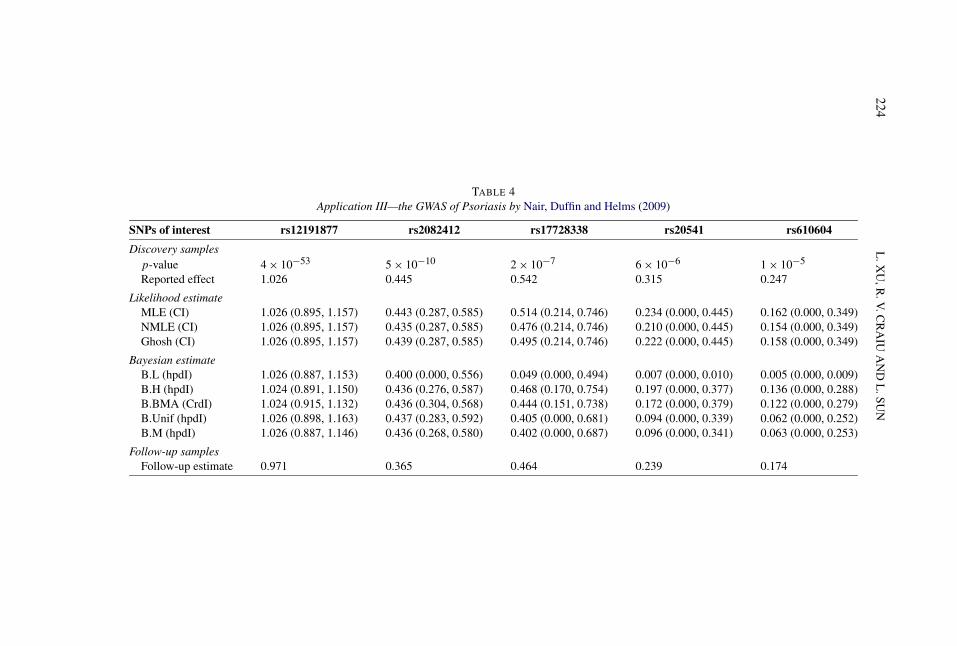
6.3. Application III—A GWAS of Psoriasis. Nair, Duffin and Helms (2009)conducted a two-stage association of Psoriasis, a chronic skin disease character-ized by circumscribed red patches covered with white scales. The first stage is aGWAS with 438,670 SNPs genotyped on 1359 cases and 1400 controls, and thesecond stage is a replication study following up on 21 promising SNPs using a setof independent 5048 cases and 5051 controls. “Owing to the winner’s curse, oddsratios estimated in the discovery sample were larger than those estimated in thefollow-up samples” [Table 2 of Nair, Duffin and Helms (2009)]. The SNP selectioncriterion was mainly based on the ranking of the GWAS p-value, roughly corre-sponding to a p-value threshold of α = 10−4. For each SNP of interest, we appliedthe estimation methods using the reported log OR estimates obtained from thediscovery samples, β = μ, and S = σ = SE(β) × √

n inferred from the observedassociation p-value, n = 1359 + 1400 = 2759 and c = 3.719 corresponding toα = 10−4 (Table 4).

When the results are as extreme as rs12191877 with p = 4 × 10−53 or asrs2082412 with p = 5 × 10−10, indicating high power at the chosen thresholdlevel, all the bias correction estimators results in little change from the publishedestimate, including B.L despite its inherent prior skepticism of a finding. For theother less significant SNPs in the table, both B.BMA and Ghosh achieve substan-tial bias reduction. In general, B.BMA has a noticeably smaller variance for lowerpower cases, which in turn can produce more reliable sample size estimates forreplication studies.

BA

YE

SIAN

ME

TH

OD

SFO

RW

INN

ER

’SC

UR

SE223

TABLE 3Application II—the GWAS of T1D by WTCCC (2007)

SNPs of interest rs17696736 rs2292239 rs12708716 rs2542151

Discovery samplesAssociation p-value 7.27 × 10−14 1.49 × 10−9 1.28 × 10−8 8.4 × 10−8

Reported effect (CI) 0.315 (0.239, 0.399) 0.262 (0.182, 0.351) −0.261 (−0.357, −0.174) 0.285 (0.182, 0.399)

Likelihood estimatesMLE (CI) 0.314 (0.224, 0.397) 0.241 (0.095, 0.346) −0.212 (−0.348, 0.000) 0.140 (0.000, 0.375)NMLE (CI) 0.310 (0.224, 0.397) 0.217 (0.095, 0.346) −0.182 (−0.348, 0.000) 0.154 (0.000, 0.375)Ghosh (CI) 0.312 (0.224, 0.397) 0.229 (0.095, 0.346) −0.197 (−0.348, 0.000) 0.147 (0.000, 0.375)

Bayesian estimatesB.L (HpdI) 0.311 (0.221, 0.399) 0.019 (0.000, 0.210) −0.006 (−0.008, 0.000) 0.004 (0.000, 0.010)B.H (HpdI) 0.309 (0.221, 0.403) 0.212 (0.063, 0.345) −0.170 (−0.306, 0.000) 0.126 (0.000, 0.294)B.BMA (CrdI) 0.309 (0.234, 0.385) 0.207 (0.079, 0.336) −0.161 (−0.318, −0.004) 0.117 (0.000, 0.280)B.Unif (HpdI) 0.311 (0.220, 0.398) 0.172 (0.000, 0.312) −0.087 (−0.283, 0.000) 0.045 (0.000, 0.240)B.M (HpdI) 0.309 (0.211, 0.391) 0.173 (0.000, 0.310) −0.092 (−0.286, 0.000) 0.046 (0.000, 0.249)

Follow-up samplesFollow-up estimate (CI) 0.148 (0.086, 0.207) 0.247 (0.182, 0.308) −0.186 (−0.248, −0.116) 0.254 (0.174, 0.337)

Notes: The reported effect is naïve log OR estimate obtained from the original discovery samples (1926 cases and 2872 controls) of WTCCC (2007), inwhich the association tests of these SNPs were significant at the α = 5 × 10−7 level. The Follow-up Estimate was obtained from the replication study byTodd et al. (2007). The other eight estimates were based on either the likelihood approach, MLE, NMLE and Ghosh, or the proposed Bayesian approach,B.L, B.H, B.BMA, B.Unif and B.M as summarized in Section 5. CI is the 95% confidence interval for the likelihood estimates, HpdI is the highestposterior density interval with posterior mass 95% and CrdI is the credible interval for the Bayesian estimates.

224L

.XU

,R.V

.CR

AIU

AN

DL

.SUN

TABLE 4Application III—the GWAS of Psoriasis by Nair, Duffin and Helms (2009)

SNPs of interest rs12191877 rs2082412 rs17728338 rs20541 rs610604

Discovery samplesp-value 4 × 10−53 5 × 10−10 2 × 10−7 6 × 10−6 1 × 10−5

Reported effect 1.026 0.445 0.542 0.315 0.247

Likelihood estimateMLE (CI) 1.026 (0.895, 1.157) 0.443 (0.287, 0.585) 0.514 (0.214, 0.746) 0.234 (0.000, 0.445) 0.162 (0.000, 0.349)NMLE (CI) 1.026 (0.895, 1.157) 0.435 (0.287, 0.585) 0.476 (0.214, 0.746) 0.210 (0.000, 0.445) 0.154 (0.000, 0.349)Ghosh (CI) 1.026 (0.895, 1.157) 0.439 (0.287, 0.585) 0.495 (0.214, 0.746) 0.222 (0.000, 0.445) 0.158 (0.000, 0.349)

Bayesian estimateB.L (hpdI) 1.026 (0.887, 1.153) 0.400 (0.000, 0.556) 0.049 (0.000, 0.494) 0.007 (0.000, 0.010) 0.005 (0.000, 0.009)B.H (hpdI) 1.024 (0.891, 1.150) 0.436 (0.276, 0.587) 0.468 (0.170, 0.754) 0.197 (0.000, 0.377) 0.136 (0.000, 0.288)B.BMA (CrdI) 1.024 (0.915, 1.132) 0.436 (0.304, 0.568) 0.444 (0.151, 0.738) 0.172 (0.000, 0.379) 0.122 (0.000, 0.279)B.Unif (hpdI) 1.026 (0.898, 1.163) 0.437 (0.283, 0.592) 0.405 (0.000, 0.681) 0.094 (0.000, 0.339) 0.062 (0.000, 0.252)B.M (hpdI) 1.026 (0.887, 1.146) 0.436 (0.268, 0.580) 0.402 (0.000, 0.687) 0.096 (0.000, 0.341) 0.063 (0.000, 0.253)

Follow-up samplesFollow-up estimate 0.971 0.365 0.464 0.239 0.174

BA

YE

SIAN

ME

TH

OD

SFO

RW

INN

ER

’SC

UR

SE225

TABLE 4(Continued)

SNPs of interest rs2066808 rs2201841 rs1076160 rs12983316

Discovery samplesAssociation p-value 2 × 10−5 3 × 10−7 2 × 10−5 2 × 10−5

Reported effect 0.519 0.300 0.231 0.308

Likelihood estimatesMLE (CI) 0.231 (0.000, 0.728) 0.281 (0.107, 0.414) 0.103 (0.000, 0.324) 0.137 (0.000, 0.432)NMLE (CI) 0.293 (0.000, 0.728) 0.258 (0.107, 0.414) 0.129 (0.000, 0.324) 0.173 (0.000, 0.432)Gho0sh (CI) 0.262 (0.000, 0.728) 0.270 (0.107, 0.414) 0.116 (0.000, 0.324) 0.155 (0.000, 0.432)

Bayesian estimatesB.L (HpdI) 0.008 (0.000, 0.011) 0.021 (0.000, 0.228) 0.003 (0.000, 0.005) 0.004 (0.000, 0.010)B.H (HpdI) 0.247 (0.000, 0.571) 0.253 (0.076, 0.422) 0.110 (0.000, 0.257) 0.147 (0.000, 0.340)B.BMA (CrdI) 0.221 (0.000, 0.54) 0.240 (0.074, 0.407) 0.097 (0.000, 0.239) 0.127 (0.000, 0.316)B.Unif (HpdI) 0.097 (0.000, 0.472) 0.207 (0.000, 0.381) 0.042 (0.000, 0.209) 0.056 (0.000, 0.275)B.M (HpdI) 0.099 (0.000, 0.482) 0.210 (0.000, 0.376) 0.044 (0.000, 0.213) 0.057 (0.000, 0.273)

Follow-up samplesFollow-up estimate 0.293 0.122 0.086 0.086

Notes: The reported effect is naïve log OR estimate obtained from the original discovery samples (1359 cases and 1400 controls) of Nair, Duffin and

Helms (2009), in which these SNPs were among the top 2000 SNPs based on the p-values of the association tests, corresponding to α = 10−4 level.The Follow-up estimate was obtained from the replication study by Nair, Duffin and Helms (2009). The other eight estimates were based on either thelikelihood approach, MLE, NMLE and Ghosh, or the proposed Bayesian approach, B.L, B.H, B.BMA, B.Unif and B.M as summarized in Section 5. CIis the 95% confidence interval for the likelihood estimates, HpdI is the highest posterior density interval with posterior mass 95% and CrdI is the credibleinterval for the Bayesian estimates.


6.4. Application IV—A GWAS of quantitative measures of T1D complications.In the fourth setting of the GWA study of longitudinal repeated quantitativemeasures of phenotype HbA1c in the Diabetes Control and Complications Trial(DCCT) samples, a significant locus (at α = 5 × 10−8) was identified in the con-ventional treatment group with 667 samples near SORCS1 (rs1358030 with p-value = 4.66 × 10−9). The association statistic was obtained via regression analy-sis of the average log (HbA1c) value vs. SNP with an additive genotype cod-ing. The GWAS was performed on 841,342 SNPs, genotyped by the Illumina 1MBeadArray assay, that passed a set of quality control criteria [details in Patersonet al. (2010)].

The naïve estimate of the regression coefficient for rs1358030 is 0.045. How-ever, the estimate obtained from the intensive treatment group with 637 samples is0.005 (Table 5). Note that for the intensive treatment group, only the measures at

TABLE 5Application IV—the GWAS of HbA1c in Type 1 Diabetes patients, by

Paterson et al. (2010)

SNP of interest rs1358030

Discovery samplesAssociation p-value 4.66 × 10−9

Reported effect 0.045

Likelihood estimatesMLE (CI) 0.029 (0.000, 0.056)NMLE (CI) 0.024 (0.000, 0.056)Ghosh (CI) 0.027 (0.000, 0.056)

Bayesian estimatesB.L (HpdI) 0.001 (0.000, 0.002)B.H (HpdI) 0.021 (0.000, 0.048)B.BMA (CrdI) 0.020 (0.000, 0.047)B.Unif (HpdI) 0.007 (0.000, 0.040)B.M (HpdI) 0.008 (0.000, 0.040)

Follow-up samplesFollow-up estimate 0.005

Notes: The reported effect is the naïve estimate of the regression co-efficient obtained from the 667 discovery samples, in which the asso-ciation test of the SNP was significant at the α = 5 × 10−8 level. TheFollow-up estimate was obtained from 637 independent samples. Theother eight estimates were based on either the likelihood approach,MLE, NMLE and Ghosh, or the proposed Bayesian approach, B.L,B.H, B.BMA, B.Unif and B.M as summarized in Section 5. CI is the95% confidence interval for the likelihood estimates, HpdI is the high-est posterior density interval with posterior mass 95% and CrdI is thecredible interval for the Bayesian estimates.


the eligibility time-point (i.e., before the starting of the two different treatments)were used for the regression analysis so that the two groups are comparable andthe intensive treatment group could be used as a replication data set.

Unlike the case control studies with binary response (diseased or not) consid-ered previously, of interest here is a quantitative outcome, HbA1c, that measuresthe amount of glycated hemoglobin in blood. Therefore, the μ no longer repre-sents the log OR but the corresponding coefficient in the linear regression model.Although we could consider choosing a more suitable prior, we adopted the sameUniform(0,2) density for f (μ) as for the case-control data to test the robustnessof the Bayesian methods. (Results from other prior choices are discussed in Sec-tion 7.) To apply the Bayesian methods, we let μ = 0.045, n = 667, c = 5.328(corresponding to the threshold used, the significance level is α = 5 × 10−8), andthe observed association p-value 4.66 × 10−9 (corresponding to a test statistic of5.743) allows us to infer the standard error S = μ ∗ √

n/5.743 = 0.202 (Table 5).As expected for the low power case, both B.BMA and Ghosh reduce the estima-tion bias but not sufficiently enough, and B.L performs better. However, in thiscase the estimates from B.Unif or B.M are closest to the one obtained from thefollow-up study.

7. Conclusions and future work. We propose hierarchical Bayes methods toreduce selection bias in genetic association studies. The basis of the approach isa spike-and-slab prior which essentially allows for the possibility that the signaldetected may be a false positive. The prior permits the researchers to quantify theirbelief in the strength of the signal. Depending on the prior, inference based onthe posterior distribution may be different from model to model and, therefore,the researcher faces a (sometimes difficult) choice. To alleviate this dilemma, weconsider a Bayesian model averaging strategy, B.BMA, in which we use the datato weigh in on the more appropriate model.

Simulation and application studies demonstrated that the B.BMA estimator per-forms well across different settings, and we recommend B.BMA when there islittle information on the putative power of the initial discovery study. However,we also emphasize that model averaging is not necessarily the best approach fora given study. Factors such as study design and sample size should be taken intoaccount in the decision of using a more conservative model like B.L or an anti-conservative one like B.H. In general, B.H is suitable for candidate gene studieswith putative high power as demonstrated in application I, and B.L is preferredfor GWAS with putative low power as shown in application IV. Knowledge aboutthe SNP of interest is also a factor. For example, little bias is expected for a SNPin a well-known associated region or with p-value significantly smaller than thechosen threshold as demonstrated by the first SNP (rs12191877) in Table 4 of ap-plication III, while substantial bias is expected for a SNP with p-value just belowthe threshold as shown by the last SNP (rs12983316) in the table.


We have carried out additional simulation studies to investigate the robustnessof the Bayesian estimators. Results provided in Supplement show that the proposedmethods are robust to the choice of prior for ξ , the hyperparameter that reflects ourprior belief in false positive, to the number of iterations discarded from the MCMCsample, and to the value of A, the prior upper bound of log odds ratio. In addition,we developed our methods using a conceptual normal model but demonstrated viasimulations and applications that this normal model is well connected with widelyused real genetic models and is robust to the choice of priors. For example, inapplication IV when the phenotype is not a case-control status but a quantitativeoutcome, we kept the same A = 2 knowing that the the upper bound for μ, thegenetic effect size, in this case can be reasonably assumed to be 0.2. To be moreprecise, note that μ is a regression coefficient in this setup and is related to thepercentage of phenotype variation explained by the SNP via the expression

r2 = μ2 S2X

S2Y

,

where S2X ≈ 0.467 is the sample variance of the SNP and S2

Y ≈ 0.018 is the samplevariance of the phenotype. Since r2 ≤ 100%, thus, μ ≤ 0.2. When A = 0.2 wasassumed, the estimates were largely unchanged compared to results in Table 5:0.00062 (0, 0.001) for B.L, 0.021 (0.000, 0.0474) for B.H, 0.0197 (0, 0.0456)for B.BMA, 0.0077 (0.000, 0.03996) for B.Unif and 0.0084 (0.000, 0.0407) forB.M. If a true effect is greater than 2, our Bayesian estimations will be boundedby 2. In practice, if the true OR is greater than exp(2) ≈ 7.4, then the putativepower of the original association study is very high (unless the sample size isextremely small), resulting in little estimation bias of the naïve estimate. Second,if a Bayesian estimate was close to the upper bound, then one can choose a biggervalue such as 6. This modification does not affect the estimation for the caseswhen the effects are less than 2 (confirmed by our additional simulation studies)but provide better effect estimates when the true effects are indeed greater than 2.The proposed Bayesian methods, however, are not robust to the misspecificationof the threshold used. This type of sensitivity was also observed for other existingmethods including the likelihood and resampling based methods.

The NMLE estimator proposed by Ghosh, Zou and Wright (2008) is the meanof the normalized conditional likelihood, and it can be interpreted as the poste-rior mean with an improper flat prior on μ which should produce similar resultsto B.Unif. However, unlike NMLE, our model allows a point mass on effect be-ing equal to 0 via the spike-and-slab prior, leading to a better performance thanNMLE. As an average of the conditional MLE and the NMLE estimators, theGhosh estimator strikes a balance between the two and performs better than bothacross different settings. Although Ghosh and B.BMA can have similar perfor-mance in some settings, the advantage of the proposed Bayesian estimator is clearand meaningful. For example, the standard error in sample size estimation based


on B.BMA is almost twice as small as that based on Ghosh when the power of theoriginal association study is low as shown in Figure 5.

Both the likelihood and Bayesian methods correct for threshold effect (i.e., theSNP of interest must pass a significance threshold) by incorporating the thresh-old value in the models. In practice, another source of bias is the ranking effect.More precisely, suppose that a large number of SNPs are considered but only theeffects for top ranked SNPs are estimated. Again, the effect estimate is biased buta likelihood-based correction is cumbersome since all SNPs (with complex cor-relation structure among them due to linkage disequilibrium) must be consideredjointly. The proposed Bayesian method only indirectly models the ranking effectby allowing the SNP of interest to be false positive. So far, the method of choicefor this problem remains the bootstrap-based correction method of Sun and Bull(2005). However, the bootstrap method requires the original individual specificdata which can be limiting. In contrast, the Bayesian and the likelihood approachesonly need the summary statistics such as the reported naïve estimate and the as-sociation p-value, and the auxiliary information such as the sample size and thethreshold used. In a two-stage setting when both the original discovery scan and areplication study are available, the combined approach proposed by Bowden andDudbridge (2009) could provide better estimation results.

Although the method proposed here falls within the Bayesian paradigm, it hasa clear frequentist component since the sampling distribution is conditional on thesignificance of the hypothesis test. While a complete Bayesian analysis in whichsimultaneous testing and estimation is possible for the problems considered here,it must be noted that the current practice among genetic investigators is to performa large number of individual association tests prior to moving on to the estima-tion stage, in part due to the computational challenges associated with analyzing500,000 or more SNPs. It is for this reason and to address the bias incurred by theresulting inference that we chose to use the current model. A full joint Bayesiananalysis is the subject of ongoing research.

Acknowledgments. We would like to thank the Editor, an Associate Editorand three reviewers for constructive comments and suggestions that have substan-tially improved the paper. We would also like to thank Dr. Andrew Paterson forinsightful discussions of the association study of complications in type 1 diabetespatients.

SUPPLEMENTARY MATERIAL

Supplement: Additional Derivations and Simulation Plots (DOI: 10.1214/10-AOAS373SUPP; .pdf). The appendix contains derivations related to poste-rior computation and additional simulation results related to the robustness of theBayesian model considered to the choice of prior.

http://dx.doi.org/10.1214/10-AOAS373SUPP

http://dx.doi.org/10.1214/10-AOAS373SUPP


REFERENCES

BOWDEN, J. and DUDBRIDGE, F. (2009). Unbiased estimation of odds ratios: Combininggenomewide association scans with replication studies. Genet. Epidem. 33 406–418.

BOX, G. E. P. and MEYER, R. D. (1986). An analysis of unreplicated fractional factorials. Techno-metrics 28 11–18. MR0824728

CHIPMAN, H. (1996). Bayesian variable selection with related predictors. Canad. J. Statist. 24 17–36. MR1394738

CLYDE, M. A., DESIMONE, H. and PARMIGIANI, G. (1996). Prediction via orthogonalized modelmixing. J. Amer. Statist. Assoc. 91 1197–1208.

FAYE, L., SUN, L., DIMITROMANOLAKIS, A. and BULL, S. B. (2009). A comprehensive lookat the likelihood and bootstrap approaches to overcome the winner’s curse in GWAS. GeneticEpidem. 33 782–783.

GARNER, C. (2007). Upward bias in odds ratio estimates from genome-wide association studies.Genet. Epidem. 31 288–295.

GELMAN, A. and MENG, X.-L. (1998). Simulating normalizing constants: From importance sam-pling to bridge sampling to path sampling. Statist. Sci. 13 163–185. MR1647507

GEORGE, E. I. and MCCULLOCH, R. E. (1993). Variable selection via Gibbs sampling. J. Amer.Statist. Assoc. 88 881–889.

GEWEKE, J. (1996). Variable selection and model comparison in regression. In Bayesian Statistics,5 (1996) (J. M. Bernardo, J. O. Berger, A. P. Dawid and A. F. M. Smith, eds.) 609–620. OxfordUniv. Press, Oxford. MR1425430

GHOSH, A., ZOU, F. and WRIGHT, F. A. (2008). Estimating odds ratios in genome scans: Anapproximate conditional likelihood approach. Am. J. Hum. Genet. 82 1064–1074.

GÖRING, H., TERWILLIGER, J. D. and BLANGERO, J. (2001). Large upward bias in estimation oflocus-specific effects from genomewide scans. Am. J. Hum. Genet. 69 1357–1369.

HOETING, J., DAVID, M., RAFTERY, A. and VOLINSKY, C. (1999). Bayesian model averaging:A tutorial. Statist. Sci. 14 382–417. MR1765176

IOANNIDIS, J. P., THOMAS, G. and DALY, M. J. (2009). Validating, augmenting and refininggenome-wide association signals. Nat. Rev. Genet. 10 318–329.

ISHWARAN, H. and RAO, J. (2005). Spike and slab variable selection: Frequentist and Bayesianstrategies. Ann. Statist. 33 730–773. MR2163158

JEFFERIES, N. O. (2007). Multiple comparisons distortions of parameter estimates. Biostatistics 8500–504.

KUO, L. and MALLICK, B. (1998). Variable selection for regression models. Sankhya B 60 65–81.MR1717076

LIN, P.-I., VANCE, J. M., PERICAK-VANCE, M. A. and MARTIN, E. R. (2007). No gene is anisland: The flip–flop phenomenon. Am. J. Hum. Genet. 80 531–538.

MENG, X. and WONG, W. (1996). Simulating ratios of normalizing constants via a simple identity:A theoretical exploration. Statist. Sinica 6 831–860. MR1422406

METROPOLIS, N., ROSENBLUTH, A. W., ROSENBLUTH, M. N., TELLER, A. H. and TELLER, E.(1953). Equations of state calculations by fast computing machines. J. Chem. Phys. 21 1087–1092.

MITCHELL, T. J. and BEAUCHAMP, J. J. (1988). Bayesian variable selection in linear regression(with discussion). J. Amer. Statist. Assoc. 83 1023–1032.

NAIR, R., DUFFIN, K. C. and HELMS, C. (2009). Genome-wide scan reveals association of psoriasiswith IL-23 and NF-kB pathways. Nat. Genet. 41 199–204.

PATERSON, A. D., WAGGOTT, D., BORIGHT, A. P., HOSSEINI, M., SHEN, E., SYLVESTRE, M.-P.ET AL. (2010). A genome-wide association study identifies a novel major locus for glycemiccontrol in type 1 diabetes, as measured by both HbA1c and glucose. Diabetes 59 539–549.

http://www.ams.org/mathscinet-getitem?mr=0824728









ROTHMAN, N., SKIBOLA, C. F., WANG, S. S., MORGAN, G., LAN, Q., SMITH, M. T. ET AL.(2006). Genetic variation in TNF and IL10 and risk of non-Hodgkin lymphoma: A report fromthe InterLymph Consortium. Lancet Oncol. 7 27–38.

SLAGER, S. L. and SCHAID, D. J. (2001). Case-control studies of genetic markers: Power andsample size approximations for Armitage’s test for trend. Human Heredity 52 149–153.

STALLARD, N., TODD, S. and WHITEHEAD, J. (2008). Estimation following selection of the largestof two normal means. J. Statist. Plann. Inference 138 1629–1638. MR2427293

SUN, L. and BULL, S. B. (2005). Reduction of selection bias in genomewide studies by resampling.Genet. Epidem. 28 352–367.

TANNER, M. A. and WONG, W. H. (1987). The calculation of posterior distributions by data aug-mentation. J. Amer. Statist. Assoc. 82 528–540. MR0898357

TODD, J. A., WALKER, N. M., COOPER, J. D., SMYTH, D. J., DOWNES, K., PLAGNOL, V. ET

AL. (2007). Robust associations of four new chromosome regions from genome-wide analyses oftype 1 diabetes. Nat. Genet. 39 857–865.

VAN DYK, D. and MENG, X. L. (2001). The art of data augmentation (with discussion). J. Comput.Graph. Statist. 10 1–111. MR1936358

VIALLEFONT, V., RAFTERY, A. E. and RICHARDSON, S. (2001). Variable slection and Bayesianmodel averaging in case-control studies. Stat. Med. 20 3215–3230.

WANG, S. S., CERHAN, J. R., HARTGE, P., DAVIS, S., COZEN, W., SEVERSON, R. K., CHAT-TERJEE, N. ET AL. (2006). Common genetic variants in proinflammatory and other immunoreg-ulatory genes and risk for non-Hodgkin lymphoma. Cancer Res. 66 9771–9781.

WTCCC (2007). Genome-wide association study of 14,000 cases of seven common diseases and3000 shared controls. Nature 447 661–678.

WU, L. Y., SUN, L. and BULL, S. B. B. (2006). Locus-specific heritability estimation via thebootstrap in linkage scans for quantitative trait loci. Human Heredity 62 84–96.

XIAO, R. and BOEHNKE, M. (2009). Quantifying and corrrecting for the winner’s curse in geneticassociation studies. Genet. Epidem. 33 453–462.

XU, S. (2003). Theoretical basis of the Beavis effect. Genetics 165 2259–2268.YU, K., CHATTERJEE, N., WHEELER, W., LI, Q., WANG, S., ROTHMAN, N. and WACHOLDER, S.

(2007). Flexible design for following up positive findings. Am. J. Hum. Genet. 81 540–551.ZHONG, H. and PRENTICE, R. L. (2008). Bias-reduced estimators and confidence intervals for odds

ratios in genome-wide association studies. Biostatistics 9 621–634.ZÖLLNER, S. and PRITCHARD, J. (2007). Overcoming the winner’s curse: Estimating Penetrance

parameters from case-control data. Am. J. Hum. Genet. 80 605–615.

L. XU

R. V. CRAIU

DEPARTMENT OF STATISTICS

UNIVERSITY OF TORONTO

100 ST. GEORGE STREET

TORONTO, ONTARIO M5S 3G3CANADA

E-MAIL: [email protected]@utstat.toronto.edu

L. SUN

DALLA LANA SCHOOL OF PUBLIC HEALTH

AND DEPARTMENT OF STATISTICS

UNIVERSITY OF TORONTO

155 COLLEGE STREET

TORONTO, ONTARIO M5T 3M7CANADA

E-MAIL: [email protected]




mailto:[email protected]



bayesian methods to overcome the winner's curse in genetic...

Documents