bayesian multiple target tracking - unsw … · bayesian multiple target tracking by praveen babu...
TRANSCRIPT

BAYESIAN MULTIPLETARGET TRACKING
by
Praveen Babu Choppala
A thesissubmitted to the Victoria University of Wellington
in fulfilment of therequirements for the degree of
Doctor of Philosophyin Engineering.
Victoria University of Wellington2014


Abstract
This thesis addresses several challenges in Bayesian target tracking, particu-larly for array signal processing applications, and for multiple targets.
The optimal method for multiple target tracking is the Bayes’ joint fil-ter that operates by hypothesising all the targets collectively using a jointstate. As a consequence, the computational complexity of the filter increasesrapidly with the number of targets. The probability hypothesis density andthe multi-Bernoulli filters that overcome this complexity do not possess asuitable framework to operate directly on phased sensor array data. Instead,such data is converted into beamformer images in which close targets maynot be effectively resolved and much information is lost. This thesis developsa multiple signal classification (MUSIC) based multi-target particle filter thatimproves upon the filters mentioned above. A MUSIC based multi-Bernoulliparticle filter is also developed, that operates more directly on array data.
The above mentioned particle filters require a resampling step which im-pedes information accumulation over successive observations, and affects thedetection of very covert targets. This thesis develops soft resampling and softsystematic resampling to overcome this problem without affecting the accu-racy of approximation. Additionally, modified Kolmogorov-Smirnov testingis proposed, to numerically evaluate the accuracy of the particle filter ap-proximation.

ii

Acknowledgements
Several people have contributed in great and small ways for the successfulprogress of this thesis. I would like to express my gratitude to them.
It is with immense gratitude and pride that I acknowledge the support andencouragement of my supervisors Dr Paul Teal and Dr Marcus Frean. Theyhave constantly motivated me and contributed a lot in rich technical discus-sions and proposing new ideas. Their knowledge, enthusiasm and patiencehas helped me advance further in the field. It is from them I learnt the joyof philosophical learning. It has been a pleasure to partner with them in thisquality research and I gladly share the credit of my work with them.
I also thank Dr Ronald Mahler, Lockheed Martin, Dr Mark Morelande, Uni-versity of Melbourne, Dr Branko Ristic, DSTO Australia and A/Prof TadesseGhirmai, Bothell University of Washington who have on more than one oc-casion answered my questions through email correspondence.
I am grateful to Callaghan Innovation (formerly Industrial Research Lim-ited), Lower Hutt, Wellington, New Zealand, for supporting my study throughthe scholarship. I am also grateful to the Faculty of Graduate Research(FGR) and the School of Engineering and Computer Science (ECS), Victo-ria University of Wellington (VUW) and to Dr Paul Teal, for funding theconferences attended during the course of this work.
I thank the FGR, the Faculty of Engineering, the School of ECS, the Infor-mation Technology Services and the many other departments at VUW that
iii

smoothed my work on campus. My special thanks to the Library Servicesand to the subject librarian Rohini Biradavolu for the literary support. Iacknowledge the technical fellowship of the faculty members and co-doctoralstudents at the Communications and Signal Processing (CaSP) group. Thegroup meetings have been very productive and enriching. I also thank myformer and current colleagues at VUW — Dr Mohammad Ayat, Dr Siva Do-rairaj, Dr Adella Campbell, Satya Aggarwal, Ahmed Sheik Deeb, RamoniAdeogun, Tanmay Maity and Harsh Tataria — for their friendship and sup-port. I thank Dr Krupa Rao Nakka, Prof. B.S.N. Murthy and Prof. B.V.RMurthy who inspired me in many ways to pursue doctoral studies.
I express my deep gratitude to my beloved parents Mrs & Mr Mohana RaoChoppala for believing in me enough to think this embarkment is worthwhile. They have been patient, supportive and encouraging in all academicand personal aspects. They were a rock of support especially during theearthquakes in Wellington. Thank you mum and dad - but for your supportand forbearance, this thesis could not have been possible.
I am grateful to Lord Jesus Christ for the opportunities and resources Hegraciously provided to unravel the many scientific mysteries hidden by Himin nature and to more profoundly behold His awesomeness and majesty.
iv
List of Publications
The propositions and results of this dissertation have, or will, appear aspublished material as follows;
1. P.B. Choppala, P.D. Teal, and M.R. Frean, “Soft resampling for im-proved information retention in particle filtering,” in Proc. IEEE Int.Conf. Acoust., Speech, Signal, Process., vol. 13, 2013, pp. 4036–4040.
2. P.B. Choppala, M.R. Frean, and P.D. Teal, “Soft systematic resam-pling for accurate posterior approximation and increased informationretention in particle filtering,” in Proc. IEEE Workshop Statist. Signal,Process., Australia, 2014.
3. P.B. Choppala, P.D. Teal, and M.R. Frean, “Adapting the multi-Bernoullifilter to phased array observations using MUSIC as pseudo-likelihood,”in Proc., 17th Int. Conf. Inf. Fusion, Spain, 2014.
4. P.B. Choppala, P.D. Teal, and M.R. Frean, “Multi-target particle fil-tering using MUSIC, clustering and soft resampling,” in IEEE Trans.Signal Process., 2014 (manuscript under review).
5. P.B. Choppala, P.D. Teal, and M.R. Frean, “On the performance ofparticle filters in accurately representing the posterior.” (Manuscriptin preparation for submission to Proc., 18th Int. Conf. Inf. Fusion,Washington, DC, USA.)
v

vi

Contents
1 Introduction 11.1 Organisation of this thesis . . . . . . . . . . . . . . . . . . . . 21.2 Scope of this thesis . . . . . . . . . . . . . . . . . . . . . . . . 2
1.2.1 Sequential Bayesian estimation . . . . . . . . . . . . . 31.2.2 Genealogy of Bayesian filters . . . . . . . . . . . . . . . 4
1.3 Problem identification . . . . . . . . . . . . . . . . . . . . . . 61.3.1 MTT for array signal processing . . . . . . . . . . . . . 71.3.2 Resampling in PF . . . . . . . . . . . . . . . . . . . . . 9
1.4 Contributions of this thesis . . . . . . . . . . . . . . . . . . . . 101.4.1 MTT for array signal processing . . . . . . . . . . . . . 111.4.2 Resampling in PF . . . . . . . . . . . . . . . . . . . . . 12
1.5 Summary . . . . . . . . . . . . . . . . . . . . . . . . . . . . . 13
2 Bayesian filtering 152.1 Single target state space modelling . . . . . . . . . . . . . . . 162.2 Single target Bayesian filtering . . . . . . . . . . . . . . . . . . 172.3 Multi-target Bayesian filtering . . . . . . . . . . . . . . . . . . 20
2.3.1 Joint state space modelling . . . . . . . . . . . . . . . . 202.3.2 The MTT Bayes’ filter recursion . . . . . . . . . . . . . 212.3.3 Implications of the sensor model for the likelihood . . . 232.3.4 Curse of dimensionality . . . . . . . . . . . . . . . . . . 25
2.4 The Kalman filter . . . . . . . . . . . . . . . . . . . . . . . . . 262.4.1 The Kalman filter recursion . . . . . . . . . . . . . . . 27
vii

CONTENTS
2.4.2 Historical progress of the Kalman filter . . . . . . . . . 282.5 The sequential Monte Carlo . . . . . . . . . . . . . . . . . . . 30
2.5.1 Monte Carlo sampling . . . . . . . . . . . . . . . . . . 312.5.2 Importance sampling . . . . . . . . . . . . . . . . . . . 332.5.3 Sequential importance sampling . . . . . . . . . . . . . 352.5.4 Sequential importance resampling: The PF . . . . . . . 372.5.5 The MTT joint PF . . . . . . . . . . . . . . . . . . . . 442.5.6 Choice of importance distribution . . . . . . . . . . . . 462.5.7 Track-before-detect PF . . . . . . . . . . . . . . . . . . 472.5.8 Historical progress of the PF . . . . . . . . . . . . . . . 49
2.6 The probability hypothesis density filter . . . . . . . . . . . . 522.6.1 The RFS model . . . . . . . . . . . . . . . . . . . . . . 532.6.2 The PHD . . . . . . . . . . . . . . . . . . . . . . . . . 552.6.3 The PHD filter recursion . . . . . . . . . . . . . . . . . 582.6.4 Historical progress of the PHD filter . . . . . . . . . . 60
2.7 The multi-Bernoulli filter . . . . . . . . . . . . . . . . . . . . . 642.7.1 The multi-Bernoulli approximation . . . . . . . . . . . 652.7.2 The image observation model . . . . . . . . . . . . . . 662.7.3 The MeMBer filter recursion . . . . . . . . . . . . . . . 692.7.4 Historical progress of the MeMBer filter . . . . . . . . 73
2.8 Summary . . . . . . . . . . . . . . . . . . . . . . . . . . . . . 75
3 The MUSIC based MTT PF 773.1 Related work . . . . . . . . . . . . . . . . . . . . . . . . . . . 793.2 Motivation . . . . . . . . . . . . . . . . . . . . . . . . . . . . . 813.3 Phased sensor array model . . . . . . . . . . . . . . . . . . . . 813.4 The single target PF revisited . . . . . . . . . . . . . . . . . . 833.5 Multiple signal classification . . . . . . . . . . . . . . . . . . . 84
3.5.1 Classical MUSIC . . . . . . . . . . . . . . . . . . . . . 843.5.2 MUSIC as a pseudo-likelihood in the PF . . . . . . . . 88
3.6 Regulated clustering . . . . . . . . . . . . . . . . . . . . . . . 913.6.1 k-means clustering . . . . . . . . . . . . . . . . . . . . 91
viii
CONTENTS
3.6.2 Soft resampling . . . . . . . . . . . . . . . . . . . . . . 93
3.6.3 Regulation of the clusters . . . . . . . . . . . . . . . . 94
3.7 Simulation results . . . . . . . . . . . . . . . . . . . . . . . . . 97
3.8 Conclusion and summary . . . . . . . . . . . . . . . . . . . . . 109
4 The MUSIC based MeMBer filter 111
4.1 Related work . . . . . . . . . . . . . . . . . . . . . . . . . . . 112
4.2 Motivation . . . . . . . . . . . . . . . . . . . . . . . . . . . . . 113
4.3 Phased sensor array model . . . . . . . . . . . . . . . . . . . . 114
4.4 The particle-MeMBer filter for image data . . . . . . . . . . . 115
4.5 The MUSIC based MeMBer filter . . . . . . . . . . . . . . . . 118
4.6 Simulation results . . . . . . . . . . . . . . . . . . . . . . . . . 121
4.6.1 Evaluation of MUSIC based MTT filters . . . . . . . . 132
4.7 Conclusion and summary . . . . . . . . . . . . . . . . . . . . . 144
5 Soft resampling 147
5.1 Related work . . . . . . . . . . . . . . . . . . . . . . . . . . . 149
5.2 Motivation . . . . . . . . . . . . . . . . . . . . . . . . . . . . . 151
5.3 Soft resampling . . . . . . . . . . . . . . . . . . . . . . . . . . 152
5.4 Soft systematic resampling . . . . . . . . . . . . . . . . . . . . 155
5.4.1 Motivation for soft systematic resampling . . . . . . . . 155
5.4.2 Soft systematic resampling algorithm . . . . . . . . . . 156
5.4.3 Analysis of properties of the soft resampler . . . . . . . 159
5.5 The numerical measure of PF performance . . . . . . . . . . . 161
5.5.1 The modified KS testing approach . . . . . . . . . . . . 163
5.6 Evaluation . . . . . . . . . . . . . . . . . . . . . . . . . . . . . 166
5.6.1 The proposal analysed using a TBD example . . . . . . 167
5.6.2 The proposal compared with a Kalman filter . . . . . . 175
5.6.3 Offline implementation on real data . . . . . . . . . . . 180
5.7 Conclusion and summary . . . . . . . . . . . . . . . . . . . . . 186
ix

CONTENTS
6 Conclusion and future extensions 1876.1 Contributions of this thesis . . . . . . . . . . . . . . . . . . . . 188
6.1.1 The MUSIC based MTT PF . . . . . . . . . . . . . . . 1886.1.2 The MUSIC based MeMBer filter . . . . . . . . . . . . 1896.1.3 Soft resampling . . . . . . . . . . . . . . . . . . . . . . 1906.1.4 The KS statistic . . . . . . . . . . . . . . . . . . . . . . 191
6.2 Future extensions of this thesis . . . . . . . . . . . . . . . . . 1926.2.1 Bayesian filtering for array processing . . . . . . . . . . 1926.2.2 ESPRIT based measurement feed for PHD filter . . . . 194
6.3 Conclusion . . . . . . . . . . . . . . . . . . . . . . . . . . . . . 196
x
1Introduction
BBBayesian multiple target tracking (MTT) is an important tool for solvingmany problems in science and engineering. Examples include the tracking ofaircraft from RADAR [1], fish from SONAR [2], space debris from telescopicimages [3], heart-beat from ECG [4], etc. The field is attracting much atten-tion from the research community, but there remain significant limitations.This thesis adds to the body of knowledge in Bayesian target tracking byproposing several novel techniques that overcome many of the problems ofstate-of-the-art tracking systems.
In this chapter, section 1.1 outlines the organisation of this thesis. Sec-tion 1.2 presents the scope of this thesis: the sequential Bayesian estimationis briefly presented and the emergence of various Bayes’ filters is discussed.The problems with state-of-the-art Bayesian tracking systems that are of in-terest to this thesis are identified in section 1.3 and the thesis contributionsare outlined in section 1.4.
1

1.1. ORGANISATION OF THIS THESIS
1.1 Organisation of this thesis
This dissertation first gives a prologue on sequential Bayesian estimationand outlines state-of-the-art methods in modern Bayesian tracking systems.With emphasis on array signal processing and particle filter methods, it thendiscusses how the contemporary tracking systems are limited in many ways,and finally presents the contributions made to overcome these limitations.
This chapter presents the scope of this thesis, the focus areas, the chal-lenges of interest and the contributions (made by this thesis) to overcomethese challenges. Chapter 2 sets the notation and presents the mathematicalframework of state-of-the-art Bayesian tracking systems and their develop-ments. Thereafter, this thesis focusses on its contributions; Chapters 3 and4 relate to the primary research focus of this thesis — MTT for array signalprocessing applications. Each of these chapters presents the drawbacks ofcontemporary Bayesian MTT systems and proposes methods to overcomethem. Chapter 5 relates to a prominent Bayesian tracking scheme — theparticle filter. This chapter presents a resampling method to overcome thedrawbacks of the particle filter in terms of its information retention abilityover time. The chapter also proposes the use of Kolmogorov-Smirnov statis-tic as a measure to test the particle filter performance. The conclusions andfuture scope of the material are then discussed in Chapter 6.
1.2 Scope of this thesis
This section draws attention to the basic principles of MTT and Bayesianestimation [5]. The various Bayesian tracking techniques which this thesisinvestigates are then laid out. Much scientific research depends on the es-timation of the state of a system of interest. This state captures all theinformation that characterises the system. For target tracking applications,which is the primary interest of this dissertation, the information contained
2
CHAPTER 1. INTRODUCTION
in the state(s) of the target(s) relates to the dynamics of the target(s), forexample, location, velocity, acceleration, etc. This state information is nu-merically collected in a vector. The aim of target tracking then, is to estimate(or infer) this state(s) sequentially with time. Example tracking scenariosinclude guidance of a missile, surveillance of the ground from air, estimatingvehicle trajectory [6], handset tracking [7], tracking respiratory phenomena[8], estimating blood pressure [9], etc, as these applications involve tracking(or time-based estimation) of the state of some parameter(s) (i.e., target(s))under observation, that evolves over time. The time-varying state of themoving target is estimated from its effects on a data stream, usually the sen-sor observations (or measurements or data). These observations reported bysensors, such as RADAR, SONAR, cameras, telescopes, etc., provide onlineinformation (or evidence) relating to the target(s) of interest, the backgroundnoise, and the internal sensor noise (also called thermal noise). The esti-mation of target(s) from sensor observations require some form of trackingsystem [10, 11], also referred to as a filter, the role of which is to estimateon an ongoing basis the state of the target(s). The fact that successive sen-sor observations are available means that Bayesian estimation tools [12] canbe used to interpret the current state using the previous information as theprior. Bayesian estimation [13] utilises Bayes’ rule [14] to recursively builda probability distribution function (pdf) [15] of the state(s) of the target(s).In this thesis, a pdf px(x) of a random variable x is abbreviated as p(x).
1.2.1 Sequential Bayesian estimation
Bayes’ rule [14, 16, 17], named after Thomas Bayes1, gives the degree of be-lief in a quantity A conditioned on the knowledge of another quantity B.Consider A to be the hypothesis of the target state and let P (A) be its prob-ability. P (A) is also called the a priori (or prior) probability since it is theinitial belief in the hypothesis A without further evidence. Once a target
1Although proposed in 1763 by the British researcher Thomas Bayes, Bayesian estima-tion theory was popularised by the French mathematician Pierre-Simon de Laplace.
3

1.2. SCOPE OF THIS THESIS
appears, the sensor(s) starts providing sequential evidence B of the presenceand motion of the target. B may either confirm or negate the hypothesisA. P (B|A) is the conditional probability (or likelihood) that specifies howprobable the observed evidence B is supposing that the chosen hypothesis Ais true. Then the final belief in the chosen hypothesis A can be updated viaBayes’ rule. This belief is also called the a posteriori (or posterior) probabil-ity that the hypothesis A is true conditioned on the observation B. This isexpressed as
P (A|B) =P (B|A) P (A)
P (B)(1.1)
where
P (B) = P (B|A) P (A) + P (B|A′) P (A′) (1.2)
and A′ is the proposition that A is false. P (B) is the probability of obtainingB averaged over the prior. As new evidence is received at each time sample,Bayes’ rule can be used to recursively update the belief in the hypothesis ofthe target state A. This is called sequential Bayesian estimation. Bayes’ ruleapplies for probability densities also [18]. The recursive operation of Bayes’rule can be seen in [19].
1.2.2 Genealogy of Bayesian filters
Over the years, several Bayesian filters have been invented to deal with awide range of tracking problems. These Bayesian filters are listed below(numerous variants of these filters are not listed here);
1. The Kalman filter,
2. The particle filter,
3. The probability hypothesis density filter,
4. The multi-Bernoulli filter.
4

CHAPTER 1. INTRODUCTION
The Kalman filter
The Kalman filter [20], proposed by R.E. Kalman in 1960, is one of the firstand well known tracking filters used as a Bayes’ recursive solution. It providesa analytical solution to estimate the target state in a way that minimises theerror associated with the choice of the target state hypothesis. Therefore, thefilter is theoretically optimal. However, the Kalman filter is applicable onlyfor scenarios in which; a) the motion of the target is modelled to be linear,i.e., the mathematical model that describes the temporal change of values inthe state vector is linear, b) the sensors capture the target state informationusing a linear model, i.e., the mathematical model that translates the targetstate vector to the observation vector is linear, and c) the posterior pdf isGaussian in nature. These assumptions are unrealistic for many real-worldscenarios. Nonetheless, the Kalman filter continues to dominate Bayesianestimation for applications that approximate linearity and Gaussianity.
The particle filter
For non-linear and non-Gaussian filtering, the particle filter (PF) [21], alsocalled the sequential Monte Carlo (SMC) filter, formally developed in 19932
by Gordon et al., provides a rigorous Bayesian framework for target stateestimation. The PF operates on the principle of approximating the posteriorpdf by a set of samples, which in this context are known as particles.
The probability hypothesis density filter
The probability hypothesis density (PHD) filter [26], developed by R.P.S.Mahler in 20033 for multiple targets, operates by approximating the posteriorpdf by its first moment. The filter was primarily developed to overcome
2Initial developments leading to Monte Carlo methods appeared in the 1940s [22, 23]and 1970s [24, 25].
3Initial attempts were made as early as 1986 by Mori et al. in [27] and the theory wasformally introduced in 1997 jointly by I.R. Goodman and R.P.S. Mahler [28, 29].
5
1.3. PROBLEM IDENTIFICATION
drawbacks of the conventionally optimal Bayesian MTT approach, namelythe Bayesian joint filter [30].
The multi-Bernoulli filter
The multi-target multi-Bernoulli (MeMBer) filter [31], developed by Vo et al.in 20094, is built on the same theory that drives the PHD filter — randomfinite set (RFS) theory [34] — and operates by approximating the posteriorby a set of multi-Bernoulli parameters. The filters other than the Kalmanfilter are sub-optimal and hence do not provide an exact solution.
The contemporary filters mentioned above have been researched in detailand used in many applications (the MeMBer filter is relatively new and isstill at the research stage). However, the filters are not without impedimentsand the field of MTT still presents many challenges that limit the genericuse of these filters. This thesis builds on these state-of-the-art methods andprovides original and innovative solutions to the impediments suffered byparticle, PHD and MeMBer filters.
1.3 Problem identification
The primary interest of this dissertation is in Bayesian MTT [35, 36] for arraysignal processing in a PF framework. This research provided further motiva-tion to address several challenges in the resampling step of the PF. Therefore,this dissertation can be regarded as dealing with two fields of Bayesian targettracking; the first — MTT for array signal processing, the problems of whichare outlined in section 1.3.1, and the second — PF resampling, the problemsof which are outlined in section 1.3.2.
4The MeMBer filter which was initially developed in 2007 by R.P.S Mahler [32] had anincorrect Taylor linearisation that created a bias in the target number estimate. This wascorrected by Vo et al. The preliminary results for the corrected MeMBer filter appeared in2007 in [33] and the complete solution was more formally published in 2009 in [31]. Hencehereafter, the term “MeMBer filter” refers to the corrected approach in [31].
6

CHAPTER 1. INTRODUCTION
1.3.1 MTT for array signal processing
This thesis firstly focusses on Bayesian filtering for array signal processing.In array processing [37], the information about multiple moving targets iscollected by sampling a wavefield using a phased array of sensors that arearranged according to a known geometry. These sensors detect signals gener-ated by or reflected from the targets [38] at discrete time intervals. A phasedsensor array means that each sensor of the array is sensitive to the phaseof the signals impinging on it. The goal of Bayesian filtering then is thesequential estimation of position (in the near-field case) [39] or direction (inthe far-field case) [40] of the target(s) from this sensor array. Some BayesianMTT applications for array processing [41] include SONAR for tracking aschool of fish, or mapping objects on the sea-bed, or detecting a sunken ship,and RADAR for tracking a guided missile, aircraft, or a flock of birds, andmicrophones for acoustic tracking of talkers for speech enhancement or sourceseparation.
Problem 1 – Joint filter is computationally expensive
If the number of targets is known, the Bayesian joint filter [42] approach isstrictly the correct way of casting the MTT problem. The filter operates onjoint target state hypotheses [43], each of which is a concatenation of singletarget hypotheses, i.e., each target state under consideration is a joint hy-pothesis concerning the states of all the actual targets present [44]. Hencethe posterior is a joint pdf. Although theoretically optimal, the computa-tional complexity of the joint filter worsens exponentially with the number oftargets [45–47] thereby impeding its use in tracking large numbers of targets.A second difficulty is that frequently, the number of targets is unknown andmust itself be modelled as a random variable. Furthermore, the approachsuffers from the data association problem — the difficulty in relating the sen-sor point target detections to individual targets [43, 44, 48] in the joint targetstate.
7

1.3. PROBLEM IDENTIFICATION
Problem 2 – RFS filters cannot operate directly on array data
The advent of the RFS filters — the PHD and the MeMBer filters — startedto change the Bayesian approach towards MTT problems. Unlike the jointfilter, these filters operate in the dimensionality of a single target, i.e., theyapproximate the joint posterior by forming amulti-modal function with peaksat locations of the targets. The result is that complexity does not increaseexponentially with the number of targets (it increases only polynomially) anddata association is not required. The major challenge in RFS filters is that theobservation feed to the filters can only be a finite set of point target detections(in the PHD filter [32] and the MeMBer filter [31]) or an image (in theMeMBer filter [49]), thereby restricting their direct use of phased array data.This problem is usually bypassed by first converting the signal impingingon the sensor array into an image [50] and then pre-processing the image toobtain the observation feed. This two-stage conversion causes substantial lossof the information contained in the array data, and could be detrimental forreal time applications [51] in high noise conditions. Additionally, the use ofimage models makes it difficult to resolve close targets, i.e., two close targetsmay be merged inextricably and treated as one.
Research goals:
In view of the above identified problems in Bayesian filtering for array pro-cessing, the research goals of this thesis include;
1. To overcome problems 1 and 2 — develop a MTT PF that overcomes; a)the computational complexity of the joint filter, and b) the informationand resolution loss of the RFS filters,
2. To overcome problem 2 — investigate the possibility (and develop amethod) of operating the PHD or the MeMBer filters more directly onphased sensor array signals.
8

CHAPTER 1. INTRODUCTION
1.3.2 Resampling in PF
The developments made to accomplish the research goals in section 1.3.1provided further inspiration to address several limitations of PF operation.Since its inception two decades ago, the PF [21] has gained great prominenceand is of key interest for this thesis. The main principle of the PF is torecursively generate a set of weighted particles that represent the posteriorpdf of the target state. This weighted particle set is obtained in two steps; thefirst, sequential importance sampling (SIS) specifies the process of drawingnew particles from the previous ones, and updating their weights accordingto the likelihood of the state they represent. By itself, SIS results in alarge variance of the weights and this inefficiency is known as degeneracy.This is overcome using a second step, resampling [52], that eliminates thoseparticles having low weights and replaces them by copies of other particleshaving large weights. Consequently, the PF can be termed the sequentialimportance sampling resampling (SISR) filter [53, 54].
Problem 3 – Resampling cannot retain much information over time
Resampling inevitably results in loss of the information contained in thoseparticles having low weights. These low weights may contain potentiallyuseful target information; for example, the particle could be slowly gainingweight while detecting a very covert target5. Therefore, conventional re-samplers impede the direct use of a PF to detect and track covert targets.To overcome this, the track-before-detect (TBD) PF [55] was developed bySalmond and Birch in 2001, in which the number of particles is crucial todetection of the appearance and disappearance of covert targets. The greaterthe number of particles, the higher the filter’s accuracy. The TBD PF imple-mented in chapter 11 of [56] used as many as 80,000 particles to effectively
5A covert target is one whose signal component is well hidden under noise, so one hasto track the target for some time before declaring its presence.
9

1.4. CONTRIBUTIONS OF THIS THESIS
track a target from a 20 × 20 staring camera6 image. However, the use ofmore particles demands increased use of computational resources.
Problem 4 – A measure of resampler performance is required
The true posterior is the Bayes’ posterior pdf and it captures completely theinformation about the state(s) of the target(s) and the uncertainty associ-ated with its estimate. It is known that the PF provides only an approximatesolution to the Bayes’ posterior. It is therefore important to assess the faith-fulness of the PF in approximating the posterior pdf. It is predominantlythe resampling step that generates inaccuracies in PF approximation to theposterior. This is because resampling involves rejection and replacement ofparticles based on their weights and causes major adjustments to the in-formation contained in the particle set approximation. Hence, a numericalmeasure of the resampler performance is required. This has not been ade-quately explored.
Research goals:
In view of the above identified problems in PF resampling, the research goalsof this thesis include;
3. To overcome problem 3 — develop a resampling scheme that retainsmost of the information contained in low weight particles without af-fecting the accuracy of approximation,
4. To overcome problem 4 — propose a method to quantify the reliabilityof the PF in its representation of the posterior.
1.4 Contributions of this thesis
The problems of interest identified in section 1.3 are the challenges this thesisaims to overcome. The contributions of this thesis are summarised hereun-
6A staring camera is a fixed camera that images a pre-determined field of view.
10
CHAPTER 1. INTRODUCTION
der: section 1.4.1 presents the proposed solutions for the problems identifiedin section 1.3.1 and section 1.4.2 presents the proposed solutions for theproblems identified in section 1.3.2.
1.4.1 MTT for array signal processing
Computation efficient MTT PF for array data:
Chapter 3 develops a computation efficient multi-target PF for array process-ing. The filter uses; (i) the well known multiple signal classification (MUSIC)[57] algorithm to evaluate a proxy for the likelihood, (ii) clustering [58–60] toseparate multiple targets, and (iii) a modified form of soft resampling [61] tosustain the detection of weak targets (those that generate weak signals). Themotivation for this development comes from problems 1 and 2 of section 1.3.1that the joint filter approach suffers from high computational complexity andthe RFS filters that overcome this complexity cannot operate directly on ar-ray data. The developed filter functions in the space of a single target andmakes a more direct use of the array data. Hence the filter exhibits highertrack accuracy and lower computational complexity than that of the RFS fil-ters. Apart from providing easy means to detect appearing and disappearingtargets, the filter also effectively resolves close targets.
MeMBer filter using MUSIC as pseudo-likelihood:
Chapter 4 develops a MeMBer filter for phased sensor array data. The mo-tivation for this development comes from problem 2 of section 1.3.1 that thePHD and MeMBer filters do not possess a suitable framework to explicitlyoperate on phased array sensor signals. This thesis overcomes this problemin the MeMBer filter by virtue of using MUSIC as a proxy to the likelihood.The developed technique allows the MeMBer filter to operate more directlyon the array data and hence limit the information loss incurred in the PHDfilter and the originally proposed MeMBer filter. Moreover, close targets areeffectively resolved.
11
1.4. CONTRIBUTIONS OF THIS THESIS
1.4.2 Resampling in PF
Soft resampling:
Chapter 5 develops soft resampling, a scheme that retains more informa-tion (over time) contained in low weight particles. The motivation for thisdevelopment comes from problem 3 of section 1.3.2 that state-of-the-art re-samplers cannot accumulate information over long periods and hence cannotbe used in a standard PF to detect very covert targets. The developed softresampler preserves low weights and this aids in the easy detection of coverttargets using a standard PF. The technique potentially avoids the need forthe contemporary TBD approach that requires an excessive number of par-ticles for effective results.
This thesis also develops soft systematic resampling, a modification and cor-rection to the soft resampler. It is understood from problem 4 of section1.3.2 that it is important to ensure that resampling does not adversely affectthe accuracy of the posterior approximation. Soft systematic resampling im-proves the soft resampler such that the PF approximation to the posterioris now more accurate while at the same time preserving the low weights.This aids in locking fast when targets make sharp and abrupt manoeuvres,or when the model for the target dynamics is chosen incorrectly.
Kolmogorov-Smirnov statistic:
Chapter 5 discovers the potential of Kolmogorov-Smirnov (KS) [62] statisticin numerically testing the faithfulness of the PF in representing the true pos-terior. On those lines, this thesis develops a modified KS testing approach toevaluate the mismatch between the PF and the theoretically optimal Kalmanfilter for linear Gaussian models. The motivation for this development comesfrom problem 4 of section 1.3.2 that the issue of numerically measuring thePF resampling performance has not adequately been explored despite beingimportant.
12
CHAPTER 1. INTRODUCTION
1.5 Summary
This chapter acts as a forerunner to the dissertation. Firstly, the organisationof this thesis was described. Secondly, the principles of sequential Bayesianestimation and the emergence of the various Bayes’ filters were discussed.Thirdly, the problems in state-of-the-art methods, which are of interest tothis thesis were identified and the research goals were put forward. Finally,the contributions of this thesis to the body of knowledge, that overcome theidentified problems were summarised.
13

1.5. SUMMARY
14

2Bayesian filtering
Bayesian filtering (Ch. 2)
Bayesian MTT for array processing
MUSIC basedMTT PF (Ch. 3)
MUSIC basedMeMBer filter (Ch. 4)
Particle filtering
Soft resampling(Ch. 5)
KS statistic to measurePF performance (Ch. 5)
FFFiltering, in the context of stochastic signal processing [63], aims to derive abest possible estimate for the true state of a system (or target, in the domainof this thesis) using noisy observations about that system. In other words, itis a mathematical operation that involves extracting information about thetarget(s) at time k using the sensor observations received until time k. Thetarget is generally hidden, i.e., one does not have exact knowledge about itsstate. Bayesian filtering [41] facilitates probabilistically modelling this un-certainty [64] by using the prior knowledge and sensor evidence about thesystem. In Bayesian filtering, one models the system states as a randomvariable rather than as a deterministic random variable.
15

2.1. SINGLE TARGET STATE SPACE MODELLING
In this chapter, the Bayesian filtering process and state-of-the-art Bayes’filters are introduced. Section 2.1 introduces the state space approach tomodelling the time series of a dynamic system. This is followed by the se-quential Bayes’ filter formulation in sections 2.2 and 2.3. The Bayes’ approx-imation techniques, namely the Kalman filter, the sequential Monte Carloapproach, the probability hypothesis density filter and the multi-Bernoullifilter are then discussed in sections 2.4, 2.5, 2.6 and 2.7 respectively.
2.1 Single target state space modelling
The state space approach to modelling a moving target involves the stateof the target. This state encapsulates the complete information about thetarget in its space. This is a numerical quantity represented mathematicallyas a vector. The state space X of a single dynamic target [65, 66] is defined tobe the set of all values the target state can take. Consider xk to be the targetstate vector at time index k. This state vector, treated as a target hypothesisis modelled as a random variable. For example, for a moving target in thex-y plane, xk may be expressed in a 4D space as
xk = [x, y, vx, vy]T (2.1)
where x and vx are the position and velocity along the x-axis, y and vy arethe position and velocity along the y-axis, and ()T denotes matrix transpose.The time index k ∈ N, i.e., even though the real system may be continous intime, it is modelled by a discrete time system.
As the target manoeuvres, the state xk evolves with time. This dynamicnature of xk can be expressed as a first order discrete time probabilistic modelas
xk = fk(xk−1, qk−1) (2.2)
(2.2) is called the process1 model and is regarded as a hidden Markov process.fk : Rnx×Rnq → Rnx is a known (possibly non-linear) function that converts
1The process model in (2.2) is also called motion or system or state evolution model.
16

CHAPTER 2. BAYESIAN FILTERING
xk−1 to xk. qk−1 is termed the process noise sequence and accommodatesmodelling errors, if any, in the state evolution model fk. nx, nq are thedimensions of the state and process noise vectors.
The observation space is the set Z of all possible sensor observations. Attime k, the sensor will collect a noisy observation zk ∈ Z about the targetxk. This observation model is written as
zk = hk(xk, rk) (2.3)
where hk is a (possibly non-linear) function that translates xk from the statespace to the observation space. rk is the observation noise sequence thataccommodates sensor imperfections. The noise sequences qk−1 and rk areassumed to be mutually independent and identically distributed (i.i.d), andalso independent of xk and zk respectively.
Target inference is achieved by sequentially estimating the state xk (orits probability distribution function (pdf)) of a target at time k using all thesensor data z1:k received up to the kth time step. The availability of priorinformation about the target state x1:k−1 (gained from previous sensor dataz1:k−1) and the sensor evidence zk allows the use of sequential Bayes’ filtering[12] to obtain an improved estimate of the actual target state (also called“ground truth”) at the next time step.
2.2 Single target Bayesian filtering
Bayesian filtering [10, 32] provides a rigorous mathematical framework to re-cursively estimate belief in the target state xk at time k using z1:k. This isaccomplished by forming a functional measure of the belief in xk conditionedon z1:k — this functional measure is formally called the Bayes’ posterior pdfand denoted as p(xk|z1:k). This posterior pdf captures all the available infor-mation in the target state and hence is regarded as the optimal solution tothe problem of target state estimation.
17

2.2. SINGLE TARGET BAYESIAN FILTERING
If the posterior pdf p(xk−1|z1:k−1) at time k − 1 is known, Bayes’ filter-ing uses a succession of two steps; a) prediction, and b) update, to obtainp(xk|z1:k). The prediction step uses (2.2) to obtain a probable target statedistribution p(xk|z1:k−1) at the next time step k. This is derived by marginal-ising over all the previous states. Hence the Bayes’ prediction p(xk|z1:k−1)
can be decomposed into a Chapman-Kolmogorov equation [64, 67] as
p(xk|z1:k−1) =
∫p(x1:k|z1:k−1) dx1:k−1
(a)=
∫p(xk, xk−1|z1:k−1) dxk−1
(b)=
∫p(xk|xk−1, z1:k−1)p(xk−1|z1:k−1) dxk−1
(c)=
∫p(xk|xk−1)p(xk−1|z1:k−1) dxk−1 (2.4)
where (a) follows because xk is independent of x1:k−2|xk−1 which we repre-sent by xk ⊥⊥ x1:k−2|xk−1. (b) is derived from the probability rule P (A,B) =
P (A|B)P (B) where P (.) represents the probability value. (c) follows becausexk ⊥⊥ z1:k−1|xk−1. The term p(xk|xk−1) in (2.4) is the distribution that de-scribes the Markov process in (2.2) and is hence called the Markov transitionprior distribution.
At time k, the new sensor evidence zk becomes available and Bayes’ rule[16, 17] is used to update the prediction in (2.4) and construct the posterior
18

CHAPTER 2. BAYESIAN FILTERING
p(xk|z1:k). This is conducted using
p(xk|z1:k)(a)=
p(z1:k|xk)p(xk)p(z1:k)
=p(zk, z1:k−1|xk)p(xk)
p(zk, z1:k−1)
(b)=
p(zk|z1:k−1, xk)p(z1:k−1|xk)p(xk)p(zk|z1:k−1)p(z1:k−1)
(c)=
p(zk|z1:k−1, xk)p(xk|z1:k−1)p(z1:k−1)p(xk)
p(zk|z1:k−1)p(z1:k−1)p(xk)
=p(zk|z1:k−1, xk)p(xk|z1:k−1)
p(zk|z1:k−1)
(d)=
p(zk|xk)p(xk|z1:k−1)
p(zk|z1:k−1)(2.5)
In this derivation, (a) is written using the conditional probability rule P (A|B) =P (B|A)P (A)
P (B). (b) uses the rule P (A,B) = P (A|B)P (B) on the term p(zk, z1:k−1|xk).
(c) uses the aforestated conditional probability rule on the term p(z1:k−1|xk).(d) follows because zk ⊥⊥ z1:k−1|xk.
In (2.5), p(zk|xk) is the likelihood function and p(zk|z1:k−1) is a normalisingconstant. p(zk|z1:k−1) can be evaluated by marginalising over xk as
p(zk|z1:k−1) =
∫p(zk|xk, z1:k−1)p(xk|z1:k−1)dxk (2.6)
(a)=
∫p(zk|xk)p(xk|z1:k−1)dxk (2.7)
where (a) follows because zk ⊥⊥ z1:k−1|xk.
The recurrence of (2.4) and (2.5) is the property that forms the basis for theBayes’ filter. The state estimate xk can then be extracted from p(xk|z1:k)
using familiar state estimators, for e.g., the expected a posteriori (EAP) as
xEAPk ,
∫xk p(xk|z1:k)dxk (2.8)
or the maximum a posteriori (MAP) as
xMAPk , arg supxk
p(xk|z1:k) (2.9)
19

2.3. MULTI-TARGET BAYESIAN FILTERING
Other information contained in p(xk|z1:k), for example, covariance, may alsobe obtained.
The implementation of the Bayes’ filter requires the evaluation and storageof the entire pdf in (2.4) and (2.5). Moreover, the integrals involved inobtaining (2.4) are typically high-dimensional entities [68]. This can makethe filtering process intractable. Hence the optimal Bayes’ recursive solutionis only theoretical2, that is to say, analytic solutions are not always possible[56].
2.3 Multi-target Bayesian filtering
In this section, the Bayes’ formulation for multi-target systems [35, 36] isfirst presented in section 2.3.2. Then the issues that influence Bayes’ MTTfiltering are discussed in sections 2.3.3 and 2.3.4.
2.3.1 Joint state space modelling
In a multiple target tracking (MTT) scenario, consider a zoneR that defines abounded region of surveillance, i.e., target activity outsideR is not accountedfor. In MTT, it is important to model the appearance and the disappearanceof targets within the zone R. The actual number of targets N is eitherassumed to be known or modelled as a random variable if it is unknown.
In this analysis, the number of targets is modelled as a random variable.An additional state φ is introduced to treat the absence of targets. Then thestate space for all the targets, now termed the joint state space, is expressed
2The exact implementation of the Bayes’ filter is possible to a restrictive class of ap-proaches, for example, the Kalman filter [20] (refer [56, 69] for other approaches).
20

CHAPTER 2. BAYESIAN FILTERING
as
X∗ =
φ if no targets are present
X if one target is present
X× X if two targets are present
.
.
.
(2.10)
If it is assumed that there are Nk statistically independent targets at time k,then the joint state space is expressed as
X∗ = X× ...× X (2.11)
where the product is taken Nk − 1 times. The target state vector capturesinformation about all the targets [42] present within R at time sample k.Hence the state vector is called the joint target state, and is denoted byXk. This joint state is a concatenation of the individual target states and isrepresented as
Xk = (x1k, x
2k, ..., x
Nkk ) (2.12)
Xk is a hypothesis of all the targets in the Nk dimensional joint space X∗ andis modelled as a random variable.
2.3.2 The MTT Bayes’ filter recursion
The goal of MTT is to evaluate Xk and Nk using the sensor evidence zk. TheBayesian approach to MTT is conventionally called Bayes’ joint filtering, inthat the filter constructs a joint multi-target probability distribution (JMPD)[70, 71] of the target state as well as the number of targets. This JMPD isdescribed as
p(Xk, Nk|z1:k) = p(x1k, x
2k, ..., x
Nk , Nk|z1:k) (2.13)
The JMPD is a probability function and hence integrates to one. Moreover,unless the targets are distinguishable in some way, it is symmetric under
21
2.3. MULTI-TARGET BAYESIAN FILTERING
permutation of the target indices.
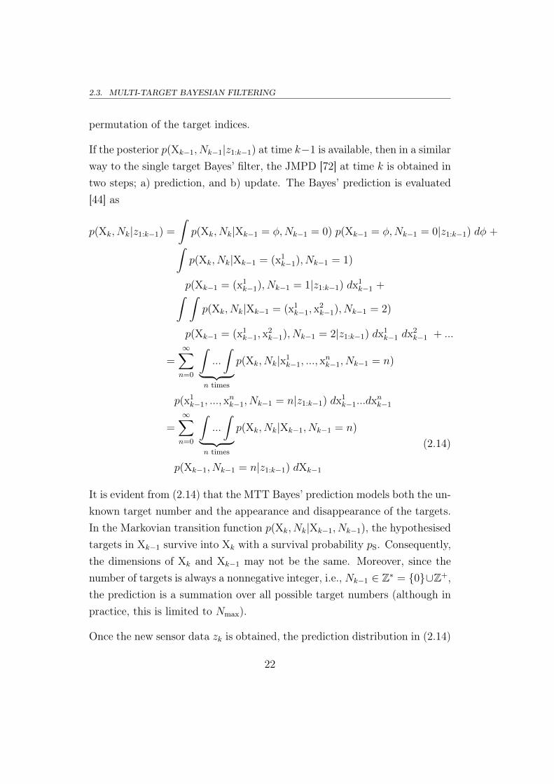
If the posterior p(Xk−1, Nk−1|z1:k−1) at time k−1 is available, then in a similarway to the single target Bayes’ filter, the JMPD [72] at time k is obtained intwo steps; a) prediction, and b) update. The Bayes’ prediction is evaluated[44] as
p(Xk, Nk|z1:k−1) =
∫p(Xk, Nk|Xk−1 = φ,Nk−1 = 0) p(Xk−1 = φ,Nk−1 = 0|z1:k−1) dφ +∫p(Xk, Nk|Xk−1 = (x1
k−1), Nk−1 = 1)
p(Xk−1 = (x1k−1), Nk−1 = 1|z1:k−1) dx1
k−1 +∫ ∫p(Xk, Nk|Xk−1 = (x1
k−1, x2k−1), Nk−1 = 2)
p(Xk−1 = (x1k−1, x
2k−1), Nk−1 = 2|z1:k−1) dx1
k−1 dx2k−1 + ...
=∞∑n=0
∫...
∫︸ ︷︷ ︸n times
p(Xk, Nk|x1k−1, ..., x
nk−1, Nk−1 = n)
p(x1k−1, ..., x
nk−1, Nk−1 = n|z1:k−1) dx1
k−1...dxnk−1
=∞∑n=0
∫...
∫︸ ︷︷ ︸n times
p(Xk, Nk|Xk−1, Nk−1 = n)
p(Xk−1, Nk−1 = n|z1:k−1) dXk−1
(2.14)
It is evident from (2.14) that the MTT Bayes’ prediction models both the un-known target number and the appearance and disappearance of the targets.In the Markovian transition function p(Xk, Nk|Xk−1, Nk−1), the hypothesisedtargets in Xk−1 survive into Xk with a survival probability pS. Consequently,the dimensions of Xk and Xk−1 may not be the same. Moreover, since thenumber of targets is always a nonnegative integer, i.e., Nk−1 ∈ Z∗ = {0}∪Z+,the prediction is a summation over all possible target numbers (although inpractice, this is limited to Nmax).
Once the new sensor data zk is obtained, the prediction distribution in (2.14)
22
CHAPTER 2. BAYESIAN FILTERING
is updated using Bayes’ rule according to
p(Xk, Nk|z1:k) =p(zk|Xk, Nk)p(Xk, Nk|z1:k−1)
p(zk|z1:k−1)(2.15)
where p(zk|Xk) is the likelihood function and p(zk|z1:k−1) is a normalisingconstant. The recurrence of (2.14) and (2.15) is the property that forms thebasis for the Bayes’ MTT filter.
To estimate the joint target state and the target number from p(Xk, Nk|z1:k),the marginal multi-target (MaM) estimator may be used3: here, the marginaldistribution of Nk is formed according to
p(Nk|zk) ,∫p(Xk, Nk|z1:k)dXk (2.16)
Then the expected number of targets is the MAP estimate
Nk , arg supNk p(Nk|zk) (2.17)
and the MaM estimate of the joint target state is obtained using
XMaMk , arg sup
x1k,...,x
Nkk
p(x1k, ..., x
Nkk |z1:k) (2.18)
Under the assumptions that; a) the number of targets at each time step isknown, and b) targets neither appear or disappear, the Bayes’ MTT predic-tion and update formalism [44] is simply a generalised form of that of thesingle target Bayes’ filter and can be written as
p(Xk|z1:k) =p(zk|Xk)
p(zk|z1:k−1)
∫p(Xk|Xk−1) p(Xk−1|z1:k−1) dXk−1 (2.19)
2.3.3 Implications of the sensor model for the likelihood
Here, the implications of the choice of the sensor feed zk on evaluating thelikelihood function p(zk|Xk) in (2.15) are discussed.
3Other Bayes’ MTT estimators can be found in Ch. 14 of [32].
23
2.3. MULTI-TARGET BAYESIAN FILTERING
Data association approach
In traditional surveillance systems, the direct information received at the sig-nal processing unit is usually; (i) a image (e.g., SONAR image), or (ii) asignal (e.g., acoustic signal). In many tracking applications, this informa-tion is further processed to generate M noisy point target detections whichthen are the observation feed to the filter. This input feed contains targetdetections, false alarms4 or clutter5 and is expressed as
Zk = {z1k, ..., z
Mk } (2.20)
where the mth measurement zmk ∈ Z (recall from section 2.1 that Z is thesingle target observation space). Here, it is assumed that multiple targetscannot generate one point target observation. Hence, while evaluating thelikelihood in (2.15), it is important to know which measurement in Zk re-lates to which target hypothesis in Xk — the data association. The use ofthe observation model in (2.20) casts the MTT problem into two domains:a) filtering, and b) data association. Data association [73] aids in identifyingclose targets and avoiding confusing them, for example, aircraft flying close[1].
One method of achieving data association is by multiple hypothesis track-ing (MHT) [74]. The MHT filter operates by first creating hypotheses aboutall the possible associations between the sensor detections and the targetstates, and then choosing one hypothesis based on its weight, interpretedas the probability that it is the correct one. A few measures that computethe probability of a hypothesis being correct are the Mahanalobis distanceor global association distance [32]. This method, however, is computation-ally expensive as it propagates all the possible hypotheses every time step.Another approach to data association is joint probabilistic data association
4False alarms are sensor detections that did not originate from the targets, but arecaused by noise.
5Clutter are sensor detections from objects which are not of interest, e.g., for a satelliteobserving sensor, stars are the clutter.
24

CHAPTER 2. BAYESIAN FILTERING
(JPDA) [43] in which all the potential target-measurement associations aretreated as a single statistical unit, i.e., all measurements are assumed to beassociated to every target to some extent [27]. The JPDA filter [5, 10, 11]computes the degree to which each measurement contributed to each targetand then creates composite tracks that represent the correct one.
Association free approach
Much work on MTT and information fusion relates to observations which arepoint target detections described in (2.20). However, converting sensor datainto point target measurements using pre-processing tools like thresholdingintroduces substantial information loss, especially at low signal-to-noise ratio(SNR). In contrast, feeding the raw information (image or signals) from thesensors directly to the filter allows merged observations — multiple targetsgenerating the one observation datum6 [44]. This avoids data association andhence overcomes the combinatorial problem of target-measurement associa-tion.
2.3.4 Curse of dimensionality
Since the JMPD p(Xk|z1:k) provides complete information about the multi-target scenario at time k, the filtering is considered optimal. However thefilter suffers from high computational complexity:
Example: Consider that targets lie in the discrete 1D space X = {1, 2, ..., 10}.In a single target scenario, the state space contains 10 values and the dimen-sionality of xk is 1, for example, xk = 3. However, in a two target scenario,the joint state space X∗ = X×X will now contain 100 values and the dimen-sionality of the joint state Xk is 2, for example, Xk = (3, 7).
6Examples of merged observations: a) in a image, the intensity of a single pixel couldbe influenced by multiple targets, and b) in a phased sensor array, signals from multiplesignals are added at the sensors.
25

2.4. THE KALMAN FILTER
If tracking involved computing the probability of each possible combinationof states, then it is evident that the computational effort devoted to evalu-ate the joint pdf worsens exponentially. This complexity problem, conven-tionally termed “curse of dimensionality 7,” [45] makes the filtering processintractable.
2.4 The Kalman filter
The computational intractability of the Bayes’ filter is overcome using ap-proximate solutions. A popular Bayes’ filter which provides a closed-formsolution to target state estimation is the Kalman filter [20]. In this section,the Kalman filter that conceptualises Bayes’ recursion in a discrete time lin-ear filtering perspective is presented. The filter’s mathematical treatment isoutlined in section 2.4.1 which is followed by a brief survey of its historicaldevelopment in section 2.4.2.
Kalman filtering is regarded as a least square estimation process withprovision to model the dynamic stochastic target state8. Consequently itssolution is optimal. The filter assumes that the posterior pdf is Gaussiandistributed at every time step [5] and hence can be parameterised by a meanand a covariance. The Gaussianity assumption in the Kalman filter will beconsistent with time [78] under the following conditions:
1. The process and observation noise sequences qk−1 in (2.2) and rk in(2.3) respectively are drawn from Gaussian distributions with knownparameters,
2. (2.2) and (2.3) are known linear functions.
7The term was coined by R. E. Bellman in 1957 when considering dynamic optimisationproblems [75, 76].
8In other words, Kalman filter is a time variant Wiener filter [77].
26

CHAPTER 2. BAYESIAN FILTERING
Hence, the process and observation models can be re-written as
xk = Fkxk−1 + qk−1 (2.21)
zk = Hkxk + rk (2.22)
where Fk and Hk are linear functions. The noise sequences qk−1 and rk
are random samples drawn from the distributions N (0, Qk−1) and N (0, Rk)
respectively. If these conditions are not met, the Kalman filter can still beused, but is regarded in that case as a second order moment approximation tothe single target Bayes’ filter. The single target posterior p(xk|z1:k), under theassumption that it is essentially Gaussian and not skewed, can be compressedinto its approximate sufficient statistics — the first and second moments as
p(xk|z1:k) = N (xk, Pk) (2.23)
with mean xk and covariance Pk, the closed-form of which is presented in thefollowing section.
2.4.1 The Kalman filter recursion
The derivation of the Kalman filter [20, 32, 79, 80] is not central to this the-sis and is not provided here. The Kalman filter describes the posteriorp(xk−1|z1:k−1) at time k − 1 as a Gaussian. Hence the filter is parameterisedby the mean xk−1 and its error covariance Pk−1. At the next time index k,the filter operates in two stages; (i) prediction, in which the a priori stateestimate x
′
k and its error covariance P ′k are computed, and (ii) update, inwhich the a posteriori state estimate xk and its error covariance Pk are com-puted.
The filter recursion from time k − 1 to k can be expressed as
p(xk−1|z1:k−1) = N (xk−1, Pk−1) (2.24)
p(xk|z1:k−1) = N (x′
k, P′
k) (2.25)
p(xk|z1:k) = N (xk, Pk) (2.26)
27
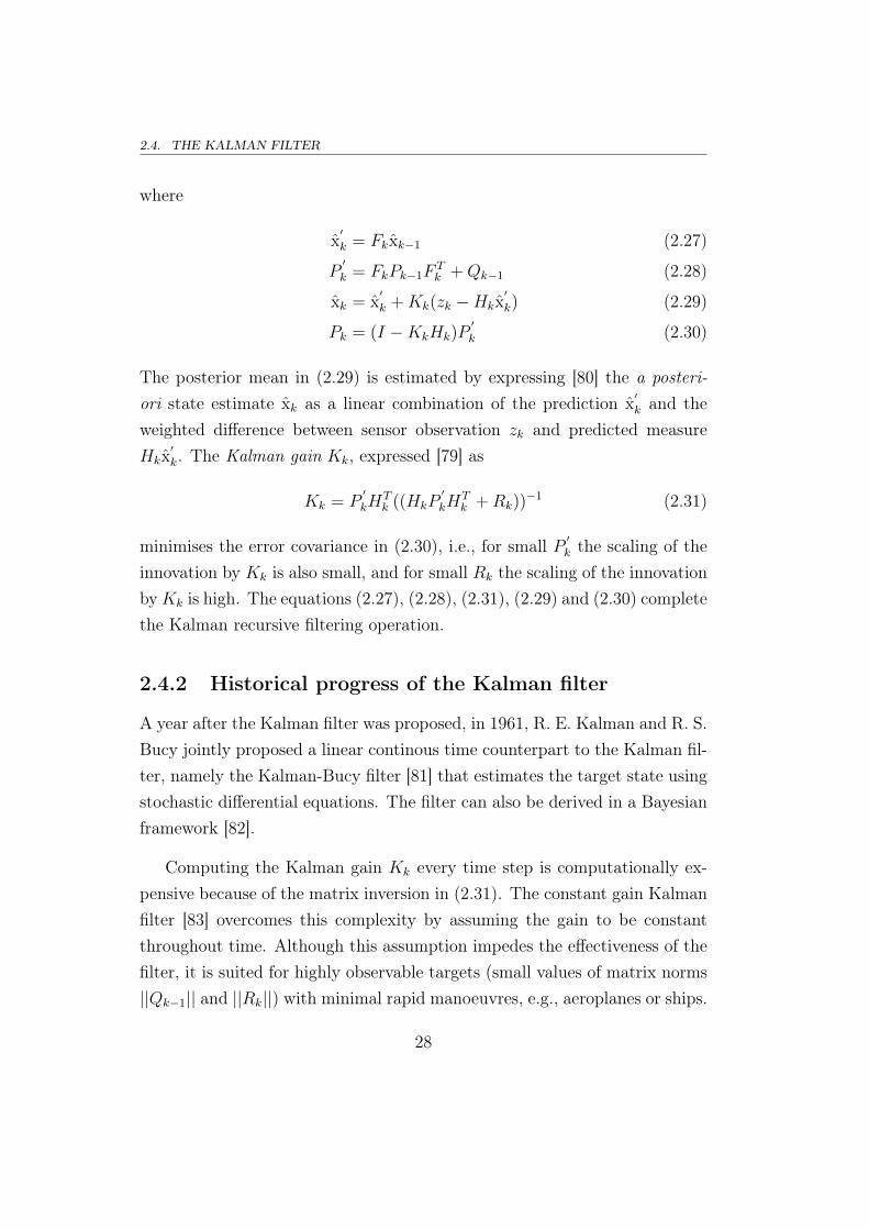
2.4. THE KALMAN FILTER
where
x′
k = Fkxk−1 (2.27)
P′
k = FkPk−1FTk +Qk−1 (2.28)
xk = x′
k +Kk(zk −Hkx′
k) (2.29)
Pk = (I −KkHk)P′
k (2.30)
The posterior mean in (2.29) is estimated by expressing [80] the a posteri-ori state estimate xk as a linear combination of the prediction x
′
k and theweighted difference between sensor observation zk and predicted measureHkx
′
k. The Kalman gain Kk, expressed [79] as
Kk = P′
kHTk ((HkP
′
kHTk +Rk))
−1 (2.31)
minimises the error covariance in (2.30), i.e., for small P ′k the scaling of theinnovation by Kk is also small, and for small Rk the scaling of the innovationbyKk is high. The equations (2.27), (2.28), (2.31), (2.29) and (2.30) completethe Kalman recursive filtering operation.
2.4.2 Historical progress of the Kalman filter
A year after the Kalman filter was proposed, in 1961, R. E. Kalman and R. S.Bucy jointly proposed a linear continous time counterpart to the Kalman fil-ter, namely the Kalman-Bucy filter [81] that estimates the target state usingstochastic differential equations. The filter can also be derived in a Bayesianframework [82].
Computing the Kalman gain Kk every time step is computationally ex-pensive because of the matrix inversion in (2.31). The constant gain Kalmanfilter [83] overcomes this complexity by assuming the gain to be constantthroughout time. Although this assumption impedes the effectiveness of thefilter, it is suited for highly observable targets (small values of matrix norms||Qk−1|| and ||Rk||) with minimal rapid manoeuvres, e.g., aeroplanes or ships.
28

CHAPTER 2. BAYESIAN FILTERING
Alpha-Beta filters [84] are one example of the constant gain Kalman filter.Appending additional information like sensor bias, blurring of targets due tobad weather, etc., to the target state vector improves knowledge about theuncertainty of the estimate. The Schmidt-Kalman filter [85] accomplishesthis information improvement without the need to increase the dimensional-ity of the state vector and thereby reduces complexity.
Given that the Kalman filter is limited to linear Gaussian target systems,noteworthy effort has been made to derive optimal non-linear filters, e.g.,[86–89]. Additionally, several sub-optimal versions have been proposed tothe Kalman filter to adapt it for non-linear systems. The extended Kalmanfilter (EKF) [90] extends the Kalman filter to non-linear systems by linearis-ing about an estimate of the current mean and covariance. Here the statedistribution is approximated by a Gaussian random variable and then propa-gated through the first order Taylor series expansion of the non-linear system[91] in order to calculate the mean and covariance. Higher order EKFs areobtained by retaining more terms of the Taylor series expansion. The un-scented Kalman filter (UKF) [92, 93] approximates the Gaussian target staterandom process by a set of carefully chosen sample points that capture thetrue mean and covariance [94]. These points, when propagated in a non-linear system, capture the true mean and covariance accurately up to secondorder [95] (only for scalar states [96]). A summary of numerous other variantsto Kalman filtering can be found in [97]. The EKF, UKF and other variantsalways approximate the posterior to be Gaussian, and introduce significantbias if the actual distribution is non-Gaussian; they cannot model the higherorder moments of non-Gaussian posterior distributions.
The Kalman filter for MTT will generate a target state estimate (mean)and covariance estimate for each of the targets present in the scene. How-ever, it is important to relate the sensor observations to each of the targets— the data association. The problem of data association is treated in threeways: firstly, the single hypothesis correlation (SHC) technique builds a track
29

2.5. THE SEQUENTIAL MONTE CARLO
table containing the state estimate and the error covariance for each target,and updates them based on the minimum association distance between eachtarget and each sensor using the Mahanalobis distance, given by
d(xpk|zk) , (zk −Hkxpk)T (HkP
pkH
Tk +Rk)
−1 (zk −Hkxpk) (2.32)
where xpk and P pk are the state and the error covariance of the pth target
respectively. In other words, the SHC can be visualised as a bank of par-allel Kalman filters, one for each target, with filters being removed if theircovariance estimate crosses a certain threshold. The SHC filter is forcedto declare that a single measurement target association is correct, which isnot an optimal representation when uncertainty in the association is sig-nificant. A second approach to data association is the multiple hypothesistracking (MHT) [74] filter; however, as mentioned in section 2.3, this methodinvolves high computational cost. Thirdly, the composite hypothesis correla-tion (CHC) [32] filter uses the concept of the JPDA and computes the bestpossible target-measurement association by using a joint formulation of allthe association hypotheses.
The Kalman filter has been widely used in several array processing ap-plications, a few examples of which include: positioning of ships [98], under-water submarine navigation [99], underwater SONAR tracking [100], rainfallestimation [101], detecting signals from buried objects [102], tracking seabedparameters [103], recording seismic activity [104], localisation using micro-phone arrays [105], spacecraft tracking [106], guiding satellites into theirorbits [107] and estimating heart-beat [4].
2.5 The sequential Monte Carlo
The high dimensional integration in the Bayes’ recursive solution makes theprocess computationally intractable. However, the exact closed-form solutionto Bayes’ filtering for linear Gaussian systems is possible using the Kalmanfilter described in section 2.4. In the current and subsequent sections, Bayes’
30
CHAPTER 2. BAYESIAN FILTERING
approximations for more realistic non-linear and non-Gaussian systems arepresented. These approaches provide only approximate solutions and henceare sub-optimal.
A prominent Bayesian approximation is the sequential Monte Carlo (SMC)approach. Monte Carlo9 is a stochastic sampling approach aimed at tacklingdifficult numerical integration problems. Since their first use in 1949 byMetropolis and Ulam [22] in the Los Alamos laboratory, Monte Carlo meth-ods have been explored to address many intractable problems in physics andstatistics [108]. The SMC, which is a combination of Monte Carlo samplingand Bayesian statistics, is a powerful tool for online estimation of Markoviantarget systems. The formal introduction of Monte Carlo to Bayesian targettracking was made in 1993 by Gordon et al. and the resulting method iscalled the particle filter (PF) [21]. The PF belongs to the class of SMC [109]methods and approximates the probability distributions using independentpoint mass representations — also called samples or particles. These particlesare sampled directly from the state space and weighted through the principleof importance sampling. The recursive propagation of this particle systemresults in an accurate Bayesian approximation [110, 111]. The primary focusof this thesis is the development of PF schemes to overcome various limita-tions in Bayesian MTT for array processing applications. Hence the filteris discussed in detail. Monte Carlo importance sampling is first introducedin sections 2.5.1 and 2.5.2. This is followed by the PF and its operationalissues in sections 2.5.3, 2.5.4 and 2.5.6. A variant of the PF which will befurther referred to in this thesis is then outlined in section 2.5.7. Finally, thehistorical developments of the PF are discussed in section 2.5.8.
2.5.1 Monte Carlo sampling
Here, Monte Carlo sampling is introduced using a simple derivation. Considera statistical problem of estimating the expected value of a function g(x). This
9Named after Monte Carlo Casino in Monaco.
31

2.5. THE SEQUENTIAL MONTE CARLO
can also be considered as estimating a Lebesgue-Stieltjes integral
E[g(x)] =
∫x
g(x) dp(x) (2.33)
where the integration of g → R is defined with respect to a Lebesgue mea-sure [112]. If g(x) is intractable, then the computation of E[g(x)] is dif-ficult. Monte Carlo sampling could be employed to treat such situations.The method approximates E[g(x)] using a set of independent and identi-cally distributed (i.i.d) samples (also called particles) {x1, ..., xI}, where fori = 1, ..., I
xi ∼ p(.) (2.34)
Then the Monte Carlo estimate of g(x) is
g =1
I
I∑i=1
g(xi) (2.35)
The expected value of the Monte Carlo estimate is given by
E[g] = E[1
I
I∑i=1
g(xi)]
=1
IE[ I∑i=1
g(xi)]
=1
I
I∑i=1
E[g(xi)]
= E[g(x)] (2.36)
32

CHAPTER 2. BAYESIAN FILTERING
and the variance of the Monte Carlo estimate is given by
var[g] = var[1
I
I∑i=1
g(xi)]
=1
I2var[ I∑i=1
g(xi)]
=1
I2
I∑i=1
var[g(xi)]
=I
I2var[g(x)]
=var[g(x)]
I(2.37)
By the strong law of large numbers [113, 114], the Monte Carlo estimate gconverges to the true value of E[g(x)] in (2.33) as I → ∞. Monte Carlosampling, by itself, cannot be employed in Bayesian filtering because thefunction p(x) from which particles are drawn is unknown. This problemis addressed by importance sampling, which is described in the followingsection.
2.5.2 Importance sampling
Importance sampling aims to represent p(x) by drawing a set of weightedparticles {xi, wi}Ii=1 (I is the total number of particles) from regions of “im-portance” in the distribution. This is achieved by drawing from a proposal orimportance distribution q(x) that is similar to p(x). Discussion on the choiceof q(x) is deferred until section 2.5.6. Consider the integral∫
g(x)p(x)dx =
∫g(x)
p(x)
q(x)q(x)dx (2.38)
The Monte Carlo representation of p(x) is expressed as
p(x) ≈I∑i=1
wi δ(x− xi) (2.39)
33

2.5. THE SEQUENTIAL MONTE CARLO
where the weights (also called importance weights) are
wi =p(xi)
q(xi)(2.40)
If the normalising factor of p(x) is not known, the importance weights canonly be calculated up to a normalising constant. The weights are normalisedto ensure that
∑Ii=1w
i = 1. Then the Monte Carlo estimate to the filteredstate moment E[g(x)] is
g =1
I
(∑Ii=1 w
ig(xi)∑Ii=1 w
i
)(2.41)
and the variance of the importance sampling estimate is
var(g) =1
Ivar[g(x) w]
=1
Ivar[g(x)
p(x)
q(x)
]=
1
I
∫ [g(x)p(x)
q(x)− E[g]
]2
q(x)dx
=1
I
∫ [(g(x)p(x))2
q(x)− 2g(x)p(x)E[g]
]dx +
(E[g])2
I
=1
I
(∫ [(g(x)p(x))2
q(x)
]dx− (E[g])2
)(2.42)
It is obvious from (2.42) that the variance of the Monte Carlo estimate isminimised when q(x) matches p(x). Moreover, according to the weak law oflarge numbers [115], it is found that
g → E[g(x) w]
E[w](2.43)
Returning to Bayes’ filtering, the posterior p(xk|z1:k) is the true pdf, the non-linearity and/or non-Gaussianity of which makes it difficult to draw particlesfrom. However, p(xk|z1:k) can be represented using a weighted particle set{xik, wik}Ii=1, where I is the total number of particles, drawn from a known
34

CHAPTER 2. BAYESIAN FILTERING
proposal distribution q(xk|z1:k). The importance weights of these particles,as in (2.40) is
wik =p(xik|z1:k)
q(xik|z1:k)(2.44)
Propogating these weighted particles sequentially in a Bayes’ framework isperformed by sequential importance sampling (SIS), which is described inthe following section.
2.5.3 Sequential importance sampling
Consider that the weighted particles {xik−1, wik−1}Ii=1 that represent p(xk−1|z1:k−1)
at time k−1 are available. The aim of SIS is to obtain {xik, wik}Ii=1 that repre-sent the posterior p(xk|z1:k) at the next time step k. This is accomplished bydrawing particles from a known importance distribution q(xk|z1:k). The pro-cess is done in two steps; a) prediction, and b) update. The prediction steppropagates the particles {xik−1}Ii=1 to time step k as follows: the importancedistribution can be factorised as
q(x1:k|z1:k) = q(xk|x1:k−1, z1:k)q(x1:k−1|z1:k−1) (2.45)
This implies that particles xik−1 ∼ q(xk−1|z1:k−1) are propagated to time k byaugmenting their states by another set of particles drawn from
xik ∼ q(xk|xk−1, zk) ; i = 1, ..., I (2.46)
35

2.5. THE SEQUENTIAL MONTE CARLO
The update step evaluates the weights of {xik}Ii=1 using the new sensor evi-dence zk. This is done as follows: the posterior pdf
p(x1:k|z1:k) =p(z1:k|x1:k)p(x1:k)
p(z1:k)
=p(zk, z1:k−1|x1:k)p(x1:k)
p(zk, z1:k−1)
=p(zk|z1:k−1, x1:k)p(z1:k−1|x1:k)p(x1:k)
p(zk|z1:k−1)p(z1:k−1)
=p(zk|z1:k−1, x1:k)p(x1:k|z1:k−1)p(z1:k−1)p(x1:k)
p(zk|z1:k−1)p(z1:k−1)p(x1:k)
=p(zk|xk)p(x1:k|z1:k−1)
p(zk|z1:k−1)
=p(zk|xk)p(xk, x1:k−1|z1:k−1)
p(zk|z1:k−1)
=p(zk|xk)p(xk|x1:k−1, z1:k−1)p(x1:k−1|z1:k−1)
p(zk|z1:k−1)
=p(zk|xk)p(xk|x1:k−1)p(x1:k−1|z1:k−1)
p(zk|z1:k−1)
∝ p(zk|xk)p(xk|x1:k−1)p(x1:k−1|z1:k−1) (2.47)
By substituting (2.45) and (2.47) in (2.44), the unnormalised particle weightbecomes
wik ∝p(zk|xik)p(xik|xik−1)p(xik−1|z1:k−1)
q(xik|xik−1, zk)q(xik−1|z1:k−1)
= wik−1
p(zk|xik)p(xik|xik−1)
q(xik|xik−1, zk); i = 1, ..., I (2.48)
The weights are normalised wik =wik∑Ij=1 wjk
and p(xk|z1:k) is represented by
p(xk|z1:k) ≈I∑i=1
wik δ(xk − xik) (2.49)
36
CHAPTER 2. BAYESIAN FILTERING
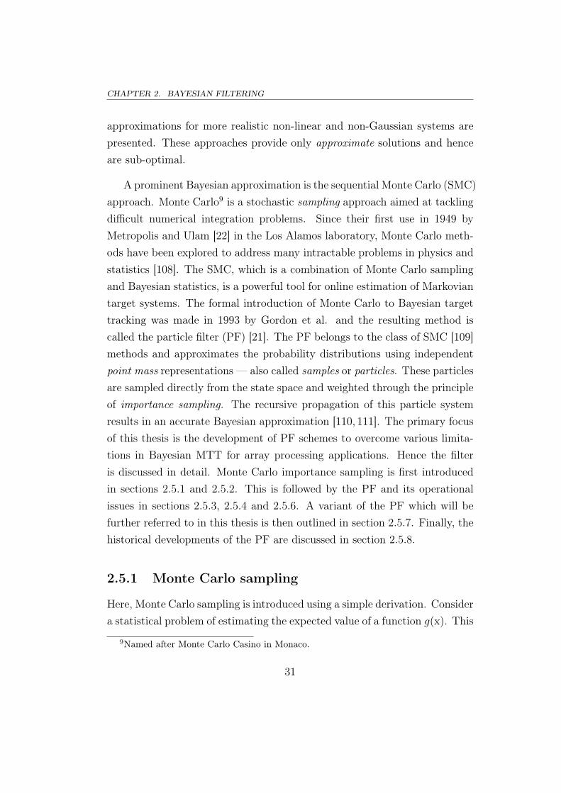
Degeneracy
As the SIS algorithm progresses, the particles near the actual target gainmore weight, and those that are far away have negligible weights. This impliesthat high computational effort is required to update these negligible weightparticles that do not contribute to the true posterior [54]. This problem iscalled degeneracy. That is, if the genealogy of a particle is observed by tracingits parent all the way to the initial time step, it can then be seen that asparticles propagate in time, it will become more likely that a single particlewill be the parent of all its descendents and this parent need not necessarilyhave high importance. This implies that one particle grabs all the weightand this particle may not necessarily contribute to the true posterior. Thisis illustrated using a simple example in Fig. 2.1.
One measure of efficiency in this context is the effective sample size [52],defined as
Ieff =1∑I
i=1(wik)2
(2.50)
such that Ieff � I and low Ieff exhibits high degeneracy. The solution todegeneracy is to resample the particles (in accordance to their weights) withreplacement whenever Ieff falls below a certain threshold [109]. This resam-pling is presented in the following section.
2.5.4 Sequential importance resampling: The PF
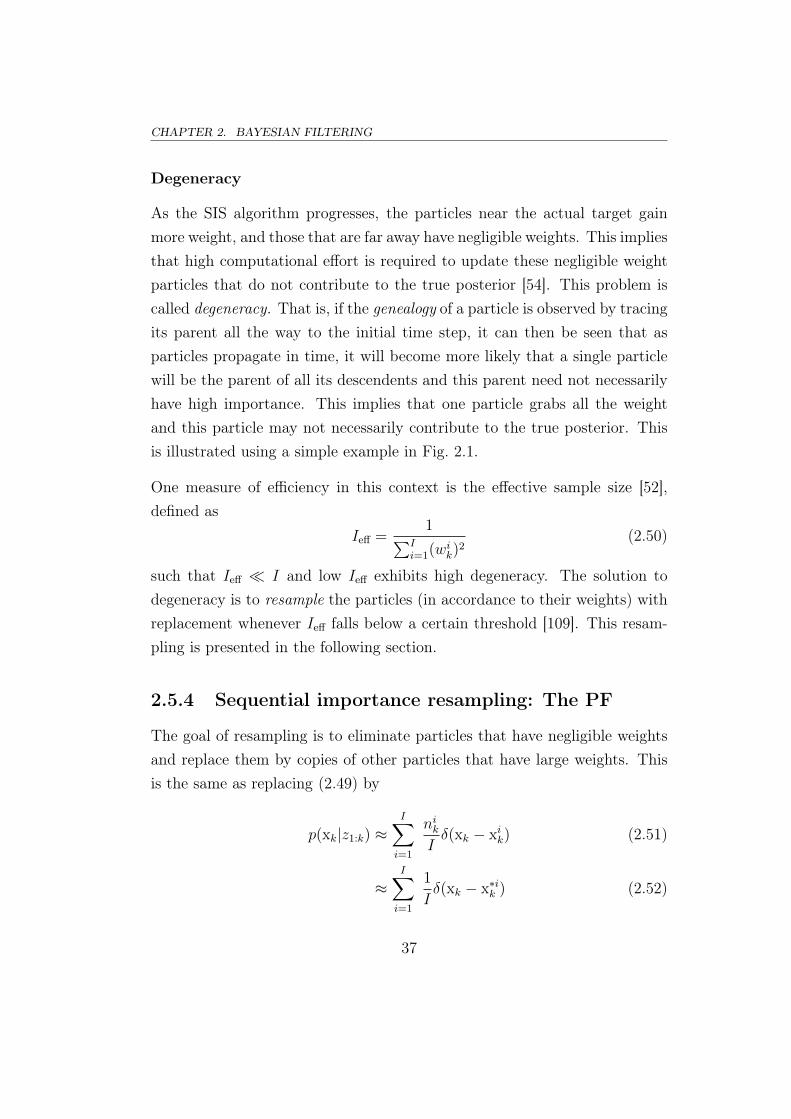
The goal of resampling is to eliminate particles that have negligible weightsand replace them by copies of other particles that have large weights. Thisis the same as replacing (2.49) by
p(xk|z1:k) ≈I∑i=1
nikIδ(xk − xik) (2.51)
≈I∑i=1
1
Iδ(xk − x∗ik ) (2.52)
37
2.5. THE SEQUENTIAL MONTE CARLO
2 4 6 8 10 12 14
−40
−20
0
20
40
60
Po
sitio
n [
m]
Time [s]
Ground truth
Particle genealogy
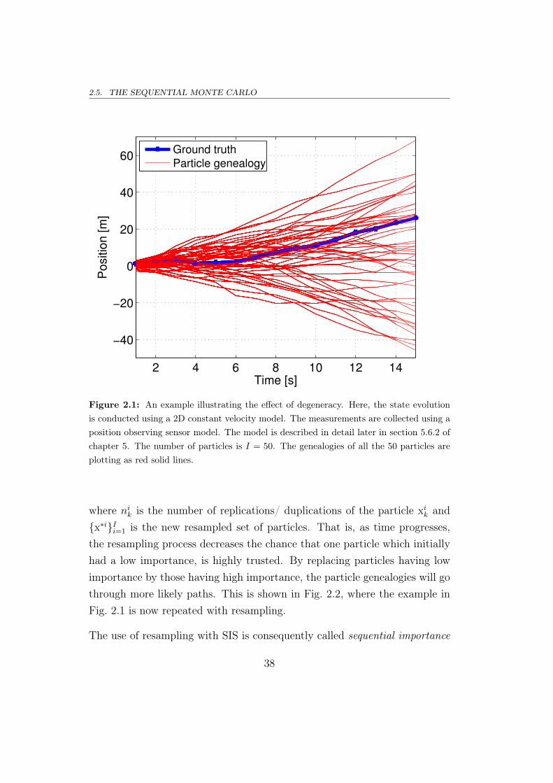
Figure 2.1: An example illustrating the effect of degeneracy. Here, the state evolutionis conducted using a 2D constant velocity model. The measurements are collected using aposition observing sensor model. The model is described in detail later in section 5.6.2 ofchapter 5. The number of particles is I = 50. The genealogies of all the 50 particles areplotting as red solid lines.
where nik is the number of replications/ duplications of the particle xik and{x∗i}Ii=1 is the new resampled set of particles. That is, as time progresses,the resampling process decreases the chance that one particle which initiallyhad a low importance, is highly trusted. By replacing particles having lowimportance by those having high importance, the particle genealogies will gothrough more likely paths. This is shown in Fig. 2.2, where the example inFig. 2.1 is now repeated with resampling.
The use of resampling with SIS is consequently called sequential importance
38

CHAPTER 2. BAYESIAN FILTERING
resampling (SISR) or PF10. Although resampling reduces the degeneracyproblem by discarding those particles that do not contribute to the poste-rior, it could lead to particle impoverishment — a problem in which very fewparticles get replicated many times thereby reducing the richness (or diver-sity) of the particles in effectively representing the posterior: some methodsthat overcome this problem are discussed briefly in section 2.5.8. Being anapproximation technique, the PF converges almost definitely to the true pos-terior as I →∞. Convergence results for the PF can be found in [116, 117].
2 4 6 8 10 12 140
5
10
15
20
25
Po
sitio
n [
m]
Time [s]
Ground truth
Particle genealogy
Figure 2.2: An example illustrating how resampling overcomes the effect of degeneracy.The ground truth, process and measurement model and sample size I are the same as usedin Fig. 2.1.
10Various other names for the PF are bootstrap filtering, condensation algorithm andsurvival of the fittest.
39
2.5. THE SEQUENTIAL MONTE CARLO
Resampling techniques are majorly divided into two classes; a) stochastic,and b) deterministic. Detailed studies on resampling algorithms can be foundin [118–121]. A few popular resampling techniques, that will be referred toin chapter 5 are presented here.
Multinomial selection
The aim of stochastic resampling is the multinomial selection of nik in (2.51)which is equivalent to selecting x∗j for j = 1, ..., I particles, such that P (x∗j =
xi) = wi, i.e., the particles are resampled in accordance to their weights. Thismultinomial selection can be done as follows
• Draw a random sample uik ∼ U(0, 1],
• Assign index j ← i such that∑i−1
s=1wsk < uik ≤
∑is=1w
sk.
In the resampling literature, there are four variations of this multinomialselection. These variants are briefly discussed here.
1. Multinomial resampling: This method is simply the conventionalmultinomial selection scheme and also termed random resampling. Here,draw I random samples uk, each drawn according to uik ∼ U(0, 1]. Thenallocate nik copies of xik to the new distribution according to
nik = the number of uk ∈
(i−1∑s=1
wsk,
i∑s=1
wsk
](2.53)
This process is equivalent to the two-step multinomial selection process de-scribed above. (2.53) also ensures that
∑Ii=1 n
ik = I. Finally, the weights of
the new set of particles are set to 1/I.
2. Stratified resampling: The process of creating the random samplesuk by sampling I times from the space (0, I] leads to a high Monte Carlo(MC) variance. Stratified resampling is motivated by the idea that creatinguk by sampling I times, once from each of the I independent ordered subsets
40

CHAPTER 2. BAYESIAN FILTERING
of equal size(iI, i+1
I
]for i = 0, ..., I − 1, will reduce the MC variance. The
space (0, I] which is now divided into I disjoint subsets is referred to as strata.The selection of the random samples is conducted independently within eachstratum, i.e., uk is obtained by sampling I times, once from from each ofthe I ordered subsets. Hence stratified resampling is similar to multinomialresampling in (2.53), except that now, the random samples are
uik =(i− 1) + uik
Iwith uik ∼ U(0, 1], i = 0, ..., I − 1 (2.54)
The weights of the new set of particles are set to 1/I.
3. Systematic resampling: This method aims to further reduce the MCvariance. The procedure is almost similar to that of stratified resampling:the stratification process is unchanged, but the random samples drawn fromthe strata are no longer independent, i.e., all samples have the same positionwithin each stratum. Hence systematic resampling is similar to multinomialresampling in (2.53), except that now, the random samples are
uik =(i− 1) + uk
I, i = 0, ..., I − 1 (2.55)
with uk ∼ U(0, 1]. The weights of the new set of particles are set to 1/I.
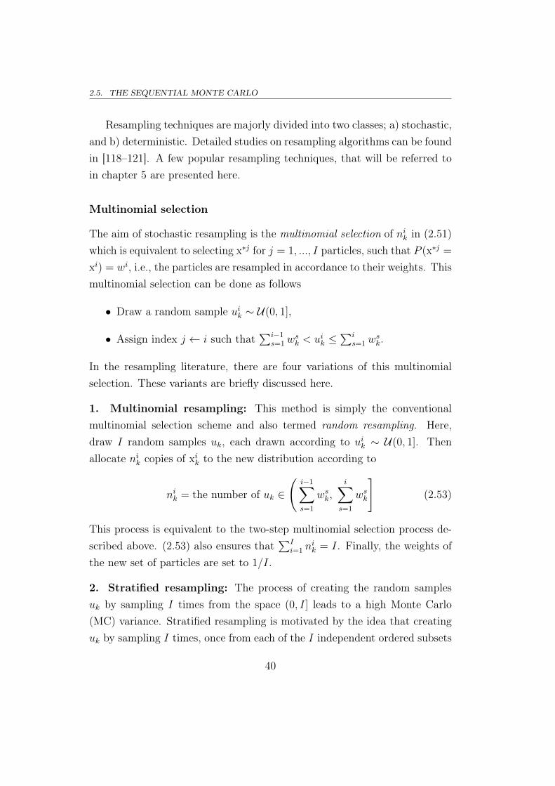
Example illustration: The process of selecting the random samples uk ineach of the above mentioned methods is illustrated in Fig. 2.3 using a simpleexample. Here, the grey solid line is the cumulative sum of the weights of I =
5 particles. The weight vector is chosen to be wk = [0.1, 0.2, 0.5, 0.15, 0.05].The space from which random samples are drawn is spanned by the red dou-ble arrow(s). The random sample values are pointed using the I blue arrows.In multinomial resampling, each random sample is drawn from the space(0, I] (shown using a single red double arrow) according to uik ∼ U(0, I].In stratified resampling, the space (0, I] is stratified into I disjoint subsets(shown using I red double arrows) and the random samples are drawn in-dependently from each strata according to (2.54). In systematic resampling,the stratification is unchanged (shown using I red double arrows) but the
41
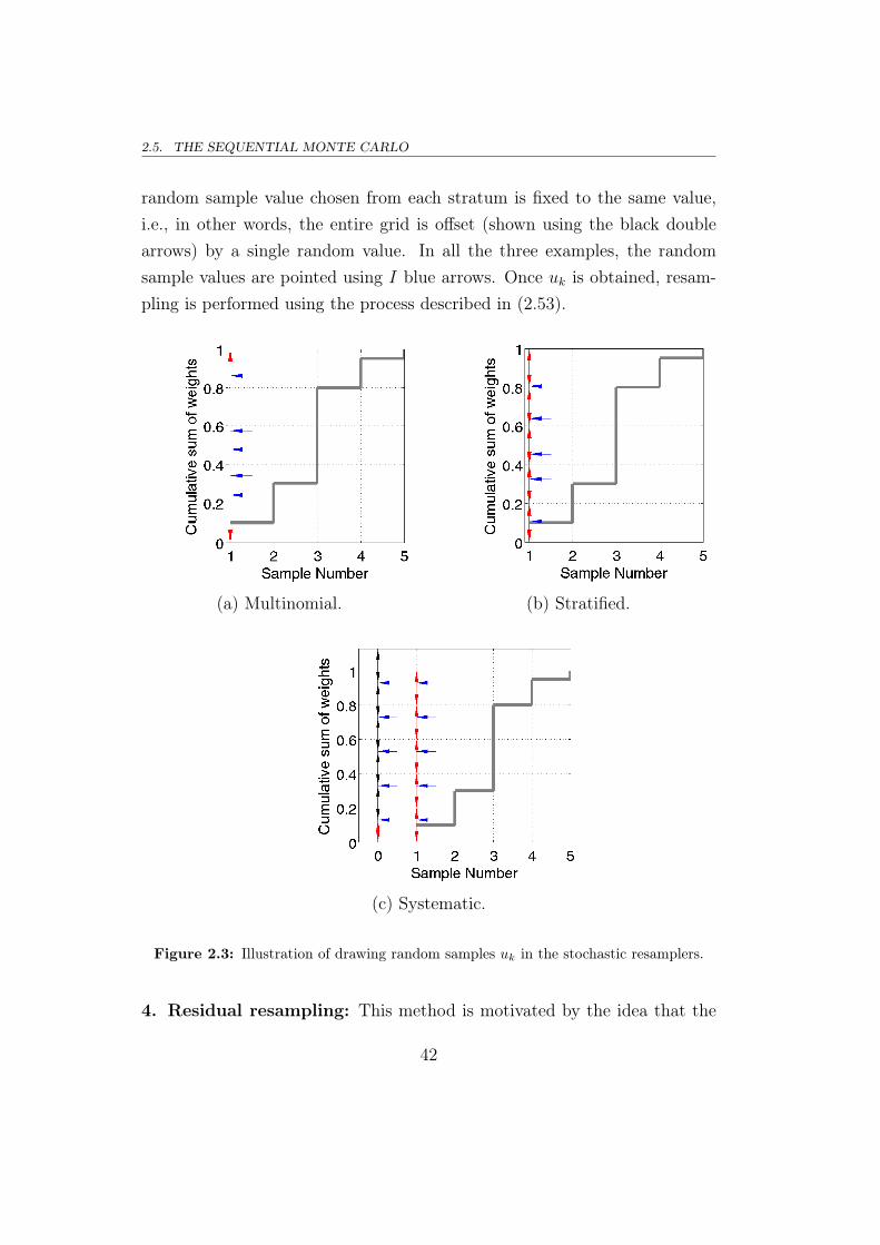
2.5. THE SEQUENTIAL MONTE CARLO
random sample value chosen from each stratum is fixed to the same value,i.e., in other words, the entire grid is offset (shown using the black doublearrows) by a single random value. In all the three examples, the randomsample values are pointed using I blue arrows. Once uk is obtained, resam-pling is performed using the process described in (2.53).
(a) Multinomial. (b) Stratified.
(c) Systematic.
Figure 2.3: Illustration of drawing random samples uk in the stochastic resamplers.
4. Residual resampling: This method is motivated by the idea that the
42

CHAPTER 2. BAYESIAN FILTERING
number of replications of many weights can be computed without stochas-ticity. Here, the number of replications nik of xik is given by bIwikc andK =
∑Ii=1bIwikc. In general K < I and the original sample size I could
be retained by stochastically resampling the K new particles to obtain theremainig I −K new particles.
Partial deterministic resampling
The second class of resampling is deterministic, which is threshold based.A hybrid between deterministic and stochastic resampling is partial deter-ministic resampling [120, 122], which was proposed to reduce PF computa-tional complexity and processing time. This combined with distributed PFapproaches would aid in PF parallelisation. The general idea is this: the par-ticles are categorised using a upper threshold Th > 1/I and a lower threshold0 < Tl < Th. Those particles with weights above Th are termed dominant,those particles with weights below Tl are termed negligible, and those par-ticles with weights between the two thresholds are termed moderate. Thedominant particles are retained, the negligible particles are eliminated andthe moderate particles are resampled using any stochastic resampler.
One variant of the partial deterministic resampling is as follows: considerNh and Nl to be the number of dominant and negligible particles respec-tively. The set of dominant and negligible particles are replaced by only thedominant particles using the following rule – the first Nl−b NlNh cNh dominantparticles are replicated r = b Nl
Nhc+ 2 times and the remaining are replicated
b NlNhc+ 1 times. Each replicated dominant particle xik is reweighted as
wik =wikr
+Wl
Nh +Nl
(2.56)
where Wl is the sum of the negligible weights. The moderate particles, onthe other hand, are retained and reweighted to the same number 1/I.
The complete PF operation using 100 particles in one-dimensional scenarioat a single time step is illustrated in Fig. 2.4.
43

2.5. THE SEQUENTIAL MONTE CARLO
2 4 6 8 100
0.005
0.01
2 4 6 8 100
0.005
0.01
2 4 6 8 100
0.05
0.1
2 4 6 8 100
0.005
0.01
Figure 2.4: The Metropolis resampling method showing the Dirac delta function of theparticles. The first figure shows I = 100 equally weighted samples {xi
k−1, wik−1}Ii=1 that
represent the posterior p(xk−1|z1:k−1). The second and third figures describe the SISstage of the PF: (i) the second figure shows the predicted set of particles (obtained usinga random walk [123] process model), and (ii) the third figure shows the weight updatedset of particles (with zk = 7.2) that represent the posterior p(xk|z1:k). It can be seen thatparticles located far away from the observation obtain low importance, and propagatingthese particles in time will lead to degeneracy. The fourth figure describes the SISR stageof the PF — particles of low importance are replaced by copies of other particles that havehigh importance. The weights are then reset to 1/I. The fourth figure shows the final setof particles {xi
k, wik}Ii=1 which will be propagated to the next time step.
2.5.5 The MTT joint PF
The single target PF can be directly generalised to MTT problems [42, 110]using the joint filter approach described in section 2.3. The conventional
44
CHAPTER 2. BAYESIAN FILTERING
MTT joint PF [44, 71, 124] is presented in this section.
Similar to the single target PF, the MTT joint PF approximates the jointposterior p(Xk, Nk|z1:k) using a set of I weighted joint particles {Xi
k, wik}Ii=1.
Each particle in the mix is a hypothesis about the states of all the targets, i.e.,a particle is now a concatenation of individual target states and will trackall the targets simultaneously. The (usually) unknown number of targets Nk
is modelled as a random variable and hence is included in the particle state.A single particle is now expressed as
(Xik, N
ik) = (xi,1k , ..., x
i,N ik
k ) (2.57)
where N ik ∈ Z∗ is the number of single target hypotheses in the joint particle
Xik. Each particle is allowed to hypothesise any number of targets, i.e., N i
k
could be different (or the same) from that of another particle. During imple-mentation, it is a common practice to limit the number of individual statesin a particle to Nmax.
If the weighted joint particle set {Xik−1, w
ik−1}Ii=1 that approximates the
posterior p(Xk−1, Nk−1|z1:k−1) at time k−1 is available, the joint PF approx-imation to the posterior at time k is obtained in two steps; a) prediction,and b) update. In the prediction, a new set of particles are sampled fromthe previous ones according to
(Xik, N
ik) ∼ q(Xk, Nk|Xk−1, Nk−1, zk) (2.58)
Target appearance and disappearance can be modelled by including a survivalprobability pS for each individual target state in the joint particle — that isto say: the nth single target state vector xi,nk−1 ∈ Xi
k−1 is either; a) retainedwith probability pS and predicted into the next state, or b) eliminated withprobability 1− pS.
In the update step, the weight of the joint particle is updated as
wik = wik−1
p(zk|Xk, Nk)p(Xk, Nk|Xk−1, Nk−1)
q(Xk, Nk|Xk−1, Nk−1, zk)(2.59)
45

2.5. THE SEQUENTIAL MONTE CARLO
Then the weights are normalised wik =wik∑Ij=1 wjk
and the posterior p(Xk, Nk|z1:k)
is approximated as
p(Xk, Nk|z1:k) ≈
∑I
i=1 wik δ(Xk − Xi
k) if dim(Xk) = dim(Xik)
0 otherwise(2.60)
To overcome degeneracy, the I joint particles are resampled with replacementbased on their weights. This resampling can be performed using any of thetechniques described in section 2.5.4. This joint MTT PF, however, suffersfrom data association and high computational complexity problems. AnotherPF approach to MTT is to use a separate filter for each target [125], but thiscould easily lead to filter hijack — a problem where more than one filtertracks one of the targets [80, 126]. A more detailed discussion on MTT PFlimitations and related work is made in chapter 3.
2.5.6 Choice of importance distribution
For the importance distribution to be optimal [52], it has to be exactly thesame as the actual probability distribution. An optimal importance distri-bution aids in drawing samples from regions of high likelihood. Hence,
q(xik|xik−1, zk)opt = p(xik|xik−1, zk) (2.61)
=p(zk|xik, xik−1)p(xik|xik−1)
p(zk|xik−1)(2.62)
Substituting (2.62) in (2.48)
wik ∝ wik−1 p(zk|xik−1) (2.63)
wherep(zk|xik−1) =
∫p(zk|xik)p(xk|xik−1)dxik (2.64)
Numerically evaluating (2.64) is non-trivial.
The analytic expression of the optimal importance distribution function
46

CHAPTER 2. BAYESIAN FILTERING
for Gaussian systems in which the motion model is non-linear and the obser-vation model is linear can be found in [52]. For non-linear Gaussian systems,Orton and Fitzgerald [127] proposed sub-optimal approximations to the op-timal importance distribution by using local linearisation techniques. Theparticles are sampled from a Gaussian approximation of the optimal im-portance distribution (2.61). If this approximation is reasonable, then thenumber of redundant particles are reduced so that fewer particles are re-quired.
It is always convenient to choose the Markov transition prior as the impor-tance distribution function. This approach however, is sub-optimal becausethe prediction is no longer leveraged on the new sensor evidence zk. Hence
q(xik|xik−1) ∝ p(xik|xik−1) (2.65)
Substituting (2.65) in (2.48) gives
wik ∝ wik−1 p(zk|xik) (2.66)
A few other methods that propose improved importance sampling of particlescan be found in [128–132].
2.5.7 Track-before-detect PF
The most common approach to target tracking is based on converting thedirect data from a sensor, e.g., infrared camera image, RADAR/SONARimage, signals from phased sensor array, etc., into point measurements ofthe targets. This conversion is usually done by thresholding. This processreduces the amount of information available to the Bayesian filter. Althoughthis information reduction is of little concern at high SNR, thresholding leadsto substantial information loss in high noise conditions. This information lossis particularly detrimental while detecting covert targets — those targetswhose signal components are well hidden under the noise components — forexample, stealth aircraft, ships sunk in deep waters, etc. For the detection
47

2.5. THE SEQUENTIAL MONTE CARLO
of these covert targets, it is important to track them for some time using theunthresholded data (also called raw sensor observations) before declaringtheir presence. The approach to simultaneously detect and initiate tracksusing raw sensor data is called track-before-detect (TBD). The TBD PF,developed in 2001 by Salmond and Birch [55], is introduced here and will bereferred to in chapter 5.
The target state xk, for instance, could be as described in (2.1). Thetarget manoeuvres according to the state evolution model in (2.2). Since thetarget could be present or absent in the observation space, its existence Ekis modelled by a two state Markov chain, such that
Ek =
1 if target is present
0 otherwise(2.67)
Consider the transition probabilities of target birth (a.k.a appearance) (pb)and death (a.k.a disappearance) (pd) respectively, to be
pb = Pr{Ek = 1|Ek−1 = 0} (2.68)
pd = Pr{Ek = 0|Ek−1 = 1} (2.69)
Then the transitional probability matrix is given by
ΠS =
1− pb pb
pd 1− pd
The sensor data zk could be raw images [55, 56, 133] for visual tracking orphased sensor array signals [134] for acoustic tracking. As described in (2.4)and (2.5) of section 2.2, the formal Bayes’ recursion consists of two steps,a) prediction, and b) update. If the posterior p(xk−1|z1:k−1) at time k − 1 isavailable, then the prediction (which exists only if Ek = 1) is expressed as
p(xk, Ek = 1|z1:k−1) =∫p(xk, Ek = 1|xk−1, Ek−1 = 1, z1:k−1)p(xk−1, Ek−1 = 1|z1:k−1)dxk−1 +∫p(xk, Ek = 1|xk−1, Ek−1 = 0, z1:k−1)p(xk−1, Ek−1 = 0|z1:k−1)dxk−1(2.70)
48

CHAPTER 2. BAYESIAN FILTERING
where
p(xk, Ek = 1|xk−1, Ek−1 = 1, z1:k−1)
= p(xk|xk−1, Ek = 1, Ek−1 = 1)p(Ek = 1|Ek−1 = 1)
= p(xk|xk−1, Ek = 1, Ek−1 = 1)(1− pd) (2.71)
and
p(xk, Ek = 1|xk−1, Ek−1 = 0, z1:k−1)
= p(xk|xk−1, Ek = 1, Ek−1 = 0)p(Ek = 1|Ek−1 = 0)
= pb pb(xk) (2.72)
Here, pb(xk) is the initial pdf of the target on its appearance. Then theupdate step is given by
p(xk, Ek = 1|z1:k) =p(zk|xk, Ek = 1)p(xk, Ek = 1|z1:k−1)
p(zk|z1:k−1)(2.73)
The likelihood function p(zk|xk, Ek = 1), for a Gaussian image model is de-scribed in Ch. 11 of [56], and for an array processing model is described in[127].
In the TBD PF recursion of (2.70) and (2.73), each particle xik is param-eterised by its existence Ei
k that is updated every time step using the statetransition matrix ΠS. The overall probability of target existence is measuredas
Ek =
∑Ii=1 E
ik
I(2.74)
and the target is declared present if Ek exceeds a certain threshold. Thetarget state estimate is obtained by taking the mean of all the particles forwhich Ei
k = 1.
2.5.8 Historical progress of the PF
Over the years, PFs have been rigorously researched and numerous improve-ments have been proposed, only a fraction of which are presented here. In an
49

2.5. THE SEQUENTIAL MONTE CARLO
attempt to emulate the process of drawing samples from an optimal impor-tance distribution, Pitt and Shepard [135] proposed the Auxiliary PF (APF)that resamples the particles {xik−1}Ii=1 using the evidence zk. The importancedistribution used in the APF is expressed as
q(xk, i|zk) ∝ p(zk|%i)p(xik|xik−1)wik−1 (2.75)
where %i ∼ p(xik|xik−1). Then
q(xk, i|zk) = q(i|zk)q(xk|i, zk)
= wik−1p(zk|%i)p(xik|xik−1) (2.76)
This process mimics to some degree particles being sampled from the opti-mal importance distribution. Several improvements and modifications to theAPF can be found in [110, 136, 137].
After the resampling step that reduces the variance of particles, it is pos-sible that some particles will be exact copies of others. If most particlesare identical, the richness of the particles in describing the posterior dete-riorates. If one or more Markov chain Monte Carlo (MCMC) [138] stepsare performed [127], whose invariant distribution is the posterior of interest,then the particles can be made disparate so that they better represent theposterior. Another method that improves the richness and diversity of theparticles is the regularised PF (RPF) [110] that resamples particles from acontinous distribution of p(xk|z1:k). The posterior approximation is
p(xk|z1:k) ∼I∑i=1
wik Kh(xk − xik) (2.77)
whereKh(x) =
1
hnxK(x
h
)(2.78)
is a positive regularisation kernal function, nx is the dimension of the statevector and h is the Kernel bandwidth. The unscented PF (UPF) [139] usesan unscented transform for importance sampling; this allows the predicted
50

CHAPTER 2. BAYESIAN FILTERING
particles to move into regions of high likelihood by leveraging them on thecurrent observation zk. A combined version of UPF and RPF, called the un-scented regularised PF (URPF) [140] uses unscented filtering for predictionand kernel density for resampling.
The main drawback of the PF is that sampling in high dimensionalspaces can be inefficient. Marginalising some of the variables is an exam-ple of the technique called Rao Blackwellisation [141]. A Rao-Blackwellised(a.k.a marginalised) PF [142] exploits linear Gaussian sub-structure presentin the model, and divides the components of the state accordingly. Supposethe components of xk are divided into two groups xlk and xnk such that thestate components in xlk follow a linear Gaussian model; then xlk could bemarginalised out in the posterior pdf as
p(x1:k|z1:k) = p(xlk, xnk |z1:k) = p(xlk|xn1:k, z1:k)p(x
n1:k|z1:k) (2.79)
The estimate of the first term in the right hand side (RHS) of (2.79) can beevaluated using a Kalman filter, and the second term can be approximatedusing a PF. The estimated pdf can now be represented by a weighted sumof Gaussians, where each particle has a Gaussian distribution attached toit [143]. This approach reduces the amount of computation required whenfiltering in a high dimensional space. The MPFs have found use in faultdiagnosis in aerospace systems [144], terrain aided navigation [145, 146], es-timating tyre radii and vehicle trajectory [6], and tracking of heart-beat andrespiratory rate [9, 147].
The multiple model PF (MMPF) [148, 149] is a wider range of hybrid PFthat allows non-linear modelling of distinctive parameters in the target statevector, e.g., a continous-value part (target dynamics) and a discrete-valuedpart (target intensity or measurement association). The TBD PF describedin section 2.5.7 belongs to the class of MMPFs.
The PF has been widely used in several real-time array processing applica-tions, examples of which include: localisation of remotely operated underwa-
51
2.6. THE PROBABILITY HYPOTHESIS DENSITY FILTER
ter vehicles using SONAR [150], bearings-only tracking using SONAR [151],TBD filtering using RADAR [152, 153], 3D indoor tracking using RADAR[154], detecting voice activity [155], audio source separation [156], detect-ing seismic activity [157], catching shovelnose guitarfish [2], tracking ballisticmissiles [158] and robot assisted heart diagnosis [159]. In spite of being com-putationally expensive [45, 46, 160], the PF is regarded as a well establishedBayes’ filter and still attracts great attention from the research community.
2.6 The probability hypothesis density filter
For MTT applications that require tracking of many targets, e.g., group tar-get tracking11, tracking only targets of interest in high target density, etc.,the theoretically optimal approach is the Bayes’ filter. However, it is knownfrom section 2.3 that the MTT Bayes’ filter is computationally challengingand hence is usually approximated. A Bayes’ approximation that overcomesthe predicament of high computational complexity in the presence of manytargets is the probability hypothesis density (PHD) filter. The PHD filterprovides a systematic approach to Bayes’ MTT using finite set statistics(FISST) on a random finite set (RFS) theoretic framework. While the ap-proximation of p(xk|z1:k) by its second order moment results in the Kalmanfilter, the approximation of the joint multi-target posterior p(Xk|z1:k) by itsfirst moment results in formation of the PHD [26]. The time-recursion of thePHD using sensor evidence is called PHD filtering.
In this section, RFS modelling is first introduced in section 2.6.1. Afterdescribing the PHD formation process in section 2.6.2, the PHD filter opera-tion is outlined in section 2.6.3. Finally, the historical developments in PHDfiltering are discussed in section 2.6.4.
11Group tracking aims to detect and track the targets as well as their formation, e.g.,naval convoys.
52

CHAPTER 2. BAYESIAN FILTERING
2.6.1 The RFS model
In a single target tracking system, the state of the target xk is a vector withfixed dimension. This xk is a hypothesis of a single target and is modelledas a random variable, i.e., xk is any subset of the single target space X. Inthe MTT system, the multi-target joint state Xk is again a vector but withvarying dimension; this is because the number of targets in the MTT scenariovaries with time. The uncertainty in the MTT system is modelled using thisjoint state Xk. Hence Xk is a hypothesis of all the targets and is modelled asa random joint state, i.e., a finite number of individual target state vectors(chosen randomly) from the single target space X are collected into a singlevector — now called the joint state vector Xk. Hence Xk is any subset of thejoint space X∗. Recalling (2.12) from section 2.3.2, the joint target state isexpressed as
Xk = (x1k, x
2k, ..., x
Nkk ) (2.80)
In constrast, the PHD filter models the uncertainty in the MTT system usinga multi-target state set Ξk expressed as
Ξk = {x1k, x
2k, ..., x
Nkk } (2.81)
The elements in Ξk are random instantiations from the single target statespace and are finite in number — hence Ξk is also called a RFS. In otherwords, a finite number of individual target state vectors (chosen randomly)from the single target space X are collected into a single set — now calledthe RFS Ξk. Ξk is a hypothesis of all the targets and the targets are assumedto be statistically independent and indistinguishable from one another.
Additionally, the PHD filter also models the uncertainty in the observationsas a RFS, that is to say the PHD filter is designed to operate only on obser-vations that are noisy point target detections of the targets. Recalling (2.20)from section 2.3.3, the observation model for the PHD filter is
Zk = {z1k, ..., z
Mkk } (2.82)
53
2.6. THE PROBABILITY HYPOTHESIS DENSITY FILTER
The RFS prediction model
If the RFS at time k − 1 is
Ξk−1 = {x1k−1, ..., x
Nk−1
k−1 } (2.83)
then the predicted RFS at time k contains surviving targets, targets spawned12
by surviving targets and new-born targets. This is expressed as
Ξk = Ξ(x1k−1), ...,Ξ(x
Nk−1
k−1 )︸ ︷︷ ︸Surviving or disappearing targets
∪ Ψ(x1k−1), ...,Ψ(x
Nk−1
k−1 )︸ ︷︷ ︸Spawned targets
∪ Ψ0︸︷︷︸New-born targets
(2.84)
Here, the prediction Ξ(xnk−1) of the nth element in Ξk−1 is such that xnk−1
either survives into Ξk with probability pS(xnk−1) or disappears with proba-bility 1− pS(xnk−1). If xnk−1 survives into Ξk, then it undergoes a state update
as Ξ(xnk−1) = {xnkfk←− xnk−1}, where fk mentioned in (2.2) in section 2.1, is the
Markovian state evolution function. Hence xnk ∼ p(xk|xk−1). On the otherhand, if xnk−1 disappears, then Ξ(xnk−1) = φ. Hence Ξ(xnk−1) is either an emptyset or a singleton.
The RFS Ψ(xnk−1) corresponds to the set of targets spawned by xnk−1. Henceits cardinality is |Ψ(xnk−1)| ≥ 0 and its joint distribution is b(Xk|xnk−1). TheRFS Ψ0 is the set of new-born targets at time k. The joint distribution ofthese targets is b(Xk). The numbers of spawned and new-born targets aremodelled as Poisson distributed.
The RFS observation model
As mentioned previously, the sensor observations for a PHD filter are thenoisy point measurements of the targets.
If the predicted RFS is given by
Ξk = {x1k, ..., x
Nkk } (2.85)
12Spawned targets are those that appear near existing targets, e.g., missile from anaircraft, aircraft from a warship, etc.
54
CHAPTER 2. BAYESIAN FILTERING
then the RFS observation model contains target detections, false alarms andclutter points. This can be summarised as
Σk = {Σ(x1k), ...,Σ(xNkk )}︸ ︷︷ ︸
Target detections or misses
∪ Θ︸︷︷︸False alarms and clutter
(2.86)
Here, the observation Σ(xnk) of the nth element in Ξk is such that xnk is eitherdetected with probability pD(xnk) or missed with probability 1−pD(xnk). If xnkis detected, it undergoes state transition as Σ(xnk) = {zk
hk←− xk}, where hkmentioned in (2.3) in section 2.1, is the observation function. On the otherhand, if xnk is missed, then Σ(xnk) = φ.
The set Θ contains false alarms and clutter detections collected by the sen-sor(s). The number of these non-target detections |Θ| is modelled as a Pois-son process with mean λF .
2.6.2 The PHD
The PHD approximates the multi-target joint posterior by its first moment.The PHD function, under low noise conditions [32], is an approximate suffi-cient statistic to describe the joint posterior. This PHD captures the expectednumber of targets and their state estimates from the MTT scene.
Recall the RFS in (2.81)
Ξk = {x1k, x
2k, ..., x
Nkk }
The joint distribution p(Xk) (in vector form) can be derived in a RFS frame-work using the FISST approach [32, 44]. This is expressed as
p(Ξk) = Nk! p(Xk) (2.87)
since the probability density assigned to the Nk element set Ξk must bedistributed across all possible vector combinations. This also implies thatthe posterior pdf p(Ξk) of the set could be divided by Nk! to make it a pdf.
55

2.6. THE PROBABILITY HYPOTHESIS DENSITY FILTER
Here it can be understood that except for the fact that Xk is a vector andΞk is a set, both imply the same meaning and the same distribution in aBayesian MTT context.
By definition, the first moment of p(Xk) is
Xk = E[Xk] =∞∑
Nk=0
∫Xk p(Xk) dXk (2.88)
Since evaluation of (2.88), i.e., addition of vectors with unequal sizes, isnumerically undefined, a transformation Xk → TXk is chosen such that
E[TXk ] =∞∑
Nk=0
∫TXk p(Xk) dXk (2.89)
This transformation TXk is selected to be a set of Dirac delta functions [27, 34].These functions lie in the space of a single target and are concentrated atthe individual target states contained in Xk, i.e.,
TXk = δXk(xk) ,
0 if X = φ∑b∈Xk
δb(xk) otherwise(2.90)
Then the transformed first moment of the joint pdf p(Xk) is
D(xk) , E[δXk(xk)] =∞∑
Nk=0
∫δXk(xk) p(Xk) dXk (2.91)
D(xk) is not a vector nor a number; it is a function in the single target spaceX and termed the PHD [32]. This can be understood by expanding (2.91),
D(xk) =
∫δφ(xk) dφ+
∫δx1k(xk) p(x
1k) dx1
k+∫ ∫[δx1
k(xk) + δx2
k(xk)] p(x
1k, x
2k) dx1
k dx2k + ...∫
...
∫︸ ︷︷ ︸n times
[δx1k(xk) + ...+ δxnk
(xk)] p(x1k, ..., x
nk) dx1
k...dxnk + ...
(2.92)
56

CHAPTER 2. BAYESIAN FILTERING
For example, if it is hypothesised that there is a single target in the scene,i.e., if Ξk = {x1
k} and the cardinality |Ξk| = 1, then
D(xk) =
∫δx1k(xk) p(x
1k) dx1
k
= p(x1k = xk) (2.93)
where p(x1k = xk) is the value of the pdf p(x1
k) at xk.If it is hypothesised that there are two targets in the scene, i.e., if Ξk =
{x1k, x
2k} and the cardinality |Ξk| = 2, then
D(xk) =
∫ ∫[δx1
k(xk) + δx2
k(xk)] p(x
1k, x
2k) dx1
k dx2k
=
∫ ∫δx1k(xk) p(x
1k, x
2k) dx1
k dx2k +
∫ ∫δx2k(xk) p(x
1k, x
2k) dx1
k dx2k
=
∫p(x1
k = xk, x2k) dx2
k +
∫p(x1
k, x2k = xk) dx1
k
= p(x1k = xk) + p(x2
k = xk) (2.94)
Hence in general, if it is hypothesised that there are Nk targets in the scene,Ξk = {x1
k, ..., xNkk }, then
D(xk) =
Nk∑n=1
p(xnk = xk) (2.95)
It is obvious from (2.95) that the PHD is not a pdf because its integral∫D(xk) dxk = Nk (2.96)
is the expected number of targets in the scene. It can also be understoodthat the PHD is a multi-modal function in the space of a single target withpeaks near the locations of the targets.
Fig. 2.5 illustrates the PHD formation in a two target case using a simplenumerical example. It can be seen that the PHD casts the MTT probleminto the space of a single target. Hence the dimensionality of operation doesnot increase with Nk.
57

2.6. THE PROBABILITY HYPOTHESIS DENSITY FILTER
0 5 100
5
10
0 2 4 6 8 100
0.05
0.1
Figure 2.5: Illustration of PHD formation for two targets. Consider the single targetspace to be 1D X = R(0, 10] and there are two statistically independent targets at 3 and 7.The top figure shows the JMPD p(Xk) which is bimodal with a peak at (x1
k, x2k) = (3, 7)
and (7, 3). The bottom figure shows the corresponding PHD function D(xk) obtainedusing (2.91).
2.6.3 The PHD filter recursion
The PHD filter operates by recursing the PHD function in time. The PHDfilter recursion is presented in this section. Similar to Bayes’ recursion, thePHD filter recurses the PHD function in time using two steps; a) predic-tion: D(xk−1|Z1:k−1) −→ D(xk|Z1:k−1), and b) update: D(xk|Z1:k−1) −→D(xk|Z1:k). The derivation of the PHD filter [26, 32] is not central to thisthesis and hence is not provided here. The PHD recursion is as follows:
58

CHAPTER 2. BAYESIAN FILTERING
The PHD prediction
If the PHD function D(xk−1|Z1:k−1) that approximates the joint posteriorp(Xk−1|Z1:k−1) at time k − 1 is known, then the prediction step aims toform a predicted PHD D(xk|Z1:k−1) that approximates p(Xk|Z1:k−1). Thispredicted PHD is given by
D(xk|Z1:k−1) = b(xk)+[∫ (pS(xk−1) p(xk|xk−1) + b(xk|xk−1)
)D(xk−1|Z1:k−1) dxk−1
](2.97)
Here, the term pS(xk−1) p(xk|xk−1) corresponds to targets that survive fromtime k − 1 to k with probability pS. These targets are distributed accordingto the Markov transition prior. The term b(xk|xk−1) corresponds to targetsspawned by the surviving targets. b(xk|xk−1) is the PHD of the joint distri-bution of the spawned targets b(Xk|xnk−1) as described in the RFS predictionmodel in section 2.6.1. The surviving and spawning targets relate to the tar-gets manoeuvring from k−1 to k and hence their distributions are integratedover all possible previous states. The term b(xk) corresponds to new-born tar-gets at time k. b(xk) is the PHD of the joint distribution of new-born targetsb(Xk) as described in the RFS prediction model in section 2.6.1. The numberof spawned and new-born targets are modelled as Poisson distributed.
The PHD update
Once the predicted PHD D(xk|z1:k−1) and sensor evidence Zk are available,the PHD can be updated according to
D(xk|Z1:k) ∝
{1− pD(xk)+
Mk∑m=1
pD(xk)p(zmk |xk)
λF c(zmk ) +∫pD(xk) p(zmk |xk) D(xk|Z1:k−1)dxk
}D(xk|Z1:k−1)
(2.98)
59

2.6. THE PROBABILITY HYPOTHESIS DENSITY FILTER
where pD is the probability of detecting a sensor observation and λF is thePoisson mean of the number of false alarm/clutter detections. p(zk|xk) is thelikelihood function of an observation conditioned on a single target hypothe-sis. c(zk) is the false alarm/clutter rate and is typically chosen to be uniform;suppose that R is the region that is being observed by the sensor, and let Vbe its size (area, volume, hypervolume), then c(zk) = 1/V .
It can be seen that the updated PHD is obtained by multiplying the predictedPHD with a PHD pseudo-likelihood. The first term in the RHS of (2.98) isthis pseudo-likelihood and corresponds point target detections collected bythe sensor. The term
1− pD(xk)
deals with only the case when no targets are present or the sensor(s) missesall the targets, i.e., Σk = {φ} = {No detections}.The term
Mk∑m=1
pD(xk)p(zmk |xk)∫
pD(xk) p(zmk |xk) D(xk|Z1:k−1)dxk
deals with only the case where the sensor(s) detect a few (or all) targets, i.e.,Σk = {Σ(x1
k), ...,Σ(xNkk )} = {Target detections} such that Mk ≤ Nk.The term
Mk∑m=1
pD(xk)p(zmk |xk)
λF c(zmk ) +∫pD(xk) p(zmk |xk) D(xk|Z1:k−1)dxk
deals with only the case where the sensor(s) detect a few (or all) targets, andpick up a few false alarm/clutter detections, i.e., Σk = {Σ(x1
k), ...,Σ(xNkk ) ∪Θ} = {Target detections ∪ False alarms/Clutter} such that Mk ≥ Nk.
2.6.4 Historical progress of the PHD filter
Since its inception, the PHD filter has been receiving increasing interest fromthe research community. The PHD, being a density function in the space of
60

CHAPTER 2. BAYESIAN FILTERING
a single target, can naturally be implemented using a SMC approach. Earlywork on SMC based PHD filtering can be found in [161–164]; the SMC PHDfilter described in [162] is later used in chapters 3 and 4 for comparisonpurpose. The auxiliary particle PHD filter implementation can be found in[165, 166]. The convergence result for the SMC implementation of the PHDfilter is provided in [167, 168].
An important aspect of (SMC) PHD filtering is target state estimation.One approach (that gained much popularity) to this problem, as proposed byClark and Bell [169] in 2005, is clustering [58]. Zhao et al. [170] developed apartition method that divides the PHD function into sub-PHDs, each whichis a single target PHD. The state estimates are then evaluated using thesesingle target PHD functions. More recently Ristic et al. [171] incorporatedthe state estimation step into the update process of the SMC PHD filter asfollows: if the predicted particle set {xik, wik}
Iki=1 and the sensor observation
RFS Σk = {z1k, ..., z
Mkk } is available, then the weights for each element in
Σk are updated and denoted by {wi,mk }i=1,...,Ik, m=1,...Mk+1, i.e., the updateprocess results in Mk + 1 replicated weighted particle sets. The additional(Mk + 1)th set corresponds to the case when no targets are present. Thenthe state estimate of the mth element in Σk is
xmk =
Ik∑i=1
wi,mk xik (2.99)
and xmk is reported only if∑Ik
i=1wi,mk is above a certain threshold.
Another important aspect of SMC PHD filtering is track labelling (orcontinuity), i.e., to be able to identify (or tag) the targets as time progresses.Track labelling is difficult in PHD filtering because the amplitude of thepeaks in the PHD function oscillate with time, i.e., some peaks may go flatat certain times. Lin et al. [172] proposed the SMC PHD resolution cell(RC) filter that successfully smoothed out the PHD peak oscillations by di-viding the state space into discrete cells and evaluating the PHD of each cellseparately. Then the MHT filter (described in section 2.3.3) is applied to
61
2.6. THE PROBABILITY HYPOTHESIS DENSITY FILTER
associate peaks to targets. In [173], Panta et al. proposed to feed the SMCPHD filter state estimates as input measurements to the joint filter and usedJPDA to associate targets to measurements, which in this context are PHDfilter outputs. Clark and Bell [169] used k-means clustering13 [58, 59] of la-belled particles to achieve track labelling: the process can be summarised inthree steps; a) particles are always clustered and so they have a label thatidentifies the cluster they belong, b) in the update step, particles are resam-pled along with their labels, and c) after resampling, particles are reclusteredand if a majority of the particles in a cluster have the same label, then theclusters are associated. The authors later compared [174] the use of variousclustering algorithms, for example, the expectation-maximisation (EM) al-gorithm [175], for track labelling and found that k-means is computationallymore reliable than the others.
Hong et al. [176], were one of the first to focus on hardware implemen-tation of the PHD filter. The elements in the sensor observation RFS Σk
are time varying and usually large in number. Hence a series hardware im-plementation of the PHD update step leads to prohibitive latency. Parallelhardware implementation of the PHD update is hard because the number ofparallel units (equal to |Σk|) to be initialised every time sample is unknown.The authors proposed a new update model for the SMC PHD filter by ar-ranging the time-varying elements of Σk in a series/parallel combination.With a motivation to implement the SMC PHD filter in parallel hardwaresystems, Shi et al. [177] proposed the particle based observation selection(POSE) PHD filter that opportunistically selects only a fixed number of ele-ments in the observation RFS for PHD update processing. The POSE PHDfilter was implementated on a Xilinx Vertex-11 Pro field programmable gatearray (FPGA) platform.
In order to be able to detect new targets, the birth distribution in the
13This procedure will be used when implementing the SMC PHD filter for the compar-itive analysis of the contributions of this thesis.
62

CHAPTER 2. BAYESIAN FILTERING
SMC PHD filter has to span the entire single target space X, thus requir-ing an enormous number of particles. If fewer particles are used such thatthey do not densely populate the state space, then new-born targets couldbe undetected. A topic of great interest in this context is to develop efficientSIS procedures to initialise particles near regions of target activity, i.e., toinitialise new particles based on observation driven SIS as b(xk)→ b(xk|Zk).Yoon et al. [178] developed an improved SIS algorithm by using the un-scented transform technique. Other techniques to improve the SIS procedurein SMC PHD filtering can be found in [179, 180].
In 2005, Vo and Ma [181, 182] implementated the PHD filter using Gaus-sian mixtures (GMs) [183]. This GM PHD filter has the advantage of pro-viding a closed-form solution to the PHD prediction and update steps. Inspite of being limited to linear Gaussian systems, the filter is computation-ally less expensive than a particle implementation. Moreover, track labellingand continuity can be performed very easily. The convergence result for theGM PHD filter can be found in [184]. The filter has been used for many ap-plications, for example, extended target tracking [185] and SONAR tracking[186]. A more general form of the PHD filter is the cardinalised PHD (CPHD)filter [187]. This filter propagates the PHD and the entire distribution onthe target number — the cardinality. As a result, the state estimation canbe improved. The CPHD filter can be implementated using GMs [188] andparticles [32].
The PHD filter has been widely used in several phased array processingapplications, a few examples of which include: autonomous navigation ofunderwater vehicles using SONAR [189, 190], tracking in far-field array pro-cessing [191], tracking moving vehicles using acoustic sensing [192], sourceseparation for acoustic signal processing in reverberant environments [193],multiple input multiple output (MIMO) RADAR tracking [194], bistaticRADAR tracking [51], vehicular traffic monitoring [195], etc. However, sincethe observation model for the PHD filter is a RFS comprising of noisy point
63

2.7. THE MULTI-BERNOULLI FILTER
detections, these applications first convert the phased array data into im-age models and then preprocess the image to obtain the observation RFS.One of the goals of this thesis is to perform Bayesian MTT without thesepreliminary data processing stages.
2.7 The multi-Bernoulli filter
The intractability present in the MTT Bayes’ joint filter due to high di-mensional integration makes the filter computationally demanding for MTTproblems. This intractability was overcome by the RFS based PHD approx-imation presented in section 2.6. Another RFS based MTT Bayes’ filter ofincreasing interest is the multi-target multi-Bernoulli (MeMBer) filter [33]that approximates the JMPD using the parameters of a multi-Bernoulli14
RFS. While the PHD filter can operate only on a RFS observation model,the MeMBer filter can operate on an observation model which is: (i) a RFS—resulting in the “MeMBer filter for RFS observations [31–33],” or (ii) an im-age — resulting in the “MeMBer filter for image observations [49, 196, 197].”The MeMBer filter for RFS observations was first proposed in 2007 byR. P. S. Mahler [32]. But the filter had a incorrect Taylor series lineari-sation in the update step which was later corrected in 2007 [33] by Vo etal. The complete results were conclusively published in 2009 [31]. The term“MeMBer filter” in this thesis refers to the corrected approach [31]. Vo et al.further developed the MeMBer filter for image observations [49, 196]. TheMeMBer filter for image observations differs from the MeMBer filter for RFSobservations in only the update step. The focus of this thesis is on “MeMBerfilter for image observations” and hence only its operation is discussed here.
In this section, the idea of Bernoulli approximation is first introduced insection 2.7.1. Then the image observation model is presented in section 2.7.2.
14Bernoulli statistics was invented and named after the Swiss mathematician JacobBernoulli who contributed extensively to the field of calculus and probability.
64

CHAPTER 2. BAYESIAN FILTERING
This is followed by the MeMBer filter recursion in section 2.7.3. Finally thehistorical development of MeMBer filtering is presented in section 2.7.4.
2.7.1 The multi-Bernoulli approximation
A Bernoulli set Ξ in the single target space X has a probability 1− ε of beinga null set, and has a probability ε of containing a single element x that isdistributed according to a pdf p(). The pdf of Ξ, which is a hypothesis of asingle target, is
p(Ξ) =
1− ε if Ξ = φ
ε p(x) if Ξ = {x}
0 otherwise
(2.100)
A multi-Bernoulli RFS Ξ can be considered as the union of a fixed numberof independent Bernoulli sets, such that
Ξ =N⋃n=1
Ξn (2.101)
Ξ is a hypothesis of N targets. The nth Bernoulli set Ξn is described by twoparameters; the existence probability εn and the probability density pn(x).The number of Bernoulli sets N in Ξ is modelled as a random number —hence the approach is regarded as multi-Bernoulli RFS filtering. The MeM-Ber filter recursively propagates these Bernoulli parameters and hence isconsidered as a parameterised approximation to the sequential Bayes’ filter.The JMPD at time k can then be approximated according to
p(Xk|z1:k) ≈ {εnk , pn(xk)}Nkn=1 (2.102)
where Nk is the time-varying number of Bernoulli sets contained in Ξk at timek. The PHD function for p(Xk|z1:k) can be constructed using the Bernoulliparameters as
D(xk|z1:k) =
Nk∑n=1
εnk pn(xk) (2.103)
65

2.7. THE MULTI-BERNOULLI FILTER
2.7.2 The image observation model
Since this thesis focusses on the MeMBer filter for image observations, theimage sensing model and the procedure to construct its likelihood functionis described here. The targets are assumed to be rigid bodies that do notoverlap. The difference between overlapping and non-overlapping targets isillustrated in Fig. 2.6.
Figure 2.6: Illustration of overlapping (in red) and non-overlapping (in blue) targets ina image observation.
These targets contribute to the illumination (or brightness) of a certain regionR0 within the image zk, i.e., the region of influence R0(xk) of a single targetwith state xk will contain a set of pixels ρ whose centers lie within R0(xk).This is illustrated in Fig. 2.7. The likelihood function of the (i, j)th pixel of
66

CHAPTER 2. BAYESIAN FILTERING
Figure 2.7: A 100×100 image. A single target exactly at the (40×40)th pixel illuminatesa set of pixels within its region of influence — ρ ∈ R0.
zk in the presence of a single target state xk is
p(z(i,j)k |xk) =
pS+N(z(i,j)k , xk) if (i, j) ∈ R0(xk)
pN(z(i,j)k ) if (i, j) 6∈ R0(xk)
(2.104)
where pN(z(i,j)k ) is the background noise and pS+N(z
(i,j)k , xk) is the likelihood
of the target signal in the presence of background noise.
Assuming the pixels are independent, the likelihood of the multi-Bernoulli
67

2.7. THE MULTI-BERNOULLI FILTER
set Ξk is
p(zk|Ξk) =
( ∏ϑ∈Ξk
∏(i,j)∈R0(ϑ)
pS+N(z(i,j)k , ϑ)
)( ∏(i,j)6∈R0(ϑ)
pN(z(i,j)k )
)
=
( ∏ϑ∈Ξk
∏(i,j)∈R0(ϑ)
pS+N(z(i,j)k , ϑ)
)( ∏(i,j)6∈R0(ϑ)
pN(z(i,j)k )
)∏(i,j)∈R0(ϑ) pN(z
(i,j)k )∏
(i,j)∈R0(ϑ) pN(z(i,j)k )
=
( ∏∀i,∀j
pN(z(i,j)k )
)( ∏ϑ∈Ξk
∏(i,j)∈R0(ϑ)
pS+N(z(i,j)k , ϑ)
pN(z(i,j)k )
)= n(zk)
∏ϑ∈Ξk
szk(ϑ) (2.105)
wheren(zk) ,
∏∀i,∀j
pN(z(i,j)k ) (2.106)
is the noise component, and
szk(ϑ) ,∏
(i,j)∈R0(ϑ)
pS+N(z(i,j)k , ϑ)
pN(z(i,j)k )
(2.107)
is the likelihood ratio of the single target hypothesis ϑ ∈ Ξk.
Considering a Gaussian distributed model (as used15 in Ch. 11 of [56], thesignal and noise components in (2.104) respectively will be
pS+N(zk, ϑ) = N (γϑ, σ2) (2.108)
pN(zk) = N (0, σ2) (2.109)
The hypothesis measure γϑ (which is a image) is obtained, as from (2.3) insection 2.1, according to
γϑ = hk(ϑ) (2.110)
Then the likelihood ratio in (2.107) becomes (derivation not provided here)
szk(ϑ) =∏
(i,j)∈R0(ϑ)
exp
(− γ
(i,j)ϑ (γ
(i,j)ϑ − 2z
(i,j)k )
2σ2
)(2.111)
15The image model used in [56] will be referred to and used in chapter 4 of this thesis.
68

CHAPTER 2. BAYESIAN FILTERING
2.7.3 The MeMBer filter recursion
Similar to Bayes’ recursion, the MeMBer filter recursively operates in twosteps; a) prediction: {εnk−1, p(x
nk−1)}Nk−1
n=1 −→ {εnk , p(xnk)}Nkn=1, and b) update:{εnk , p(xnk)}Nkn=1 −→ {εnk , p(xnk)}Nkn=1. The derivation of the MeMBer filter [31,32, 196] is not central to this thesis and hence is not provided here. TheMeMBer recursion is as follows:
The MeMBer prediction
Consider that the multi-Bernoulli parameters that describe the multi-targetposterior p(Xk−1|z1:k−1) at time k − 1 are known. This multi-Bernoulli ap-proximation at time k − 1 is given by
p(Xk−1|z1:k−1) ≈ {εnk−1, pn(xk−1)}Nk−1
n=1 (2.112)
In the prediction step, the MeMBer filter propagates the previous multi-Bernoulli set {εnk−1, p
n(xk−1)}Nk−1
n=1 and also appends a new multi-Bernoulli setthat accounts for new-born targets16. Then the MeMBer filter approximationto the Bayes’ prediction is given by
p(Xk|z1:k−1) ≈ {εnk , pn(xk)}Nkn=1 (2.113)
≈ {εnP,k, pnP (xk)}Nk−1
n=1 ∪ {εnB,k, bnB(xk)}NB,kn=1 (2.114)
Here, the filter initialises a new multi-Bernoulli set of NB,k elements; the nthelement of this set is characterised by an existence probability εnB,k and a birthpdf bnB(xk). The number of new Bernoulli sets NB,k is usually modelled asPoisson distributed with mean λB. The birth pdfs {bnB(xk)}
NB,kn=1 correspond
to the targets appearing at time k. If the information about regions of targetappearance is not available, then these pdfs are chosen to be uniform. Theinitialisation of the existence probabilities 0 < εnB,k ≤ 1 for n = 1, ..., NB,k
depends on the knowledge about the location of new-born targets. If thisknowledge is unavailable, then the values could be initialised randomly.
16The MeMBer filter does not take target spawning into consideration.
69

2.7. THE MULTI-BERNOULLI FILTER
The persisting multi-Bernoulli parameters εnP,k, pnP (xk) respectively are theexistence probability and track pdf of the nth Bernoulli set that survivesfrom time k − 1 to k. These multi-Bernoulli parameters are expressed as
εnP,k = εnk−1
∫pS(xk−1).pn(xk−1) dxk−1 (2.115)
and
pnP (xk) =
∫pS(xk−1) p(xk|xk−1) pn(xk−1) dxk−1∫
pS(xk−1).pn(xk−1) dxk−1
(2.116)
Here pS(.) is the survival probability density of the nth Bernoulli set andp(xk|xk−1) is the Markov transition prior. (2.115) gives the existence prob-ability of the nth Bernoulli set that persists from time k − 1 to k with asurvival chance of pS(.). This is obtained by multiplying εnk−1 by the integralof the dot product of pS(.) and pn(.). If pS(.) is chosen to be a constant valuepS, then εnP,k is obtained by directly multiplying εnk−1 by pS. (2.116) gives thepredicted distribution of the persisting nth Bernoulli set (surviving into timek with pS(.)) by multiplying the Markov transition prior with its previouspdf and integrating over all possible previous states.
The MeMBer update
Consider that the MeMBer approximation to Bayes’ prediction is availableand given (from (2.113)) by
p(Xk|z1:k−1) ≈ {εnk , pn(xk)}Nkn=1 (2.117)
then the MeMBer approximation to Bayes’ posterior is
p(Xk|z1:k) ≈ {εnk , pn(xk)}Nkn=1 (2.118)
where the updated multi-Bernoulli parameters εnk , p(xnk) are given by
εnk =εnk∫szk(xk).p
n(xk) dxk1− εnk + εnk
∫szk(xk).p
n(xk) dxk(2.119)
70

CHAPTER 2. BAYESIAN FILTERING
and
pn(xk) =szk(xk) p
n(xk)∫szk(xk).p
n(xk) dxk(2.120)
Here, the term szk(xk), defined in (2.107), is the likelihood ratio of the singletarget hypothesis corresponding to the nth predicted Bernoulli set. (2.120)gives the updated pdf of the nth Bernoulli set; this is obtained by the Bayes’update step — by multiplying the predicted pdf with the likelihood ratio andnormalising the result. (2.119) gives the measurement updated existenceprobability that the nth predicted Bernoulli set contains an actual target.For a given target hypothesis, (2.119) can be written as
εnk =szk ε
nk
1− εnk + szk εnk
(2.121)
where szk is the likelihood value of the hypothesis. A large likelihood valueindicates that the prediction is correct, hence εnk will be nearly the same as εnk .Conversely, a low likelihood value indicates that the prediction is incorrect,hence εnk will be lower than εnk . The change in εnk from εnk for various valuesof szk can be seen in Fig. 2.8.
Pruning and merging
It is obvious from (2.114) that the MeMBer filter generates a large multi-Bernoulli RFS in which; a) most of the Bernoulli parameters do not cor-respond to an actual target, and/or b) multiple Bernoulli parameters cor-respond to the same target. In either case, these Bernoulli parameters areredundant. Hence a few tracks17 should be eliminated (or pruned). If theexistence probability εnk of the nth hypothesised track is less than a thresholdTprune, the track is eliminated. Moreover, merging tracks that are close to oneanother aids in reducing the filter computation. This is done as follows: twoBernoulli sets {εik, pi(xk)} and {ε
jk, p
j(xk)} can be merged if their probability
17A track refers to a single Bernoulli set parameters.
71

2.7. THE MULTI-BERNOULLI FILTER
0 0.2 0.4 0.6 0.8 10
0.2
0.4
0.6
0.8
1
Predicted probability of existence
Up
da
ted
pro
ba
bili
ty o
f e
xis
ten
ce
Likelihood value = 0.1
Likelihood value = 0.5
Likelihood value = 0.9
Figure 2.8: The predicted existence probability versus the updated existence probabilityof a Bernoulli set, for various likelihood values.
of association Pi,j, given by
Pi,j =
∫pi(xk).p
j(xk) dxk ≤ 1 (2.122)
exceeds a chosen threshold. The higher the proximity of two tracks i, j, thelarger their Pi,j, and vice-versa. Then the tracks are merged according to
εi,jk = εik + εjk (2.123)
and
pi,j(xk) =pi(xk).p
j(xk)
Pi,j
(2.124)
72

CHAPTER 2. BAYESIAN FILTERING
2.7.4 Historical progress of the MeMBer filter
Here, a brief review of progress in the MeMBer filter is presented.
MeMBer filtering for RFS observations: The MeMBer filter originallyproposed in 2007 by R. P. S. Mahler [32] was for a RFS observation model inlow clutter scenarios. The derivation for the update step in [32] had an incor-rect Taylor series linearisation which resulted in it over-estimating the actualnumber of targets (the cardinality). This was later corrected in 2007 by Voet al. [33] and the approach was termed the cardinality balanced MeMBer(CB MeMBer) filter. The results were published comprehensively in 2009 in[31]. The Bernoulli approach that approximates Bayes’ posterior using theparameters of a single Bernoulli set is called the Bernoulli filter [198] and isa single target tracker.
The MeMBer filter can be implemented using particles [33, 196] (the SMCMeMBer filter described in [196] is later used in chapters 3 and 4 for com-parison purpose) or Gaussian mixtures [31]. The convergence result of theSMC MeMBer filter is reported in [199]. While a closed-form solution forthe SMC MeMBer filter is not possible, the GM MeMBer filter provides an-alytic approximation to Bayes’ filtering under linear Gaussian conditions. In2010, Yin et al. proposed the Guassian particle MeMBer (GP MeMBer) filter[200] in which each pdf in the multi-Bernoulli set is approximated using aset of Gaussians. The novelty in this approach is that the SMC is integratedinto the prediction and update of the existence probabilities and pdfs of themulti-Bernoulli set. This procedure aids in the use of non-linear motion andobservation models under Gaussian conditions. However, the resulting ap-proach no longer has a closed-form solution. More work on Gaussian particleand similar implementations can be found in [201, 202]. Their use in RFSfiltering can be found in [203].
It is known that probabilistic graphical models can be used for inference[204] in MTT problems. In 2011, Williams [205] used loopy belief propagation
73
2.7. THE MULTI-BERNOULLI FILTER
techniques in a MeMBer filter framework. The resulting filter, termed thebelief propagation MeMBer (BP MeMBer) filter, outperformed the MeMBerfilter in terms of its track accuracy at low SNR conditions. In 2012, Williamsproposed to unite the operating structure of the PHD and MeMBer filters; theresulting filter is called hybrid PHD-MeMBer filter [206]. The conventionalMeMBer filter has to initialise a large number of Bernoulli sets to accountfor target birth. On the contrary, the hybrid PHD-MeMBer filter uses thePHD filtering strategy of modelling the number of unknown targets to bePoisson in a MeMBer framework. The merits: a) faster track initiation18 fornew-born targets, and b) improved performance using fewer Bernoulli sets.
Ouyang et al. [207] observed that the number of elements in the new-bornmulti-Bernoulli set will proportionally scale down the existence probabilitiesof the elements in the persisting multi-Bernoulli set. In other words, thegreater the number of new-born tracks MB,k, the less will be the existenceprobability of the nth persisting track εnP,k. A persisting track with low εnP,kcould be rejected even though it hypothesises a target correctly, thus leadingto the detrimental result that a target detected by the sensor is rejected bythe filter. The authors corrected this problem by modifiying the update stepof the new-born tracks using the missed detection probability.
More recently, robust MeMBer filtering is gaining increasing interest. Theconventional MeMBer filter assumes that the clutter intensity, the surveil-lance region perimeters and the target detection profile are known a priori.However, these parameters are usually unknown in real time. Robust MeM-Ber filtering provides a new formulation for the prediction and update ofMeMBer parameters such that the filter attains the ability to perform evenwhen the aforestated parameters are unknown or partially known. Relatedwork can be found in [208–210].
MeMBer filtering for image observations: The MeMBer filter for im-
18Track initiation refers to the declaration of the presence of a target
74

CHAPTER 2. BAYESIAN FILTERING
age observations [49, 196] has been used primarily for visual tracking [211].In 2012, Hoseinnezhad et al. [212] developed a likelihood equation for thesensor model in which the observation is an ensemble of images, each con-taining a single target. The authors reported the MeMBer filter performancein tracking multiple football players in a single image. The method givesgood results for numerous targets with similar visual pattern. More work onvisual tracking can be found in [211]. A TBD MeMBer filter approach fordetecting and tracking targets moving along an interconnected network ofroads is presented in [213].
In 2011, Hoseinnezhad et al. [214] used MeMBer filtering for real timetalker localisation and tracking in a audio visual observation environment.The input observation to the filter is the information from both video andaudio. The authors demonstrated that the filter tracks effectively even wheneither of the inputs is unavailable — for example, the talkers go out of theimage frame or stop talking. That said, the MeMBer filter does not possessthe mathematical framework to operate directly on acoustic data (or for thatcase, any phased sensor array data). Hence in [214], the acoustic signals arefed into the MeMBer filter after converting them into direction-of-arrival es-timates assuming a far-field sensing scenario. One of the goals of this thesisis to operate the MeMBer filter more directly on phased arrays.
2.8 Summary
This chapter provided a mathematical overview of state-of-the-art Bayesianfiltering techniques that are of interest to this thesis. Firstly, the state spacemodelling process and the single/multiple target Bayes’ filtering was de-scribed. Then the contemporary Bayes’ filters — the Kalman filter, theSMC method, the PHD filter and the MeMBer filter were described. Thehistorical progress of these filters was also presented. To overcome the manydrawbacks of these contemporary filters is the focus of this thesis. Hereafter,the contributions of this thesis are presented.
75

2.8. SUMMARY
76

3The MUSIC based MTT PF
Bayesian filtering (Ch. 2)
Bayesian MTT for array processing
MUSIC basedMTT PF (Ch. 3)
MUSIC basedMeMBer filter (Ch. 4)
Particle filtering
Soft resampling(Ch. 5)
KS statistic to measurePF performance (Ch. 5)
TTThe primary interest of this thesis is in Bayesian multiple target track-ing (MTT) [11, 35] using phased sensor arrays. The Bayes’ filter aids inMTT [1, 2] by recursively building a posterior probability distribution func-tion (pdf) of the target states using the sensor data. In the context of ar-ray processing, this data is the noisy signals impinging on the sensor array[38]. However as described in section 2.3 of chapter 2, the Bayes’ filtering iscomputationally intractable and this problem is overcome using approximatesolutions. The approximation technique which is central to this thesis is theparticle filter (PF) [21, 52].
One approach to tackle the MTT problem is to use the Bayes’ joint filter
77

[44, 71, 72, 124] described in section 2.3 of chapter 2. Another approach is touse the random finite set (RFS) filters — the probability hypothesis density(PHD) filter [26, 32] described in section 2.6 of chapter 2, or the multi-targetmulti-Bernoulli (MeMBer) filter [31, 32, 196] described in section 2.7 of chap-ter 2. Although these contemporary Bayes’ filters have been successfully usedfor MTT in array signal processing applications [127, 191], they are not with-out drawbacks. The joint filter models the uncertainty in the MTT systemusing a joint target state hypothesis. The major drawback in the joint filter,as identified in problem 1 of section 1.3.1 in chapter 1, is that its compu-tational complexity increases with the number of targets and consequentlythe use of the joint filter is impeded for tracking many targets. The RFSfilters overcome this complexity problem by operating in the dimensionalityof a single target space. However, the drawback in RFS filters, as identi-fied in problem 2 of section 1.3.1 in chapter 1, is that they do not possessthe mathematical framework to operate directly on phased array data andconsequently the array data has to be converted into a suitable format andthis conversion leads to information and resolution loss. The research goal1 in section 1.3.1 of chapter 1 aims to overcome these drawbacks. The goalis to develop a MTT PF that overcomes a) the computational complexity ofthe joint filter, and b) the information and resolution loss of the RFS filters.This chapter presents the development of this novel MTT PF and illustrates(using simulation results) how the goal is achieved.
The chapter is organised as follows: The drawbacks of state-of-the-artBayes’ MTT filters are outlined in section 3.1 and the motivation is statedin section 3.2. After presenting the sensor array observation model in sec-tion 3.3 and briefly revisiting the single target PF in section 3.4, the proposedMTT PF is presented in section 3.5 and section 3.6. This is followed by thesimulation results in section 3.7 and the conclusions in section 3.8.
78
CHAPTER 3. THE MUSIC BASED MTT PF
3.1 Related work
This section outlines the drawbacks and the related work in state-of-the-artBayes’ MTT PF methods. There are currently three main approaches toBayesian tracking of multiple targets: one approach is to use a separate fil-ter for each target [215], but when implemented using particles [216], thesituation can easily arise that more than one filter tracks one of the targets— the filter hijack problem [80]. A few techniques have been proposed toovercome this hijack problem, for example, the mixture PF technique [126].However, the separate filter approach has not received widespread attentionbecause the initialisation or the removal of filters require knowledge of theactual number of targets which is frequently unknown.
The second approach to Bayes’ MTT is the joint filter (described in sec-tion 2.3 of chapter 2) that aims to construct the joint multi-target prob-ability distribution (JMPD) [70] of the joint target state hypothesis Xk =
(x1k, x
2k, ..., x
Nkk ), such that the joint target state hypothesis tracks the location
of every target [124]. The JMPD addresses the ignorance about the actualnumber of targets Nk by modelling Nk as a random variable. A few methodsproposed to treat this ignorance are; a) the independent partitioning method[127], b) the improved a priori sampling method [217, 218], c) the methodof assigning existence parameters to each individual target in the joint state[219], and d) the existence grid method that initiates tracks near the regionsof target activity [220, 221]. An overview of these schemes can be found in[222]. A general problem in the JMPD approach when the observations area set of point target detections is that it is uncertain as to which observationshould be associated with which single target hypothesis in the joint state Xk
— the data association problem [48] described in section 2.3.3 of chapter 2.A few methods proposed to treat the problem are; a) the nearest neighbourmethod [223], b) the Gibbs sampling [224] unification method [225], c) theMarkov Chain Monte Carlo (MCMC) based method [226], d) the feedback-control method [227], e) the game theory based method [228], f) the multiple
79

3.1. RELATED WORK
hypothesis tracking (MHT) method [229], g) the joint probabilistic data as-sociation (JPDA) method [43], and h) the probabilistic multiple hypothesistracking (PMHT) method [230, 231]. The major challenge of joint filtering,however, is its computational complexity. The increase in the number oftargets leads to the curse of dimensionality [45] (described in section 2.3.4of chapter 2). The dimensionality of the state space increases linearly andconsequently, the filtering process becomes computationally expensive. Somemethods that overcome this complexity can be found in [47, 127, 232]. Thejoint filter resource complexity problem is still an interesting challenge to theresearch community.
The third approach to Bayes’ MTT is to use RFS filters — the PHD[26, 32, 233] or the MeMBer [31, 49, 196] filters. This chapter focusses onlyon the PHD filter and investigation on the MeMBer filter is postponed untilchapter 4. The PHD filter described in section 2.6 of chapter 2 operates inthe space of a single target thereby avoiding the computational complexityand data association problems prevalent in the joint filter. However, it canbe observed in (2.98) that the weight update in the PHD filter is calculableonly for sensor evidence which is in the form of a finite set of point targetdetections: that is to say, the PHD filter does not possess a suitable mathe-matical framework to directly operate on phased sensor array data. To date,the direct use of sensor array signals as observations in the PHD filter isrestricted. This problem is usually bypassed by converting the sensor ar-ray signals into an image [50, 189] by means of a single target beamformeror fast Fourier transform (FFT) [191], and then pre-processing the image[192] using thresholding or segmentation to obtain the finite set observationfeed. This two-stage conversion causes substantial information loss at lowsignal-to-noise (SNR) and prohibits the resolution of closely spaced targets.
80

CHAPTER 3. THE MUSIC BASED MTT PF
3.2 Motivation
The aim now is to develop a MTT PF that overcomes the high computationalcomplexity in the joint filter and the information and resolution loss in thePHD filter. The key idea to overcome the complexity problem is to find afunction similar to the PHD, which will act as a likelihood function, but thedimensionality of which is the dimensionality of the state of a single target.The MUltiple SIgnal Classification (MUSIC) pseudo-spectrum [57] is sucha function. MUSIC is one of what are called “super-resolution techniques.”Using MUSIC as a proxy for the likelihood in a PF framework allows theparticles to operate in the space of a single target. But this leads to particlehijack — a general MTT problem where all the particles ultimately convergearound one target. The key idea to overcome this problem is to proportionallygroup (or separate) the particles. This can be achieved by clustering [59] theparticles and regulating the clusters using soft resampling [61].
3.3 Phased sensor array model
The primary objective in this chapter is to develop a MTT PF for a phasedsensor array observation model [38], the formulation of which is presented inthis section.
Signal processing involves the extraction and analysis of information fromsignals, e.g., speech, images, etc. The interest of this thesis is in array sig-nal processing for MTT applications, the goal of which is to extract spa-tial and temporal information contained in the noise-corrupted signals emit-ted/reflected from a finite number of sources (a.k.a targets). In other words,the goal here is to estimate parameters of interest, i.e., the number andlocations/direction-of-arrivals/range of the targets present in the surveillanceregion [234]. These targets emit/reflect energy waves (or signals), examplesof which include radio frequency electro-magnetic waves (for radar appli-
81

3.3. PHASED SENSOR ARRAY MODEL
cations) [235], sound waves (for sonar or acoustic applications) [236, 237],seismic waves (for under-earth exploration), etc. A sensor array is a groupof sensors distributed spatially according to a known geometry, e.g., linear,planar, circular, etc. Multiple superimposed signals that contain target infor-mation are collected at the sensor array by sampling the wavefield generatedby the targets. These signals undergo some attenuation, i.e., reduction insignal strength, by the time they reach the sensors. Moreover, since thedistance from the target to each sensor in the array is different, the signalrecorded at each sensor will be a phase-shifted replica of the other, hencethe name phased sensor arrays. The sensor array then converts the receivedenergy into an electrical response which can then be processed using signalprocessing techniques. This thesis considers passive sensor arrays [238], i.e.,the signals from the targets are generated by the targets themselves. Thisthesis also considers a near-field sensing scenario for short range MTT appli-cations. The mathematical model for this sensing model is presented below.
Assume an array of M sensors. Let there be Nk targets at time k andthe nth target at location ζnk generates a signal snk . Here, it is assumed thatthe signals are narrowband and of frequency ω, although the approach canbe extended to wideband signals using techniques such as [239]. The sensormodel can be summarised as
zk = Aksk + vk (3.1)
where zk is the vector of sensor signals, sk is the signal vector and the noisevector vk is complex Gaussian distributed as vk ∼ CN (0, R). If the noiseat each sensor is assumed to be independent, then R is a diagonal matrixwith noise variance σ2 corresponding to each sensor. Assuming near fieldconditions, Ak is a M×Nk steering matrix, the n-th column of which (called
82

CHAPTER 3. THE MUSIC BASED MTT PF
the steering vector)
ank =
e−j ω d1,n,kν
d1,n,k
,e−j ω
d2,n,kν
d2,n,k
, . . . ,e−j ω
dM,n,kν
dM,n,k
T (3.2)
describes the delay and attenuation the signal snk undergoes when it reacheseach of the M sensors. ν is the propagation velocity and dm,n,k is the distancebetween the nth target and the mth sensor at time k. For multiple targets,their signals are added at the sensors.
Consider a target hypothesis Xk generating a signal vector sk for whichthe hypothesised steering matrix is Ak. Then the likelihood equation [240]for this model is
p(zk|Ak, sk) =1
πM det(R)exp(− (zk − Aksk)H R−1 (zk − Aksk)
)(3.3)
where (.)H denotes Hermitian transpose. It is obvious that the knowledgeabout the actual number of targets Nk is required in forming Ak and thencomputing (3.3). A few approaches to treat this problem in the joint MTT PFhave been mentioned in section 3.1. However, the PHD filter that overcomesthe computational complexity of the joint filter does not possess a frameworkto directly evaluate (3.3). This non-provision is bypassed using image models[50, 189].
The objective now is to localise and track the targets at ζ1k , ..., ζ
Nkk using the
zk obtained from (3.1).
3.4 The single target PF revisited
The single target PF described in sections 2.5.3 and 2.5.4 of chapter 2 isbriefly repeated here for the sake of completeness. The MTT PF proposalpresented in subsequent sections then builds on this single target PF.
Target inference is achieved by estimating the target state xk at time
83

3.5. MULTIPLE SIGNAL CLASSIFICATION
k using the noisy sensor signals z1:k received until the kth time step. Thesequential Bayes’ filter aids in this inference by constructing a posterior pdfp(xk|z1:k). The PF represents the posterior by a set of weighted particles.Here p(xk−1|z1:k−1) is represented by the weighted particles {xik−1, w
ik−1}Ii=1,
where i is the particle index and I is the total number of particles. Toobtain a representation of p(xk|z1:k), the PF operates by sampling a new setof particles from the previous ones using the importance distribution as
xik ∼ q(xik|xik−1, zk) (3.4)
The particle weights are updated according to
wik = wik−1
p(zk|xik) p(xik|xik−1)
q(xik|xik−1, zk)(3.5)
Then the weights are normalised wik =wik∑Ij=1 wjk
to represent the posterior. Toprohibit any one particle having all the weight, the particles are resampledby replacing those particles that have small weights by those that have largeweights [53, 122, 241, 242]. Various resampling procedures were outlined insection 2.5.4 of chapter 2.
3.5 Multiple signal classification
Here, the process of target localisation using the non-Bayesian MUSIC [57]is first described and then the proposed MUSIC based MTT PF idea ispresented.
3.5.1 Classical MUSIC
The goal of array signal processing is to estimate the target parameters fromthe signal recorded at the phased sensor array. One of the first methods toaddress this estimation problem is beamforming [243], the idea of which isto steer the array to one location at a time and measure the ouptut power.
84

CHAPTER 3. THE MUSIC BASED MTT PF
Description of various beamforming techniques is available at [244]. Beam-formers suffer greatly from resolution problem [38], i.e., the ability to separatespatially close signal emitters (targets). This problem can be overcome usingthe MUSIC algorithm.
The MUSIC is a sub-space based method that utilises the eigenstructureof the data covariance matrix. Consider that the sensor array signals zk havebeen received using (3.1). Let the number of targets be Nk and the numberof sensors be M. For convenience in this analysis up to (3.10), the time indexk is dropped and the target indices are noted in the sub-script instead of thesuper-script. The spatial data covariance matrix of z is
R = E[z zH
]= E
[(As+ v)(As+ v)H
](a)= E
[(As)(As)H
]+ E
[v vH
](b)= E
[(As)(As)H
]+ σ2I
= E[A s sH AH
]+ σ2I
= A E[s sH
]AH + σ2I
= A P AH + σ2I (3.6)
where (a)= follows under the assumption that the signals and noise are uncor-
related and (b)= follows under the assumption that the noise at each sensor is
independent. Assuming the targets are independent of each another, P in(3.6) is a N ×N diagonal matrix described as
P =
P1 0 . . 0
0 P2 . . 0
. . . . .
. . . . .
0 . . . PN
(3.7)
85

3.5. MULTIPLE SIGNAL CLASSIFICATION
where
Pn , E[s sHn
]= E
[|sn|2
](3.8)
Hence, (3.6) can be written as
R =N∑n=1
Pn an aHn + σ2I (3.9)
If e is a steering vector orthogonal to the sub-space defined by the signals snfor n = 1, ..., N , then
R e =
(N∑n=1
Pn an aHn + σ2I
)e
=N∑n=1
Pn an aHn e+ σ2e
(a)= σ2e (3.10)
where (a)= follows because aHn e = 0. Hence, e is an eigenvector of R and has
an eigenvalue of σ2. However, if e lies in the sub-space defined by the signalssn for n = 1, ..., N , then it will still be an eigenvector of R but will have aneigenvalue greater than σ2.
Eigendecomposing the space of the data covariance matrix into domi-nant and sub-ordinate components using its eigenvalues reveals which of itssub-space is defined by the signals and which by the noise. The dominantsub-space, i.e., the vector space spanned by those vectors that capture themaximum possible energy in the observed samples, is called the signal sub-space. The eigenvectors corresponding to the largest N eigenvalues of R spanthe signal sub-space — the sub-space defined by the signals. The remainingM−N eigenvectors span the noise sub-space — the sub-space orthogonal tothe signal sub-space.
The MUSIC algorithm operates in the noise sub-space. Hence, after the
86

CHAPTER 3. THE MUSIC BASED MTT PF
eigendecomposition of Rk, the eigenvectors corresponding to the smallestM− ηk eigenvalues, represented as
Un = [u1, ..., uM−ηk ] (3.11)
are obtained. Un contains the noise eigenvectors and its columns span thenoise sub-space. The MUSIC algorithm assumes that knowledge about Nk
is available, hence ηk is equal to Nk (the MTT PF being proposed in thischapter does not make that assumption). If any location ζk in the field ofview is hypothesised to be a target, its steering vector aζk can be formed using(3.2) and the MUSIC pseudo-spectrum value of ζk is given by
SMU(ζk) =1
(aζk)H Un UH
n aζk
(3.12)
The term UHn aζk is the projection of the hypothesised steering vector aζk
onto the noise sub-space. Since the signal sub-space and the noise sub-spaceare orthogonal, the projection (squared to avoid negative numbers) shouldbe zero when ζk corresponds to an actual target, and hence its inversion in(3.12) should result in a large value.
Since MUSIC computes only the power density spectrum [245], it is re-ferred to as a pseudo-spectrum. Unlike the conventional FFT or beamform-ing methods, the MUSIC algorithm can be evaluated for any (even closely-spaced) frequencies. Moreover, MUSIC (and other sub-space methods likeroot MUSIC [246], etc.) offer better spatial resolution than the Rayleighresolution [247] — a resolution limit attainable by FFT and beamformermethods. Hence MUSIC is considered as a super-resolution algorithm.
An example 2D MUSIC pseudo-spectrum is shown in Fig. 3.1. It can beobserved that the spectrum gives large narrow peaks at the locations of thethree targets.
87

3.5. MULTIPLE SIGNAL CLASSIFICATION
0
5
10
0
5
100
50
100
150
200
x−position[m]y−position[m]
MU
SIC
pse
ud
o−
sp
ectr
um
Figure 3.1: The 2D MUSIC pseudo-spectrum. The region of surveillance is a 10 × 10
2D grid with ten sensors placed at random. The three large peaks correspond to threetargets.
3.5.2 MUSIC as a pseudo-likelihood in the PF
In this work, the proposal is to keep the particles in the space of a singletarget and use the MUSIC pseudo-spectrum value as a pseudo-likelihood ofa particle. Similar to the PHD function, the MUSIC pseudo-spectrum isalso a function that operates in the dimensionality of a single target. TheMUSIC pseudo-spectrum is derived more directly from the phased array sig-nals, i.e., by the eigendecomposition of the data covariance matrix, unlikethe PHD filter that is derived after thresholding the beamformer spectrum.It is known that the data covariance matrix and the eigenvalues are sufficientstatistics for estimating the target location from the phased array data [248–
88

CHAPTER 3. THE MUSIC BASED MTT PF
250]. Note that the proposed method does not compute the entire MUSICpseudo-spectrum which is a computationally expensive procedure [251], butcomputes only the MUSIC pseudo-spectrum value for each particle. Hence,the use of MUSIC pseudo-spectrum value as pseudo-likelihood of the par-ticles has two-fold advantage, (i) a more direct use of the array data whencompared to the PHD filter, and (ii) reduced computational cost when com-pared to the joint filter.
Based on the proposal, (3.5) is now written as
wik = wik−1
SMU(xik) p(xik|xik−1)
q(xik|xik−1, z1:k)(3.13)
Then the MTT PF approximation to p(xk|z1:k) is largest for those particlesthat are close to the targets and smallest for those particles that are far fromthe targets. The MUSIC pseudo-likelihood value SMU(xik) of a particle xik isnot truly a likelihood (and hence p(xk|z1:k) is not truly a posterior state dis-tribution), but possesses the characteristics necessary for tracking the modeof the posterior and provides some indication of its spread which is often anadequate estimate of the target state [252]. Other pseudo-likelihood func-tions have been successfully used in PF based target tracking [253–257].
Handling no information about the number of targets: To be ableto compute SMU(xik) from (3.12), the noise eigenvectors need to be evalu-ated from (3.11). ηk in (3.11) should ideally be equal to the actual numberof targets Nk which is frequently unknown. Therefore, the proposal is toevaluate ηk using the minimum-mean-square-error (MMSE) based minimumdescription length (MDL) algorithm [258] that provides an estimate of theactual number of targets in the surveillance region. Using the MMSE basedMDL method, ηk is calculated according to
ηk = arg minm=1,...,M Nsplog(λm) +1
2(m+m2)logNsp (3.14)
where Nsp is the length of the signal vector sk at time k and λm is the mtheigenvalue obtained after eigendecomposing the M × M spatial correlation
89

3.5. MULTIPLE SIGNAL CLASSIFICATION
matrix Rk. A few other methods that aid in computing ηk are the MDLalgorithm [259] and the Akaike information criterion (AIC) algorithm [260].Nevertheless, it is known that the MUSIC algorithm does not catastrophicallyfail if Nk is over estimated [261].
The major benefit of using MUSIC as the pseudo-likelihood of a particleis that all the particles can now operate in the dimensionality of a singletarget space. This is illustrated in Fig. 3.2. This feature aids in avoidingthe computational complexity problem suffered by the joint filter. Moreover,unlike the PHD filter, the proposed filter can operate more directly on the
0
5
10
0
5
100
500
1000
1500
2000
2500
x−position [m]y−position [m]
MU
SIC
pse
ud
o−
we
igh
ts
Figure 3.2: Illustration of MUSIC pseudo-weighted particles in the space of a singletarget. 3000 particles are initialised uniformly in the 2D space. The MUSIC pseudo-weights of the particles are shown in the figure. There are three targets in the space andit can be seen that particles near the targets obtain very large weights.
90

CHAPTER 3. THE MUSIC BASED MTT PF
phased sensor array data. It is expected that resampling the pseudo-weightedparticles shown in Fig. 3.2 will result in three clusters of particles with onecluster at each of the three target locations. However, as time progresses,all the particles ultimately concentrate around a single target — the particlehijack problem. This results in the loss of the track of weak (or covert)targets. The particle hijack problem is addressed in the following section.
3.6 Regulated clustering
In this proposal, the particle hijack problem is overcome by employing theconcept of grouping the particles in a regulated fasion. The well known k-means clustering [59] is used to group the particles and a modified form of softresampling [61] is proposed to regulate the particle clusters. The regulationof clusters is arranged to specifically prevent any one cluster from containingmore than a fixed proportion of the total number of particles. Clustering hasbeen used previously for other PF problems [169]. The procedure is as follows:the I particles are predicted and their MUSIC weights are evaluated using(3.13). Then the I particles are divided into C clusters. Ideally, C should beequal to the number of actual targets Nk. However, since Nk is commonlyunknown, the number of clusters formed is chosen to be C = Nmax whereNmax is the maximum number of targets the filter can track. The process ofclustering using the k-means algorithm is now concisely presented.
3.6.1 k-means clustering
The goal of k-means clustering [58, 59] is to categorise the I particles intoC clusters in which each particle belongs to the cluster with the nearestmean. This results in a partitioning of the data space into Voronoi cells[262]. The principal idea is to define C centroids at random, one for eachcluster, and associate (using a label) each particle to the nearest centroid.Once all the particles have been associated, the C centroids are recalculated
91

3.6. REGULATED CLUSTERING
as the center of the cluster of the particles belonging to each of the centroids.The process is repeated until the centroids no longer change. The objectiveof the algorithm, therefore, is to minimise a chosen distance measure of the Iparticles from their respective cluster centers. In this proposal, the Euclideandistance metric is used as the distance measure.
Given a set of C initial cluster centroids µ1, ..., µC , the algorithm operates intwo steps;
Assignment: Assign each particle to the nearest centroid, i.e., the labelledparticle xc,ik will have the label c = c if
||xik − µc||2 ≤ ||xik − µj||2 ∀ 1 ≤ j ≤ C (3.15)
where ||xik − µj||2 is the Euclidean distance between the ith particle and thejth centroid.
Centroid update: Assign the mean of each of the C clusters to be the newcentroid. Therefore, the new centroids are
µc =
∑xµ
c
k
Lc(3.16)
where xµc
k is the set of particles and Lc is the number of particles belongingto the cth cluster. The algorithm is repeated until the assignment in (3.16)no longer changes. Various modifications of k-means have been proposedto allow using other distance measures. Other clustering algorithms can befound in [263–265].
In the proposed MUSIC based MTT PF, at this stage, the predictedparticles are clustered. A cluster may contain any number of particles andevery particle will now have a label c that specifies the cluster to whichthe particle belongs. Therefore, the weighted particle set is now representedas {xc,ik , w
c,ik }Ii=1 and c ∈ χ where the index set χ = {1, ..., C}. Then the
particles are resampled using a modified form of soft resampling [61]. Thecluster information of the particles (the labels) is also fed to the resampler
92

CHAPTER 3. THE MUSIC BASED MTT PF
so that the cluster label of each resampled particle is also known. The softresampling (presented in detail in chapter 5) is briefly described here.
3.6.2 Soft resampling
In the soft resampling stage [61], i.e., after the prediction, weight update andclustering steps, all the I weights are normalised and sorted in descendingorder. Then for each index i = 1, ..., I, the number of duplications of the ithparticle xik is given by
Γxc,ik= max{1, bIwc,ik c} (3.17)
Based on this rule, the new resampled particles with indices j = `, ..., ` +
Γxc,ik− 1 are
xc,jk = xc,ik (3.18)
and their weights are
wc,jk =wc,ikΓxc,ik
(3.19)
where
` =
1 if i = 1
`+ Γxc,i−1k
if i > 1(3.20)
It can be understood that a particle having weight less than 2/I will appearonly once with its weight unchanged, and a particle having weight greaterthan 2/I will be duplicated bIwc,ik c times, with its weight equally dividedamongst its duplicated copies.
The number of reweighted particles after this process is
I =I∑i=1
Γxc,ik(3.21)
and usually I > I. The algorithm, as originally proposed, then discards theparticles after the Ith particle and preserves their weights. However, in theMUSIC based MTT PF being proposed here, a modified approach is used.
93

3.6. REGULATED CLUSTERING
Instead of discarding the particles and preserving their weights, the entireset {xc,ik , w
c,ik }Ii=1 is retained. These clustered-resampled particles are then
regulated in order to limit the number of total particles to I. The process ofthis regulation is now presented.
3.6.3 Regulation of the clusters
The soft resampling ensures that the particles with large weights are exam-ined for selection first. The number of particles in each cluster is regulatedto at most β : β � I particles. This is done as follows:If the number of particles Lc that belong to the cth cluster is greater thanβ, the first β particles and their weights are retained and the rest are re-moved. Large Lc indicates that the cluster is near a target because most ofits particles are replicated in the resampled particle set. Choosing the first βsoft resampled particles ensures that these large weight particles are alwaysretained. On the other hand, if Lc < β, all the Lc particles are retained andβ − Lc new particles are appended to the cluster. The β − Lc new particlesare initialised uniformly in the observation space and will account for targetsappearing in the subsequent time steps. The initialised weights are set to1/I. Low Lc is indicative that the cluster is not near a target because itsparticles have not gained many replications. However, it is common thatsome targets generate weak signals at certain times and the clusters trackingthese targets might have low Lc. It is therefore critical not to lose the trackof these low intensity targets. The idea of withholding the discarding step inthe soft resampling and using the entire set {xc,ik , w
c,ik }Ii=1 in the regulation
process ensures that the particles that are near a low intensity target are noteliminated and hence the information contained in these particles is not lost.The track of this target can hence be preserved.
Overall, this regulation ensures that the particles with large weights thatcontain information about the targets are always retained, the particles withmoderate weights but not tracking any target (these weights could be gradu-
94
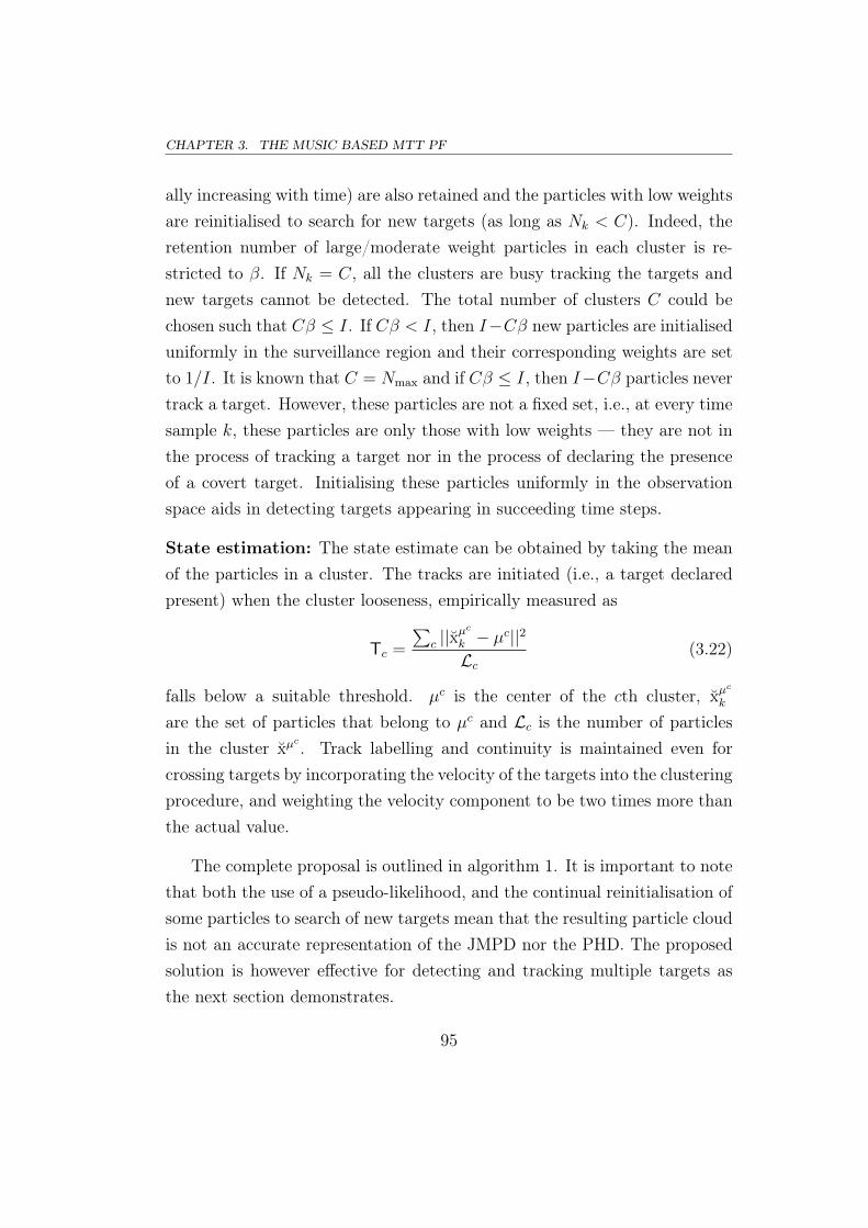
CHAPTER 3. THE MUSIC BASED MTT PF
ally increasing with time) are also retained and the particles with low weightsare reinitialised to search for new targets (as long as Nk < C). Indeed, theretention number of large/moderate weight particles in each cluster is re-stricted to β. If Nk = C, all the clusters are busy tracking the targets andnew targets cannot be detected. The total number of clusters C could bechosen such that Cβ ≤ I. If Cβ < I, then I−Cβ new particles are initialiseduniformly in the surveillance region and their corresponding weights are setto 1/I. It is known that C = Nmax and if Cβ ≤ I, then I−Cβ particles nevertrack a target. However, these particles are not a fixed set, i.e., at every timesample k, these particles are only those with low weights — they are not inthe process of tracking a target nor in the process of declaring the presenceof a covert target. Initialising these particles uniformly in the observationspace aids in detecting targets appearing in succeeding time steps.
State estimation: The state estimate can be obtained by taking the meanof the particles in a cluster. The tracks are initiated (i.e., a target declaredpresent) when the cluster looseness, empirically measured as
Tc =
∑c ||x
µc
k − µc||2
Lc(3.22)
falls below a suitable threshold. µc is the center of the cth cluster, xµc
k
are the set of particles that belong to µc and Lc is the number of particlesin the cluster xµ
c . Track labelling and continuity is maintained even forcrossing targets by incorporating the velocity of the targets into the clusteringprocedure, and weighting the velocity component to be two times more thanthe actual value.
The complete proposal is outlined in algorithm 1. It is important to notethat both the use of a pseudo-likelihood, and the continual reinitialisation ofsome particles to search of new targets mean that the resulting particle cloudis not an accurate representation of the JMPD nor the PHD. The proposedsolution is however effective for detecting and tracking multiple targets asthe next section demonstrates.
95

3.6. REGULATED CLUSTERING
Algorithm 1 {xik, wik}Ii=1 = PF[{xik−1, wik−1}Ii=1, zk]
1. Prediction: xik ∼ q(.|xik−1, zk), i = 1, ..., I
2. Weight update: wik = wik−1
SMU(xik) p(xik|xik−1)
q(.|xik−1,z1:k), i = 1, ..., I
3. Normalise the weights: wik =wik∑Ij=1 w
jk
4. Clustering: {xc,ik , wc,ik }Ii=1
clustering←−−−−− {xik, wik}Ii=1 ; c ∈ χ = {1, ..., C}
5. Soft resample: {xc,ik , wc,ik }Ii=1
resample←−−−−− {xc,ik , wc,ik }Ii=1
6. Cluster regulation:for c = 1, ..., C doObtain the subset of the weighted particles that belong to the cluster c,i.e., {xlk, wlk}
Lcl=1 ∈ {x
c,ik , w
c,ik }Ii=1 : c = c
if Lc ≥ β then{ξlk}
cβl=(c−1)β+1 = {xlk}
βl=1
{Ψ lk}cβl=(c−1)β+1 = {wlk}
βl=1
else{ξlk}
cβl=(c−1)β+1 = {xlk}
Lcl=1 ∪ {x
jk}
β−Lcj=1 where xjk ∼ U(.)
{Ψ lk}cβl=(c−1)β+1 = {wlk}
Lcl=1 ∪ {w
jk}
β−Lcj=1 where wjk = 1/I
end ifend forif Cβ < I thenInitialise new particles and their weightsξjk ∼ U(.), j = Cβ + 1, ..., I
Ψ jk = 1/I, j = Cβ + 1, ..., I
end if
7. Normalise the weights: Φik = 1∑Ij=1 Ψ
jk
, i = 1, ..., I
8. The output: {xik, wik}Ii=1 = {ξik, Φik}Ii=1
96

CHAPTER 3. THE MUSIC BASED MTT PF
3.7 Simulation results
All the simulations presented here consider acoustic sensing in a 2D envi-ronment which includes a 1 second reverberation time for 60 dB decay. Thestate of the target is defined as xk = (x, y, vx, vy)
T where x, y are the posi-tions and vx, vy are the velocities along the x, y-axis. xk evolves with timein accordance to a Markov model in which the position is updated using aconstant velocity (CV) model and the velocity is updated using a randomwalk (RW). This process is described as
xk =
1 0 T 0
0 1 0 T
0 0 1 0
0 0 0 1
xk−1 + qk−1 (3.23)
where the duration between two observations is T = 1s and the process noiseis qk−1 ∼ N (0, Q). Q is the uncorrelated covariance matrix with a varianceof 0.5 along each dimension. The sensor signals are obtained using the modeldescribed in (3.1). The sensor noise vector is vk ∼ CN (0, R) where R is adiagonal with a variance of σ2 = 0.1 corresponding to each sensor.
Demonstration
Firstly, Fig. 3.3 demonstrates the proposed filter operation for tracking sin-gle/multiple and appearing/disappearing targets. It can be seen that thefilter quickly locks onto the targets as they appear, thereby initialising thetracks. If a target disappears, the particles tracking it disperse, thereby re-moving the track and these particles then start to search for new targets.
In Fig. 3.4 the particle evolution for the scenario described in Fig. 3.3 isshown. Here, only the particle clusters whose exp(−Tc) exceed 0.75 are con-sidered for the filter estimate and shown in Fig. 3.4. The use of the Markovtransition prior as the importance distribution is known to be sub-optimal.
97

3.7. SIMULATION RESULTS
1 2 3 4 51
1.5
2
2.5
3
3.5
4
4.5
5
x−position [m]
y−
po
sitio
n [
m]
Target 1 (1
,50)
Target 2
(11,35)
Target 3 (26,40)
Target 4 (31,50)
Target 5 (30,50)
Ground truth
Filter estimate
Figure 3.3: This figure shows the ground truth and the filter estimates. Targets move in a4×4 2D space. A linear array of 5 sensors at an offset of 10m from grid of target movementis used. The number of particles I = 5000. At k = 0, the particles are initialised uniformlyin the surveillance region. The number of clusters is C = 10, the maximum number ofparticles in a cluster is β = 480, the cluster looseness threshold to initiate and removetracks is exp(−Tc) = 0.75, the frequency of operation is f = 4KHz and the propagationvelocity is ν = 1500m/s. The SNR is 27dB. The filter runs for 50 time steps. The text inthe figure denotes – Target #(appears at # time step, disappears at # time step). Thedirection in which each target moves is denoted using arrows.
An importance distribution leveraging the current observation has been pro-posed for the joint filter [71, 127, 220] and the PHD filter [180]. It may bethat the proposed MTT PF could be enhanced using an improved impor-tance distribution. Nevertheless, it can be seen in Fig. 3.3 and Fig. 3.4 thattrack initialisation and deletion are conducted very effectively.
98
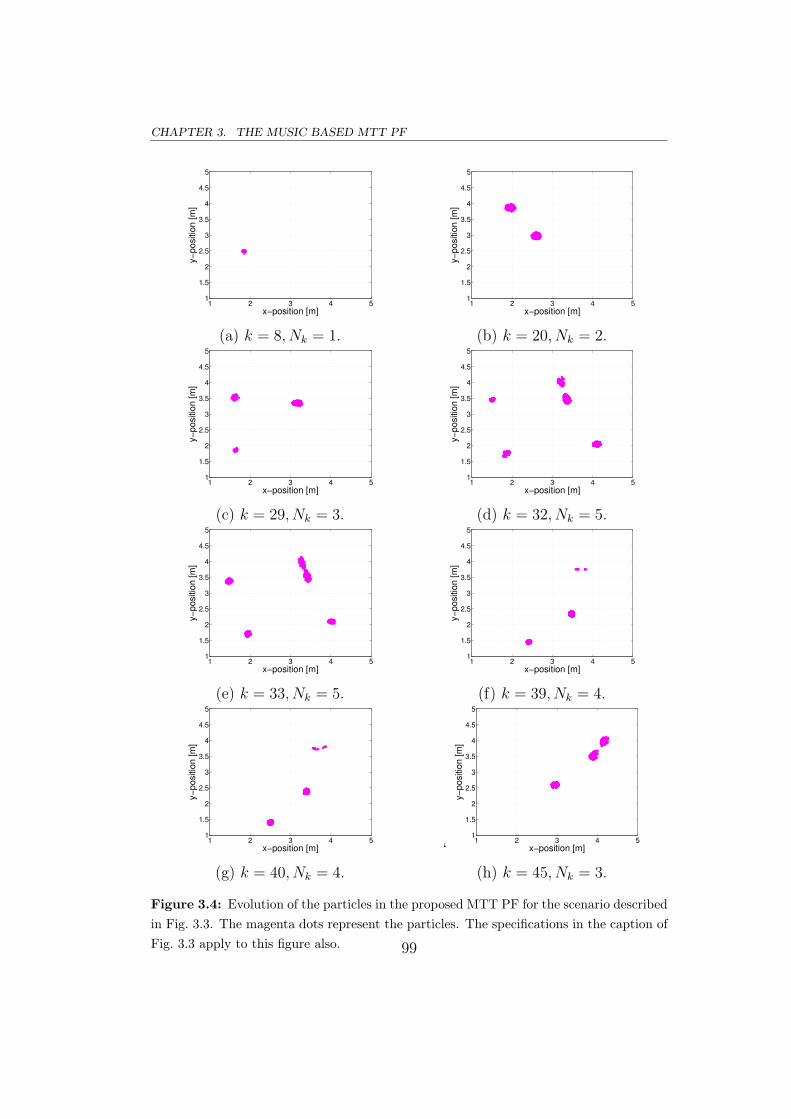
CHAPTER 3. THE MUSIC BASED MTT PF
1 2 3 4 51
1.5
2
2.5
3
3.5
4
4.5
5
x−position [m]
y−
po
sitio
n [m
]
(a) k = 8, Nk = 1.
1 2 3 4 51
1.5
2
2.5
3
3.5
4
4.5
5
x−position [m]
y−
po
sitio
n [m
]
(b) k = 20, Nk = 2.
1 2 3 4 51
1.5
2
2.5
3
3.5
4
4.5
5
x−position [m]
y−
positio
n [m
]
(c) k = 29, Nk = 3.
1 2 3 4 51
1.5
2
2.5
3
3.5
4
4.5
5
x−position [m]
y−
positio
n [m
]
(d) k = 32, Nk = 5.
1 2 3 4 51
1.5
2
2.5
3
3.5
4
4.5
5
x−position [m]
y−
positio
n [m
]
(e) k = 33, Nk = 5.
1 2 3 4 51
1.5
2
2.5
3
3.5
4
4.5
5
x−position [m]
y−
positio
n [m
]
(f) k = 39, Nk = 4.
1 2 3 4 51
1.5
2
2.5
3
3.5
4
4.5
5
x−position [m]
y−
positio
n [m
]
(g) k = 40, Nk = 4.‘
1 2 3 4 51
1.5
2
2.5
3
3.5
4
4.5
5
x−position [m]
y−
positio
n [m
]
(h) k = 45, Nk = 3.
Figure 3.4: Evolution of the particles in the proposed MTT PF for the scenario describedin Fig. 3.3. The magenta dots represent the particles. The specifications in the caption ofFig. 3.3 apply to this figure also. 99

3.7. SIMULATION RESULTS
Fig. 3.4 shows only the particles belonging to the clusters in which exp(−Tc) >0.75. However, as long as Nk < C, the filter has particles associated withthe other clusters that are not near the targets. These clusters are free tosearch for new targets and hence the particles belonging to these clustersare distributed uniformly in the entire observation space. This is illustratedin Fig. 3.5. The figure shows a stem plot of the MUSIC pseudo-weights ofall the particles after the soft resampling stage in algorithm 1. The figurecorresponds to the 29th time step at which Nk = 3. For ease of visualisation,I = 1000, C = 4, β = 200. It can be seen that three clusters keep track of thethree targets. Moreover, these clusters have gained more replications sincethey are near the targets. It can also be observed that the particles belongingto the fourth cluster and the remaining I − Cβ = 200 particles are free to
1
2
3
4
5 1
2
3
4
50
2000
4000
y−position [m]
x−position [m]
MU
SIC
pse
ud
o−
we
igh
ts
Figure 3.5: The MUSIC pseudo-weights of the particles for the MTT scenario shown inFig. 3.3 at k = 29. The specifications in the caption of Fig. 3.3 apply to this figure also.
100
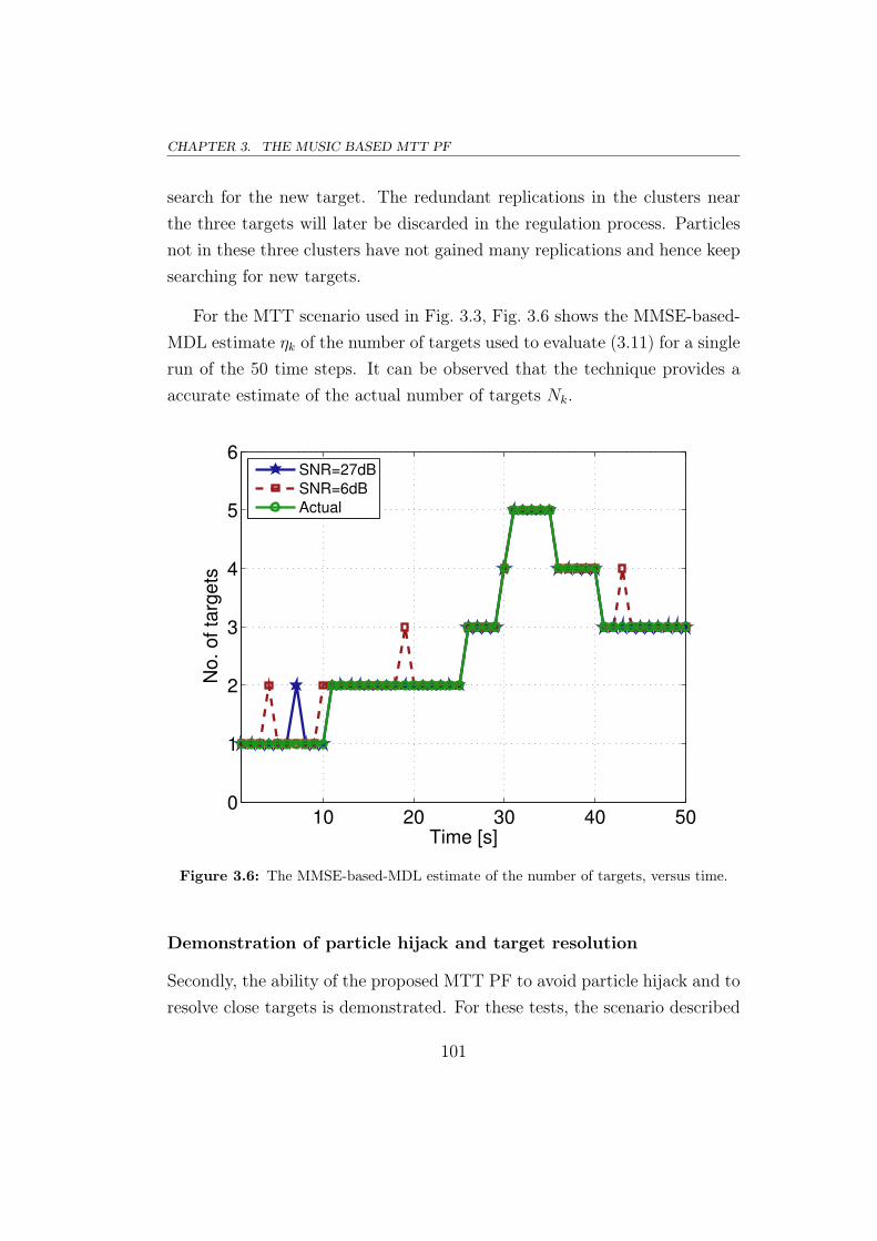
CHAPTER 3. THE MUSIC BASED MTT PF
search for the new target. The redundant replications in the clusters nearthe three targets will later be discarded in the regulation process. Particlesnot in these three clusters have not gained many replications and hence keepsearching for new targets.
For the MTT scenario used in Fig. 3.3, Fig. 3.6 shows the MMSE-based-MDL estimate ηk of the number of targets used to evaluate (3.11) for a singlerun of the 50 time steps. It can be observed that the technique provides aaccurate estimate of the actual number of targets Nk.
10 20 30 40 500
1
2
3
4
5
6
Time [s]
No
. o
f ta
rge
ts
SNR=27dB
SNR=6dB
Actual
Figure 3.6: The MMSE-based-MDL estimate of the number of targets, versus time.
Demonstration of particle hijack and target resolution
Secondly, the ability of the proposed MTT PF to avoid particle hijack and toresolve close targets is demonstrated. For these tests, the scenario described
101
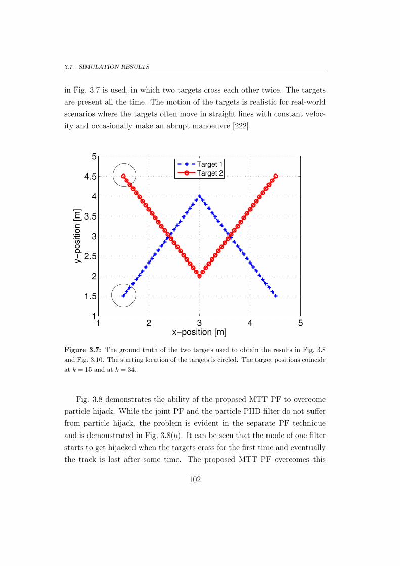
3.7. SIMULATION RESULTS
in Fig. 3.7 is used, in which two targets cross each other twice. The targetsare present all the time. The motion of the targets is realistic for real-worldscenarios where the targets often move in straight lines with constant veloc-ity and occasionally make an abrupt manoeuvre [222].
1 2 3 4 51
1.5
2
2.5
3
3.5
4
4.5
5
x−position [m]
y−
po
sitio
n [
m]
Target 1
Target 2
Figure 3.7: The ground truth of the two targets used to obtain the results in Fig. 3.8and Fig. 3.10. The starting location of the targets is circled. The target positions coincideat k = 15 and at k = 34.
Fig. 3.8 demonstrates the ability of the proposed MTT PF to overcomeparticle hijack. While the joint PF and the particle-PHD filter do not sufferfrom particle hijack, the problem is evident in the separate PF techniqueand is demonstrated in Fig. 3.8(a). It can be seen that the mode of one filterstarts to get hijacked when the targets cross for the first time and eventuallythe track is lost after some time. The proposed MTT PF overcomes this
102

CHAPTER 3. THE MUSIC BASED MTT PF
hijack problem by virtue of limiting the cluster size to β and reinitialisingthe redundant lower weight particles.
1 2 3 4 51
2
3
4
5
x−position [m]
y−
positio
n [m
]
(a) Separate filter.
1 2 3 4 51
2
3
4
5
x−position [m]
y−
positio
n [m
](b) Proposed filter.
Figure 3.8: Evolution of the particles in various PF’s with time for the scenario describedin Fig. 3.7. A linear array of 5 sensors with an offset of 10m from the grid of targetmovement is used. f = 4KHz, ν = 1500m/s and SNR= 27dB. The particles are initialiseduniformly in the surveillance region and a burn-in time of 4s is applied before starting theplot. For the separate filter technique, two filters, each using 1000 particles, are initialised.For the proposed filter, I = 1000, C = 2, β = 500 and exp(−Tc) = 0.75.
Now the ability of the proposed MTT PF to resolve close targets bet-ter than that of the PHD filter is demonstrated. In view of the fact thatthe latter cannot operate directly on the array data, the sensor signals arefirst converted into the minimum variance distortionless response (MVDR)beamformer image [244] which is then thresholded to generate the observa-tion feed. In the proposed method, the observations are the sensor signals.Fig. 3.9 illustrates the super-resolution property of MUSIC when comparedwith the beamformer image. The PF implementation for the ground truthin Fig. 3.7 is illustrated in Fig. 3.10 and it can be seen that the proposedmethod resolves the targets for a longer duration. At the first crossing atk = 15, the PHD filter resolved the targets only until k = 12 while the pro-posed filter until k = 14. Before the second crossing at k = 34, the PHDfilter resolved the targets only until k = 31 while the proposed filter until
103

3.7. SIMULATION RESULTS
k = 33. The PHD filter resolution is dependent on how the beamformerimage is thresholded — a low threshold deteriorates resolution but a highthreshold could degrade the track accuracy at low SNR.
(a) MVDR beamformer image. (b) MUSIC image.
Figure 3.9: Beamformer and MUSIC outputs with two closely spaced targets.
1 2 3 4 51
2
3
4
5
x−position [m]
y−
positio
n [m
]
(a) Particle-PHD filter.
1 2 3 4 51
2
3
4
5
x−position [m]
y−
positio
n [m
]
(b) Proposed filter.
Figure 3.10: Evolution of the particles with time. For the proposed filter, the specifica-tions in the caption of Fig. 3.8 apply to this figure also. For the particle-PHD filter; (i)detection probability pD = 0.95, (ii) target birth is not considered, (iii) thresholding isdone at 50% of the maximum peak in the beamformer image, (iv) 1000 particles are used,and (v) targets are separated using k-means clustering [169].
104

CHAPTER 3. THE MUSIC BASED MTT PF
Evaluation of track accuracy
Thirdly, the accuracy of the proposed technique is evaluated by plotting thetarget position root mean square (rms) error for different SNR levels. Thisis shown in Fig. 3.11 and it can be seen that the proposed technique is moreaccurate than the particle-PHD filter. The performance advantage of theproposed filter as against the PHD filter can be attributed to the fact thatthe former operates directly on the sensor signals while the latter undergoesinformation loss due to the use of an image processing stage. As the SNRreduces, the false alarms in the finite set measurement feed for the PHDfilter increase causing degradation of the accuracy of the track. On the otherhand, the separate filter and the joint filter techniques that operate with thetrue likelihood function in (3.3) exhibit better accuracy than the proposedMTT PF and the particle-PHD filter.
Evaluation of computational complexity
Fourthly, the computational complexity of the proposed technique is evalu-ated by plotting the computational time taken to evaluate one time step forvarying numbers of particles. This is shown in Fig. 3.12. It can be observedthat the proposed technique requires fewer computational resources than theothers because it uses only I particles (in the domain of one target) that areclustered amongst the two targets. The separate PF technique uses 2I parti-cles, i.e., I particles for each target, and the multi-dimensional joint PF usesI particles of double the dimension. In the particle-PHD filter, the majorityof the time is consumed evaluating the beamformer image for the entire gridto obtain the finite set measurement feed for the filter. As mentioned in thecaption of Fig. 3.11, the number of pixels in the beamformer image is 1681
and hence the filter is slower if I / 1700.
105

3.7. SIMULATION RESULTS
5 10 15 20 25 30 35 400
0.2
0.4
0.6
0.8
1
SNR [dB]
rms e
rro
r [m
]
Separate filter
Joint filter
Particle−PHD
MUSIC−PF
Figure 3.11: rmse error of various PFs versus the SNR for the scenario described inFig. 3.7. A linear array of 5 sensors with an offset of 10m from the grid of target movementis used. f = 4KHz and ν = 1500m/s. It is assumed that the knowledge about the numberof targets is available. Hence, for the separate filter technique, two filters, each using1000 particles are initialised. The joint filter uses 1000 particles that operate in the statespace of two targets. For the particle-PHD filter, the beamformer image is evaluated overthe observation space with a resolution of 0.1m. Therefore, the total number of pixels inthe beamformer image are 1681. During the particle-PHD filter implementation; a) thedetection probability pD = 0.95, b) target birth is not considered, c) thresholding is doneat 50% of the maximum peak in the beamformer image, and d) 1000 particles are used. Toobtain state estimates, the k-means clustering approach of [169] is used. For the proposedfilter, I = 1000, C = 2, β = 500 and exp(−Tc) = 0.75. No burn-in time is considered.The results are averaged over 30 scenarios, each comprising 50 time steps.
106

CHAPTER 3. THE MUSIC BASED MTT PF
102
103
100
101
No. of particles
Com
puta
tional tim
e [s]
Separate filter
Joint filterParticle−PHD
MUSIC−PF
Figure 3.12: Computational time for one time step of various PFs versus the number ofparticles. The specifications in the caption of Fig. 3.11 apply to this figure, except thatnow, I is varied and the SNR=27dB. The results are averaged over 30 scenarios, eachcomprising 50 time steps.
Demonstration of track continuity
Finally, the track continuity in the proposed MTT PF is demonstrated. Asproposed in section 3.6.3, the track continuity is maintained by incorporatingthe velocity into the clustering procedure with a weighting that is twice itsactual value. For a three target case, Fig. 3.13 shows the track continuity inthe proposed filter for crossing targets using colored particle clusters. It canbe seen that the filter successfully maintains the track of the crossing targets.However, it would be difficult to maintain tracks if two targets travel togetherfor some duration and then seperate with opposite velocities.
107

3.7. SIMULATION RESULTS
−30 −20 −10 0 10 20 30 40
10
15
20
x−position[m]
y−
positio
n[m
]
−30 −20 −10 0 10 20 30 40
10
15
20
x−position[m]
y−
positio
n[m
]
−30 −20 −10 0 10 20 30 40
10
15
20
x−position[m]
y−
positio
n[m
]
−30 −20 −10 0 10 20 30 40
10
15
20
x−position[m]
y−
positio
n[m
]
−30 −20 −10 0 10 20 30 40
10
15
20
x−position[m]
y−
positio
n[m
]
Figure 3.13: Particle evolution in the proposed MTT PF with time. Here I = 6000,C = 3 and β = 2000. The figures from top to bottom correspond to time steps k =
9, 10, 11, 12, 15 respectively. The blue crossed line is the ground truth. The red solid lineis the filter estimate. The three clusters are represented in different colors. The greenstars depict a linear array of 10 sensors.
108

CHAPTER 3. THE MUSIC BASED MTT PF
3.8 Conclusion and summary
This chapter addressed the problem of Bayesian MTT using phased sensorarrays under the PF framework. State-of-the-art approaches to this probleminclude the separate filter approach which suffers from filter hijack, the jointapproach which suffers from high computational complexity and the PHD fil-ter [26] which suffers from the inability to operate directly on phased sensorarray signals. This chapter proposed MUSIC based MTT PF, the key inno-vation of which is to use for the likelihood function, a function which has asits domain, the state space of a single target. The MUSIC pseudo-spectrumis such a function, and has not previously been used in this context. The par-ticle hijack problem is overcome using regulated clustering. This work is thefirst to propose soft resampling for cluster regulation — a novel mechanismthat provided means for initialising new particles that account for appearingtargets. The advantages of the developed filter are; a) lower computationalcomplexity by virtue of operating in the single target space, b) better accu-racy by virtue of operating more directly on sensor array signals, c) effectiveseperation of close targets by virtue of the super resolution property of MU-SIC, and d) avoidance of particle hijack by virtue of regulated clustering. Thevalidity and the efficacy of the technique were illustrated through a simulatedstudy. Referring back to section 1.3.1 of chapter 1, it can be stated that theresearch goal 1 that aims to overcome problems 1,2 has been successfullyachieved by the proposed MUSIC based MTT PF. Further evaluation of theperformance of this algorithm is included in section 4.6.1 of the next chapter.
109

3.8. CONCLUSION AND SUMMARY
110

4The MUSIC based MeMBer filter
Bayesian filtering (Ch. 2)
Bayesian MTT for array processing
MUSIC basedMTT PF (Ch. 3)
MUSIC basedMeMBer filter (Ch. 4)
Particle filtering
Soft resampling(Ch. 5)
KS statistic to measurePF performance (Ch. 5)
BBBayesian filtering [35] provides a rigorous mathematical framework formultiple target tracking (MTT) using phased sensor arrays — an applicationof primary interest to this dissertation. However, Bayes’ filtering involveshigh dimensional integration which makes the process computationally in-tractable [45]. This intractability is overcome using approximate solutions.The Bayes’ approximation which is central to this thesis is the particle filter(PF) [21] described in section 2.5 of chapter 2.
The theoretically accurate approach to Bayesian MTT is the joint fil-ter approach [44, 124]. However, the joint PF is computationally expensive[232] and this drawback restricts its use for tracking many targets. The high
111

4.1. RELATED WORK
computational complexity suffered by the joint filter has been successfullyovercome using the random finite set (RFS) filters [179] — the probabil-ity hypothesis density (PHD) filter [26, 32, 167] and the multi-target multi-Bernoulli (MeMBer) filter [31, 32, 196, 198, 208, 209]. The major drawbackin RFS filters, as identified in problem 2 of section 1.3.1 in chapter 1, isthat they do not possess the mathematical framework to operate directly onphased array data and consequently the array data has to be converted intoa suitable format. This conversion leads to high information and resolutionloss. The research goal 2 in section 1.3.1 of chapter 1 aims to explore thepossibility and develop a method of operating either the PHD or the MeM-Ber filters directly on phased sensor array signals. This chapter presents thedevelopment of such a method and illustrates its efficacy.
The chapter is organised as follows: The drawbacks and related work instate-of-the-art RFS filters are outlined in section 4.1. After stating the moti-vation in section 4.2, the phased sensor array model and the particle-MeMBerfilter for image observations are revisited in section 4.3 and section 4.4 respec-tively. This is followed by the proposed method in section 4.5, the simulationresults in section 4.6 and the concluding remarks in section 4.7.
4.1 Related work
The class of Bayesian sub-optimal filters developed for tracking many targetsare the RFS filters [233] — the PHD [26] and the MeMBer [31, 32] filters. ThePHD filter described in section 2.6 of chapter 2 operates by approximatingthe joint multi-target probability distribution (JMPD) ((2.13) in section 2.3.2of chapter 2) by its first moment. The PF implementation of the PHD filtercan be found in [161, 162, 164]. The MeMBer filter [198, 209] described insection 2.7 of chapter 2 approximates the JMPD using its multi-BernoulliRFS parameters. The PF implementation of the MeMBer filter can be foundin [31, 33, 49, 196]. The PHD and MeMBer filters are derived under the RFStheoretic framework [34, 233] that allows them to operate in the dimension-
112

CHAPTER 4. THE MUSIC BASED MEMBER FILTER
ality of a single target, i.e., their complexity does not increase exponentiallywith the number of targets. However, since the filters are sub-optimal, theirperformance is poor in many situations [266, 267], for example, in high noisescenarios [161].
The major impediment in RFS filtering, as mentioned in section 3.1 ofchapter 3, is that the observation feed to the filters can only be a finite setof noisy point target measurements [32], thereby impeding the direct use ofphased sensor array data. This drawback is only partially overcome when theMeMBer filter has been extended to image observations [49, 196]. To date,the RFS filters do not provide a suitable mathematical formalism to evaluatethe likelihood function for phased array data, because these filters operatein the dimensionality of a single target, while the phased array data requiresa joint state hypothesis to evaluate the likelihood. In the PHD filter, thisproblem is usually bypassed by first converting the array data into a beam-former image [50, 189, 191], and then pre-processing the image [192] to obtainthe measurement feed. The “MeMBer filter for image observations” does notrequire image pre-processing, but still necessitates the conversion of the sen-sor array data into a image. A closely related work in [268, 269] deals withsuper-positional sensors that generate a “single measurement” from multipletargets. However, this single measurement was considered to be a point esti-mate of the targets rather than a signal. This still requires the array data tobe converted to a beamformer image. These conversions lead to substantialinformation and resolution loss.
4.2 Motivation
This thesis proposes that the formulation in the “MeMBer filter for imageobservations” provides a possibility to operate the filter more directly onthe sensor array data. The aim now is to adapt the MeMBer filter for imageobservations to phased sensor array observations. The key idea for this adap-tion is to find a function (generated using the array data), whose domain is
113

4.3. PHASED SENSOR ARRAY MODEL
the domain of a single target, and which can act as a proxy to the MeM-Ber update equation without changing its formulation. The MUltiple SIgnalClassification (MUSIC) pseudo-spectrum [57] is such a function. MUSIC isone of what are called “super-resolution techniques.” This work proposes touse MUSIC as the pseudo-likelihood in the MeMBer filter for image obser-vations.
The MUSIC based MTT PF proposed in chapter 3 compared favourablywith the PHD filter and the comparison with the MeMBer filter has beendeferred until this chapter. In this chapter, the comparative analysis withthe conventional PHD and MeMBer filters, the previously proposed MU-SIC based MTT PF, and the MUSIC based MeMBer filter of this chapter ispresented.
4.3 Phased sensor array model
Here, the phased sensor array observation model [38] (previously presentedin section 3.3 of chapter 3) is briefly described. The observation model isformulated as
zk = Aksk + vk (4.1)
where zk is the vector of sensor signals, sk is the signal vector and the noisevector vk ∼ CN (0, R). Ak is a M×Nk steering matrix where M is the numberof sensors and Nk is the number of targets at time k. For this sensing model,the likelihood equation is
p(zk|Ak, sk) =1
πM det(R)exp(− (zk − Aksk)H R−1 (zk − Aksk)
)(4.2)
where (.)H denotes Hermitian transpose. The PHD and MeMBer filters donot possess a framework to evaluate (4.2). This non-provision can be by-passed using beamformer image models [50, 189, 191, 192]. The proposal inthis chapter is based on the idea that using MUSIC1 as a proxy for the likeli-
1It is known from the MUSIC based MTT PF in chapter 3 that MUSIC allows theparticles to operate in the space of a single target, a requisite for the MeMBer filter.
114

CHAPTER 4. THE MUSIC BASED MEMBER FILTER
hood provides a framework to feed the sensor array data as an observation tothe MeMBer filter (for image observations) without changing its formulation.Moreover, the super resolution property of MUSIC aids in separating veryclose targets. The objective now is to adapt the MeMBer filter for imageobservations to phased sensor array signals zk obtained from (4.1).
4.4 The particle-MeMBer filter for image data
The operation of the MeMBer filter for image data [49, 196, 208, 211, 214]was described in section 2.7.3 of chapter 2. Here its particle implementationis briefly described. The filter is derived and explained in more detail in[49, 196]. The proposal of adapting the MeMBer filter to array data thenbuilds on the formulation provided in this section.
In MeMBer filtering, the uncertainty in the knowledge of the numberof targets and their states is modelled using a multi-Bernoulli RFS Ξ. Amulti-Bernoulli RFS Ξk at time k can be considered as the union of a fixednumber of independent Bernoulli sets. The nth Bernoulli set in Ξk is de-scribed by its a) existence probability εnk , and b) probability density function(pdf) pn(xk). In the particle approach, the pdf is approximated using a set ofI weighted particles, i.e., pn(xk) is now represented by the weighted sampleset {xn,ik , w
n,ik }Ii=1.
The particle-MeMBer filter recursion is as follows (the explanation providedin section 2.7.3 of chapter 2 is directly applicable to the particle-MeMBerfilter): If the particle-MeMBer approximation to the posterior at time k − 1
is available and represented by
p(Xk−1|zk−1) u{εnk−1, {x
n,ik−1, w
n,ik−1}
Ii=1
}Nk−1
n=1(4.3)
115

4.4. THE PARTICLE-MEMBER FILTER FOR IMAGE DATA
where we define u to mean “is represented by,” then the particle-MeMBerapproximation to the Bayes’ prediction is represented by
p(Xk|z1:k−1) u {εnk , {xn,ik , w
n,ik }
Ii=1}
Nkn=1
u {εnP,k, {xn,iP,k, w
n,iP,k}
Ii=1}
Nk−1
n=1 ∪ {εnB,k, {xn,iB,k, w
n,iB,k}
Ii=1}
NB,kn=1
(4.4)
The multi-Bernoulli RFS {εnP,k, {xn,iP,k, w
n,iP,k}Ii=1}
Nk−1
n=1 in (4.4) contains theBernoulli parameters (or target hypotheses) that persist from time k − 1 totime k. For n = 1, ..., Nk−1, the Bernoulli parameters are predicted accordingto
εnP,k = εnk−1
I∑i=1
wn,ik−1 pS(xn,ik−1) (4.5)
xn,iP,k ∼ q(.|xn,ik−1, zk) = p(xn,iP,k|xn,ik−1) ; i = 1, ..., I (4.6)
wn,iP,k =wn,ik−1 pS(xn,ik−1)∑Il=1 w
n,lk−1 pS(xn,lk−1)
; i = 1, ..., I (4.7)
where pS(.) is the survival probability of the particle.
In (4.5), εnP,k is the existence probability that the nth persisting BernoulliRFS contains an actual target; if the survival probability is a constant valuepS, then εnP,k is obtained by directly scaling the existence probability εnk−1
of the Bernoulli RFS at the previous time step with pS (since the particleweights sum to one). In (4.6), the particles that represent the pdf at timek − 1 are propagated to time k by drawing a new set of particles from theMarkov transition prior. In (4.7), the weights of the predicted particles sur-vive from time k− 1 to k in accordance to the particle survival probabilities.These weights are then normalised.
The multi-Bernoulli RFS {εnB,k, {xn,iB,k, w
n,iB,k}Ii=1}
NB,kn=1 in (4.4) contains the
multi-Bernoulli parameters for the NB,k new-born targets at time k, whereNB,k ∼ Pois(λB). The new particles are initialised near regions of target ap-pearance and the existence probabilities are set accordingly. If the informa-tion about regions of target appearance is not available, then εnB,k ∼ U(0, 1],
116

CHAPTER 4. THE MUSIC BASED MEMBER FILTER
and for i = 1, ..., I, xn,iB,k ∼ U(.) and wn,iB,k = 1/I.
Once the new image observation zk and the predicted particle-MeMBer pa-rameters {εnk , {x
n,ik , w
n,ik }Ii=1}
Nkn=1 are available, the posterior at time k can be
approximated [49] using the updated Bernoulli parameters as
p(Xk|z1:k) u {εnk , {xn,ik , w
n,ik }
Ii=1}
Nkn=1 (4.8)
where
εnk =εnk∑I
i=1 wn,ik szk(x
n,ik )
1− εnk + εnk∑I
i=1 wn,ik szk(x
n,ik )
(4.9)
wn,ik =wn,ik szk(x
n,ik )∑I
l=1 wn,lk szk(x
n,lk )
(4.10)
Here, (4.9) gives the updated existence probability of the nth Bernoulli RFS(its functionality was discussed in Fig. 2.8 of section 2.7.3 in chapter 2).(4.10) gives the updated particle weights; this is obtained using a PF up-date step — by multiplying the predicted weights with the likelihood valueof the particles. The weights are then normalised. The updated particles{{xn,ik }Ii=1}
Nkn=1 in (4.8) are obtained by resampling the particles (based on
their updated weights) in each predicted Bernoulli set separately.
The state estimate is the mean of all the particles belonging to a Bernoulliset. If the distance between the estimates of two Bernoulli sets is closerthan a threshold Tmerge, their tracks are merged [32]. The state estimates ofBernoulli sets whose existence probability exceeds a threshold Tprune are onlyreported.
The term szk(xn,ik ) in (4.9) and (4.10) is the likelihood ratio of the ith
particle in the nth predicted Bernoulli set and its formulation was given in(2.107) of section 2.7.2 in chapter 2. Using the image observation modeldescribed2 in Ch. 11 of [56] in which the signal and noise components fol-low a Gaussian distribution, the szk(x
n,ik ) in (2.107) can be written up to a
2The complete model is presented further in section 5.6.1 of chapter 5.
117

4.5. THE MUSIC BASED MEMBER FILTER
normalising constant as (shown in (2.111))
szk(xn,ik ) =
∏(x,y)∈R0(xn,ik )
exp
(−γ
(x,y)
xn,ik(γ
(x,y)
xn,ik− 2z
(x,y)k )
2σ2
)(4.11)
Here, zk is the received image. The hypothesis measure γxn,ik(also a image)
is the intensity contribution of the particle xn,ik and is constructed from theimage observation model considering the absence of noise. The particle xn,ikilluminates a region R0(x
n,ik ) of the image, i.e., the target hypothesis xn,ik will
illuminate a set of pixels, the centers (x, y) of which will lie within the regionof illuminance R0(x
n,ik ). This was illustrated in Fig. 2.7 in which a target
at position (40, 40) illuminates a set R0(.) of pixels within the frame. Forimage models, the set of pixels with centers (x, y) ∈ R0(x
n,ik ) required to
evaluate (4.11) is usually fixed and known in advance. If this informationis not available, then R0(.) can be obtained by thresholding γxn,ik
using anillumination threshold Il which is usually a certain proportion of the peak inthe image γxn,ik
. Then the likelihood szk(.) is obtained by taking the productof the exponential at each of these pixels. Note that (4.11) is computed forall the INk particles in the predicted multi-Bernoulli set.
4.5 The MUSIC based MeMBer filter
The non-Bayesian MUSIC algorithm for target localisation has been de-scribed in section 3.5.1 of chapter 3 and will not be repeated here. In thiswork, the proposal is to use the MUSIC value as a pseudo-likelihood for theparticle [270]. Hence, the proposed MUSIC based particle-MeMBer filter op-eration is just as described in section 4.4, except that (4.9) and (4.10) arenow computed according to
εnk =εnk∑I
i=1 wn,ik SMU(xn,ik )
1− εnk + εnk∑I
i=1 wn,ik SMU(xn,ik )
(4.12)
wn,ik =wn,ik SMU(xn,ik )∑Il=1 w
n,lk SMU(xn,lk )
(4.13)
118
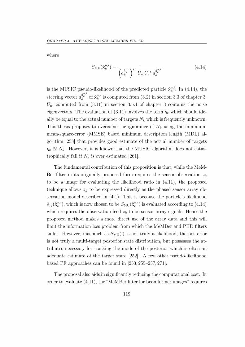
CHAPTER 4. THE MUSIC BASED MEMBER FILTER
where
SMU(xn,ik ) =1(
axn,ikk
)HUn UH
n axn,ikk
(4.14)
is the MUSIC pseudo-likelihood of the predicted particle xn,ik . In (4.14), the
steering vector axn,ikk of xn,ik is computed from (3.2) in section 3.3 of chapter 3.
Un, computed from (3.11) in section 3.5.1 of chapter 3 contains the noiseeigenvectors. The evaluation of (3.11) involves the term ηk which should ide-ally be equal to the actual number of targets Nk which is frequently unknown.This thesis proposes to overcome the ignorance of Nk using the minimum-mean-square-error (MMSE) based minimum description length (MDL) al-gorithm [258] that provides good estimate of the actual number of targetsηk u Nk. However, it is known that the MUSIC algorithm does not catas-trophically fail if Nk is over estimated [261].
The fundamental contribution of this proposition is that, while the MeM-Ber filter in its originally proposed form requires the sensor observation zk
to be a image for evaluating the likelihood ratio in (4.11), the proposedtechnique allows zk to be expressed directly as the phased sensor array ob-servation model described in (4.1). This is because the particle’s likelihoodszk(x
n,ik ), which is now chosen to be SMU(xn,ik ) is evaluated according to (4.14)
which requires the observation feed zk to be sensor array signals. Hence theproposed method makes a more direct use of the array data and this willlimit the information loss problem from which the MeMBer and PHD filterssuffer. However, inasmuch as SMU(.) is not truly a likelihood, the posterioris not truly a multi-target posterior state distribution, but possesses the at-tributes necessary for tracking the mode of the posterior which is often anadequate estimate of the target state [252]. A few other pseudo-likelihoodbased PF approaches can be found in [253, 255–257, 271].
The proposal also aids in significantly reducing the computational cost. Inorder to evaluate (4.11), the “MeMBer filter for beamformer images” requires
119
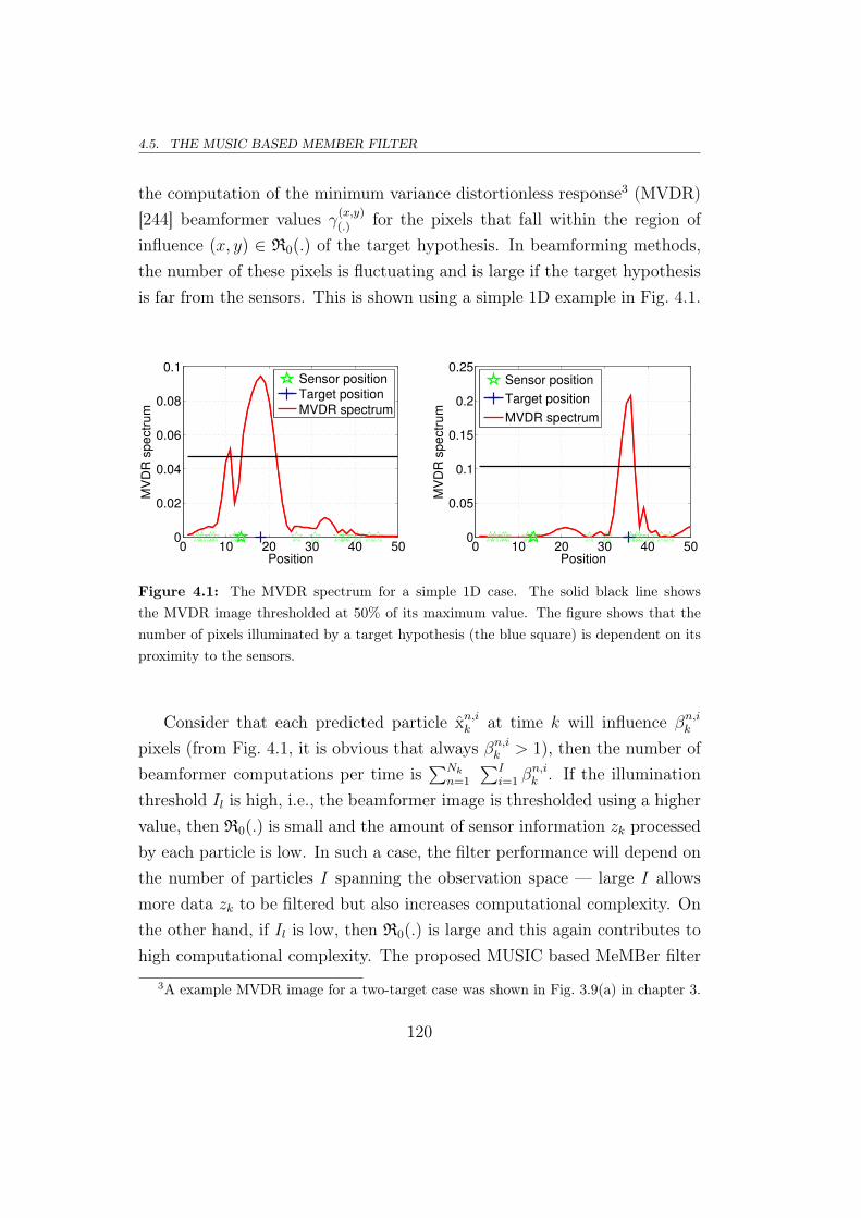
4.5. THE MUSIC BASED MEMBER FILTER
the computation of the minimum variance distortionless response3 (MVDR)[244] beamformer values γ(x,y)
(.) for the pixels that fall within the region ofinfluence (x, y) ∈ R0(.) of the target hypothesis. In beamforming methods,the number of these pixels is fluctuating and is large if the target hypothesisis far from the sensors. This is shown using a simple 1D example in Fig. 4.1.
0 10 20 30 40 500
0.02
0.04
0.06
0.08
0.1
Position
MV
DR
sp
ectr
um
Sensor position
Target position
MVDR spectrum
0 10 20 30 40 500
0.05
0.1
0.15
0.2
0.25
Position
MV
DR
sp
ectr
um
Sensor position
Target position
MVDR spectrum
Figure 4.1: The MVDR spectrum for a simple 1D case. The solid black line showsthe MVDR image thresholded at 50% of its maximum value. The figure shows that thenumber of pixels illuminated by a target hypothesis (the blue square) is dependent on itsproximity to the sensors.
Consider that each predicted particle xn,ik at time k will influence βn,ikpixels (from Fig. 4.1, it is obvious that always βn,ik > 1), then the number ofbeamformer computations per time is
∑Nkn=1
∑Ii=1 β
n,ik . If the illumination
threshold Il is high, i.e., the beamformer image is thresholded using a highervalue, then R0(.) is small and the amount of sensor information zk processedby each particle is low. In such a case, the filter performance will depend onthe number of particles I spanning the observation space — large I allowsmore data zk to be filtered but also increases computational complexity. Onthe other hand, if Il is low, then R0(.) is large and this again contributes tohigh computational complexity. The proposed MUSIC based MeMBer filter
3A example MVDR image for a two-target case was shown in Fig. 3.9(a) in chapter 3.
120

CHAPTER 4. THE MUSIC BASED MEMBER FILTER
requires the computation of only INk MUSIC values every time step. Thisfeature makes the filter computationally superior to the MeMBer filter forbeamformer images. In this work, for implementating the “MeMBer filterfor beamformer images,” the complete image γ(.) is first constructed usingMVDR beamforming and then thresholded using the illumination thresholdIl to obtain that part of the image γ(x,y)
(.) that is influenced by the targethypothesis. γ(x,y)
(.) is then fed into (4.11) to compute the likelihood.
4.6 Simulation results
All the simulations presented here consider tracking acoustic sources in a 2Denvironment which includes three echo paths with 1 second reverberationtime for 60 dB decay. The targets are constrained to move with position 0mto xmaxm in a line located 10m from another parallel line containing the 5
sensors whose positions are chosen from U [0, xmax]. The state of the targetis xk = (x, vx)
T where x is the position and vx is the velocity. ()T denotesmatrix transpose. The time evolution of xk is described as
xk =
1 T
0 1
xk−1 + qk−1 (4.15)
where the duration between two observations is T = 1s and the additiveprocess noise qk−1 ∼ N (0, Q) where the uncorrelated covariance matrix is
Q =
3 0
0 0.5
(4.16)
The sensor signals are obtained using the model described in (4.1). Thesensor noise vector is vk ∼ CN (0, R) where R is a diagonal with a varianceof σ2 = 0.1 corresponding to each sensor.
121

4.6. SIMULATION RESULTS
Demonstration
The proposed MUSIC based particle-MeMBer filter for tracking single/multiple,appearing/disappearing and crossing targets is demonstrated in Fig. 4.2. Itcan be seen that the filter quickly locks on and tracks the targets with highaccuracy. If a target disappears, the existence probability of the BernoulliRFS becomes low, thereby eliminating the track. The use of the Markovtransition prior as the proposal distribution is known to be sub-optimal andthe performance of the proposed scheme could be enhanced using an im-
10 20 30 40 50
10
20
30
40
50
60
70
80
90
100
Time [s]
Positio
n [m
]
Ground truth
Filter estimate
Figure 4.2: Filter estimates compared to the ground truth. The targets move along a1D grid of xmax = 100m width. The number of particles that approximate the pdf of eachelement in the multi-Bernoulli RFS is I = 1000. f = 4KHz and ν = 1500m/s. The SNR is30dB. The Poisson mean of the number of new-born targets is λB = 10. The probability oftarget survival (chosen to be constant) is pS = 0.8. The pruning threshold is Tprune = 0.6.The merging threshold is Tmerge = 1m. The filter runs for 50 time steps.
122

CHAPTER 4. THE MUSIC BASED MEMBER FILTER
proved importance distribution. Nevertheless, it can be seen that the trackinitialisation and deletion are conducted very effectively.
For the multi-target scenario described in Fig. 4.2, the MMSE-based-MDL estimate used to evaluate the noise eigenvectors Un used in (4.14) isshown in Fig. 4.3 and it can be observed that the technique provides an ac-curate estimate of the actual number of targets (even at low SNR levels).
10 20 30 40 500
1
2
3
4
5
6
Time [s]
No. of ta
rgets
SNR=30dB
SNR=6dB
Actual
Figure 4.3: The MMSE-based-MDL estimate of the number of targets, versus time.
Demonstration of target resolving ability
Secondly, the ability of the proposed MUSIC based particle-MeMBer filterto effectively resolve close targets is demonstrated. For this, the scenario
123

4.6. SIMULATION RESULTS
described in Fig. 4.4 is used. Here, two targets cross each other twice. Thismotion is realistic for real-world scenarios where targets often move in ap-proximately straight lines with constant velocity and occasionally make anabrupt manoeuvre [222].
10 20 30 40 50
10
20
30
40
50
60
Time [s]
Positio
n [m
]
Target 1
Target 2
Figure 4.4: The ground truth of the two targets used to obtain the evaluation results inFig. 4.5, Fig. 4.6, Fig. 4.7, Fig. 4.9, Fig. 4.10 and Fig. 4.14. The target positions coincideexactly at k = 13 and at k = 38.
In view of the fact that the PHD and the MeMBer filters cannot operatedirectly on sensor array data, for comparison with the proposed method, theacoustic signals are first converted into the minimum variance distortionlessresponse (MVDR) beamformer image which is the observation for the MeM-Ber filter. For the PHD filter, the image is further thresholded to generatethe finite set point measurement feed. The proposed MUSIC based MeMBer
124

CHAPTER 4. THE MUSIC BASED MEMBER FILTER
filter, however, operates on the acoustic signals. The super resolution prop-erty of MUSIC aids in resolving close targets and keeping the tracks separatefor a longer duration.
Fig. 4.5, Fig. 4.6 and Fig. 4.7 show the particle evolution (for the groundtruth in Fig. 4.4) for the proposed MUSIC based MeMBer, the MeMBer forimage and the PHD filters respectively. It can be observed that the proposedfilter resolves close targets better than the others. Before the first crossingat k = 13, it can be seen that while the PHD and the MeMBer filters keep
10 20 30 40 50
10
20
30
40
50
60
Time [s]
Positio
n [m
]
Figure 4.5: Evolution of the particles with time in the proposed MUSIC based particle-MeMBer filter. The targets move along a one dimensional grid grid of xmax = 60m width.The number of particles for each target state hypothesis is I = 1000. f = 4KHz andν = 1500m/s. The SNR is 30dB. For simplicity, it is assumed that the number of targetsis known; hence λB = 0. The survival probability is pS = 0.8. The pruning threshold isTprune = 0.6. The merging threshold is Tmerge = 1m. The filter runs for 50 time steps.
125

4.6. SIMULATION RESULTS
the targets separate only until the 6th and 9th time samples respectively, theproposed filter keeps the targets separate until the 11th time step. After thesecond crossing at k = 38, the PHD and MeMBer filters resolve the targetsonly after k = 46 and k = 44 respectively, and the proposed MeMBer filterseparates the targets from the 40th time sample.
10 20 30 40 50
10
20
30
40
50
60
Time [s]
Positio
n [m
]
Figure 4.6: Evolution of the particles with time in the particle-MeMBer filter (for imagedata) [49, 196]. The system specifications described in the caption of Fig. 4.5 apply to thisfigure also. The illumination threshold Il is chosen to be 0 so that the entire image is fedto the filter.
126

CHAPTER 4. THE MUSIC BASED MEMBER FILTER
10 20 30 40 50
10
20
30
40
50
60
Time [s]
Positio
n [m
]
Figure 4.7: Evolution of the particles with time in the particle-PHD filter [272]. Thesystem specifications described in the caption of Fig. 4.5 apply to this figure also. Thedetection probability is pD = 0.95. Target birth is not considered. To obtain the pointtarget measurement feed, the beamformer image is thresholded at 70% of the maximumpeak. 1000 particles are used. To obtain state estimates, the k-means clustering approachof [169] is used.
To further illustrate the filters’ target resolving ability, the normalisedPHD function (evaluated over the entire 60m grid) for the proposed MUSICbased MeMBer, MeMBer and PHD filters is shown in Fig. 4.8. This PHDcorresponds to the ground truth in Fig. 4.4 at the 11th time step. For theMeMBer filter, the PHD function is evaluated from (2.103) in section 2.7.1 ofchapter 2. It can be observed that the proposed method successfully resolvesthe two targets while the other filters merge them inextricably (as is alsoseen in Fig. 4.5, Fig. 4.6 and Fig. 4.7).
127

4.6. SIMULATION RESULTS
0 10 20 30 40 50 600
0.1
0.2
0.3
0.4
0.5
0.6
Position [m]
PH
D f
un
ctio
n
MUSIC MeMBerMeMBer: I
l=0
PHD filter
Figure 4.8: Normalised PHD function of the MUSIC based MeMBer, MeMBer and PHDfilters at the 11th time step.
Evaluation of track accuracy
Thirdly, the accuracy of the filters (using the ground truth shown in Fig. 4.4)is tested. Fig. 4.9 shows the root mean square error (RMSE) for varying SNRlevels. It can be observed that that the proposed technique is very accurate.Its performance advantage as against the PHD and the MeMBer filters canbe attributed to the direct use of acoustic signals. At low SNR, spuriouspeaks in the beamformer image degrade the MeMBer filter performance.Moreover, its error increases with increasing Il. The unwanted peaks atlow SNR, in turn, increase the false alarms in the PHD filter observationset and adversely effects its performance. The joint filter operates usingthe true likelihood function in (4.2) with the number of targets fixed at
128
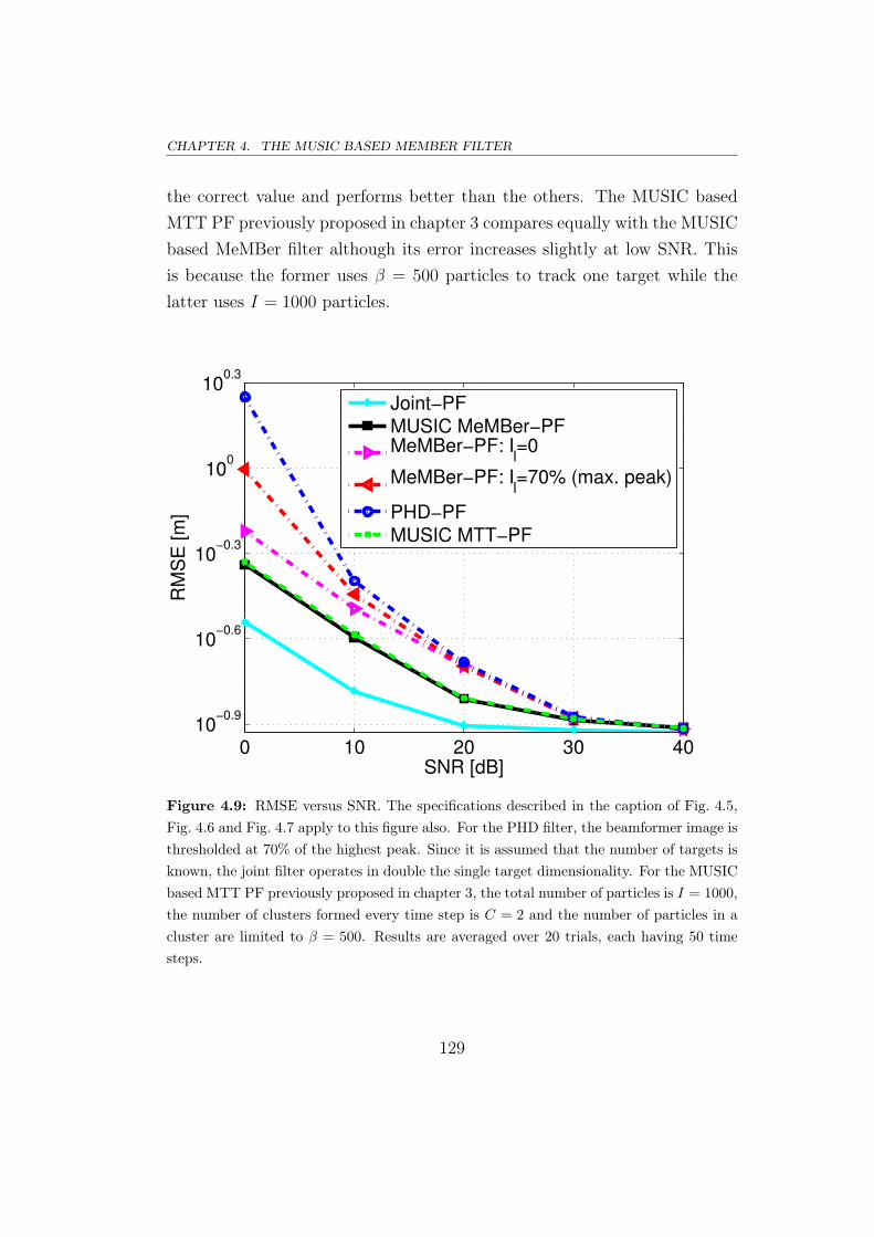
CHAPTER 4. THE MUSIC BASED MEMBER FILTER
the correct value and performs better than the others. The MUSIC basedMTT PF previously proposed in chapter 3 compares equally with the MUSICbased MeMBer filter although its error increases slightly at low SNR. Thisis because the former uses β = 500 particles to track one target while thelatter uses I = 1000 particles.
0 10 20 30 4010
−0.9
10−0.6
10−0.3
100
100.3
SNR [dB]
RM
SE
[m
]
Joint−PF
MUSIC MeMBer−PFMeMBer−PF: I
l=0
MeMBer−PF: Il=70% (max. peak)
PHD−PF
MUSIC MTT−PF
Figure 4.9: RMSE versus SNR. The specifications described in the caption of Fig. 4.5,Fig. 4.6 and Fig. 4.7 apply to this figure also. For the PHD filter, the beamformer image isthresholded at 70% of the highest peak. Since it is assumed that the number of targets isknown, the joint filter operates in double the single target dimensionality. For the MUSICbased MTT PF previously proposed in chapter 3, the total number of particles is I = 1000,the number of clusters formed every time step is C = 2 and the number of particles in acluster are limited to β = 500. Results are averaged over 20 trials, each having 50 timesteps.
129

4.6. SIMULATION RESULTS
Evaluation of computational complexity
Fourthly, the complexity of the filters (using the ground truth in Fig. 4.4)is shown in Fig. 4.10 by measuring the computational time to evaluate onecomplete time step for varying numbers of particles. It can be observed thatthe proposed filter requires fewer computational resources than the MeMBerfilter operating on the image data. This is because the MeMBer filter needs toconstruct 2I images, each having 60 pixels for the evaluation of (4.11) whilethe proposed technique requires only 2I MUSIC values. In the particle-PHDfilter, the majority of the time is consumed while evaluating the beamformerimage and hence the filter will be slower than the others when I / xmax. Inthis simulation, xmax = 60m is width of the surveillance region. The MUSIC
102
103
10−2
100
102
No. of particles (I)
Filt
er
co
mp
uta
tio
na
l tim
e [
s]
Joint filter
MUSIC MeMBer filterMeMBer filter: I
l=0
MeMBer filter: Il=70% (max. peak)
PHD filter
Figure 4.10: Time consumption for one time step versus I. The specifications describedin the caption of Fig. 4.9 apply to this figure also.
130

CHAPTER 4. THE MUSIC BASED MEMBER FILTER
based MTT PF exhibits low complexity requirements because it uses only Iparticles (in the dimensionality of a single target) to track the two targetswhile the proposed MUSIC based MeMBer filter uses 2I particles. The jointfilter uses I particles of double the dimension, and its complexity becomesunfavourable for larger numbers of targets. This can be observed in Fig. 4.11.The figure shows the computational time taken to evaluate the true likelihoodin (4.2) (used in the joint filter) and the MUSIC pseudo-likelihood in (4.14)(used in the proposed MUSIC based MeMBer filter) for 1000 particles whilevarying the number of targets. It can be observed that the true likelihoodcomputation quickly becomes resource expensive. The high computationalcomplexity of the proposed filter for the two target case in Fig. 4.10 can beattributed to merging and pruning operations. However, it can be seen from
0 2 4 6 8 100
0.2
0.4
0.6
0.8
1
1.2
1.4
No. of targets
Lik
elih
oo
d c
om
pu
tatio
na
l tim
e [
s]
True Likelihood
MUSIC pseudo−likelihood
MUSIC pseudo−likelihood + Prune + Merge
Figure 4.11: The computational time consumed in computing the likelihoods. Thenumber of particles used is 500. The results are averaged over 10000 trials.
131

4.6. SIMULATION RESULTS
Fig. 4.11 that the computation cost of pruning and merging operation doesnot rise like the likelihood for the joint filter (here the number of new-borntargets is NB ∼ Pois(λB) with λB = 18).
4.6.1 Evaluation of MUSIC based MTT filters
Finally, the MUSIC based MTT filtering methods proposed in this thesis —the MUSIC based MTT filter of chapter 3 and the MUSIC based MeMBerfilter of this chapter — are further analysed and tested. Firstly the effects ofusing MUSIC as a pseudo-likelihood are studied, and then the track accuracyof the methods for changing numbers of targets and harder target movementsis evaluated.
Numerical analysis on MUSIC pseudo-likelihood
Given that the MUSIC based MTT PF of chapter 3 and the MUSIC basedMeMBer filter of this chapter both use MUSIC as the pseudo-likelihood ofa particle, it is valid to investigate the faithfulness of MUSIC in accuratelyrepresenting the true likelihood. Fig. 4.12 shows the true likelihood and theMUSIC pseudo-likelihood evaluated over the entire 60m grid in the presenceof a single target. It can be observed that the MUSIC pseudo-spectrum hasa much narrower peak at the target location than that of the true likelihoodfunction, and hence will provide a good estimate of the target location but apoor estimate of the location uncertainty. This is further shown by the corre-sponding cumulative distribution functions (CDFs) in Fig. 4.13. The narrowpeak in MUSIC pseudo-spectrum causes its CDF to be truncated near thetails of the CDF of the true likelihood. This is shown using double arrows.
In a PF context, the narrow peaky nature of MUSIC will result in manyreplications of large weight particles during the resampling step, i.e., theparticle cloud could be too constrained. This can be overcome using a aux-iliary [135] PF approach or by introducing a few Markov chain Monte Carlo(MCMC) steps after resampling [127]. These approaches will increase the di-
132

CHAPTER 4. THE MUSIC BASED MEMBER FILTER
0 10 20 30 40 50 600
0.01
0.02
0.03
0.04
0.05
0.06
0.07
x−position [m]
Lik
elih
ood
True likelihood
MUSIC pseudo−likelihood
Ground truth location
Figure 4.12: The true likelihood and MUSIC pseudo-likelihood spectrums. The targetis exactly at 22m.
versity among particles. Nevertheless, the particle cloud can easily follow tar-gets if the process covariance Q is chosen such that its norm ||Q|| =
∑i,j Q
2i,j
is large.
If a single target scenario is considered with no target appearance or dis-appearance, the MUSIC based MTT PF of chapter 3 and the MUSIC basedMeMBer filter of this chapter are simply single target PFs, except that theweight of a particle is now the MUSIC pseudo value. Now, the faithfulness ofthe MUSIC pseudo-likelihood based single target PF is numerically tested interms of its conformity with the true-likelihood based single target PF. Forthis numerical testing, the well known Kolmogorov-Smirnov (KS) statistic[62] is used. The KS test has the advantage of providing a reliable measure
133

4.6. SIMULATION RESULTS
10 20 30 40 50 600
0.2
0.4
0.6
0.8
1
x−position [m]
cdf
True likelihood cdf
MUSIC likelihood cdf
Figure 4.13: CDFs for the normalised results in Fig. 4.12. The locations of maximumdeviation are shown with the arrows.
of the accuracy of the estimate of the posterior. The classical one-sample KStest evaluates the misfit between the CDFs of two univariate ordered datasets[273] by computing the largest absolute difference. For the KS testing inmulti-dimensional models [274], the two-sample KS test [275, 276] operatesby comparing the CDFs from two multi-dimensional datasets which are or-dered in some fashion. One method (as used here) is to compare the CDFsof the two samples with all combinations of sorting, and take the largest ofthe set of resulting KS statistics. KS testing for multi-dimensional data hasbeen used previously for other PF problems [277]. For the Markovian processmodel described in this section, and considering one target from the groundtruth shown in Fig. 4.4, Fig. 4.14 shows the two-sample KS statistic misfitof the MUSIC pseudo-likelihood based PF with the PF that operates using
134

CHAPTER 4. THE MUSIC BASED MEMBER FILTER
the true likelihood equation in (4.2). The KS values for the PF in whichthe likelihood is the MVDR value is also shown. Since the MUSIC andMVDR functions are not identical to a true likelihood, there is considerabledisagreement in the two filter representations. Although the disagreementdecreases with increasing I, it can be observed that the statistic begins toexhibit asymptotic behaviour from I u 500.
0 200 400 600 800 10000
0.1
0.2
0.3
0.4
0.5
0.6
0.7
No. of particles (I)
KS
sta
tistic
MUSIC
MVDR
Figure 4.14: The KS statistic disagreement [274] versus the number of particles. Theground truth shown in Fig. 4.4 is used, except that now only one target is considered. Thespecifications in the caption of Fig. 4.5 apply to this figure also. The results are averagedover 20 trials, each comprising 50 time steps.
Evaluation of track accuracy and target number estimation
Here, the track accuracy of the MUSIC based MTT filters is evaluated forchanging numbers of targets, i.e., target appearance and disappearance, and
135

4.6. SIMULATION RESULTS
for harder target movements. For this study, the 2D state model usedin section 3.7 of chapter 3 is employed. The target state is defined asxk = (x, y, vx, vy)
T where x, y are the positions and vx, vy are the veloci-ties along the x, y-axis. xk evolves with time in accordance to a Markovmodel in which the position is updated using a constant velocity model andthe velocity is updated using a random walk. The process noise is zero-meanGaussian distributed with uncorrelated covariance matrix having a varianceof 0.5 along each dimension. The specifications are as follows: (i) the surveil-lance region is a 4×4 2D space which includes a one second reverberation timefor 60 dB decay, (ii) a linear array of 5 sensors, located at an offset of 10malong the third dimension from the grid of target movement, is used, i.e., thesensor positions are x = 1, y = {1, 2, 3, 4, 5} and z = 10, (iii) the frequencyof operation is f = 4 kHz, (iv) the propagation velocity is ν = 1500m/s, and(v) the total number of time steps is 50.
In this testing, two MTT scenarios are used. The ground truth usedfor the first scenario is shown in Fig. 4.15 (and also in Fig. 4.16). The ac-tual target paths are plotted as solid lines in different colors. In this MTTscenario, two targets — the ones depicted using green and black solid lines— travel close to one another with nearly opposite velocities during timesk = 34, 35, 36. Three targets — the ones depicted using red, cyan and bluesolid lines — travel very close to one another approximately during timesk = 35, ..., 42. The targets represented in blue and red make a suddenmanoeuvre nearly at time k = 45. The ground truth used for the secondscenario is shown in Fig. 4.17 (and also in Fig. 4.18). The target paths areagain plotted as solid lines in different colors. In this MTT scenario, twotargets — the ones depicted using red and black solid lines — travel closeto one another approximately during times k = 19, ..., 22. Three targets —the ones depicted using blue, red, and cyan solid lines — travel close to oneanother approximately during times k = 26, ..., 32. Two targets — the onesdepicted using green and black solid lines — travel close to one another ap-proximately during times k = 35, 36. The targets represented in red and
136

CHAPTER 4. THE MUSIC BASED MEMBER FILTER
blue travel with opposite velocities when travelling close to each other. Thetarget represented in black makes a u-turn during times k = 29, ..., 35. Inboth the examples, it is ensured that two targets are not at the same posi-tion at the same time. The target starting position is indicated by a circleand the time of the target appearance is noted next to the circle. The finalposition of the target before its disappearance is indicated by a star and thetime step at which the target reaches this position is noted next to the star.Additionally, Fig. 4.15 and Fig. 4.17 demonstrate the operation of the MU-SIC based MTT PF of chapter 3 while Fig. 4.16 and Fig. 4.18 demonstratethe operation of the MUSIC based MeMBer filter of this chapter. The fil-
1 2 3 4 51
1.5
2
2.5
3
3.5
4
4.5
5
x−position [m]
y−
po
sitio
n [
m]
1 11
2126
2650
40
40
50
45
Figure 4.15: The first MTT scenario and the evolution of particles in the MUSIC basedMTT PF of chapter 3. The SNR is 27dB. In the filter, the number of particles I = 5000,the number of clusters is C = 8, the number of particles per cluster is regulated to β = 500,and the cluster looseness threshold to initiate and remove tracks is exp(−Tc) = 0.75.
137

4.6. SIMULATION RESULTS
1 2 3 4 51
1.5
2
2.5
3
3.5
4
4.5
5
x−position [m]
y−
po
sitio
n [
m]
1 11
2126
2650
40
40
50
45
Figure 4.16: The first MTT scenario and the evolution of particles in the MUSIC basedMeMBer filter of this chapter. The SNR is 27dB. In the filter, the survival probabilityis pS = 0.95, the number of new-born targets is NB ∼ Pois(λB) with λB = 10, the totalnumber of particles per Bernoulli set is I = 1000, the pruning threshold is Tprune = 0.65,and the merging threshold is Tmerge = 1m.
ters are demonstrated by showing the evolution of particles. These particlesare plotted as grey circles. While demonstrating the MUSIC based MTTPF, the figures shows only those particle clusters whose cluster looseness isexp(−Tc) ≥ 0.75. To overcome the problem of a too constrained particlecloud due to the narrow peaky nature of MUSIC, 7 MCMC transitions areintroduced [127] for each cluster after the regulation step. This slightly in-creases the diversity of the particles. It can be seen from the figures thatthe MUSIC based MTT filters (i) accurately track the targets, (ii) quicklydetect new-born targets, and (iii) successfully release lock of disappearing
138

CHAPTER 4. THE MUSIC BASED MEMBER FILTER
targets. It can also be observed that the track continuity is successfullymaintained by weighting the velocity component to be (in this example,three times) higher than the position component. Simulation videos demon-strating the filters’ implementation for both the MTT scenarios are availableat http://ecs.victoria.ac.nz/Groups/CSP/PublicationExtras.
1 2 3 4 51
1.5
2
2.5
3
3.5
4
4.5
5
x−position [m]
y−
po
sitio
n [
m]
1
16
11 6
31
5045
40
45
45
Figure 4.17: The second MTT scenario and the evolution of particles in the MUSIC basedMTT PF. The SNR is 27dB. The filter specifications listed in the caption of Fig. 4.15 applyto this figure also.
The track accuracy of various MTT filters for the first MTT scenariogiven in Fig. 4.15 (and Fig. 4.16) and the second MTT scenario given inFig. 4.17 (and Fig. 4.18) is shown in Fig. 4.19 and Fig. 4.20 respectively.The figures show the RMSE of the MUSIC based MTT filters proposed inthis thesis and other state-of-the-art Bayes’ MTT filters, for varying SNR
139

4.6. SIMULATION RESULTS
1 2 3 4 51
1.5
2
2.5
3
3.5
4
4.5
5
x−position [m]
y−
po
sitio
n [
m]
1
16
11 6
31
5045
40
45
45
Figure 4.18: The second MTT scenario and the evolution of particles in the MUSICbased MeMBer filter. The SNR is 27dB. The filter specifications listed in the caption ofFig. 4.16 apply to this figure also.
levels. Error bars that represent a 90% confidence interval are also shown.It can be observed that the results are consistent with those in Fig. 3.11 andFig. 4.9. Except for the joint filter, no other filter assumes knowledge aboutthe actual number of targets. The joint filter provides a best possible targetstate estimate when the actual number of targets is known and hence can beused as a reference for analysing the performance of the other MTT methods.In the other filters, the error is computed from the time the filter detects atarget. In the RFS filters — the PHD and the MeMBer filters — the MVDRbeamformer image is evaluated over the observation space with a resolutionof 0.1m. From both the figures, it can be observed that joint filter exhibitsthe superior performance. The performance of the RFS filters drops heavily
140

CHAPTER 4. THE MUSIC BASED MEMBER FILTER
5 10 15 20 25 30 35 4010
−0.7
10−0.5
10−0.3
10−0.1
SNR [dB]
Po
sitio
n e
rro
r [m
]
Joint filter
PHD filter
MeMBer (Image) filter
MUSIC MeMBer filter (Ch. 4)
MUSIC MTT PF (Ch. 3)
Figure 4.19: RMSE versus SNR for the first MTT scenario. The results are averagedover 100 trials, each having 50 time steps. The filter specifications are as follows. The jointfilter operates on I = 1000 particles with dimensionality equal to the number of targets.The PHD filter: (i) the detection and survival probabilities are pD = 0.9 and pD = 0.95
respectively, (ii) the number of new-born targets is NB ∼ Pois(λB) with λB = 10, (iii) thePoisson mean of the number of false alarms is λF = 10, (iv) the point target detectionsare obtained by thresholding the beamformer image at 70% of its maximum peak, (v)the total number of particles is I = 1000, and (vi) the state estimates are obtained usingthe k-means clustering approach of [169]. For the MeMBer filter for image data: (i) thesurvival probability is pS = 0.95, (ii) the number of new-born targets is NB ∼ Pois(λB)
with λB = 10, (iii) the beamformer image is thresholded at 70% of its maximum peakwhile computing the likelihood ratio, (iv) the total number of particles per Bernoulli setis I = 1000, (v) the pruning threshold is Tprune = 0.65, and (vi) the merging thresholdis Tmerge = 1m. For the MUSIC based MeMBer filter proposed in this chapter: thespecifications of the MeMBer filter for image data apply to this filter also, except thatbeamforming is not required. For the MUSIC based MTT PF of chapter 3: (i) the totalnumber of particles is I = 5000, (ii) the number of clusters is C = 8, (iii) the maximumnumber of particles in a cluster is β = 500, and (iv) the cluster looseness threshold toinitiate and remove tracks is exp(−Tc) = 0.75.
141
4.6. SIMULATION RESULTS
with decreasing SNR: in the PHD filter this is due to increased number offalse alarms and missed detections caused by the thresholding process, andin the MeMBer filter this is due to the spurious peaks in the image. Due tothe avoidance of thresholding, the MeMBer filter exhibits better performancethan the PHD filter. It can be seen that both the MUSIC based MTT filtersdisplay better performance than the RFS filters and give results close to thatof the joint filter. This is due to a more direct use of the array data by virtueof using MUSIC. The reduced track accuracy of the MUSIC based MTT PFas compared to that of the MUSIC based MeMBer filter could be attributedto the reduced number of particles assigned to a target — the MUSIC basedMeMBer filter uses 1000 particles per target while the MUSIC based MTTPF uses only 500 particles per target.
5 10 15 20 25 30 35 4010
−0.7
10−0.5
10−0.3
10−0.1
SNR [dB]
Po
sitio
n e
rro
r [m
]
Joint filter
PHD filter
MeMBer (Image) filter
MUSIC MeMBer filter (Ch. 4)
MUSIC MTT PF (Ch. 3)
Figure 4.20: RMSE versus SNR for the second MTT scenario. The details mentionedin the caption of Fig. 4.19 apply to this figure also.
142

CHAPTER 4. THE MUSIC BASED MEMBER FILTER
Now the ability of the MUSIC based MTT PF of chapter 3 to accuratelyestimate the number of targets is evaluated. Figs. 4.21 and 4.22 show theMUSIC based MTT PF estimate of the number of targets versus time, for thefirst and second MTT scenarios shown in Figs. 4.15 and 4.17 respectively. Thetarget number estimate is computed by finding the number of clusters thatdeclare target presence, i.e., the number of clusters whose exp(−Tc) ≥ 0.75.The additional MCMC transitions are not considered in this test. It can beseen that the filter provides an accurate estimate of the number of targetseven at low SNR. A possible reason for the over-estimation of the targetnumber at low SNR when multiple targets travel in close proximity could be
10 20 30 40 500
1
2
3
4
5
6
7
8
Time [s]
Nu
mb
er
of
targ
ets
Actual
MUSIC MTT PF (SNR = 6dB)
MUSIC MTT PF (SNR = 36dB)
Figure 4.21: The MUSIC based MTT PF estimate of the number of targets, versus time,for the first MTT scenario. The results are averaged over 100 trials, each having 50 timesteps. The filter specifications described in the caption of Fig. 4.15 apply to this figurealso.
143

4.7. CONCLUSION AND SUMMARY
due to (i) the over-estimation by the MMSE based MDL method, or (ii) afree cluster near multiple tight clusters being influenced by the resamplingprocess to declare target presence. Nevertheless, it can be observed that theproblem does not persist in time as clustering and regulation are conductedat every time step.
10 20 30 40 500
1
2
3
4
5
6
7
8
Time [s]
Nu
mb
er
of
targ
ets
Actual
MUSIC MTT PF (SNR = 6dB)
MUSIC MTT PF (SNR = 36dB)
Figure 4.22: The MUSIC based MTT PF estimate of the number of targets, versus time,for the second MTT scenario. The results are averaged over 100 trials, each having 50
time steps. The filter specifications described in the caption of Fig. 4.15 apply to thisfigure also.
4.7 Conclusion and summary
This chapter addressed the problem of Bayesian RFS filtering for phasedsensor array observation models. State-of-the-art RFS filters — the PHD
144
CHAPTER 4. THE MUSIC BASED MEMBER FILTER
and the MeMBer filters, in spite of overcoming the high computational com-plexity of the theoretically accurate joint filter, do not possess a suitableframework to operate directly on the phased array data and instead operateon images derived from the data. Converting the phased array data causessubstantial information and resolution loss.
This chapter proposed a MUSIC based MeMBer filter, the key innova-tion of which is to use for the likelihood in the “MeMBer filter for imageobservations,” the MUSIC pseudo-spectrum — a function which has as itsdomain the state space of a single target. The advantages of the developedfilter are; a) a more direct use of the array data resulting in improved trackaccuracy at low SNR, b) low computational complexity by replacing the like-lihood ratio with the MUSIC value, and c) effective resolution of close targetsby the super-resolution property of the MUSIC. The validity and merits ofthe proposed method were demonstrated using simulations. Referring backto section 1.3.1 of chapter 1, it can be stated that the research goal 2 thataims to overcome problem 2 has been successfully achieved by the proposedMUSIC based MeMBer filter.
145

4.7. CONCLUSION AND SUMMARY
146
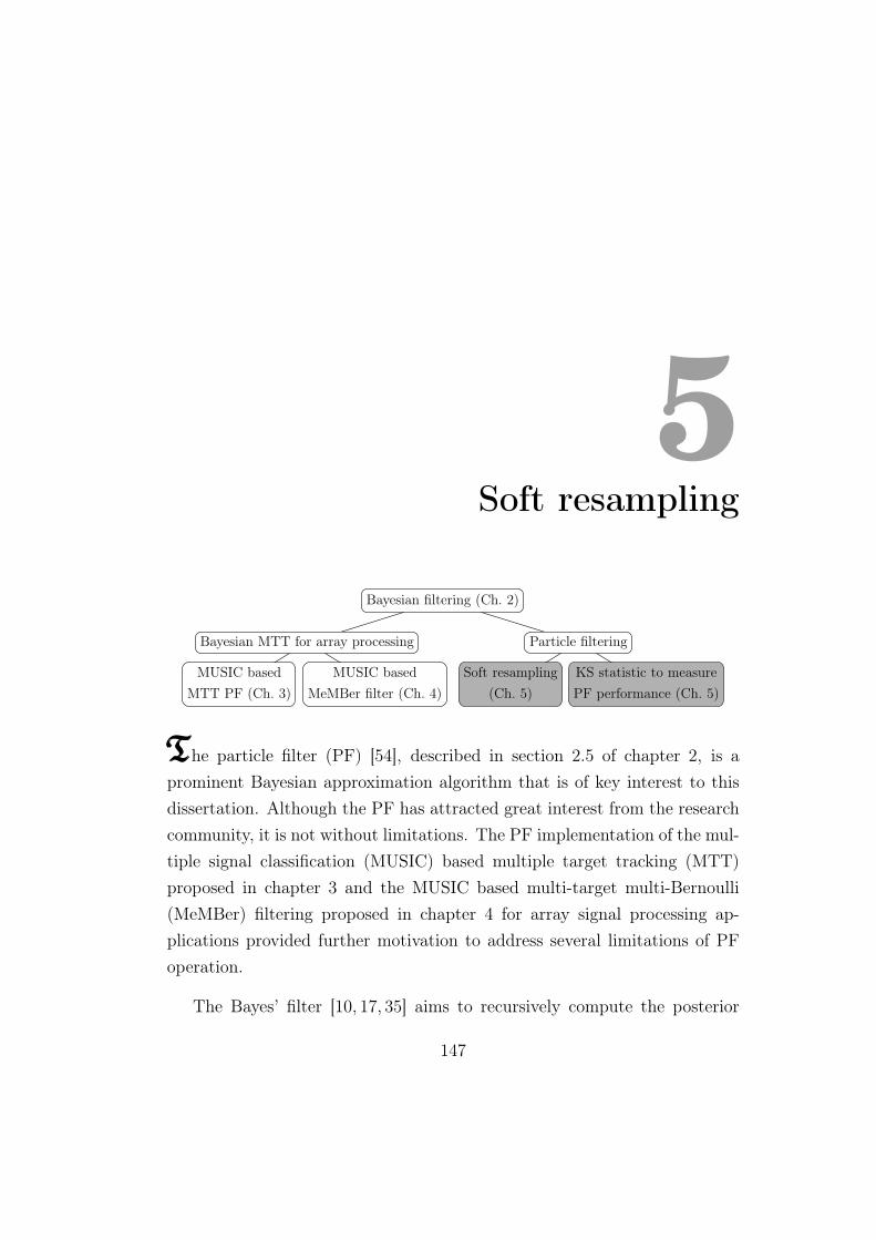
5Soft resampling
Bayesian filtering (Ch. 2)
Bayesian MTT for array processing
MUSIC basedMTT PF (Ch. 3)
MUSIC basedMeMBer filter (Ch. 4)
Particle filtering
Soft resampling(Ch. 5)
KS statistic to measurePF performance (Ch. 5)
TTThe particle filter (PF) [54], described in section 2.5 of chapter 2, is aprominent Bayesian approximation algorithm that is of key interest to thisdissertation. Although the PF has attracted great interest from the researchcommunity, it is not without limitations. The PF implementation of the mul-tiple signal classification (MUSIC) based multiple target tracking (MTT)proposed in chapter 3 and the MUSIC based multi-target multi-Bernoulli(MeMBer) filtering proposed in chapter 4 for array signal processing ap-plications provided further motivation to address several limitations of PFoperation.
The Bayes’ filter [10, 17, 35] aims to recursively compute the posterior
147

probability distribution function (pdf) of the state of the target(s) [44]. How-ever, it is known that Bayes’ filtering is intractable [56] due to high dimen-sional integration and this intractability is overcome using approximate so-lutions [32]. The PF [21] approximates the Bayes’ posterior pdf by a setof weighted independent point target representations, which in this contextare called particles. Particle filtering involves an intermediary resamplingstep [118–121] in which particles with lower weights are replaced by copiesof those with large weights. The major drawback in PF resampling, as iden-tified in problem 3 of section 1.3.2 in chapter 1, is that the process resultsin loss of the information contained in those particles having low weightsand consequently the effectiveness of the PF is affected if these low weightscontain potential target information. The research goal 3 in section 1.3.2of chapter 1 — to develop a resampling scheme that preserves more of theinformation contained in low weight particles and ensure that the accuracyof the posterior approximation of the developed resampler is not affected —aims to overcome this drawback. This chapter presents the development ofthis novel resampling approach and illustrates how the goal is achieved.
The resampling step in the PF involves rejection and replacement of par-ticles based on their weights. This causes major adjustments to the informa-tion contained in the final particle set representation. Hence, as identified inproblem 4 of section 1.3.2 in chapter 1, a numerical measure of the resamplerperformance is required. The research goal 4 in section 1.3.2 of chapter 1that deals with this requirement aims to propose a quantifiable measure forassessing the faithfulness of the PF in accurately representing the posterior.A numerical test that achieves this goal is presented and used in this chapter.
The chapter is organised as follows: The related work in state-of-the-artresamplers with regard to information retention is outlined in section 5.1.After stating the problem in section 5.2, the proposed resampling methodand its modification are presented in section 5.3 and section 5.4 respectively.
148
CHAPTER 5. SOFT RESAMPLING
In section 5.5, the numerical test for assessing the resampler performance isdescribed. The evaluation results are presented in section 5.6 and concludingremarks are given in section 5.7.
5.1 Related work
The PF [110], described in sections 2.5.3 and 2.5.4 of chapter 2, can be re-garded as a technique that uses two fundemental approaches in succession.The first, sequential importance sampling (SIS), specifies the process of draw-ing new particles at each time step based on a state equation [52, 127, 135]and updating their weights. The weight of a particle gives a probabilisticmeasure of the correctness of a hypothesis (particle). By itself, SIS resultsin a large variance of the weights and this ultimately results in one particlehaving all the weight — an inefficiency known as degeneracy. This degen-eracy is overcome using a second stage, resampling, that replaces the lowerweight particles by those with larger weights [119, 120].
The focus of this chapter is in PF resampling. Resampling techniquescan be classified broadly into; a) stochastic, and b) deterministic. A fewpopular state-of-the-art resampling strategies are outlined in section 2.5.4 ofchapter 2. The stochastic resamplers, namely the multinomial [241], strat-ified [242], systematic [52, 136] and residual [53] resamplers, duplicate theparticles in proportion to their weights. This could result in the dismissalof moderate/low weight particles along with their weights. That is to say,stochastic resampling could result in loss of the information contained in apotential low weight particle — a particle that is gradually gaining weighteither because the target is making a turn towards it or it is in the processof declaring a covert target. This problem is more evident in residual resam-pling because the method always discards the low weight particles (refer toits operation in section 2.5.4 of chapter 2). Moreover, the stochastic resam-plers reset all the weights to the same number. The implication that everyresampled particle is equally valid in representing the posterior pdf of the
149

5.1. RELATED WORK
target state is only asymptotically true. Deterministic resampling schemes[120, 122], on the other hand, are threshold-based. Partial resampling [120]proposes to keep the set of moderately weighted particles unchanged and re-sample the set of dominant and negligible particles. However, the reweightingis now based on the size of the sets but not on the individual weights. Thiscauses loss of potential information contained in the negligible particles.
The detection of very covert targets using a PF relies on the accumula-tion of information over many consecutive observations, i.e., a covert targetshould be tracked for some time before declaring its presence. The contem-porary resampling procedures discussed above impede this accumulation. Inscenarios where particles are searching for new (very covert) targets, state-of-the-art resamplers quickly create fairly tight clusters so that there are notenough particles to span the entire observation space by the time a targetappears, that is to say, the standard PF operating on state-of-the-art resam-plers believes hastily: a characteristic that is unsuitable for the detectionof covert targets. Hence the contemporary resamplers can be termed “hardresamplers.” To overcome this lack of information retention in a standardPF, the track-before-detect (TBD) PF [55, 56, 133], described section 2.5.7of chapter 2, has been proposed. The target state birth and death modellingin the TBD PF aids in information retention. When the target is absent,most particles in the TBD PF are non-existent (dead) and take the maximumweight, i.e., if the existence parameter of the ith particle is Ei
k = 0, then itsweight is wik = 1. Hence using any contemporary resampler will result inmany replications of these non-existent particles. The few existing particleswhose Ei
k = 1 (the proportion of particles whose Eik = 1 is defined in the
transitional probability matrix) remain in a loose cloud. When the targetappears and start manoeuvring, the dead particles gradually come into exis-tence and their weights will now be their likelihood of representing the truetarget, i.e., if Ei
k = 1, then wik will be the weight update equation. That isto say, the higher the likelihood of the particle xik in hypothesising the targetcorrectly, the longer its existence parameter Ei
k = 1 and hence the stronger
150
CHAPTER 5. SOFT RESAMPLING
the belief that xik is tracking a target. The ability of the TBD PF in detect-ing new targets is dependent on the total number of particles I; using fewerparticles results in an insufficient number of particles to span the observationspace for new targets, but using more particles increases computational load.
5.2 Motivation
It is noteworthy that when the number of particles I is large, the poste-rior distribution represented by the PF using any state-of-the-art resamplerdiscussed above will be an accurate representation of the true distribution[116, 117, 222]. However it is usually the case that I is limited. The firstobjective in this chapter is to develop a “soft resampling” scheme that; a)aids in improved information accumulation over time, b) preserves the in-formation contained in low weight particles, and c) thereby enhances theposterior representation with fewer particles. The motivating idea to achievethis objective is to reduce the variance between the original and the re-sampled weights by the process of proportional redistribution (also termedreplication) and reweighting of particles, i.e., the particles are replicated inproportion to their weights, and the weights are reweighted in proportion tothe number of replications. The aim is to achieve this without affecting theaccuracy in representing the true posterior.
The second objective in this chapter is to propose a numerically cal-culable measure to assess the PF approximation performance and test thefaithfulness of the proposed resampler in accurately representing the poste-rior. The motivating idea to achieve this objective is to use the well-knownKolmogorov-Smirnov (KS) statistic [273] which is a standard test to com-pare distributions. Using the Kalman filter [20] as a reference, the KS misfitbetween the optimal Kalman filter distribution and the PF representationcould be computed.
151

5.3. SOFT RESAMPLING
5.3 Soft resampling
In this section, the soft resampling algorithm [61] is proposed. The conven-tional resamplers replicate the particles in proportion to their weights, i.e.,the number of replications of a particle xik will be1 nik = bIwikc. Then thetotal number of replications is K =
∑Ii=1 n
ik and generally K < I. Hence
the information contained in the I−K low weight particles whose nik = 0 fori = K + 1, ..., I, and their weights, does not appear in the resampled particleset. Losing this information could be problematic if the target is covert or ismaking a sharp manoeuvre towards a low weight particle.
Soft resampling addresses this problem. The key idea is to reduce thevariance between the actual and the resampled particle weights, i.e., for un-biased resampling, we want
E
[ ∑∀j, 1≤j≤I : x∗jk =xik
w∗jk
]= wik (5.1)
where {xik, wik}Ii=1 and {x∗jk , w∗jk }Ij=1 respectively is the weighted particle set
before and after resampling. The method to achieve (5.1) is as follows: Afterthe prediction and weight update steps, all the I weights are normalised andsorted in descending order. Then for each index i = 1, ..., I, the number ofreplications of the ith particle xik is given by
Γxik= max{1, bIwikc} (5.2)
This indicates that a particle whose bIwikc ≥ 1 will be replicated accordingto its weight (i.e., a multinomial selection) and a particle whose bIwikc < 1
will appear once (i.e., retention of low weight particles). Based on this rule,the new resampled particles with indices j = `, ..., `+ Γxik
− 1 are
xjk = xik (5.3)1This multinomial selection of the number of replications of a particle has been dis-
cussed in section 2.5.4 of chapter 2.
152
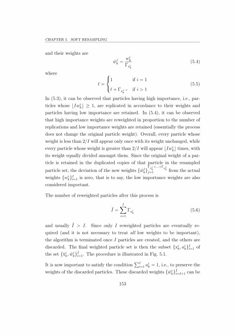
CHAPTER 5. SOFT RESAMPLING
and their weights are
wjk =wikΓxik
(5.4)
where
` =
1 if i = 1
`+ Γxi−1k
if i > 1(5.5)
In (5.3), it can be observed that particles having high importance, i.e., par-ticles whose bIwikc ≥ 1, are replicated in accordance to their weights andparticles having low importance are retained. In (5.4), it can be observedthat high importance weights are reweighted in proportion to the number ofreplications and low importance weights are retained (essentially the processdoes not change the original particle weight). Overall, every particle whoseweight is less than 2/I will appear only once with its weight unchanged, whileevery particle whose weight is greater than 2/I will appear bIwikc times, withits weight equally divided amongst them. Since the original weight of a par-ticle is retained in the duplicated copies of that particle in the resampled
particle set, the deviation of the new weights {wjk}Γ
x1k
+...+ΓxIk
j=1 from the actualweights {wik}Ii=1 is zero, that is to say, the low importance weights are alsoconsidered important.
The number of reweighted particles after this process is
I =I∑i=1
Γxik(5.6)
and usually I > I. Since only I reweighted particles are eventually re-quired (and it is not necessary to treat all low weights to be important),the algorithm is terminated once I particles are created, and the others arediscarded. The final weighted particle set is then the subset {xik, aik}Ii=1 ofthe set {xik, wik}Ii=1. The procedure is illustrated in Fig. 5.1.
It is now important to satisfy the condition∑I
i=1 aik = 1, i.e., to preserve the
weights of the discarded particles. These discarded weights {wik}Ii=I+1 can be
153

5.3. SOFT RESAMPLING
1 2 3 4 5 6 7 8
1/I
2/I
3/I
w1
3
w2
2w3
w4
w5w6
w7w8
Discard
Figure 5.1: Illustration of soft resampling. The figure shows weights of 8 particles; theweight vector w = [0.3529, 0.2995, 0.1604, 0.0749, 0.0428, 0.0321, 0.0267, 0.0107]. Amongthe 8 particles, the first particle has a weight of 3.3/I and hence gets 3 copies each weightedat w1
3 = 1.1I . The second particle has a weight of 2.8/I and hence gets 2 copies each
weighted at w2
2 = 1.4I . The other particles’ weights are left unchanged since they are
all less than 2/I. The last 3 particles are discarded since only 8 particles are eventuallyrequired.
reallocated to the retained weights {aik}Ii=1 in one of the two following ways;
Renormalisation: The retained weights are renormalised as
bik =aik∑Ii=1 a
ik
(5.7)
such that the total weight of the discarded particles is shared among all theremaining weights.
154

CHAPTER 5. SOFT RESAMPLING
Redistribution: The total discarded weight is
aspare = 1−I∑i=1
aik (5.8)
This weight is redistributed (or shared) only among the lower weight particlesas follows: find the particle index y such that
aspare + aIk + aI−1k + ...+ aI−yk ≤ aI−y−1
k (5.9)
Then the new weights are
bik =
aik for i = 1, ..., y − 1
aspare+∑Is=y a
sk
yfor i = y, ..., I
(5.10)
This method further reduces the weight variance because it allocates thediscarded weight only to low importance weights and does not modify thehigh importance weights.
The soft resampling presented in this section was found to introduce a biasin (5.1). This motivates the work of the next section.
5.4 Soft systematic resampling
In this section, a modification to the previously presented soft resampler isproposed. The rationale behind this proposal is discussed in section 5.4.1and the algorithm is then presented in section 5.4.2.
5.4.1 Motivation for soft systematic resampling
Retaining the information contained in the particles with low weights is cru-cial in the detection of very covert targets [55] and in the tracking of highlymanoeuvring targets, especially when the number of particles is limited. Softresampling [61] proposed in the previous section aids in this retention. In
155

5.4. SOFT SYSTEMATIC RESAMPLING
soft resampling, the particles having weights greater than 2/I are replicatedusing (5.3) and their weights are revised using (5.4). Once the particle limitI is reached, the redundant particles and their weights are discarded. Theinformation contained in these weights is retained by renormalisation or re-distribution. However the redundant particles — particles located near thetails of the cumulative distribution function (cdf) of the posterior density,i.e., the low weights particles that lie near the boundary of the particle set— are discarded all the time. This perpetual elimination causes a bias in(5.1). Discarding these particles could prove detrimental especially when theweights of the particles close to the target are very large, e.g., the MUSICbased MTT PF in chapter 3 or [256]. These large weight particles are repli-cated more times causing many lower weight particles that lie near the edgesof the particle set to be eliminated. As a result, the PF approximation istruncated near the tails of the cdf thereby leading to an inaccurate posteriorpdf. This problem is less evident in the stochastic resamplers because theyresample all the particles with non-zero probability thus ensuring that notevery low weight particle is lost perpetually.
The soft systematic resampling approach [278] presented in this sectionis an extension and correction to the soft resampling technique and presentsa scheme to overcome the problem of discarding the low weight particles allthe time. The main idea is to first use a modified variant of soft resamplingwithout discarding any particles and then stochastically resample the lowerweights using the systematic resampler [52, 136]. Hence, the technique istermed soft systematic resampling.
5.4.2 Soft systematic resampling algorithm
To overcome the problem of perpetually discarding low weight particles insoft resampling, this thesis proposes to resample a few lower weight particleswith non-zero probability. This can be done by using a systematic resampler[52]. The systematic resampler is used to stochastically resample a few lower
156

CHAPTER 5. SOFT RESAMPLING
weight particles so that not every low weight particle is eliminated all thetime. The consequential soft systematic resampling [278] in presented here.
After the SIS step, the weights are normalised and sorted in descendingorder. For a particle xik, if its weight wik > 2/I, xik is replicated
Γxik= max{1, bαIwikc} (5.11)
times, where 0 < α ≤ 1. Low values for α correspond to less replicationsof the larger weights. α can be used to regulate the spread of the largeweights, particularly when the likelihood of the particle closest to the targetis very large. Based on this principle the new resampled-reweighted particleset {xik, wik}Ii=1 is obtained using (5.3) and (5.4), where I is specified in (5.6).Note that the combined weight of the resampled particles for a particularindex i is the same before and after resampling, and is independent of α.
Then Nlow lower weight particles are stochastically resampled. Here,
Nlow = min
{I , bβ(I − I)e
}(5.12)
The term β ≥ 1 regulates the value of Nlow such that a large β resultsin more low weight particles being stochastically resampled. The weightedparticle set {xik, wik}Ii=I−Nlow+1
is then fed to the systematic resampler afternormalising its weights. Since only I particles are eventually required, thenumber of particles the resampler generates is limited to
Nresamp = Nlow − (I − I) (5.13)
These Nresamp particles will then replace the particles {xik}Ii=I−Nlow+1. This
process ensures that not all the I − I particles (these are the low weightparticles that lie near the edge of the particle cloud) are eliminated all thetime. The resampled particles are then reweighted as
wik =
∑Ij=I−Nlow+1 w
jk
Nresamp, i = I −Nlow + 1, ..., I (5.14)
157

5.4. SOFT SYSTEMATIC RESAMPLING
The remaining I−I weighted particles are then discarded. The final weightedparticle set is then the subset {xik, aik}Ii=1 of the set {xik, wik}Ii=1. The softsystematic resampling is illustrated in Fig. 5.2.
1 2 3 4 5 6 7 8
1/I
2/I
3/I
w1
3
w2
2w3
w4
w5w6
w7w8
Nlow
Nresamp
Discard
Figure 5.2: Illustration of soft systematic resampling with α = 1 and β = 2, for thesame weight vector given in the caption of Fig. 5.1. The original sample size is I = 8.The replication and reweighting process generates I = 11 particles. From (5.12), thenumber of low weights particles to be stochastically resampled is Nlow = 6, i.e., particleswith indices i = I − Nlow + 1, ..., I = 6, ..., 11, are stochastically resampled to generategenerate Nresamp = 3 particles. These Nresamp particles will replace particles with indicesi = I−Nlow+1, ..., I = 6, ..., 8. The weights of particles with indices i = I−Nlow+1, ..., I =
6, ..., 8, are modified using (5.14). Finally, the last I − I = 3 weighted particles arediscarded.
158

CHAPTER 5. SOFT RESAMPLING
5.4.3 Analysis of properties of the soft resampler
Here, the unbiased property of soft (systematic) resampling is analysed us-ing a simple example. As defined in (5.1), the soft resampler is said to beunbiased if the weight of a particle before resampling is completely preservedin each of its duplicated copies, i.e., if
wik − E
[ ∑∀j, 1≤j≤I : x∗jk =xik
w∗jk
]= 0 (5.15)
where {xik, wik}Ii=1 and {x∗jk , w∗jk }Ij=1 respectively is the weighted particle set
before and after resampling. Fig. 5.3 shows the bias analysis for a set of 100
samples having uniformly random weights. These (sorted) weights are shownin Fig. 5.3(a). Figs. 5.3(b) and (d) show the error between the weight of aparticle before resampling and the expected value of the total weight in eachof the duplicated copies of that particle, i.e., the computation
wik − E
[ ∑∀j, 1≤j≤I : x∗jk =xik
w∗jk
]
Fig. 5.3(c) shows the variance of the total weight contained in all the dupli-cated copies of a particle, i.e., the computation
Var
[ ∑∀j, 1≤j≤I : x∗jk =xik
w∗jk
]
It can be observed from the figure that the weight error and weight vari-ance in the soft resamplers is much smaller when compared to that of theconventional stochastic resamplers. This is because the former preserve thecomplete weight of a particle in each of its duplicated copies. Also note thedifference in the order of magnitude of the weight error and weight variancefor the soft and stochastic resamplers. The low weight error in soft (system-atic) resampling indicates that the actual weight of a particle is retained inthe new particle set. This leads to improved information retention over time.
159

5.4. SOFT SYSTEMATIC RESAMPLING
0 50 1000
0.005
0.01
0.015
0.02
Sample Number
We
igh
t
(a) Actual weight.
20 40 60 80 100−1
0
1x 10
−4
Sample Number
We
igh
t E
rro
r
(b) Weight error.
20 40 60 80 1000
1
2
3
4
5x 10
−5
Sample Number
We
igh
t V
aria
nce
Soft
Soft systematic: (α,β)=(0.95,1.5)
Systematic
Multinomial
(c) Weight variance.
0 20 40 60 80 100−4
−2
0
2
4x 10
−15
Sample Number
We
igh
t E
rro
r
Soft
Soft systematic: (α,β)=(0.95,1.5)
(d) Weight error.
Figure 5.3: Soft resampler bias analysis. The number of particles (samples) is I = 100.The results are computed over 1000 realisations. The legend of (c) applies to (b) also. Thesoft and soft systematic resamplers are plotted separately in (d) for better visualisation.
Since the weights are uniform, the number of duplications of a particle is zero(in this example). Hence the soft resampler does not suffer from bias. Thebias analysis when only a few particles have large weights is shown in Fig. 5.4.In this example, the (sorted) weights of 100 samples are shown in Fig. 5.4(a).It can be observed from Fig. 5.4(b) that the soft resampler suffers a bias,albeit having a very low weight error and variance. This is because the lowweights that lie near the tail of the distribution are completely discarded.This bias is successfully overcome in the soft systematic resampler by virtue
160

CHAPTER 5. SOFT RESAMPLING
of stochastically resampling a few low weight particles. It can be noted thatas β increases, the performance of the soft systematic resampler approachesthat of the systematic resampler.
0 20 40 60 80 1000
0.02
0.04
0.06
0.08
0.1
Sample Number
We
igh
t
(a) Actual weight.
20 40 60 80 100−1
0
1x 10
−4
Sample NumberW
eig
ht
Err
or
(b) Weight error.
20 40 60 80 1000
1
2
3
4
5x 10
−5
Sample Number
We
igh
t V
aria
nce
Soft
Soft systematic: (α,β)=(0.95,1.5)
Systematic
Multinomial
(c) Weight variance.
20 40 60 80 100−2
−1
0
1
2x 10
−5
Sample Number
We
igh
t E
rro
r
Soft
Soft systematic: (α,β)=(0.95,1.5)
(d) Weight error.
Figure 5.4: Soft resampler bias analysis. The number of particles (samples) is I = 100.The results are computed over 1000 realisations. The legend of (c) applies to (b) also. Thesoft and soft systematic resamplers are plotted separately in (d) for better visualisation.
5.5 The numerical measure of PF performance
Here, a quantitative measure to evaluate the accuracy of the PF in repre-senting the posterior is introduced. The numerical test presented here can
161

5.5. THE NUMERICAL MEASURE OF PF PERFORMANCE
be used in a generic PF framework.
It is known that for linear Gaussian models, the Kalman filter [20], de-scribed in section 2.4 of chapter 2, provides a optimal tracking estimate[32, 81, 90]. This thesis proposes to test the faithfulness of the PF in accor-dance to its KS statistic agreement [62] with the theoretically optimal Kalmanfilter. The KS test2 has the advantage of providing a reliable measure of theaccuracy [279] of the estimate of the posterior. However, the test has beenunder-utilised in the PF literature and has never been used to measure re-sampler performance. The classical one-sample KS test evaluates the misfitbetween the cdfs of two uni-dimensional ordered datasets [273] by comput-ing the largest absolute difference. If the empirical distribution Xn for a setof I independent and identical distributed (i.i.d) uni-dimensional particles{xi}Ii=1 is defined as
Xn(y) =number of elements in the sample ≤ y
I=|{xi : xi ≤ y}|
I(5.16)
Then the KS statistic for a given cdf X is
κKS = supy |Xn(y)−X(y)| (5.17)
This procedure however, cannot be applied to multi-dimensional distributionsbecause there is no unique way to order the data. KS testing for multi-dimensional Gaussian models [274] can be conducted using the two-sampleKS statistic [275, 276] by comparing the cdfs from two multi-dimensionaldatasets which are ordered in some fashion. One method is to comparethe cdfs of the two samples with all possible combinations of sorting, andtake the largest of the set of resulting KS statistics. Multi-dimensional KStesting has been used previously for other PF problems [277, 280]. A fewother performance evaluation schemes that may also be adaptable to PFperformance metrics can be found in [281].
In this thesis, for KS testing in linear Gaussian and multi-dimensional2The KS test was first used in this dissertation in chapter 4.
162

CHAPTER 5. SOFT RESAMPLING
models, a modified KS testing approach is proposed. The rationale for thisproposal is to exploit the availability of the mean and covariance estimateprovided by the theoretically optimal Kalman filter. The procedure will nowbe presented.
5.5.1 The modified KS testing approach
Mathematically, the proposed KS statistic testing is conducted as follows:At time k, let the Kalman mean estimate be µk and the covariance estimatebe Pk. Let Gk be the Cholesky decomposition of Pk. Consider that theD-dimensional resampled particle set {xik, wik}Ii=1 is available and that theparticle states along the dth dimension are denoted by {xid,k}Ii=1. Firstly,each dimension of the particle state as represented by the particles are de-meaned and de-correlated using the theoretically optimal Kalman mean andcovariance. This is done according to
yid,k = G−1k (xid,k − µk) (5.18)
for i = 1, ..., I and d = 1, ..., D. The new particles {yid,k}i=1,...,I, d=1,...,D arethen sorted as
{Ψid,k, θ
id,k}Ii=1 = sort({yid,k}Ii=1) ; d = 1, ..., D (5.19)
where {Ψid,k}Ii=1 contains the sorted particle states along the dth dimension
and {θid,k}Ii=1 contains the indices of the particle states (in the dth dimension)in the sorted order. Then for i = 1, ..., I and d = 1, ..., D, the cdf of theparticle states is evaluated according to
ck(d, i) =i∑
j=1
wθjd,kk (5.20)
The emperical cdf is the error function related to the integral of the standardnormal distribution and is measured according to
ck(d, i) = Φ(Ψid,k) =
1 + erf(Ψid,k/√
2)
2(5.21)
163

5.5. THE NUMERICAL MEASURE OF PF PERFORMANCE
where the error function is described as
erf(s) =2√π
∫ s
0
exp(−t2) dt (5.22)
Finally, the KS statistic is measured by conducting the one-sample KS testalong each dimension separately and then taking the maximum KS deviationvalue amongst all the dimensions. That is,
κKS = supd supi |ck(d, i)− ck(d, i)| (5.23)
In words, the procedure is as follows: After resampling, the particle states arede-meaned and de-correlated using the theoretically optimal Kalman meanand covariance. Then the particle states along each dimension are sorted andthe cdf (along that dimension) is constructed by evaluating the cumulativesum of the weights taken in the sorted order. Finally, the one-sample KStest is conducted along each dimension separately by comparing the cdf ofthe particle states and the error function, and maximum KS deviation valueamongst all the dimensions is taken.
If the PF representation is identical to that of the Kalman filter distri-bution, then (5.18) will result in a set of uncorrelated particles which arenormally distributed with zero mean and unit variance. The cdf of the statesof these particles (after sorting) will be close to that of the error function, i.e.,the KS deviation will be small. Conversely, if the PF representation is notidentical to that of the Kalman filter distribution, then the cdf of the particlestates will differ from that of the error function, i.e., the KS deviation will belarge. Overall, the proposed method tests the representation misfit of the PFagainst a reference distribution — the theoretically optimal Kalman filter.The procedure is now illustrated using a simple example.
Illustration of the proposed KS test:Consider a two dimensional state space. Let the Kalman filter mean beµ = [6, 8]T and its covariance be
164

CHAPTER 5. SOFT RESAMPLING
P =
0.85 0.2
0.2 0.7
The first scenario is shown in Fig. 5.5. Here, 1000 particles are drawn froma 2D normal distribution with mean µPF = µ and covariance PPF = P .These particles are plotted (as red dots) over the contour describing theKalman filter distribution. The de-mean and de-correlation of these particleswill result in a new set of particles (plotted as black dots). The contourof a standard normal distribution is also shown for reference. Since thePF representation is identical to that of the Kalman filter distribution, thedeviation of the cdf of particles from the error function of N (0, 1) is small.
−5 0 5 10
−2
0
2
4
6
8
10
x−axis
y−
axis
Actual particles
Modified particles
(a) PF representation
−4 −2 0 2 40
0.5
1
1.5
Position [m]
CD
F
PF CDF − Dim 1Error function − Dim 1PF CDF − Dim 2Error function − Dim 2
(b) cdf
Figure 5.5: KS test illustration when the PF representation is close to the optimalKalman filter distribution.
The second scenario is shown in Fig. 5.6. Here, 100 particles are drawn froma 2D normal distribution with mean µPF = µ and covariance PPF = P . Sincethe PF representation is identical to that of the Kalman filter distribution,the deviation of the cdf of particles from the error function ofN (0, 1) is small.However, the figure shows that the accuracy of approximation depends onthe number of particles I, and insufficient I leads to poor representation ofthe distribution N (0, 1). Hence the deviation of the cdf of particle states
165

5.6. EVALUATION
from the error function of N (0, 1) is larger when compared to the case ofI = 1000.
−5 0 5 10
−2
0
2
4
6
8
10
x−axis
y−
axis
Actual particles
Modified particles
(a) PF representation
−4 −2 0 2 40
0.5
1
1.5
Position [m]C
DF
PF CDF − Dim 1Error function − Dim 1PF CDF − Dim 2Error function − Dim 2
(b) cdf
Figure 5.6: KS test illustration when the PF representation is close to the optimalKalman filter distribution, but the number of particles I is low.
The third scenario is shown in Fig. 5.7. Here, 1000 particles are drawn froma 2D normal distribution with mean and covariance different from µ andP respectively. Since the PF representation is not identical to that of theKalman filter distribution, the deviation of the cdf of particles from the errorfunction of N (0, 1) is large.
5.6 Evaluation
The validity and efficacy of the proposed soft and soft systematic resamplingmethods is demonstrated here. Although the primary interest of this thesis ison phased sensor arrays, other sensor models are used here in the context ofa) being able to test the KS performance of the resamplers, and b) availabilityof real image data. The proposed methods are first evaluated using imageobservations in section 5.6.1. Secondly, the methods are tested by comparingwith the optimal Kalman filter in section 5.6.2 using a 2D linear Gaussianmodel.
166

CHAPTER 5. SOFT RESAMPLING
−5 0 5 10
0
5
10
x−axis
y−
axis
Actual particles
Modified particles
(a) PF representation
−5 0 50
0.5
1
1.5
Position [m]
CD
F
PF CDF − Dim 1Error function − Dim 1PF CDF − Dim 2Error function − Dim 2
(b) cdf
Figure 5.7: KS test illustration when the PF representation is not identical to the optimalKalman filter distribution.
5.6.1 The proposal analysed using a TBD example
Here, the efficacy of the proposed methods is tested using a TBD applicationwith single target tracking using Gaussian image models. The model spec-ifications can be found in Ch. 11 of [56] and also in [55]. The state of thetarget is defined as xk = (x, vx, y, vy, B)T where x, y are the positions andvx, vy are the velocities along the x, y-axes. B is the intensity contribution ofthe target to the image. ()T denotes matrix transpose. The time evolutionof xk is described as
xk =
1 T 0 0 0
0 1 0 0 0
0 0 1 T 0
0 0 0 1 0
1 T 0 0 1
xk−1 + qk−1 (5.24)
167

5.6. EVALUATION
where the additive process noise qk−1 ∼ N (0, Q) with
Q =
0.0013
T 3 0.0012
T 2 0 0 0
0.0012
T 2 0.001 T 2 0 0 0
0 0 0.0013
T 3 0.0012
T 2 0
0 0 0.0012
T 2 0.001 T 2 0
0 0 0 0 0.01 T
(5.25)
The duration between two observations is T = 1s. The observations are20 × 20 staring camera snapshots. The snapshot intensity at the (n,m)thpixel at time k is
z(n,m)k =
N (γ(n,m)k (xk), σ
2) if the target is present
N (0, σ2) otherwise(5.26)
where the intensity contribution γ(n,m)k (xk) by a target with state xk =
(x, vx, y, vy, B)T to the (n,m)th pixel is
γ(n,m)k (xk) =
∆n∆mB
2πΣ2exp(− (n∆n − x)2 + (m∆m − y)2
2Σ2
)(5.27)
The blurring parameter is Σ = 0.7. (∆n,∆m) = (1, 1) is the center of the(n,m)th pixel. σ is the camera background noise standard deviation at eachpixel.
The test runs for 30 frames (time steps) as follows: (i) the target is absent inthe first 7 frames — the softness of the particles during this period is tested,(ii) the target appears in the 8th frame — the time to lock onto the targetstarting from the 8th frame is tested, and (iii) the target disappears fromthe 25th frame — the time to release target lock is tested. All the results areaveraged over 50 iterations.
Softness
Firstly, the softness of the proposed methods is tested during the first 7
frames without the presence of a target. Fig. 5.8 shows the softness (a.k.a
168

CHAPTER 5. SOFT RESAMPLING
looseness or variance) of 128 particles measured according to
Cloose =
∑||xik −
∑Ii=1
xikI||2
I(5.28)
for varying sensor noise standard deviation σ at each pixel in the snapshot.All the resamplers are tested on a standard PF (i.e., not on the TBD PFframework). It can be observed that by the 7th frame, the proposed soft andsoft systematic resamplers leave a more loosely-fitted cluster than that of theconventional resamplers. The renormalised and redistributed variants of softresampling exhibit almost similar performance. It can be seen that the softsystematic resampler with low α regulates the spread of the large weights, i.e.,
0.5 1 1.5 2 2.5 3 3.5 40
1
2
3
4
5
6
7
8
9
sensor noise standard deviation (σ) [m]
Lo
ose
ne
ss o
f th
e p
art
icle
s
Soft systematic: (α, β)= (0.95, 1)
Soft systematic: (α, β)= (0.95, 4)
Soft−renormalised
Soft−redistributed
Partial deterministic
Systematic
Residual
Stratified
Multinomial
Figure 5.8: Looseness of 128 particles versus pixel noise standard deviation. The particlesare propagated in a standard PF operating with the various resampling schemes shown inthe figure. For partial deterministic resampling [120], the thresholds to find the dominantand negligible particles are 1/I and 1/I2 respectively.
169

5.6. EVALUATION
low α generates fewer inter-particle replacements and this results in a morelooser cluster. It can also be observed that the particle cloud gets tighter withincreasing β and will approach the performance of the systematic resampler.Overall, the proposed resamplers leave a soft particle cluster and this featureaids in a faster lock (when compared to that of standard non-TBD PFs) whenthe target appears.
Time to lock
Secondly, the locking ability of the various filters is tested wherein the targetappears in the 8th frame and starts manoeuvring. Fig. 5.9 shows the numberof frames taken, beginning from the 8th frame, to lock the target. The pro-posed resamplers are tested on a standard PF. The conventional resamplersdo not effectively aid in successive accumulation of the information sufficientfor the detection of covert targets. This problem is overcome using the TBDPF. Hence the conventional resamplers are tested on both the standard PFand TBD PF frameworks. It can be observed in Fig. 5.9 that since the softresampler leaves a loose particle cluster at the 7th frame, there are enoughparticles in the vicinity of target appearance to detect and quickly lock ontothe target. The figure also indicates that the speed of lock in the soft sys-tematic resampler decreases with increase in β (due to high stochasticity inparticle replacements) and decrease in α (due to fewer particle replacements).It can also be observed that the traditional “hard” resamplers operating onthe standard PF take more frames to lock the target than that of the TBDPF counterpart (because in the TBD PF, target detection is aided by thetransition probability assigned to the particles). The stratified and residualresamplers exhibit almost similar performance to that of the systematic re-sampler and are hence not shown, both here in Fig. 5.9 and also in Fig. 5.10.
Time to release target lock
Thirdly, the time taken to release the target lock is tested: the target ap-peared at the 8th frame, manoeuvred until the 24th frame and then disap-
170
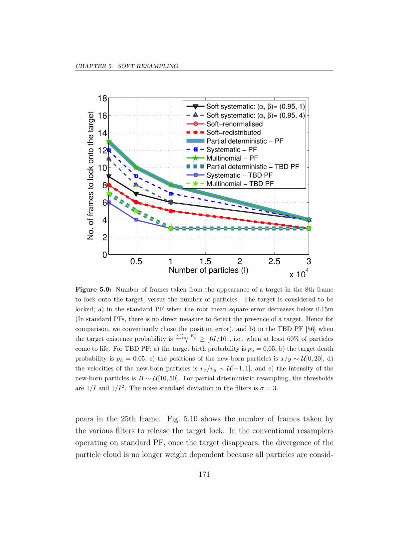
CHAPTER 5. SOFT RESAMPLING
0.5 1 1.5 2 2.5 3
x 104
0
2
4
6
8
10
12
14
16
18
Number of particles (I)
No
. o
f fr
am
es t
o lo
ck o
nto
th
e t
arg
et
Soft systematic: (α, β)= (0.95, 1)
Soft systematic: (α, β)= (0.95, 4)
Soft−renormalised
Soft−redistributed
Partial deterministic − PF
Systematic − PF
Multinomial − PF
Partial deterministic − TBD PF
Systematic − TBD PF
Multinomial − TBD PF
Figure 5.9: Number of frames taken from the appearance of a target in the 8th frameto lock onto the target, versus the number of particles. The target is considered to belocked; a) in the standard PF when the root mean square error decreases below 0.15m(In standard PFs, there is no direct measure to detect the presence of a target. Hence forcomparison, we conveniently chose the position error), and b) in the TBD PF [56] whenthe target existence probability is
∑Ii=1 Ei
k
I ≥ b6I/10e, i.e., when at least 60% of particlescome to life. For TBD PF; a) the target birth probability is pb = 0.05, b) the target deathprobability is pd = 0.05, c) the positions of the new-born particles is x/y ∼ U [0, 20], d)the velocities of the new-born particles is vx/vy ∼ U [−1, 1], and e) the intensity of thenew-born particles is B ∼ U [10, 50]. For partial deterministic resampling, the thresholdsare 1/I and 1/I2. The noise standard deviation in the filters is σ = 3.
pears in the 25th frame. Fig. 5.10 shows the number of frames taken bythe various filters to release the target lock. In the conventional resamplersoperating on standard PF, once the target disappears, the divergence of theparticle cloud is no longer weight dependent because all particles are consid-
171
5.6. EVALUATION
ered to be equally probable in representing the posterior. The divergence ofthe particles then depends on the process noise sequence qk−1, i.e., for highlyobservable targets, the matrix norm ||Q|| =
∑i,j Q
2i,j is smaller and hence the
particle cloud divergence is slower, and vice versa. That is to say, the releaseof the target in a standard PF operating on conventional resamplers is notdependent on the resampler. Hence for the conventional resamplers, onlytheir TBD PF implementations are shown in the figure. Fig. 5.10 indicatesthat the TBD PF (using any resampler) releases the lock immediately oncethe target disappears. Releasing the target lock as soon as the target disap-
0.5 1 1.5 2 2.5 3
x 104
0
2
4
6
8
Number of particles (I)
No
. o
f fr
am
es t
o r
ele
ase
ta
rge
t lo
ck
Soft systematic: (α, β)= (0.95, 1)
Soft systematic: (α, β)= (0.95, 4)
Soft−renormalised
Soft−redistributed
Partial deterministic − TBD PF
Systematic − TBD PF
Multinomial − TBD PF
Figure 5.10: Number of frames taken from the disappearance of a target to releasethe target lock. Target is considered to be released; a) in the proposed method whenCloose > −log(0.3), and b) in the TBD PF when the target existence probability is∑I
i=1 Eik
I < b6I/10e [56]. The TBD PF system and partial deterministic resampling thresh-old specifications described in the caption of Fig. 5.9 apply to this figure also.
172

CHAPTER 5. SOFT RESAMPLING
pears could be problematic in cases where the target momentarily shuts off,or is obstructed by non-target objects like buildings, etc. The proposed softresamplers preserve the lower weights, and hence the standard PF operatingon these resamplers waits for some time (anticipating target reappearance)before releasing the target lock. Note that these results are very sensitiveto the parameters used for each filter type, and so these results of TBD andnon-TBD are not directly comparable.
Accuracy
Fourthly, the accuracy of the proposed soft resampling methods is tested forthe image observation models. Fig. 5.11 shows the root mean square error
0.5 1 1.5 2 2.5 3 3.5 40
0.05
0.1
0.15
0.2
0.25
sensor noise standard deviation (σ) [m]
rmse
[m
]
Soft systematic: (α, β)= (0.95, 1)
Soft systematic: (α, β)= (0.95, 4)
Soft−renormalised
Soft−redistributed
Partial deterministic
Systematic
Residual
Stratified
Multinomial
Figure 5.11: rmse versus the noise standard deviation σ. The number of particles isI = 128. The target is present all the time. The partial deterministic resampling thresholdspecifications described in the caption of Fig. 5.8 apply to this figure also.
173
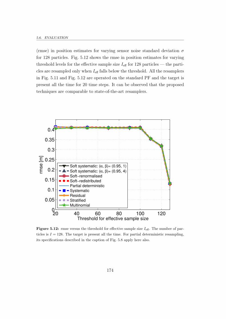
5.6. EVALUATION
(rmse) in position estimates for varying sensor noise standard deviation σ
for 128 particles. Fig. 5.12 shows the rmse in position estimates for varyingthreshold levels for the effective sample size Ieff for 128 particles — the parti-cles are resampled only when Ieff falls below the threshold. All the resamplersin Fig. 5.11 and Fig. 5.12 are operated on the standard PF and the target ispresent all the time for 20 time steps. It can be observed that the proposedtechniques are comparable to state-of-the-art resamplers.
20 40 60 80 100 1200
0.05
0.1
0.15
0.2
0.25
0.3
0.35
0.4
Threshold for effective sample size
rmse
[m
]
Soft systematic: (α, β)= (0.95, 1)
Soft systematic: (α, β)= (0.95, 4)
Soft−renormalised
Soft−redistributed
Partial deterministic
Systematic
Residual
Stratified
Multinomial
Figure 5.12: rmse versus the threshold for effective sample size Ieff. The number of par-ticles is I = 128. The target is present all the time. For partial deterministic resampling,its specifications described in the caption of Fig. 5.8 apply here also.
174

CHAPTER 5. SOFT RESAMPLING
5.6.2 The proposal compared with a Kalman filter
Here, the ability of the proposed soft and soft systematic resamplers to accu-rately represent the posterior and to retain more information is demonstrated.For this testing, a 2D linear Gaussian model is used so that comparison canbe made with the Kalman filter [20] which is known to give the optimal pos-terior. The target state is characterised by the position and velocity of thetarget as xk = (x, vx)
T . The process model is
xk =
[1 T
0 1
]xk−1 + qk−1 (5.29)
with T = 1s and the process noise qk−1 ∼ N (0, Q) where
Q =
0.95 0.2
0.2 0.75
The observation model
zk = xk + rk (5.30)
generates a clean though noisy point target measurement. The term “cleanmeasurement” implies there are no false alarms, clutter detections, missedobservations and/or out-of-sequence (OOS) observations3. The sensor noiseis rk ∼ N (0, R) with R = σ2I having the variance σ2 = 0.5 along eachdimension.
Accuracy of posterior representation
Fig. 5.13 shows the KS statistic of various filters for varying numbers ofparticles. It can be observed that the PF operating with the systematic re-sampler exhibits the best consensus with the theoretically optimal posteriorrepresentation obtained using the Kalman filter. It can also be observed that
3A OOS observation is a target detection at time k but received at a later time samplek + τ .
175
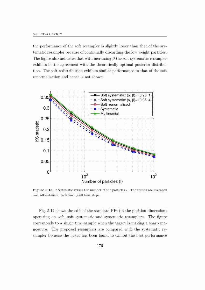
5.6. EVALUATION
the performance of the soft resampler is slightly lower than that of the sys-tematic resampler because of continually discarding the low weight particles.The figure also indicates that with increasing β the soft systematic resamplerexhibits better agreement with the theoretically optimal posterior distribu-tion. The soft redistribution exhibits similar performance to that of the softrenormalisation and hence is not shown.
102
103
0
0.05
0.1
0.15
0.2
0.25
0.3
0.35
Number of particles (I)
KS
sta
tistic
Soft systematic: (α, β)= (0.95, 1)
Soft systematic: (α, β)= (0.95, 4)
Soft−renormalised
Systematic
Multinomial
Figure 5.13: KS statistic versus the number of the particles I. The results are averagedover 50 instances, each having 50 time steps.
Fig. 5.14 shows the cdfs of the standard PFs (in the position dimension)operating on soft, soft systematic and systematic resamplers. The figurecorresponds to a single time sample when the target is making a sharp ma-noeuvre. The proposed resamplers are compared with the systematic re-sampler because the latter has been found to exhibit the best performance
176

CHAPTER 5. SOFT RESAMPLING
in terms of accurately representing the posterior in Fig. 5.13. In Fig. 5.14,the cdf in blue is obtained from (5.20) and the cdf in red is obtained from(5.21). It can be observed from the figure that while the soft resampler inFig. 5.14(d) does not properly treat the tails of the cdf because the methoddiscards the low weight particles all the time, the soft systematic resamplerin Fig. 5.14(b) overcomes this problem by stochastically resampling the par-ticles located near the tails of the cdf. For increasing β, the performance of
−5 0 50
0.2
0.4
0.6
0.8
1
PF cdfKalman cdf
(a) Soft systematic(α, β) = (0.95, 1)
−5 0 50
0.2
0.4
0.6
0.8
1
(b) Soft systematic(α, β) = (0.95, 4)
−5 0 50
0.2
0.4
0.6
0.8
1
(c) Systematic.
−5 0 50
0.2
0.4
0.6
0.8
1
(d) Soft.
Figure 5.14: cdfs for PFs operated using soft, soft systematic and systematic resamplers.These cdfs correspond to the position of a target. The legend of Fig. 5.14(a) applies toFig. 5.14(b,c,d) also.
177
5.6. EVALUATION
the proposed soft systematic resampler will approach that of the systematicresampler. Fig. 5.14(c) indicates that the systematic resampler based PF ap-proximation exhibits agreeable representation of the posterior described bythe theoretically optimal Kalman filter. The soft resampling (with renormal-isation) can be considered as soft systematic resampling with (α, β) = (1, 0).Therefore as observed in Fig. 5.14(a), decreasing the number of replicationsby reducing α will cause inaccuracies in posterior representation but the fea-ture can be used to address other PF problems, e.g., to increase the diversityof the particles when the weights of the particles near a target are very large[256].
Information retention
The proposed soft and soft systematic resamplers are analysed in terms oftheir ability to retain more information over successive time steps and therebyaid in a faster lock. For this test, the 2D linear Gaussian model described insection 5.6.2 is again used. Here, the particles are initialised with unit covari-ance and a mean that is 8m away from the actual target. This arrangementresults in a particle set that is just near the actual target by the time filteringstarts. This arrangement requires retention of the weight information overtime for a faster lock. Fig. 5.15 illustrates how fast the target is detected byshowing the drop in the rmse of the PF estimates for 10 time samples. Itcan be inferred that by appropriate reweighting and retaining more informa-tion contained in the lower weights, the soft and soft systematic resamplerslock onto the targets faster than the systematic resampler that regards allthe particles as equally weighted. The target in this test is allowed to makesharp manoeuvres, hence it is highly probable that the target could movetowards a low weight particle. By ensuring that not all low weight particlesare lost all the time, the soft systematic resampler aids in faster lock thanits soft counterpart. The soft redistributed variant exhibits almost similarperformance to that of soft renormalised variant and hence is not shown.
178

CHAPTER 5. SOFT RESAMPLING
2 4 6 8 100
2
4
6
8
10
12
Time [s]
rmse
[m
]
Soft systematic: (α, β)= (0.95, 4)
Soft−renormalised
Systematic
Kalman
Figure 5.15: rmse versus time samples. The number of particles I = 1024. The resultsare averaged over 100 instances, each having 10 time steps.
Accuracy
The accuracy of the various resamplers is tested for the same 2D linear Gaus-sian model. Fig. 5.16 shows the rmse in position for varying sensor noisevariance σ2 for 1024 particles. Again, the soft redistributed variant exhibitsalmost similar performance to that of the soft renormalised variant and hencenot shown. It can be observed that the proposed techniques are comparableto state-of-the-art resamplers.
179
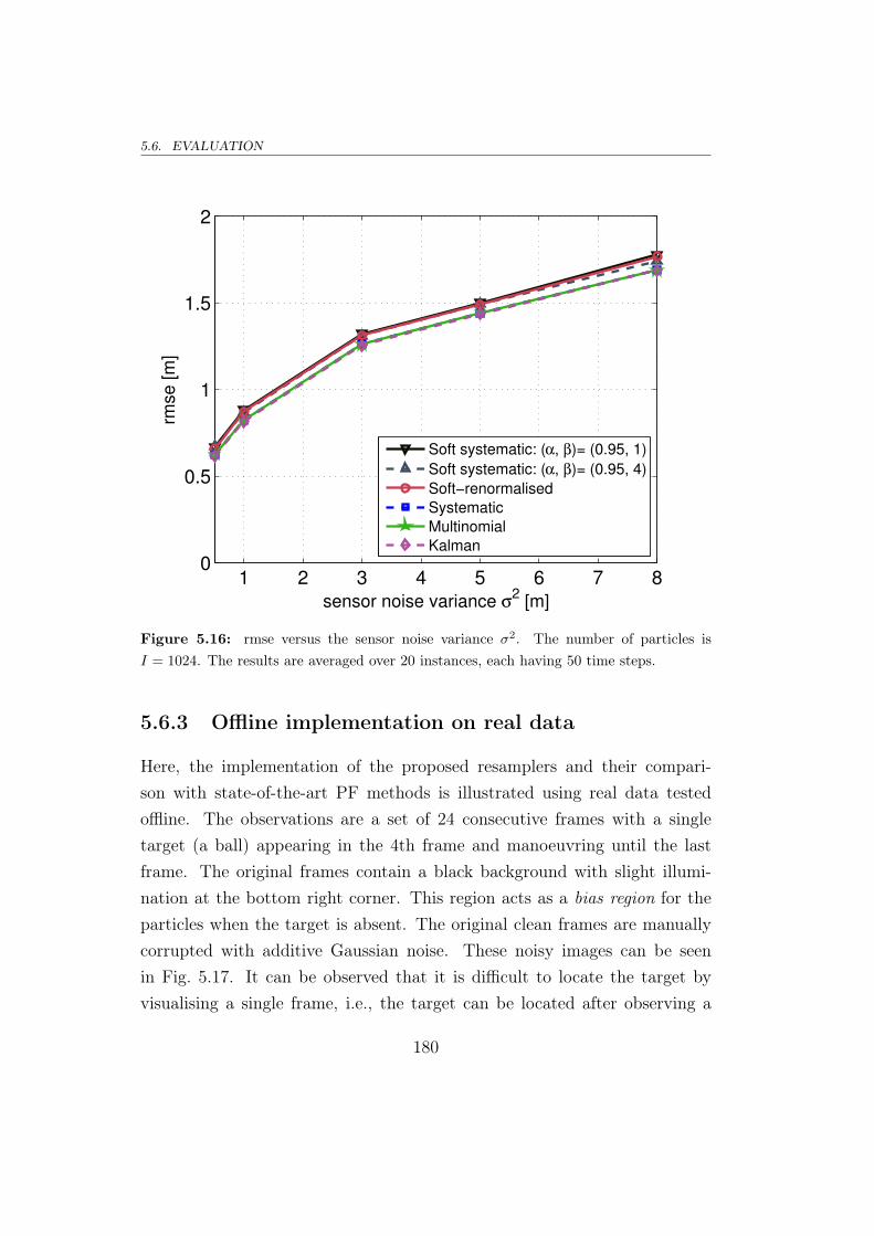
5.6. EVALUATION
1 2 3 4 5 6 7 80
0.5
1
1.5
2
sensor noise variance σ2 [m]
rmse
[m
]
Soft systematic: (α, β)= (0.95, 1)
Soft systematic: (α, β)= (0.95, 4)
Soft−renormalised
Systematic
Multinomial
Kalman
Figure 5.16: rmse versus the sensor noise variance σ2. The number of particles isI = 1024. The results are averaged over 20 instances, each having 50 time steps.
5.6.3 Offline implementation on real data
Here, the implementation of the proposed resamplers and their compari-son with state-of-the-art PF methods is illustrated using real data testedoffline. The observations are a set of 24 consecutive frames with a singletarget (a ball) appearing in the 4th frame and manoeuvring until the lastframe. The original frames contain a black background with slight illumi-nation at the bottom right corner. This region acts as a bias region for theparticles when the target is absent. The original clean frames are manuallycorrupted with additive Gaussian noise. These noisy images can be seenin Fig. 5.17. It can be observed that it is difficult to locate the target byvisualising a single frame, i.e., the target can be located after observing a
180

CHAPTER 5. SOFT RESAMPLING
few frames in succession — a replica of a covert target tracking problem.These noisy images are then fed to the PFs operating on 500 particles. Theevolution of the particles in these PFs is shown in Fig. 5.18 and Fig. 5.19.The particles are plotted on the ground truth. In each of these figures,the PFs from left to right are: (i) standard PF with soft resampling, (ii)standard PF with soft systematic resampling with (α, β) = (0.95, 10), (iii)standard PF with systematic resampling, and (iv) TBD PF with system-atic resampling. The particle evolution with time in these figures is shownfrom top to bottom. For the TBD PF, the system specifications describedin the caption of Fig. 5.9 are used here. For the soft systematic resam-pler, (α, β) = (0.95, 10). Simulation videos for this scenario are available athttp://ecs.victoria.ac.nz/Groups/CSP/PublicationExtras.
Observation 1 - When target is absent:
It can be observed from Fig. 5.17 and Fig. 5.18 that the target is not presentduring frames 1− 4. The standard PF operating with the traditional “hard”systematic resampler (the third column in Fig. 5.18) rapidly converges itsparticles towards the bias region (the bottom right corner of the image).That is to say, conventional resamplers do not effectively retain informationover successive observations, a feature required to detect covert targets. TheTBD PF was introduced to overcome this information retention problem.It can be seen in the TBD PF (the fourth column in Fig. 5.18), that mostparticles are non-existent (dead) when the target is not present and only asmall proportion of persisting (alive) particles span the surveillance regionfor the new target. It can be understood that the TBD PF requires a largenumber of particles to span the frame in order to effectively detect the newtarget, but using more particles increases computational complexity. Onthe other hand, the standard PF operating on the proposed soft resampler(the first column in Fig. 5.18) leaves a more loosely-fitted particle cluster sothere are enough particles spanning the image to detect the target presence.Obviously, over the course of time, the particles will converge around the bias
181
region but this convergence rate is much slower than that of the conventionalresamplers.
Observation 2 - When target appears:
The soft resampler leaves a loose particle cloud by the 5th frame and hencethe filter is able to quickly detect the target presence and lock the target, asseen in frames 6 − 8 of Fig. 5.18. The standard PF with the conventionalsystematic resampler cannot detect the ball until it is in the vicinity of theparticle cloud (frame 9 in Fig. 5.19). In the TBD PF, it can be observed dur-ing frames 6−9 of Fig. 5.18 and Fig. 5.19 that the dead particles progressivelycome alive and start tracking the target. The soft systematic resampler actsas a hybrid between soft and systematic resamplers. Its advantage becomesevident when analysing the PF posterior representation.
Observation 3 - Accuracy of posterior approximation:
It can be observed in Fig. 5.19 that the particles obtain a good lock fromframe 9. During the remaining frames in Fig. 5.19, a difference can be ob-served between the particle representation of the standard PF using the pro-posed soft resampler and the particle representation of the standard PF usingthe proposed soft systematic and the conventional systematic resamplers. Itcan be seen that alike the systematic resampler output, the particle cloud ofthe soft systematic resampler covers a good portion of the target (the ball).The low weight particles around the edges of this particle cloud are stochas-tically resampled. In contrast, the soft resampler continually discards theselow weight particles. As a result, it can be observed that the particles locatednear the edge of the soft resampled particle cloud are always truncated aswhen compared to the particle cloud of the soft systematic and systematicresamplers. It can therefore be inferred that the soft systematic resamplerrepresents the posterior more accurately than the soft resampler.

CHAPTER 5. SOFT RESAMPLING
(a) k = 1. (b) k = 4. (c) k = 5.
(d) k = 9. (e) k = 10. (f) k = 11.
(g) k = 12.
‘
(h) k = 13. (e) k = 18.
(f) k = 21. (g) k = 23.
‘
(h) k = 24.
Figure 5.17: The 24 consecutive noisy snapshots fed to the PFs.
183
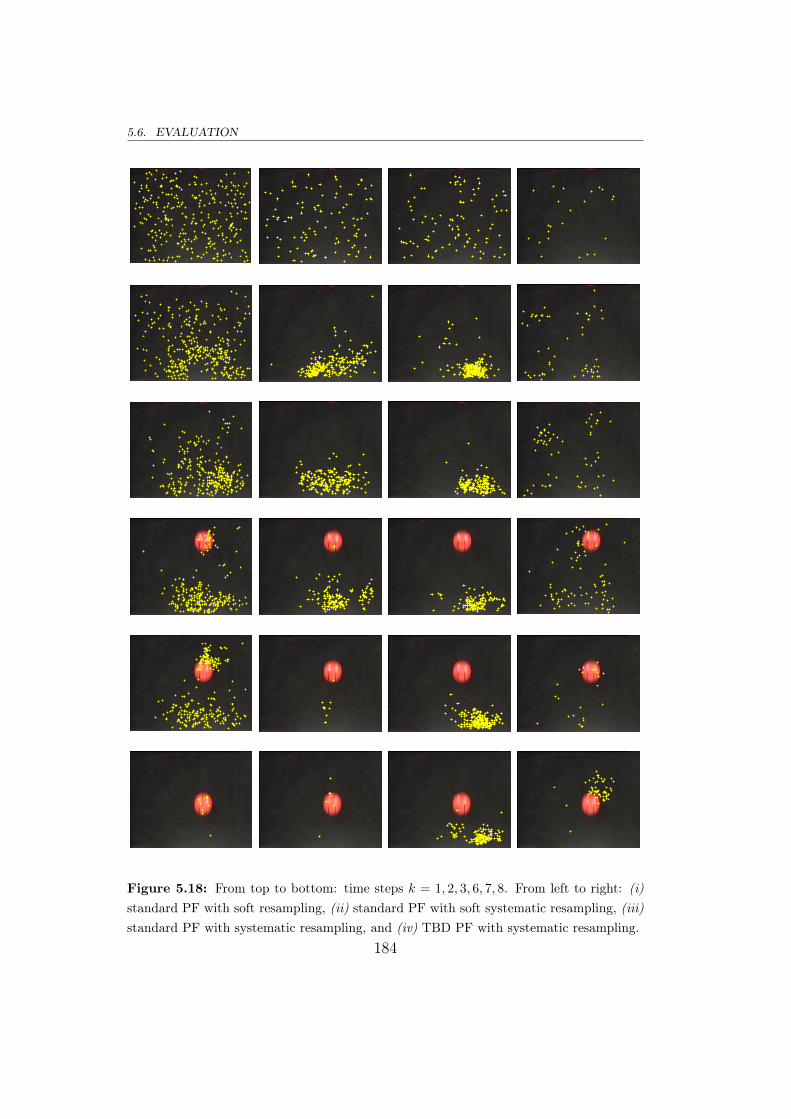
5.6. EVALUATION
Figure 5.18: From top to bottom: time steps k = 1, 2, 3, 6, 7, 8. From left to right: (i)standard PF with soft resampling, (ii) standard PF with soft systematic resampling, (iii)standard PF with systematic resampling, and (iv) TBD PF with systematic resampling.
184

CHAPTER 5. SOFT RESAMPLING
Figure 5.19: From top to bottom: time steps k = 9, 10, 11, 19, 23, 24. From left toright: (i) standard PF with soft resampling, (ii) standard PF with soft systematic resam-pling, (iii) standard PF with systematic resampling, and (iv) TBD PF with systematicresampling. 185

5.7. CONCLUSION AND SUMMARY
5.7 Conclusion and summary
This chapter addressed the role of PF resampling in retaining informationover successive observations and in accurately representing the posterior.State-of-the-art PF resampling schemes do not effectively aid in informationretention over time. Moreover, the standard PF using a conventional resam-pling scheme is not adequate for the detection of covert targets. The TBDPF overcomes this inadequacy but requires an excessive number of particlesto effectively detect new targets. This chapter proposed soft resampling thatproportionally redistributes and reweights the particles so as to preserve theinformation contained in low weights. This chapter also proposed soft sys-tematic resampling that provides means to accurately represent the posteriorand still preserve the low weights. Furthermore, a numerical mechanism thatuses the optimal Kalman filter state estimates in a KS statistic frameworkwas proposed for testing the resampler performance. The key advantagesof the proposed resampling schemes are: a) improved information retentionover time, b) preservation of low weights over time, and b) enhanced posteriorapproximation with fewer particles. The efficacy of the proposed methodswas evaluated using the proposed KS test and in scenarios where retention oflow weights is crucial. Referring back to section 1.3.2 of chapter 1, it can bestated that research goal 3 that aims to overcome problem 3 has been suc-cessfully achieved by the proposed resamplers, and the research goal 4 thataims to overcome problem 4 has been successfully achieved by the proposedKS testing scheme.
186
6Conclusion and future extensions
TTThis dissertation addressed an important research topic in science and en-gineering — the Bayesian multiple target tracking (MTT) [10, 17, 32, 35, 41].Bayesian MTT is useful in many applications. Examples include aircraftand missile tracking using RADAR [1, 152, 154, 158], vessel and fish track-ing using SONAR [2, 99, 100], acoustic and seismic activity tracking [155–157, 192, 214], space debris and spacecraft tracking [3, 106, 107], heart-beattracking from ECG [4, 9, 147], and many others.
This thesis added to the body of knowledge in Bayesian MTT by propos-ing several original innovative ideas that overcome problems with state-of-the-art tracking systems. The central focus of this dissertation is on BayesianMTT from phased sensor array signals [38] using the popular Bayesian ap-proximation tool — the particle filter (PF) [21, 52, 54, 109]. The researchconducted during the course of this thesis investigated and proposed novelsolutions (presented in chapters 3 and 4) that overcame several challenges ofthe focus area — the Bayesian MTT for array signal processing applications
187

6.1. CONTRIBUTIONS OF THIS THESIS
[37]. This research provided further motivation to address and propose lead-ing edge solutions (presented in chapter 5) that overcame challenges of thePF resampling operation.
In this chapter, the thesis contributions and their merits are first sum-marised in section 6.1. Secondly, the research extensions and suggestionsthat could be be addressed in the future are presented in section 6.2. Fi-nally, concluding remarks are presented in section 6.3.
6.1 Contributions of this thesis
In this section, the contributions made by this thesis are summarised.
6.1.1 The MUSIC based MTT PF
Chapter 3 developed the MUltiple SIgnal Classification (MUSIC) based MTTPF, a Bayesian MTT filter for array processing applications.
Motivating problems in contemporary methods: The Bayesian MTTmethod of using a single target filter for each target separately [215, 216] suf-fers from the filter hijack problem [80, 126]. This problem is avoided in thejoint filter [44, 124, 282]. However, the computational complexity in the jointfilter increases significantly with the number of targets [45, 232]. The sub-optimal random finite set (RFS) filters [233] — the probability hypothesisdensity (PHD) filter [26, 32] and the multi-target multi-Bernoulli (MeMBer)filter [31–33, 49, 196], overcome this complexity problem. However, for track-ing targets using phased sensor arrays, they require the sensor signals to befirst converted to an image; this conversion leads to information and resolu-tion loss.
Proposed solution: This thesis proposed the MUSIC based MTT PF, thekey innovation of which is to use for the likelihood function, a proxy which hasas its domain the domain of a single target. The MUSIC pseudo-spectrum is
188

CHAPTER 6. CONCLUSION AND FUTURE EXTENSIONS
such a function. Using MUSIC values as pseudo-weights allow the particlesto operate in the space of a single target. However, tracking multiple targetsin the single target state space results in the eventual convergence of all theparticles around a single target. This problem was overcome by proportion-ally grouping the particles that track each individual target. This groupingwas accomplished by first clustering [59] the particles and then imposing acluster regulation scheme in the subsequent soft resampling [61] stage.
Merits of the proposal: The advantages of the proposed method as com-pared to state-of-the-art methods are as follows; (i) the computational com-plexity is lower than the joint filter by virtue of operating in the single targetspace, (ii) track accuracy is higher than that of the RFS filters by virtueof MUSIC that allows a more direct use of the sensor array data, (iii) closetargets are effectively resolved by virtue of the super resolution property ofMUSIC, and (iv) particle hijack is avoided by virtue of regulated clustering.
6.1.2 The MUSIC based MeMBer filter
Chapter 4 developed the MUSIC based MeMBer filter, a Bayesian RFS filterfor array processing applications.
Motivating problems in contemporary methods: The RFS filters [26,31, 32, 196] operate in the space of a single target and hence are more suit-able for the tracking of many targets. However, they are sub-optimal andtheir performance could be poor at low signal-to-noise ratio (SNR) levels[161, 266]. Moreover, to date, the RFS filters do not possess a suitable mech-anism to operate directly on the phased sensor array signals. This prob-lem can be avoided using image models and image pre-processing techniques[50, 189, 191] which lead to information and resolution loss. Furthermore, inthe “MeMBer filter for beamformer images,” the computation of the beam-former values for all the pixels that fall within a region of influence for eachparticle is computationally expensive.
189

6.1. CONTRIBUTIONS OF THIS THESIS
The proposed solution: This thesis proposed the MUSIC based MeMBerfilter, the key innovation of which is in adapting the MeMBer filter for imageobservations to phased sensor array observations. This is achieved by usingfor the likelihood in the MeMBer filter for image observations, the MUSICpseudo-spectrum — a function which has as its domain the state space of asingle target. The remainder of the algorithm is unchanged.
Merits of the proposal: The simple modification of using MUSIC as aproxy to the likelihood in the MeMBer filter adds considerable merit in itsapplication to array signal processing. The advantages of the method as com-pared to state-of-the-art methods are as follows; (i) improved track accuracyby virtue of using MUSIC which allows the replacement of the image obser-vation with array signals, (ii) lower computational complexity by virtue ofusing MUSIC, i.e., the region of influence is no longer relevant in the proposedtechnique and the filter requires only a single MUSIC value computation foreach particle, and (iii) effective separation of spatially close targets by virtueof the super resolution property of MUSIC.
6.1.3 Soft resampling
Chapter 5 developed the soft and the soft systematic resampling, a PF sub-routine that aids in the replenishment of large weight particles.
Motivating problems in contemporary methods: The conventionalresamplers [52, 54, 118–120, 122] do not effectively aid in information accu-mulation over successive observations. As a result, these resamplers couldeasily eliminate a low weight particle that is gradually acquiring target in-formation. Moreover, the standard PF using a conventional resampler is notsuitable for covert target tracking as such a target need to be tracked forsome duration (i.e., its information need to be retained) before declaring itspresence. This insufficiency is overcome using the track-before-detect (TBD)PF that requires the use of many particles to effectively detect new targets.This requirement increases the computational burden.
190

CHAPTER 6. CONCLUSION AND FUTURE EXTENSIONS
The proposed solution: This thesis proposed soft resampling, the key in-novation of which is the proportional redistribution of particle informationamong all the other particles and the preservation of information containedin the low weight particles. The scheme retains particle information for alonger duration. This thesis also proposed soft systematic resampling (animprovement to soft resampling) that properly treats the tails of the pos-terior. The scheme prevents certain loss of those particles that lie near theboundary of the particle set by stochastically resampling a few lower weightparticles.
Merits of the proposal: The advantages of the proposed methods as com-pared to state-of-the-art methods are as follows; (i) improved informationretention over time, (ii) faster target lock when the target is covert or whenthe prior is not correct, (iii) a more accurate posterior approximation in softsystematic resampling, and (iv) favourable track accuracy.
6.1.4 The KS statistic
Chapter 5 developed a method of practically evaluating the PF approxima-tion error using the well-known Kolmogorov-Smirnov (KS) statistic [273].
Motivating problem: It is known that the PF provides only an approxi-mate representation of the true posterior. A numerical measure to test PFrepresentation accuracy is not available in practice. The PF resampling sub-routine contributes significantly to inaccuracies in PF approximation due tounavoidable particle rejection and replacement operations. Therefore it isimportant to numerically assess the faithfulness of PF resampling in approx-imating the posterior.
The proposed solution: This thesis proposed that the PF accuracy ofposterior representation can be quantitatively evaluated for linear Gaussianmodels in accordance to its Kolmogorov-Smirnov (KS) statistic agreement[273] with the optimal Kalman filter. The KS test is under-utilised in the PF
191

6.2. FUTURE EXTENSIONS OF THIS THESIS
literature and has never been used to measure PF resampling performance.Since KS testing [62, 275, 276] cannot be directly used, this thesis proposedto de-mean and de-correlate the resampled particles using the Kalman meanand covariance. Then the one-sample KS test [62] is conducted along eachdimension separately by comparing the cumulative sum of the (sorted) par-ticle weights and the error function of N (0, 1). Finally, the maximum KSdeviation over all the dimensions is taken. This method was used to test theperformance of the proposed resampler in chapter 5.
Merits of the proposal: If the PF representation is identical to the Kalmanfilter distribution, then the de-mean and de-correlation of particles will resultin a set of uncorrelated particles normally distributed with zero mean andunit variance. Hence the KS deviation of the cumulative distribution func-tion (cdf) of the (sorted) particle weights from the error function of N (0, 1)
will be small. Conversely, if the PF representation is not identical to theKalman filter distribution, then the KS deviation will be large. A numericalmeasure to test the PF representation accuracy is now available in practice.
6.2 Future extensions of this thesis
In this section, the future research extensions and suggestions of this thesisare outlined.
6.2.1 Bayesian filtering for array processing
Some future research ideas identified in the MUSIC based MTT PF proposedin chapter 3 and in the MUSIC based MeMBer filter proposed in chapter 4are now presented.
Hierarchical clustering
This idea relates to the MUSIC based MTT PF presented in chapter 3. Theproposed filter used k-means clustering to group (or separate) the particles so
192

CHAPTER 6. CONCLUSION AND FUTURE EXTENSIONS
as to avoid particle hijack — a general problem that becomes evident whenparticles in the same space try to localise multiple targets. Since the actualnumber of targets is not known, the number of clusters formed is chosen tobe the maximum number of targets the filter can track. A regulation schemeis then imposed to restrict any one cluster from containing more than a fixedproportion of the total number of particles.
An alternative to k-means clustering is the well known hierarchical clus-tering [283] that is known to provide a linkage criterion which specifies thedissimilarity of the particles as a function of their pairwise Euclidean dis-tances. By observing the dendrogram formed by this clustering algorithm(or finding that instance where a certain number of clusters take a long timeto merge), one is able to approximately infer the number of tight clusters, i.e.,the actual number of targets in the scene. The number of clusters formedwould then be approximately equal to the number of actual targets. A clus-ter regulation scheme can then be imposed on these hierarchically clusteredparticles.
Weight based clustering
This idea relates to the MUSIC based MTT PF presented in chapter 3. Theproposed filter used regulated k-means clustering through soft resamplingto avoid particle hijack and to sustain weak targets — targets that gener-ate/reflect weak signals. However, in scenarios where there are only a fewparticles near a weak target, the soft resampler would not replenish suffi-cient particles near that target. As a result, the cluster near the target willcontain an inadequate number of particles. Although these particles (andhence the target) can be sustained by the filter, the track accuracy could beaffected. This problem could be solved by leveraging the clustering proce-dure on the weights of the particles. This can be achieved by replacing thek-means clustering with a method like gravitational clustering [284] whereinthe mass (MUSIC pseudo-weight) of each particle exerts a gravitational at-
193

6.2. FUTURE EXTENSIONS OF THIS THESIS
traction on the nearby masses (weights) such that the particle with a lowermass, although further away, will be eventually attracted to the particle witha higher mass. This will aid in having a sufficient number of particles near aweak target given that the particles further from the target are not trackinganother target. Additionally, this procedure could improve the detection ofcovert targets, especially when the number of targets appearing over time islarge.
Statistical robust signal processing
The ability of the MUSIC based MTT PF of chapter 3 and the MUSIC basedMeMBer filter of chapter 4 to withstand deviations in noise and reverbera-tion model assumptions could be improved using statistical robust signalprocessing [285]. Robust estimation is known to successfully handle situa-tions where the actual system parameters deviate widely from their assumeddistributions. Using the robust MUSIC algorithm presented in [286, 287],the possibility of developing a robust-MUSIC based MTT PF and a robust-MUSIC based MeMBer filter could be investigated.
MUSIC as observation in RFS filters
The MTT filters in chapters 3 and 4 that were designed to operate in singletarget space used MUSIC as a proxy for the likelihood function. This ap-proach facilitated in accelerating the filtering process and in resolving closetargets more effectively. An alternative approach is to use a MUSIC image asthe observation feed to the RFS filters. The applicability of this idea couldbe tested comprehensively.
6.2.2 ESPRIT based measurement feed for PHD filter
Another research suggestion relating to Bayesian MTT using phased sensorarrays is now presented. It is known that the observation feed to the PHD
194

CHAPTER 6. CONCLUSION AND FUTURE EXTENSIONS
filter can only be a finite set of point target detections. This impedes the di-rect use of the filter on array data. This impediment is usually circumventedby a two-stage conversion process; a) converting the array signals into images[50, 189, 191], and b) pre-processing [192] the images to obtain the observa-tion feed. This procedure causes a two-stage information loss.
An alternative approach to convert the array data (that has not beenexplored in the literature) is as follows. For array processing localisationapplications, the well known estimation of signal parameters via rotationalinvariant techniques (ESPRIT) [288, 289] algorithm provides point estimateslike positions, angles of arrival (AOA), etc., directly from the array data.These ESPRIT estimates can be used as the observation feed to the PHD fil-ter. The advantage of this proposition is that there is a more direct use of thearray data because the conversion is now single-stage. This could improvethe filter accuracy at low SNR. However, the ESPRIT algorithm requires theknowledge about the actual number of targets to obtain the eigenvectors thatlie in the signal space. One approach to address this requirement is to usethe minimum-mean-square-error (MMSE) based minimum description length(MDL) algorithm [258] (described and used in section 3.5.2 of chapter 3). Asecond approach is as follows: the ESPRIT algorithm can localise at mostM− 1 targets, where M is the number of sensors. If the algorithm is directedto generate M − 1 target estimates, then (M − 1) − N (let N be the actualnumber of targets) of these estimates would be incorrect (false) detections.The PHD filter will eliminate these false detection peaks as time progresses,provided that the false detections are independent from one time to the next.The possibility of operating the PHD filter with its observation feed beingthe ESPRIT output estimates could be investigated. The idea could be ex-tended to the well known root-MUSIC [246] algorithm which also generatespoint estimates about the target states. Moreover, the time independency offalse detections generated by ESPRIT could also be investigated.
195
6.3. CONCLUSION
6.3 Conclusion
The central focus of this dissertation is on Bayesian MTT using PFs for arrayprocessing applications. This dissertation addressed several challenges ofstate-of-the-art methods in; a) Bayesian filtering for array processing, and b)PF resampling. This concluding chapter first summarised the contributionsmade by this thesis and then outlined research extensions and ideas whichcould be investigated in the future.
196

Bibliography
[1] M. V. Finn, “Unified data fusion applied to monopulse tracking,” DTICDocument, Tech. Rep., 1999.
[2] A. Xydes, M. Moline, C. Lowe, T. J. Farrugia, and C. Clark, “Behav-ioral characterization and particle filter localization to improve tempo-ral resolution and accuracy while tracking acoustically tagged fishes,”J. Elsevier Ocean Engineering, vol. 61, pp. 1–11, 2013.
[3] J. Huang and W. Hu, “MCMC-Particle-based group tracking of spaceobjects within Bayesian framework,” J. Elsevier Adv. in Space Re-search, vol. 53, no. 2, pp. 280–294, 2014.
[4] S. H. Salleh, H. S. Hussain, T. T. Swee, C. M. Ting, A. M. Noor,S. Pipatsart, J. Ali, and P. P. Yupapin, “Acoustic cardiac signals anal-ysis: a Kalman filter-based approach.” J. Nanomedicine, vol. 7, pp.2873–2881, 2011.
[5] Y. Bar Shalom, Tracking and data association. Academic Press Pro-fessional, Inc., 1987.
[6] E. Ozkan, C. Lundquist, and F. Gustafsson, “A Bayesian approach tojointly estimate tire radii and vehicle trajectory,” in Proc. IEEE Intell.Transp. Syst., 2011, pp. 1622–1627.
[7] C. Fernández-Prades, P. Closas, and J. Fernández-Rubio, “Rao-Blackwellized variable rate particle filtering for handset tracking in
197
BIBLIOGRAPHY
communication and sensor networks,” in Proc. European Signal Pro-cess., 2007, pp. 111–115.
[8] A. Rahni, K. Wells, E. Lewis, M. Guy, and B. Goswami, “An iterativeparticle filter approach for respiratory motion estimation in nuclearmedicine imaging,” in Proc. SPIE Medical Imaging, 2011, pp. 79 624C–79 624C.
[9] B. Balasingam, M. Forouzanfar, M. Bolić, H. Dajani, V. Groza, andS. Rajan, “Arterial blood pressure parameter estimation and trackingusing particle filters,” in Proc. IEEE Med. Meas. and Appl., 2011, pp.473–476.
[10] Y. B. Shalom, X. R. Li, and T. Kirubarajan, Estimation with applica-tions to tracking and navigation: theory algorithms and software. JohnWiley & Sons, 2004.
[11] S. S. Blackman and R. Popoli, Design and analysis of modern trackingsystems. Artech House Norwood, 1999, vol. 685.
[12] A. F. M. Smith and A. E. Gelfand, “Bayesian statistics without tears:A sampling–resampling perspective,” Am. Statist., vol. 46, no. 2, pp.84–88, 1992.
[13] W. Bolstad, Introduction to Bayesian statistics. WILEY-INTERSCIENCE, 2004.
[14] S. R. Eddy, “What is Bayesian statistics?” J. Nature Biotechnology,vol. 22, no. 9, pp. 1177–1178, 2004.
[15] D. Koller and N. Friedman, Probabilistic graphical models: principlesand techniques. The MIT Press, 2009.
[16] T. Bayes and Price, “An essay towards solving a problem in the Doc-trine of Chances. By the late Rev. Mr. Bayes, FRS communicated by
198

BIBLIOGRAPHY
Mr. price, in a letter to John Canton, AMFRS,” Trans. Royal SocietyPhilosophical, vol. 53, pp. 370–418, 1763.
[17] T. Bayes, D. Bunn, H. Raiffa, R. Schlaifer, and D. Winterfeldt, “An es-say toward solving a problem in the doctrine of chances,” PhilosophicalTrans. Royal Society London, vol. 53, 1984.
[18] A. Papoulis and S. U. Pillai, Probability, random variables, and stochas-tic processes. Tata McGraw-Hill Education, 2002.
[19] Y. C. Ho and R. Lee, “A Bayesian approach to problems in stochasticestimation and control,” IEEE Trans. Automatic Control, vol. 9, no. 4,pp. 333–339, 1964.
[20] R. E. Kalman, “A new approach to linear filtering and prediction prob-lems,” J. Basic Engineering, vol. 82, no. 1, pp. 35–45, 1960.
[21] N. J. Gordon, D. J. Salmond, and A. F. M. Smith, “Novel approachto non-linear/non-Gaussian Bayesian state estimation,” in Proc. Inst.Elect. Eng., vol. 140, no. 2, 1993, pp. 107–113.
[22] N. Metropolis and S. Ulam, “The Monte Carlo method,” J. Am. Sta-tistical Association, vol. 44, no. 247, pp. 335–341, 1949.
[23] N. Metropolis, A. W.Rosenbluth, M. N. Rosenbluth, A. H. Teller, andE. Teller, “Equation of state calculations by fast computing machines,”J. Chemical Physics, vol. 21, no. 6, pp. 1087–1092, 1953.
[24] J. E. Handschin and D. Q. Mayne, “Monte Carlo techniques to esti-mate the conditional expectation in multi-stage non-linear filtering,” J.Control, vol. 9, no. 5, pp. 547–559, 1969.
[25] J. E. Handschin, “Monte Carlo techniques for prediction and filtering ofnon-linear stochastic processes,” J. Elsevier Automatica, vol. 6, no. 4,pp. 555–563, 1970.
199

BIBLIOGRAPHY
[26] R. P. S. Mahler, “Multitarget Bayes filtering via first-order multitargetmoments,” IEEE Aerosp. Electron. Syst. Mag., vol. 39, no. 4, pp. 1152–1178, 2003.
[27] S. Mori, C. Y. Chong, E. Tse, and R. P. Wishner, “Tracking and classi-fying multiple targets without identification,” IEEE Trans. AutomaticControl, vol. 31, no. 5, pp. 401–409, 1986.
[28] I. R. Goodman, Mathematics of data fusion. Springer, 1997, vol. 37.
[29] J. Goutsias, R. P. S. Mahler, and H. T. Nguyen, Random Sets: Theoryand Applications. Springer New York, 1997.
[30] H. Fei and I. Reid, “Joint Bayes filter: A hybrid tracker for non-rigidhand motion recognition,” in J. Springer Computer Vision, 2004, pp.497–508.
[31] B. T. Vo, B. N. Vo, and A. Cantoni, “The cardinality balanced multi-target multi-Bernoulli filter and its implementations,” IEEE Trans.Signal Process., vol. 57, no. 2, pp. 409–423, 2009.
[32] R. P. S. Mahler, Statistical Multisource-Multitarget Information Fusion.Artech House Publishers, 2007, vol. 685.
[33] B. T. Vo, B. N. Vo, and A. Cantoni, “On multi-Bernoulli approxima-tions to the Bayes multi-target filter,” in Proc. Inf. Fusion, 2007.
[34] R. P. S. Mahler, “ “Statistics 101” for multisensor, multitarget datafusion,” IEEE Aerosp. and Electron. Syst. Mag., vol. 19, no. 1, pp.53–64, 2004.
[35] L. D. Stone, C. A. Barlow, and T. L. Corwin, Bayesian multiple targettracking. Artech House, 1999.
[36] L. D. Stone, R. L. Streit, T. L. Corwin, and K. L. Bell, Bayesianmultiple target tracking. Artech House, 2013.
200

BIBLIOGRAPHY
[37] D. H. Johnson and D. E. Dudgeon, Array signal processing: conceptsand techniques. Simon & Schuster Pub., 1992.
[38] M. Viberg and B. Ottersten, “Sensor array processing based on sub-space fitting,” IEEE Trans. on Signal Process., vol. 39, no. 5, pp. 1110–1121, 1991.
[39] M. R. Bai, A. Agarwal, C. C. Chen, and Y. C. Wang, “Bayesianapproach of nearfield acoustic reconstruction with particle filters,” J.Acoust. Soc. of America, vol. 133, no. 6, pp. 4032–4043, 2013.
[40] B. A. Yocom, J. M. Aughenbaugh, and B. R. L. Cour, “Range-sensitiveBayesian passive sonar tracking,” in Proc. Inf. Fusion, 2010, pp. 1–10.
[41] V. Trees and L. Harry, Detection, Estimation, and Modulation theory.John Wiley & Sons, 2004.
[42] D. Avitzour, “Stochastic simulation Bayesian approach to multitargettracking,” in Proc. IEE Radar, Sonar and Navig., vol. 142, no. 2, 1995,pp. 41–44.
[43] T. E. Fortmann, Y. Bar-Shalom, and M. Scheffe, “Multi-target trackingusing joint probabilistic data association,” in Proc. IEEE Decision andControl Adaptive Process., vol. 19, 1980, pp. 807–812.
[44] C. Kreucher, K. Kastella, and A. O. Hero III, “Multitarget trackingusing the joint multitarget probability density,” IEEE Trans. Aerosp.Electron. Syst., vol. 41, no. 4, pp. 1396–1414, 2005.
[45] F. Daum and J. Huang, “Curse of dimensionality and particle filters,”in Proc. IEEE Aerosp. Conf., 2003, pp. 1979–1993.
[46] T. Bengtsson, P. Bickel, and B. Li, “Curse-of-dimensionality revisited:Collapse of the particle filter in very large scale systems,” in J. IMSProbability and Statistics, 2008, vol. 2, pp. 316–334.
201

BIBLIOGRAPHY
[47] W. Yi, M. Morelande, L. Kong, and J. Yang, “A computationally ef-ficient particle filter for multi-target tracking using an independenceapproximation,” IEEE Trans. on Signal Process., vol. 61, no. 4, pp.843–856, 2013.
[48] J. Vermaak, S. J. Godsill, and P. Pérez, “Monte Carlo filtering formulti target tracking and data association,” IEEE Aerosp. Electron.Syst., vol. 41, no. 1, pp. 309–332, 2005.
[49] B. N. Vo, B. T. Vo, N. T. Pham, and D. Suter, “Bayesian multi-objectestimation from image observations,” in Proc. Inf. Fusion, 2009, pp.890–898.
[50] D. E. Clark, I. T. Ruiz, Y. Petillot, and J. Bell, “Particle PHD filtermultiple target tracking in sonar image,” IEEE Aerosp. Electron. Syst.,vol. 43, no. 1, pp. 409–416, 2007.
[51] M. Tobias and A. D. Lanterman, “Techniques for birth-particle place-ment in the probability hypothesis density particle filter applied topassive radar,” Proc. IET Radar, Sonar & Navig., vol. 2, no. 5, pp.351–365, 2008.
[52] S. Arulampalam, S. Maskell, N. Gordon, and T. Clapp, “A tutorial onparticle filters for online nonlinear/non-gaussian Bayesian tracking,”IEEE Trans. Signal Process., vol. 50, no. 2, pp. 174–188, 2002.
[53] J. Liu and R. Chen, “Sequential Monte Carlo Methods for DynamicSystems,” Journal of the American Statistical Association, vol. 93, pp.1032–1044, 1998.
[54] P. M. Djurić, J. H. Kotecha, J. Zhang, Y. Huang, T. Ghirmai, M. F.M. Bugallo, and J. Miguez, “Particle filtering,” IEEE Signal Process.Mag., vol. 20, no. 5, pp. 19–38, 2003.
[55] D. J. Salmond and H. Birch, “A particle filter for track-before-detect,”in Proc. IEEE American Control Conf., vol. 5, 2001, pp. 3755–3760.
202

BIBLIOGRAPHY
[56] B. Ristic, S. Arulampalam, and N. Gordon, Beyond the Kalman Filter:Particle Filters for Tracking Applications. Artech House Publishers,2004.
[57] R. Schmidt, “Multiple emitter location and signal parameter estima-tion,” IEEE Trans. Antennas Propag., vol. 34, no. 3, pp. 276–280, 1986.
[58] J. MacQueen, “Some methods for classification and analysis of mul-tivariate observations,” in Proc. Berkeley Symp. Mathematical Statist.and Probability, vol. 1, no. 281-297, 1967, p. 14.
[59] J. A. Hartigan, Clustering algorithms. John Wiley & Sons, Inc., 1975.
[60] J. Friedman, T. Hastie, and R. Tibshirani, The Elements of StatisticalLearning. Springer Series in Statistics, 2001, vol. 2, no. 1.
[61] P. B. Choppala, P. D. Teal, and M. R. Frean, “Soft resampling forimproved information retention in particle filtering,” in Proc. IEEE Int.Conf. Acoust., Speech, Signal Process., vol. 13, 2013, pp. 4036–4040.
[62] J. A. Peacock, “Two-dimensional goodness-of-fit testing in astronomy,”Royal Astronomical Society, vol. 202, pp. 615–627, 1983.
[63] S. M. Kay, “Fundamentals of statistical signal processing: Detectiontheory,” 1998.
[64] A. H. Jazwinski, “Stochastic processes and filtering theory,” Mathemat-ics in Science and Eng., no. 64, 1970.
[65] B. P. Carlin, N. G. Polson, and D. S. Stoffer, “A Monte Carlo approachto nonnormal and nonlinear state-space modeling,” J. Am. StatisticalAsso., vol. 87, no. 418, pp. 493–500, 1992.
[66] W. Zhang, State-space search: Algorithms, complexity, extensions, andapplications. Springer, 1999.
203

BIBLIOGRAPHY
[67] C. W. Gardiner et al., Handbook of stochastic methods. Springer Berlin,1985, vol. 3.
[68] Z. Ghahramani, “An introduction to hidden Markov models andBayesian networks,” J. World Scientific Pattern Recog. Artificial In-tell., vol. 15, no. 01, pp. 9–42, 2001.
[69] J. Burlet, T. D. Vu, and O. Aycard, “Grid-based localization and onlinemapping with moving object detection and tracking,” 2007.
[70] K. Kastella, “Event-averaged maximum likelihood estimation andmean-field theory in multitarget tracking,” IEEE Trans. AutomaticControl, vol. 40, no. 6, pp. 1070–1074, 1995.
[71] C. M. Kreucher, K. D. Kastella, and A. O. Hero III, “Tracking multipletargets using a particle filter representation of the joint multitargetprobability density,” in Proc. SPIE, Optical Science and Technology,2003, pp. 258–269.
[72] K. D. Kastella, “Joint multitarget probabilities for detection and track-ing,” in SPIE Proc. AeroSense. International Society for Optics andPhotonics, 1997, pp. 122–128.
[73] D. Avitzour, “A maximum likelihood approach to data association,”IEEE Trans. Aerosp. and Electron. Syst., vol. 28, no. 2, pp. 560–566,1992.
[74] D. Reid, “An algorithm for tracking multiple targets,” IEEE Trans. onAutomatic Control, vol. 24, no. 6, pp. 843–854, 1979.
[75] R. E. Bellman, “Dynamic programming and Lagrange multipliers,”Proc. National Academy Sciences, vol. 42, no. 10, p. 767, 1956.
[76] ——, Adaptive control processes: A guided tour. Princeton UniversityPress, 1961, vol. 4.
204

BIBLIOGRAPHY
[77] N. Weiner, Extrapolation, interpolation, and smoothing of stationarytime series: with engineering applications, vol. 8.
[78] G. Welch and G. Bishop, “An introduction to the Kalman filter,” Tech.Rep., 1995.
[79] M. S. Grewal and A. P. Andrews, Kalman filtering: Theory and prac-tice. Prentice Hall, 1993.
[80] A. Bhatia, “Hierarchical Charged Particle Filter for Multiple TargetTracking,” Ph.D. dissertation, North Carolina State University, 2012.
[81] R. E. Kalman and R. S. Bucy, “New results in linear filtering andprediction theory,” J. Basic Eng., vol. 83, no. 1, pp. 95–108, 1961.
[82] J. George, “Robust Kalman-Bucy filter,” IEEE Trans. Automatic Con-trol, vol. 58, no. 1, pp. 174–180, 2013.
[83] R. Lefferts, “Altitude estimation using asynchronous α-β tracking fil-ters,” IEEE Trans. Aerosp. and Electron. Syst., no. 4, pp. 469–477,1982.
[84] P. R. Kalata, “The tracking index: A generalized parameter for Alpha-Beta and Alpha-Beta-Gamma target trackers,” IEEE Tran. Aerosp.Electron. Syst., no. 2, pp. 174–182, 1984.
[85] S. F. Schmidt, “Application of state-space methods to navigation prob-lems,” J. Adv. Control Syst., vol. 3, pp. 293–340, 1966.
[86] V. E. Beneš, “New exact nonlinear filters with large Lie algebras,” J.Elsevier Systems & Control Lett., vol. 5, no. 4, pp. 217–221, 1985.
[87] F. E. Daum, “New exact nonlinear filters,” Proc. Bayesian Analysis ofTime Series and Dynamic Models, vol. 94, pp. 199–226, 1988.
[88] L. A. Zadeh, “Optimum nonlinear filters,” J. Applied Physics, vol. 24,no. 4, pp. 396–404, 2004.
205

BIBLIOGRAPHY
[89] D. Simon, Optimal state estimation: Kalman, H infinity, and nonlinearapproaches. John Wiley & Sons, 2006.
[90] F. Gustafsson and G. Hendeby, “Some relations between extended andunscented Kalman filters,” IEEE Trans. on Signal Process., no. 99, pp.545–555, 2012.
[91] H. Tanizaki and R. S. Mariano, “Nonlinear filters based on Taylorseries expansions,” Comm. Stat. Theory and Methods, vol. 25, no. 6,pp. 1261–1282, 1996.
[92] S. J. Julier and J. K. Uhlmann, “A new extension of the Kalman filterto nonlinear systems,” in Proc. Int. Symp. Aerosp./Ddefense Sensing,Simul. and Controls, vol. 3, no. 26, 1997, pp. 3–2.
[93] ——, “A general method for approximating nonlinear transformationsof probability distributions,” Tech. Rep., 1996.
[94] ——, “Unscented filtering and nonlinear estimation,” Proc. IEEE,vol. 92, no. 3, pp. 401–422, 2004.
[95] E. Wan and R. V. D. Merwe, “The unscented Kalman filter for nonlin-ear estimation,” in Proc. IEEE Adaptive Systems for Signal Process.,Comm., and Control, 2000, pp. 153–158.
[96] F. Gustafsson and G. Hendeby, “On nonlinear transformations ofstochastic variables and its application to nonlinear filtering,” in Proc.IEEE Acoustic., Speech and Signal Proc., 2008, pp. 3617–3620.
[97] T. Kailath, A. H. Sayed, and B. Hassibi, “Linear estimation,” 2000.
[98] T. I. Fossen and T. Perez, “Kalman filtering for positioning and headingcontrol of ships and offshore rigs,” IEEE Control Syst. Mag., vol. 29,no. 6, pp. 32–46, 2009.
206

BIBLIOGRAPHY
[99] D. B. Cousins, “Underwater model-based processing for SLAM andenvironment characterization,” in Proc. IEEE Aerosp., 2008, pp. 1–10.
[100] K. S. Rao, “Pseudo linear Kalman filter for underwater target locationusing intercept sonar measurements,” in Proc. IEEE Position, locationand navig., 2006, pp. 1036–1039.
[101] S. Chumchean, A. Seed, and A. Sharma, “Correcting of real-time radarrainfall bias using a Kalman filtering approach,” J. Elsevier Hydrology,vol. 317, no. 1, pp. 123–137, 2006.
[102] D. Carevic, “Kalman filter-based approach to target detection andtarget-background separtion in ground-penetrating radar data,” inProc. ISOP AeroSense, 1999, pp. 1284–1288.
[103] C. Yardim, P. Gerstoft, and W. S. Hodgkiss, “Tracking of geoacousticparameters using Kalman and particle filters,” J. Acoust. Soc. Am.,vol. 125, no. 2, pp. 746–760, 2009.
[104] X. Deng and J. Hu, “A new Kalman filter for tracking event of seismicrecord,” in Proc. IEEE Image Signal Process., no. 13, 2013, pp. 1143–1147.
[105] J. Traa and P. Smaragdis, “A wrapped Kalman filter for azimuthalspeaker tracking,” IEEE Signal Process. Lett., vol. 20, no. 12, pp. 1257–1260, 2013.
[106] E. J. Lefferts, F. L. Markley, and M. D. Shuster, “Kalman filtering forspacecraft attitude estimation,” J. Guidance, Control, and Dynamics,vol. 5, no. 5, pp. 417–429, 1982.
[107] M. T. Nasri and W. Kinsner, “Extended Kalman filtering for pico-satellites attitude determination,” in Proc. IEEE Elec. Comp. Eng.,2013, pp. 1–5.
207

BIBLIOGRAPHY
[108] G. Kitagawa, “Non-Gaussian state-space modeling of non-stationarytime series,” J. Am. Statist. Asso., vol. 82, no. 400, pp. 1032–1041,1987.
[109] A. Doucet, N. D. Freitas, and N. Gordon, An introduction to SequentialMonte Carlo methods in practice. Springer New York, 2001, vol. 1.
[110] A. Doucet, S. J. Godsill, and C. Andrieu, “On sequential Monte Carlosampling methods for Bayesian filtering,” J. Springer Statistic. Com-puting, vol. 10, no. 3, pp. 197–208, 2000.
[111] S. J. Godsill, A. Doucet, and M. West, “Monte Carlo smoothing fornonlinear time series,” J. Am. Statist. Asso., vol. 99, no. 465, 2004.
[112] M. Carter and B. V. Brunt, The Lebesgue-Stieltjes integral. Springer.
[113] J. R. Blum, D. L. Hanson, and L. H. Koopmans, “On the strong lawof large numbers for a class of stochastic processes,” J. Springer Prob-ability Theory and Related Fields, vol. 2, no. 1, pp. 1–11, 1963.
[114] Z. Chen, “Bayesian filtering: From Kalman filters to particle filters,and beyond,” J. Statistics, vol. 182, no. 1, pp. 1–69, 2003.
[115] T. K. Chandra, “Uniform integrability in the Cesaro sense and theweak law of large numbers,” J. Indian Statistics, pp. 309–317, 1989.
[116] D. Crisan and A. Doucet, “A survey of convergence results on parti-cle filtering methods for practitioners,” IEEE Tran. Signal Process.,vol. 50, no. 3, pp. 736–746, 2002.
[117] X. L. Hu, T. Schön, and L. Ljung, “A basic convergence result forparticle filtering,” IEEE Tran. Signal Process., vol. 56, no. 4, pp. 1337–1348, 2008.
[118] J. D. Hol, T. B. Schön, and F. Gustafsson, “On Resampling Algorithmsfor Particle Filters,” in Proc. Nonlinear Stat. Signal Process. Workshop,2006.
208

BIBLIOGRAPHY
[119] R. Douc and O. Cappé, “Comparison of resampling schemes for particlefiltering,” in Proceedings ISPA 4th International Symposium on Imageand Signal Processing and Analysis, 2005, pp. 64–69.
[120] M. Bolić, P. M. Djurić, and S. Hong, “Resampling algorithms for par-ticle filters: A computational complexity perspective,” J. EURASIPApplied Signal Process., vol. 2004, pp. 2267–2277, 2004.
[121] J. D. Hol, “Resampling in particle filters,” Tech. Rep., 2004.
[122] M. Bolić, P. M. Djurić, and S. Hong, “Resampling algorithms and archi-tectures for distributed particle filters,” IEEE Trans. Signal Process.,vol. 53, no. 7, pp. 2442–2450, 2005.
[123] K. Pearson, “The problem of the random walk,” J. Nature, vol. 72, no.1865, p. 294, 1905.
[124] M. R. Morelande, C. M. Kreucher, and K. Kastella, “A Bayesian ap-proach to multiple target detection and tracking,” IEEE Trans. SignalProcess., vol. 55, no. 5, pp. 1589–1604, 2007.
[125] W. Du and J. Piater, “Tracking by cluster analysis of feature pointsand multiple particle filters,” Pattern Recognition and Image Analysis,pp. 701–710, 2005.
[126] J. Vermaak, A. Doucet, and P. Pérez, “Maintaining multimodalitythrough mixture tracking,” in Proc. IEEE 9th Int. Conf. ComputerVision, 2003, pp. 1110–1116.
[127] M. Orton and W. Fitzgerald, “A Bayesian approach to tracking multi-ple targets using sensor arrays and particle filters,” IEEE Trans. SignalProcess., vol. 50, no. 2, pp. 216–223, 2002.
[128] A. Giremus, J. Tourneret, and P. Djuric, “An improved regularizedparticle filter for gps/ins integration,” in Proc. IEEE Signal Process.Adv. Wireless Comm., 2005, pp. 1013–1017.
209

BIBLIOGRAPHY
[129] N. Vaswani and D. Das, “Particle filter with efficient importance sam-pling and mode tracking (pf-eis-mt) and its application to landmarkshape tracking,” in Proc. IEEE Signals, Syst. and Computers, 2007,pp. 720–724.
[130] N. Yang, B. Ding, and J. Zhang, “Improved sampling importance re-sampling particle filter optimized by Tabu search,” in Proc. IEEE Ar-tificial Intell. and Comput. Intell., vol. 3, 2010, pp. 359–363.
[131] C. Shen, D. A. H. Hengel, B. Anthony, and M. J. Brooks, “Enhancedimportance sampling: Unscented auxiliary particle filtering for visualtracking,” in J. Springer Adv. in Artificial Intell., 2005, pp. 180–191.
[132] P. Torma and C. Szepesvári, “Local importance sampling: A noveltechnique to enhance particle filtering,” J. Multimedia, vol. 1, no. 1,pp. 32–43, 2006.
[133] M. Rollason and D. Salmond, “A particle filter for track-before-detectof a target with unknown amplitude,” in Proc. IEE Target Tracking:Algorithms and Applications, vol. 1, 2001, pp. 14/1–14/4.
[134] M. Fallon and S. J. Godsill, “Multi target acoustic source tracking usingtrack before detect,” in Proc. IEEE Workshop Appl. of Signal Process.to Audio and Acoust., 2007, pp. 102–105.
[135] M. K. Pitt and N. Shephard, “Filtering via simulation: Auxiliary par-ticle filters,” J. of the American Statistical Association, pp. 590–599,1999.
[136] J. Carpenter, P. Clifford, and P. Fearnhead, “An improved particle filterfor nonlinear problems,” Proc. IEE Radar, Sonar and Navigation, vol.146, pp. 2–7, 1999.
[137] D. Ustebay, M. Coates, and M. Rabbat, “Distributed auxiliary particlefilters using selective gossip,” in Proc. IEEE Acoust., Speech and SignalProcess., 2011, pp. 3296–3299.
210

BIBLIOGRAPHY
[138] G. Johannesson, B. Hanley, and J. Nitao, “Dynamic Bayesian modelsvia Monte Carlo–An introduction with examples,” Lawrence LivermoreNational Laboratory, UCRL-TR-207173, 2004.
[139] R. V. D. Merwe, A. Doucet, N. D. Freitas, and E. Wan, “The unscentedparticle filter,” Adv. Neural Inf. Process. Systems, pp. 584–590, 2001.
[140] L. Xue, S. Gao, and J. Wang, “Research on robust unscented regular-ized particle filtering,” in Proc. IEEE Inf. Theory Inf. Security, 2010,pp. 790–793.
[141] C. Andrieu, N. D. Freitas, A. Doucet, and M. Jordan, “An introductionto MCMC for machine learning,” J. Machine Learning, vol. 50, no. 1,2003.
[142] M. R. Morelande, “A marginalised particle filter for bearings-onlytracking,” in Proc. IEEE Acoust., Speech and Signal Process., 2013,pp. 6298–6302.
[143] T. Schön, F. Gustafsson, and P. J. Nordlund, “Marginalized particlefilters for mixed linear/nonlinear state-space models,” IEEE Trans.Signal Process., vol. 53, no. 7, pp. 2279–2289, 2005.
[144] N. D. Freitas, “Rao-Blackwellised particle filtering for fault diagnosis,”in Proc. IEEE Aerosp., vol. 4, 2002, pp. 4/1767–4/1772.
[145] P. Nordlund and F. Gustafsson, “Marginalized particle filter for accu-rate and reliable terrain-aided navigation,” IEEE Trans. Aerosp. andElectron. Systems, vol. 45, no. 4, pp. 1385–1399, 2009.
[146] C. Fritsche, T. Schon, and A. Klein, “The marginalized auxiliary parti-cle filter,” in Proc. IEEE Comput. Adv. Multi-Sensor Adaptive Process.,2009, pp. 289–292.
[147] P. D. Teal, “Bayesian phase tracking for multiple pulse signals,” J.Elsevier Signal Process., vol. 90, no. 6, pp. 2050–2059, 2010.
211

BIBLIOGRAPHY
[148] Y. Boers and J. N. Driessen, “Interacting multiple model particle filter,”Proc. IEE Radar, Sonar and Navig., vol. 150, no. 5, pp. 344–349, 2003.
[149] L. Hong, N. Cui, M. Bakich, and J. R. Layne, “Multirate interactingmultiple model particle filter for terrain-based ground target tracking,”in Proc. IEE Control Theory and Appl., vol. 153, no. 6, 2006, pp. 721–731.
[150] F. Maurelli, Y. Petillot, A. Mallios, P. Ridao, and S. Krupinski, “Sonar-based AUV localization using an improved particle filter approach,” inProc. IEEE Oceans, 2009, pp. 1–9.
[151] C. V. S. Rodrigues and W. S. Filho, “Particle filter applied in the real-time bearings-only tracking problem of a sonar target,” in Proc. Acout.,2008, pp. 2453–2458.
[152] Y. Boers and J. N. Driessen, “Multitarget particle filter track beforedetect application,” in Proc. IEE Radar, Sonar and Navig., vol. 151,no. 6, 2004, pp. 351–357.
[153] X. Deng, Y. Pi, M. R. Morelande, and B. Moran, “Track-before-detectprocedures for low pulse repetition frequency surveillance radars,” Proc.IET Radar, Sonar & Navig., vol. 5, no. 1, pp. 65–73, 2011.
[154] G. Li, R. Ebelt, and M. Vossiek, “Particle filter based synthetic aperturereconstruction approach for real-time 3D wireless local positioning,” inProc. IEEE Microwave, 2012, pp. 1–4.
[155] A. M. Johansson, E. A. Lehmann, and S. Nordholm, “Real-time imple-mentation of a particle filter with integrated voice activity detector foracoustic speaker tracking,” in Proc. IEEE Circuits and Systems, 2006,pp. 1004–1007.
[156] C. Andrieu and S. J. Godsill, “A particle filter for model based audiosource separation,” in Proc. Workshop Independent Component Analy-sis, 2000.
212
BIBLIOGRAPHY
[157] E. Baziw, “Real-time seismic signal enhancement utilizing a hybridRao-Blackwellized particle filter and hidden Markov model filter,”IEEE Geoscience and Remote Sensing Lett., vol. 2, no. 4, pp. 418–422, 2005.
[158] A. Benavoli, L. Chisci, and A. Farina, “Tracking of a ballistic missilewith a-priori information,” IEEE Trans. Aerosp. and Electron. Syst.,vol. 43, no. 3, pp. 1000–1016, 2007.
[159] Y. Zhou, E. Yeniaras, P. Tsiamyrtzis, N. Tsekos, and I. Pavlidis, “Col-laborative tracking for MRI-guided robotic intervention on the beat-ing heart,” in J. Springer Medical Image Computing and Computer-Assisted Intervention, 2010, pp. 351–358.
[160] F. Gustafsson, F. Gunnarsson, N. Bergman, U. Forssell, J. Jansson,R. Karlsson, and P. J. Nordlund, “Particle filters for positioning, nav-igation, and tracking,” IEEE Tran. Signal Process., vol. 50, no. 2, pp.425–437, 2002.
[161] H. Sidenbladh, “Multi-target particle filtering for the probability hy-pothesis density,” in Proc. Inf. Fusion, vol. 2, 2003, pp. 800–806.
[162] T. Zajic and R. P. S. Mahler, “Particle-systems implementation of thePHD multitarget-tracking filter,” in Proc. SPIE, vol. 5096, 2003, pp.291–299.
[163] B. N. Vo, S. Singh, and A. Doucet, “Sequential Monte Carlo imple-mentation of the PHD filter for multi-target tracking,” in Proc. Inf.Fusion, 2003, pp. 792–799.
[164] E. Maggio, E. Piccardo, C. Regazzoni, and A. Cavallaro, “ParticlePHD filtering for multi-target visual tracking,” in Proc. IEEE Acoust.,Speech and Signal Process., vol. 1, 2007, pp. I–1101.
213

BIBLIOGRAPHY
[165] N. Whiteley, S. Singh, and S. J. Godsill, “Auxiliary particle implemen-tation of probability hypothesis density filter,” IEEE Tran. Aerosp.and Electron. Syst., vol. 46, no. 3, pp. 1437–1454, 2010.
[166] E. Baser and M. Efe, “A novel auxiliary particle PHD filter,” in Proc.Inf. Fusion, 2012, pp. 165–172.
[167] A. M. Johansen, S. Singh, A. Doucet, and B. N. Vo, “Convergence ofthe SMC implementation of the PHD filter,” J. Springer Methodologyand Computing in Applied Probability, vol. 8, no. 2, pp. 265–291, 2006.
[168] D. E. Clark and J. Bell, “Convergence results for the particle PHDfilter,” IEEE Trans. Signal Process., vol. 54, no. 7, pp. 2652–2661,2006.
[169] ——, “Data association for the PHD filter,” in Proc. IEEE Int. Conf.Intelligent Sensors, Sensor Networks and Inf. Process., 2005, pp. 217–222.
[170] L. Zhao, P. Ma, X. Su, and H. Zhang, “A new multi-target state es-timation algorithm for PHD particle filter,” in Proc. Inf. F, 2010, pp.1–8.
[171] B. Ristic, D. E. Clark, and B. N. Vo, “Improved SMC implementationof the PHD filter,” in Proc. Inf. F, 2010, pp. 1–8.
[172] L. Lin, Y. Bar-Shalom, and T. Kirubarajan, “Track labeling and PHDfilter for multitarget tracking,” IEEE Trans. Aerosp. and Electron.Syst., vol. 42, no. 3, pp. 778–795, 2006.
[173] K. Panta, B. N. Vo, and S. Singh, “Novel data association schemesfor the probability hypothesis density filter,” IEEE Trans. Aerosp. andElectron. Syst., vol. 43, no. 2, pp. 556–570, 2007.
214

BIBLIOGRAPHY
[174] D. E. Clark and J. Bell, “Multi-target state estimation and track conti-nuity for the particle PHD filter,” IEEE Trans. Aerosp. and Electron.Syst., vol. 43, no. 4, pp. 1441–1453, 2007.
[175] A. P. Dempster, N. M. Laird, and D. B. Rubin, “Maximum likelihoodfrom incomplete data via the EM algorithm,” J. Royal Statistic. Soc.,vol. 39, no. 1, pp. 1–38, 1977.
[176] S. Hong, L. Wang, Z. G. Shi, and K. S. Chen, “Simplified ParticlePHD Filter for Multiple-Target Tracking: Algorithm and Architec-ture,” Progress in Electromagnetics Research, vol. 120, pp. 481–498,2011.
[177] Z. Shi, Y. Liu, S. Hong, J. Chen, and X. Shen, “POSE: Design of hard-ware friendly particle-based observation selection PHD filter,” Indus-trial Electronics, IEEE Transactions on, vol. 61, no. 4, pp. 1944–1956,2014.
[178] J. H. Yoon, D. Y. Kim, and K. J. Yoon, “Efficient importance samplingfunction design for sequential Monte Carlo PHD filter,” J. ElsevierSignal Process., vol. 92, no. 9, pp. 2315–2321, 2012.
[179] B. N. Vo, S. Singh, and A. Doucet, “Sequential Monte Carlo methodsfor multitarget filtering with random finite sets,” IEEE Trans. Aerosp.and Electron. Syst., vol. 41, no. 4, pp. 1224–1245, 2005.
[180] B. Ristic, D. E. Clark, and B. N. Vo, “Improved SMC implementationof the PHD filter,” in Proc. Inf. Fusion, 2010, pp. 1–8.
[181] B. N. Vo and W. K. Ma, “A closed-form solution for the probabilityhypothesis density filter,” in Proc. Inf. Fusion, vol. 2, 2005, pp. 8–pp.
[182] ——, “The Gaussian mixture probability hypothesis density filter,”IEEE Trans. Signal Process., vol. 54, no. 11, pp. 4091–4104, 2006.
215

BIBLIOGRAPHY
[183] D. E. Clark, K. Panta, and B. N. Vo, “The GM-PHD filter multipletarget tracker,” in Proc. Inf. Fusion, 2006, pp. 1–8.
[184] D. E. Clark and B. N. Vo, “Convergence analysis of the gaussian mix-ture PHD filter,” IEEE Trans. Signal Process., vol. 55, no. 4, pp. 1204–1212, 2007.
[185] K. Granström, C. Lundquist, and O. Orguner, “Extended target track-ing using a Gaussian-mixture PHD filter,” IEEE Trans. Aerosp. andElectron. Syst., vol. 48, no. 4, pp. 3268–3286, 2012.
[186] D. E. Clark and J. Bell, “GM-PHD filter multi-target tracking in sonarimages,” in Proc. SPIE Symp. Defense and Security, 2006.
[187] R. P. Mahler, “PHD filters of higher order in target number,” IEEETrans. Aerosp. and Electron. Syst., vol. 43, no. 4, pp. 1523–1543, 2007.
[188] M. Ulmke, O. Erdinc, and P. Willett, “Gaussian mixture cardinalizedPHD filter for ground moving target tracking,” in Proc. Inf. Fusion,2007, pp. 1–8.
[189] D. E. Clark and J. Bell, “Bayesian multiple target tracking in forwardscan sonar images using the PHD filter,” in Proc. IEE Radar SonarNavig., vol. 152, no. 5, 2005, pp. 327–334.
[190] D. E. Clark, J. Bell, Y. Saint Pern, and Y. Petillot, “PHD filter multi-target tracking in 3D sonar,” in Proc. IEEE Oceans, vol. 1, 2005, pp.265–270.
[191] B. Balakumar, A. Sinha, T. Kirubarajan, and J. P. Reilly, “PHD fil-tering for tracking an unknown number of sources using an array ofsensors,” in IEEE Workshop Statistical Signal Process., 2005, pp. 43–48.
216

BIBLIOGRAPHY
[192] E. Özkan, M. B. Guldogan, U. Orguner, and F. Gustafsson, “Groundmultiple target tracking with a network of acoustic sensor arrays usingPHD and CPHD filters,” in Proc. Inf. Fusion, 2011, pp. 1–8.
[193] A. Masnadi-Shirazi and B. D. Rao, “An ICA-SCT-PHD filter ap-proach for tracking and separation of unknown time-varying number ofsources,” IEEE Trans. Audio, Speech, and Language Process., vol. 21,no. 4, pp. 828–841, 2013.
[194] J. D. Glass and A. D. Lanterman, “MIMO radar target tracking usingthe probability hypothesis density filter,” in Proc. IEEE Aerosp., 2012,pp. 1–8.
[195] M. Canaud, L. Mihaylova, J. Sau, and N. E. Faouzi, “Probability hy-pothesis density filtering for real-time traffic state estimation and pre-diction,” J. AIMS Networks & Heterogeneous Media, vol. 8, no. 3, 2013.
[196] B. N. Vo, B. T. Vo, N. T. Pham, and D. Suter, “Joint detection andestimation of multiple objects from image observations,” IEEE Trans.Signal Process., vol. 58, no. 10, pp. 5129–5141, 2010.
[197] R. Hoseinnezhad, B. N. Vo, B. Suter, and B. T. Vo, “Multi-objectfiltering from image sequence without detection,” in Proc. IEEE Int.Conf. Acoust., Speech, Signal Process., 2010, pp. 1154–1157.
[198] B. Ristic, B. T. Vo, B. N. Vo, and A. Farina, “A tutorial on Bernoullifilters: theory, implementation and applications,” IEEE Trans. SignalProcess., vol. 61, no. 13, pp. 3406–3430, 2013.
[199] F. Lian, C. Li, C. Han, and H. Chen, “Convergence analysis for theSMC-MeMBer and SMC-CBMeMBer filters,” J. Applied Mathematics,vol. 2012, 2012.
[200] J. Yin, J. Zhang, and J. Zhao, “The Gaussian particle multi-targetmulti-Bernoulli filter,” in Proc. IEEE Adv. Computer Control, vol. 4,2010, pp. 556–560.
217
BIBLIOGRAPHY
[201] J. H. Kotecha and P. M. Djurić, “Gaussian particle filtering,” IEEETran. Signal Process., vol. 51, no. 10, pp. 2592–2601, 2003.
[202] ——, “Gaussian sum particle filtering,” IEEE Tran. Signal Process.,vol. 51, no. 10, pp. 2602–2612, 2003.
[203] D. E. Clark, B. T. Vo, and B. N. Vo, “Gaussian particle implementa-tions of probability hypothesis density filters,” in Proc. IEEE Aerosp.,2007, pp. 1–11.
[204] L. Chen, M. J. Wainwright, M. Cetin, and A. S. Willsky, “Multitarget-multisensor data association using the tree-reweighted max-product al-gorithm,” in Proc. Int. Soc. Optics and Photonics, AeroSense, 2003, pp.127–138.
[205] J. L. Williams, “Experiments with graphical model implementations ofmultiple target multiple Bernoulli filters,” in Proc. IEEE Intell. Sen-sors, Sensor Netw. and Inf. Process. IEEE, 2011, pp. 532–537.
[206] ——, “Hybrid Poisson and multi-Bernoulli filters,” in Proc. Inf. Fusion,2012, pp. 1103–1110.
[207] C. Ouyang, H. Ji, and C. Li, “Improved multi-target multi-Bernoullifilter,” Proc. IET Radar, Sonar & Navig., vol. 6, no. 6, pp. 458–464,2012.
[208] B. T. Vo, B. N.Vo, R. Hoseinnezhad, and R. P. S. Mahler, “Multi-Bernoulli filtering with unknown clutter intensity and sensor field-of-view,” in Proc. IEEE Inf. Sciences and Systems, 2011, pp. 1–6.
[209] B. T. Vo, R. Hoseinnezhad, and R. P. S. Mahler, “Robust multi-Bernoulli filtering,” J IEEE Selected Topics in Signal Process., vol. 7,no. 3, pp. 399–409, 2013.
218
BIBLIOGRAPHY
[210] A. K. Gostar, R. Hoseinnezhad, A. Bab-Hadiashar, and B. T. Vo, “Con-trol of sensor with unknown clutter and detection profile using multi-Bernoulli filter,” in Proc. Inf. Fusion, 2013, pp. 1021–1028.
[211] R. Hoseinnezhad, B. N. Vo, and T. N. Vu, “Visual tracking of multi-ple targets by multi-Bernoulli filtering of background subtracted imagedata,” in J. Springer Adv. in Swarm Intelligence, 2011, pp. 509–518.
[212] R. Hoseinnezhad, B. N. Vo, B. T. Vo, and D. Suter, “Visual trackingof numerous targets via multi-Bernoulli filtering of image data,” J.Elsevier Pattern Recogn., vol. 45, no. 10, pp. 3625–3635, 2012.
[213] J. Wong, B. T. Vo, B. N. Vo, and R. Hoseinnezhad, “Multi-Bernoullibased track-before-detect with road constraints,” in Proc. Inf. Fusion,2012, pp. 840–846.
[214] R. Hoseinnezhad, B. N. Vo, B. T. Vo, and D. Suter, “Bayesian integra-tion of audio and visual information for multi-target tracking using aCB-MeMBer filter,” in Proc. IEEE Acoust. Speech and Signal Process.,2011, pp. 2300–2303.
[215] L. Geng, M. F. Bugallo, and P. M. Djurić, “Tracking with RFID asyn-chronius measurements by particle filtering,” vol. 13, pp. 4051–4055,2013.
[216] C. Idler, R. Schweiger, D. Paulus, M. Mahlisch, and W. Ritter, “Realtime vision based multi-target-tracking with particle filters in automo-tive applications,” in Proc. IEEE Intelligent Vehicles, 2006, pp. 188–193.
[217] C. Kreucher and B. Shapo, “Multitarget detection and tracking usingmultisensor passive acoustic data,” IEEE J. Ocean. Eng., vol. 36, no. 2,pp. 205–218, 2011.
219
BIBLIOGRAPHY
[218] W. Ng, J. Li, S. J. Godsill, and J. Vermaak, “A hybrid method foronline tracking of a variable number of targets,” IEEE Trans. Proc.Aerosp. Electron. Syst., vol. 1, no. 1, pp. 1–22, 2006.
[219] J. Vermaak, S. Maskell, M. Briers, and P. Pérez, “Bayesian visualtracking with existence process,” in Proc. IEEE Image Process., vol. 1.
[220] M. Fallon, “Multi target acoustic source tracking with an unknown andtime varying number of targets,” in HSCMA Proc. Hands-Free SpeechCommunication and Microphone Arrays, 2008, pp. 77–80.
[221] M. Fallon and S. J. Godsill, “Acoustic Source Localization and Trackingof a Time-Varying Number of Speakers,” IEEE Trans. Audio, Speech,Language Process., vol. 20, no. 4, pp. 1409–1415, 2012.
[222] W. Ng, J. Li, S. J. Godsill, and S. K. Pang, “Multitarget initiation,tracking and termination using Bayesian Monte Carlo methods,” TheComputer J., British Computer Soc., vol. 50, no. 6, pp. 674–693, 2007.
[223] M. Ekman, “Particle filters and data association for multi-target track-ing,” in Proc. IEEE Information Fusion, 2008, pp. 1–8.
[224] G. Casella and E. George, “Explaining the Gibbs sampler,” The Amer-ican Statistician, vol. 46, no. 3, pp. 167–174, 1992.
[225] C. Hue, J. P. L. Cadre, and P. Pérez, “Tracking multiple objects withparticle filtering,” IEEE Transactions on Aerospace and Electronic Sys-tems, vol. 38, no. 3, pp. 791–812, 2002.
[226] S. Oh, S. Russell, and S. Sastry, “Markov chain monte carlo data as-sociation for multi-target tracking,” IEEE Trans. Automatic Control,vol. 54, no. 3, pp. 481–497, 2009.
[227] T. Yang, G. Huang, and P. G. Mehta, “Joint probabilistic dataassociation-feedback particle filter for multiple target tracking appli-cations,” in IEEE, American Control Conf., 2012, pp. 820–826.
220

BIBLIOGRAPHY
[228] P. Chavali and A. Nehorai, “Concurrent Particle filtering and Dataassociation using Game theory for tracking multiple maneuvering tar-gets,” IEEE Trans. Signal Process., vol. 61, no. 20, pp. 4934–4948,2013.
[229] D. Reid, “An algorithm for tracking multiple targets,” IEEE Trans.Automatic Control, vol. 24, no. 6, pp. 843–854, 1979.
[230] Y. Ruan, P. Willett, and R. Streit, “The PMHT for maneuvering tar-gets,” in Proc. IEEE Am. Control Conference, vol. 4, 1998, pp. 2432–2433.
[231] P. Willett, Y. Ruan, and R. Streit, “PMHT: problems and some so-lutions,” IEEE Trans. Aerosp. and Electron. Syst., vol. 38, no. 3, pp.738–754, 2002.
[232] M. R. Morelande and D. Musicki, “Fast multiple target tracking usingparticle filters,” in Proc. IEEE Decision and Control, 2005, pp. 530–535.
[233] B. T. Vo, B. N. Vo, and A. Cantoni, “Bayesian filtering with randomfinite set observations,” IEEE Trans. Signal Process., vol. 56, no. 4, pp.1313–1326, 2008.
[234] A. L. Swindlehurst and P. Stoica, “Maximum likelihood methods inradar array signal processing,” Proc. IEEE, vol. 86, no. 2, pp. 421–441,1998.
[235] S. Haykin, “Radar signal processing,” IEEE Acoustic, Speech and Sig-nal Proc. Mag., vol. 2, no. 2, pp. 2–18, 1985.
[236] R. J. Vaccaro, “The past, present, and the future of underwater acousticsignal processing,” IEEE Signal Proc. Mag., vol. 15, no. 4, pp. 21–51,1998.
221
BIBLIOGRAPHY
[237] J. Liu, J. Reich, and F. Zhao, “Collaborative in-network processingfor target tracking,” EURASIP J. Applied Signal Proc., vol. 2003, pp.378–391, 2003.
[238] Y.-D. Huang and M. Barkat, “Near-field multiple source localization bypassive sensor array,” IEEE Trans. Antennas and Propagation, vol. 39,no. 7, pp. 968–975, 1991.
[239] J. P. Dmochowski, J. Benesty, and S. Affes, “Broadband MUSIC: op-portunities and challenges for multiple source localization,” in Proc.IEEE Workshop on Applications of Signal Process. Audio and Acoust.,2007, pp. 18–21.
[240] J. Böhme, “Estimation of source parameters by maximum likelihoodand nonlinear regression,” in Proc. IEEE Acoustics, Speech, and SignalProc., vol. 9, 1984, pp. 271–274.
[241] B. Efron and R. J. Tibshirani, “An introduction to the bootstrap,”Chapman and Hall, 1994.
[242] G. Kitagawa, “Monte Carlo filter and smoother for non-Gaussian non-linear state space models,” J. of Computational and Graphical Statis-tics, pp. 1–25, 1996.
[243] P. Stoica and R. L. Moses, Spectral analysis of signals. Pear-son/Prentice Hall, 2005.
[244] H. Sun, E. Mabande, K. Kowalczyk, and W. Kellermann, “Localiza-tion of distinct reflections in rooms using spherical microphone arrayeigenbeam processing,” J. Acoustical Soc. of America, vol. 131, no. 4,pp. 2828–2840, 2012.
[245] N. Shahapurkar and C. S. Ramalingam, “Threshold performance ofMUSIC when using the forward-backward data matrix,” IEEE SignalProcess. Lett., vol. 13, no. 2, pp. 80–83, 2006.
222

BIBLIOGRAPHY
[246] D. B. Rao and K. Hari, “Performance analysis of root-MUSIC,” IEEETrans. Acoust., Speech and Signal Process., vol. 37, no. 12, pp. 1939–1949, 1989.
[247] L. Blanco and M. Nájar, “Sparse covariance fitting for direction ofarrival estimation,” EURASIP J. Adv. Signal Process., vol. 2012, no. 1,pp. 1–11, 2012.
[248] Y. Abramovich and N. K. Spencer, “Locally optimal maximum-likelihood completion of a partially specified toeplitz covariance ma-trix,” in Proc. IEEE Workshop Statistical Signal Process., 2001, pp.229–232.
[249] S. Kritchman and B. Nadler, “Non-parametric detection of the numberof signals: hypothesis testing and random matrix theory,” IEEE Trans.Signal Process., vol. 57, no. 10, pp. 3930–3941, 2009.
[250] E. Yazdian, S. Gazor, and M. H. Bastani, “Limiting spectral distribu-tion of the sample covariance matrix of the windowed array data,” J.EURASIP Adv. Signal Process., vol. 2013, no. 1, pp. 1–15, 2013.
[251] J. Wang, Z. Huang, and Y. Zhou, “Direction-of-arrival estimation basedon joint sparsity,” J. Sensors, Molecular Diversity Preservation Int’l,vol. 11, no. 9, pp. 9098–9108, 2011.
[252] N. Vaswani, “Particle filtering for large-dimensional state spaces withmultimodal observation likelihoods,” IEEE Trans. on Signal Process.,vol. 56, no. 10, pp. 4583–4597, 2008.
[253] D. B. Ward and R. C. Williamson, “Particle filter beamforming foracoustic source localization in a reverberant environment,” in Proc.IEEE Int. Conf. Acoust., Speech, Signal Processing, vol. 2, 2002, pp.1777–1780.
223
BIBLIOGRAPHY
[254] C. Andrieu, A. Doucet, and V. B. Tadic, “On-line parameter estimationin general state-space models,” in Proc. IEEE Decision and Control,2005, pp. 332–337.
[255] M. Kawamoto, F. Asano, H. Asoh, and K. Yamamoto, “Particle Filter-ing Algorithms for Tracking Multiple Sound sources using MicrophoneArrays,” in Proc. IEEE Int. Conf. Acoust., Speech, Signal Process.,vol. 1, 2007, pp. I–129–I–132.
[256] X. Zhong, A. B. Premkumar, and A. S. Madhukumar, “Particle filter-ing for acoustic source tracking in Impulsive noise with Alpha-stableprocess,” IEEE J. Sensors, vol. 13, no. 2, pp. 589–600, 2013.
[257] I. Marković, A. Portello, P. Danes, I. Petrović, and S. Argentieri, “Ac-tive speaker localization with circular likelihoods and bootstrap filter-ing,” in Proc. IEEE Intell. Robots and Syst., 2013, pp. 2914–2920.
[258] L. Huang, T. Long, E. Mao, and H. C. So, “MMSE-based MDL methodfor accurate source number estimation,” IEEE Signal Process. Lett.,vol. 16, no. 9, pp. 798–801, 2009.
[259] L. Huang and S. Wu, “Low-complexity MDL method for accuratesource enumeration,” IEEE Signal Process. Lett., vol. 14, no. 9, pp.581–584, 2007.
[260] H. Akaike, “A new look at the statistical model identification,” IEEETrans. Automatic Control, vol. 19, no. 6, pp. 716–723, 1974.
[261] B. M. Radich and K. M.Buckley, “The effect of source number underes-timation on MUSIC location estimates,” IEEE Trans. Signal Process.,vol. 42, no. 1, pp. 233–236, 1994.
[262] F. Aurenhammer, “Voronoi diagrams — A survey of a fundamentalgeometric data structure,” ACM Computing Surveys, vol. 23, no. 3,pp. 345–405, 1991.
224

BIBLIOGRAPHY
[263] J. C. Dunn, “A fuzzy relative of the ISO DATA process and its use indetecting compact well-separated clusters,” J. Cybernetics, pp. 32–57,1973.
[264] A. P. Dempster, N. M. Laird, and D. B. Rubin, “Maximum likelihoodfrom incomplete data via the EM algorithm,” J. Royal Statistical So-ciety, pp. 1–38, 1977.
[265] S. C. Johnson, “Hierarchical clustering schemes,” Springer Psychome-trika, vol. 32, no. 3, pp. 241–254, 1967.
[266] H. Zhu, C. Han, and Y. Lin, “Particle labeling PHD filter for multi-target track-valued estimates,” in Proc. Inf. Fusion, 2011, pp. 1–8.
[267] D. Franken, M. Schmidt, and M. Ulmke, “ “Spooky action at a distance”in the cardinalized probability hypothesis density filter,” IEEE Tran.Aerosp. and Electron. Syst., vol. 45, no. 4, pp. 1657–1664, 2009.
[268] F. Thouin, S. Nannuru, and M. Coates, “Multi-target tracking for mea-surement models with additive contributions,” in Proc. Inf. Fusion,2011, pp. 1–8.
[269] S. Nannuru and M. Coates, “Multi-Bernoulli filter for superpositionalsensors,” in Proc. Inf. Fusion, 2013, pp. 1632–1637.
[270] P. B. Choppala, P. D. Teal, and M. R. Frean, “Adapting the multi-Bernoulli filter to phased array observations using MUSIC as pseudo-likelihood,” in Proc. Inf. Fusion, 2014.
[271] D. B. Ward, E. A. Lehmann, and R. C. Williamson, “Particle filteringalgorithms for tracking an acoustic source in a reverberant environ-ment,” IEEE Trans. Speech and Audio Process., vol. 11, no. 6, pp.826–836, 2003.
225

BIBLIOGRAPHY
[272] T. Zajic and R. Mahler, “Particle-systems implementation of the PHDmultitarget-tracking filter,” in Proc. SPIE, vol. 5096, 2003, pp. 291–299.
[273] N. Smirnov, “Table for estimating the goodness of fit of empirical dis-tributions,” J. Annals of Mathematical Statistics, pp. 279–281, 1948.
[274] G. Fasano and A. Franceschini, “A multidimensional version of theKolmogorov-Smirnov test,” Royal Astronomical Society, vol. 225, pp.155–170, 1987.
[275] A. Justel, D. Peña, and R. Zamar, “A multivariate Kolmogorov-Smirnov test of goodness of fit,” Elsevier Statistics & Probability Let-ters, vol. 35, no. 3, pp. 251–259, 1997.
[276] R. H. C. Lopes, I. Reid, and P. R. Hobson, “The two-dimensionalKolmogorov-Smirnov test,” in XI Int. Workshop on Adv. Comput.Analysis Techniques in Physics Research, 2007.
[277] P. M. Djurić and J. Míguez, “Assessment of Nonlinear Dynamic Mod-els by Kolmogorov–Smirnov Statistics,” IEEE Trans. Signal Process.,vol. 58, no. 10, pp. 5069–5079, 2010.
[278] P. B. Choppala, P. D. Teal, and M. R. Frean, “Soft systematic resam-pling for accurate posterior approximation and increased informationretention in particle filtering,” in Workshop IEEE Statistic. Signal Pro-cess., 2014.
[279] J. A. Koziol and D. P. Byar, “Percentage points of the asymptotic dis-tributions of one and two sample KS statistics for truncated or censoreddata,” Technometrics, vol. 17, no. 4, pp. 507–510, 1975.
[280] P. Closas, M. F. Bugallo, and P. M. Djurić, “Assessing robustness ofparticle filtering by the Kolmogorov-Smirnov statistics,” in Proc. IEEEAcoust., Speech and Signal Process., 2009, pp. 2917–2920.
226
BIBLIOGRAPHY
[281] J. Lin, “Divergence measures based on the shannon entropy,” IEEETrans Inf. Theory, vol. 37, no. 1, pp. 145–151, 1991.
[282] K. Nickel, T. Gehrig, R. Stiefelhagen, and J. McDonough, “A joint par-ticle filter for audio-visual speaker tracking,” in Proc. ACM MultimodalInterfaces, 2005, pp. 61–68.
[283] S. C. S. C. Johnson, “Hierarchical clustering schemes,” J. SpringerPsychometrika, vol. 32, no. 3, pp. 241–254, 1967.
[284] W. E. Wright, “Gravitational clustering,” J. Elsevier Pattern Recogni-tion, vol. 9, no. 3, pp. 151–166, 1977.
[285] C. Masreliez and R. Martin, “Robust Bayesian estimation for the linearmodel and robustifying the Kalman filter,” IEEE Trans. AutomaticControl, vol. 22, no. 3, pp. 361–371, 1977.
[286] A. M. Zoubir, V. Koivunen, Y. Chakhchoukh, and M. Muma, “Robustestimation in signal processing: (a) tutorial-style treatment of funda-mental concepts,” IEEE Signal Process. Mag., vol. 29, no. 4, pp. 61–80,2012.
[287] R. Couillet, F. Pascal, and J. W. Silverstein, “A joint robust estimationand random matrix framework with application to array processing,” inProc. IEEE Int. Conf. Acoust., Speech, Signal Process., vol. 13, 2013,pp. 6561–6565.
[288] R. Roy and T. Kailath, “ESPRIT - Estimation of signal parametersvia rotational invariance techniques,” IEEE Trans. Acoust., Speech andSignal Process., vol. 37, no. 7, pp. 984–995, 1989.
[289] R. O. Adeogun, P. D. Teal, and P. A. Dmochowski, “Parametric chan-nel prediction for narrowband mobile MIMO systems using spatio-temporal correlation analysis,” in Proc. IEEE Vehicular Tech., 2013,pp. 1–5.
227