bayesian networks, introduction and practical applications (ﬁnal … · 2013-07-01 · bayesian...

Bayesian Networks, Introduction and PracticalApplications (final draft)

Wim Wiegerinck, Willem Burgers, Bert Kappen

Abstract In this chapter, we will discuss Bayesian networks, a currently widelyaccepted modeling class for reasoning with uncertainty. We will take a practicalpoint of view, putting emphasis on modeling and practical applications rather thanon mathematical formalities and the advanced algorithms that are used for compu-tation. In general, Bayesian network modeling can be data driven. In this chapter,however, we restrict ourselves to modeling based on domain knowledge only. Wewill start with a short theoretical introduction to Bayesian networks models andinference. We will describe some of the typical usages of Bayesian network mod-els, e.g. for reasoning and diagnostics; furthermore, we will describe some typicalnetwork behaviors such as the explaining away phenomenon, and we will brieflydiscuss the common approach to network model design by causal modeling. Wewill illustrate these matters by a detailed modeling and application of a toy modelfor medical diagnosis. Next, we will discuss two real-world applications. In par-ticular we will discuss the modeling process in some details. With these exampleswe also aim to illustrate that the modeling power of Bayesian networks goes fur-ther than suggested by the common textbook toy applications. The first applicationthat we will discuss is for victim identification by kinship analysis based on DNAprofiles. The distinguishing feature in this application is that Bayesian networks aregenerated and computed on-the-fly, based on case information. The second one is

Wim WiegerinckSNN Adaptive Intelligence, Donders Institute for Brain, Cognition and Behaviour, RadboudUniversity Nijmegen, Geert Grooteplein 21, 6525 EZ Nijmegen, The Netherlands e-mail:[email protected]

Willem BurgersSNN Adaptive Intelligence, Donders Institute for Brain, Cognition and Behaviour, RadboudUniversity Nijmegen, Geert Grooteplein 21, 6525 EZ Nijmegen, The Netherlands e-mail:[email protected]

Bert KappenSNN Adaptive Intelligence, Donders Institute for Brain, Cognition and Behaviour, RadboudUniversity Nijmegen, Geert Grooteplein 21, 6525 EZ Nijmegen, The Netherlands e-mail:[email protected]

1

2 Wim Wiegerinck, Willem Burgers, Bert Kappen

an application for petrophysical decision support to determine the mineral contentof a well based on borehole measurements. This model illustrates the possibility tomodel with continuous variables and nonlinear relations.

1 Introduction

In modeling intelligent systems for real world applications, one inevitably has todeal with uncertainty. This uncertainty is due to the impossibility to model all thedifferent conditions and exceptions that can underlie a finite set of observations.Probability theory provides the mathematically consistent framework to quantifyand to compute with uncertainty. In principle, a probabilistic model assigns a proba-bility to each of its possible states. In models for real world applications, the numberof states is so large that a sparse model representation is inevitable. A general classwith a representation that allows modeling with many variables are the Bayesiannetworks [26, 18, 7].

Bayesian networks are nowadays well established as a modeling tool for expertsystems in domains with uncertainty [27]. Reasons are their powerful but concep-tually transparent representation for probabilistic models in terms of a network.Their graphical representation, showing the conditional independencies betweenvariables, is easy to understand for humans. On the other hand, since a Bayesian net-work uniquely defines a joint probability model, inference — drawing conclusionsbased on observations — is based on the solid rules of probability calculus. Thisimplies that the mathematical consistency and correctness of inference are guaran-teed. In other words, all assumptions in the method are contained in model, i.e., thedefinition of variables, the graphical structure, and the parameters. The method hasno hidden assumptions in the inference rules. This is unlike other types of reasoningsystems such as e.g., Certainty Factors (CFs) that were used in e.g., MYCIN — amedical expert system developed in the early 1970s [29]. In the CF framework,the model is specified in terms of a number of if-then-else rules with certainty fac-tors. The CF framework provides prescriptions how to invert and/or combine theseif-then-else rules to do inference. These prescriptions contain implicit conditionalindependence assumptions which are not immediately clear from the model specifi-cation and have consequences in their application [15].

Probabilistic inference is the problem of computing the posterior probabilitiesof unobserved model variables given the observations of other model variables. Forinstance in a model for medical diagnoses, given that the patient has complaints xand y, what is the probability that he/she has disease z? Inference in a probabilisticmodel involves summations or integrals over possible states in the model. In a real-istic application the number of states to sum over can be very large. In the medicalexample, the sum is typically over all combinations of unobserved factors that couldinfluence the disease probability, such as different patient conditions, risk factors,but also alternative explanations for the complaints, etc. In general these compu-tations are intractable. Fortunately, in Bayesian networks with a sparse graphical

Bayesian Networks, Introduction and Practical Applications (final draft) 3

structure and with variables that can assume a small number of states, efficient in-ference algorithms exists such as the junction tree algorithm [18, 7].

The specification of a Bayesian network can be described in two parts, a quali-tative and a quantitative part. The qualitative part is the graph structure of the net-work. The quantitative part consists of specification of the conditional probabil-ity tables or distributions. Ideally both specifications are inferred from data [19].In practice, however, data is often insufficient even for the quantitative part of thespecification. The alternative is to do the specification of both parts by hand, in col-laboration with domain experts. Many Bayesian networks are created in this way.Furthermore, Bayesian networks are often developed with the use of software pack-ages such as Hugin (www.hugin.com), Netica (www.norsys.com) or BayesBuilder(www.snn.ru.nl). These packages typically contain a graphical user interface (GUI)for modeling and an inference engine based on the junction tree algorithm for com-putation.

We will discuss in some detail a toy application for respiratory medicine that ismodeled and inferred in this way. The main functionality of the application is tolist the most probable diseases given the patient-findings (symptoms, patient back-ground revealing risk factors) that are entered. The system is modeled on the basis ofhypothetical domain knowledge. Then, it is applied to hypothetical cases illustratingthe typical reasoning behavior of Bayesian networks.

Although the networks created in this way can be quite complex, the scope ofthese software packages obviously has its limitations. In this chapter we discusstwo real-world applications in which the standard approach to Bayesian modelingas outlined above was infeasible for different reasons: the need to create models on-the-fly for the data at hand in the first application and the need to model continuous-valued variables in the second one.

The first application is a system to support victim identification by kinship anal-ysis based on DNA profiles (Bonaparte, in collaboration with NFI). Victims shouldbe matched with missing persons in a pedigree of family members. In this appli-cation, the model follows from Mendelian laws of genetic inheritance and fromprinciples in DNA profiling. Inference needs some preprocessing but is otherwisereasonably straightforward. The graphical model structure, however, depends on thefamily structure of the missing person. This structure will differ from case to caseand a standard approach with a static network is obviously insufficient. In this appli-cation, modeling is implemented in the engine. The application generates Bayesiannetworks on-the-fly based on case information. Next, it does the required inferencesfor the matches.

The second model has been developed for an application for petrophysical deci-sion support (in collaboration with SHELL E&P). The main function of this applica-tion is to provide a probability distribution of the mineral composition of a potentialreservoir based on remote borehole measurements. In this model, variables are con-tinuous valued. One of them represents the volume fractions of 13 minerals, andis therefore a 13-D continuous variable. Any sensible discretization in a standardBayesian network approach would lead to a blow up of the state space. Due to non-


linearities and constraints, a Bayesian network with linear-Gaussian distributions [3]is also not a solution.

The chapter is organized as follows. First, we will provide a short introduction toBayesian networks in section 2. In the next section we will discuss in detail mod-eling basics and the typical application of probabilistic reasoning in the medicaltoy model. Next, in sections 4 and 5 we will discuss the two real-world applica-tions. In these chapters, we focus on the underlying Bayesian network models andthe modeling approaches. We will only briefly discuss the inference methods thatwere applied whenever they deviate from the standard junction tree approach. Insection 6, we will end with discussion and conclusion.

2 Bayesian Networks

In this section, we first give a short and rather informal review of the theory ofBayesian networks (subsection 2.1). Furthermore in subsection 2.2, we briefly dis-cuss Bayesian networks modeling techniques, and in particular the typical practicalapproach that is taken in many Bayesian network applications.

2.1 Bayesian Network Theory

To introduce notation, we start by considering a joint probability distribution, orprobabilistic model, P(X1, . . . ,Xn) of n stochastic variables X1, . . . ,Xn. Variables X jcan be in state x j. A state, or value, is a realization of a variable. We use shorthandnotation

P(x1, . . . ,xn) = P(X1 = x1, . . . ,Xn = xn) (1)

to denote the probability (in continuous domains: the probability density) of vari-ables X1 in state x1, variable X2 in state x2 etc.

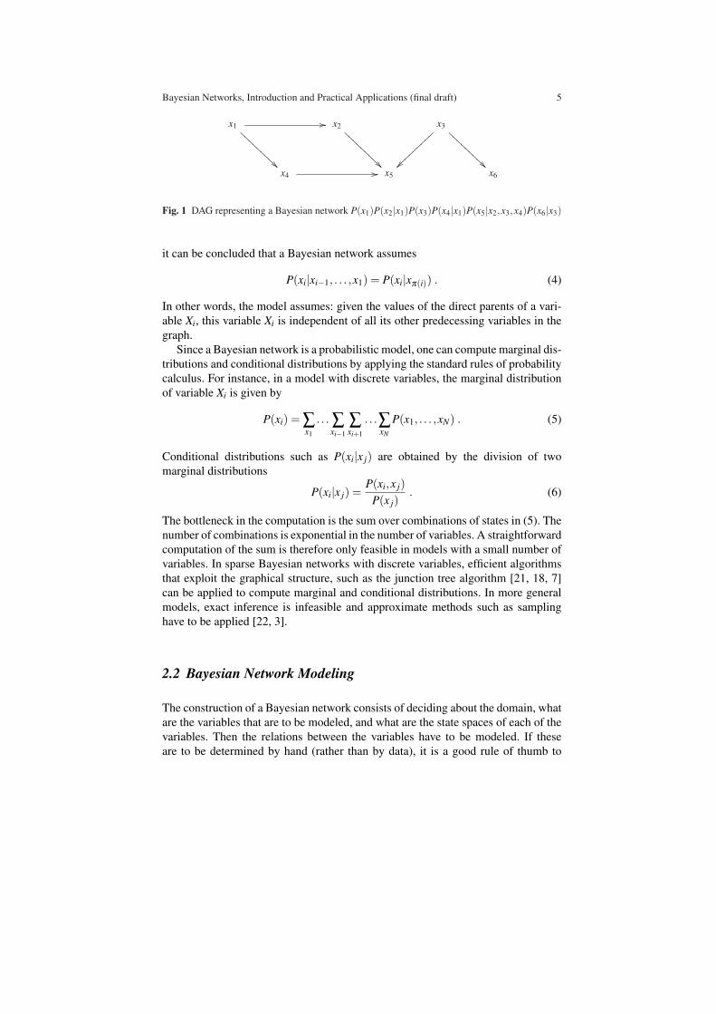
A Bayesian network is a probabilistic model P on a finite directed acyclic graph(DAG). For each node i in the graph, there is a random variable Xi together with aconditional probability distribution P(xi|xπ(i)), where π(i) are the parents of i in theDAG, see figure 1. The joint probability distribution of the Bayesian network is theproduct of the conditional probability distributions

P(x1, . . . ,xn) =n

∏i=1

P(xi|xπ(i)) . (2)

Since any DAG can be ordered such that π(i)⊆ 1, . . . i−1 and any joint distribu-tion can be written as

P(x1, . . . ,xn) =n

∏i=1

P(xi|xi−1, . . . ,x1) , (3)


x1 //

ÃÃAAA

AAAA

AAx2

ÃÃAAA

AAAA

AAx3

~~}}}}

}}}}

}

ÃÃAAA

AAAA

AA

x4 // x5 x6

Fig. 1 DAG representing a Bayesian network P(x1)P(x2|x1)P(x3)P(x4|x1)P(x5|x2,x3,x4)P(x6|x3)

it can be concluded that a Bayesian network assumes

P(xi|xi−1, . . . ,x1) = P(xi|xπ(i)) . (4)

In other words, the model assumes: given the values of the direct parents of a vari-able Xi, this variable Xi is independent of all its other predecessing variables in thegraph.

Since a Bayesian network is a probabilistic model, one can compute marginal dis-tributions and conditional distributions by applying the standard rules of probabilitycalculus. For instance, in a model with discrete variables, the marginal distributionof variable Xi is given by

P(xi) = ∑x1

. . . ∑xi−1

∑xi+1

. . .∑xN

P(x1, . . . ,xN) . (5)

Conditional distributions such as P(xi|x j) are obtained by the division of twomarginal distributions

P(xi|x j) =P(xi,x j)

P(x j). (6)

The bottleneck in the computation is the sum over combinations of states in (5). Thenumber of combinations is exponential in the number of variables. A straightforwardcomputation of the sum is therefore only feasible in models with a small number ofvariables. In sparse Bayesian networks with discrete variables, efficient algorithmsthat exploit the graphical structure, such as the junction tree algorithm [21, 18, 7]can be applied to compute marginal and conditional distributions. In more generalmodels, exact inference is infeasible and approximate methods such as samplinghave to be applied [22, 3].

2.2 Bayesian Network Modeling

The construction of a Bayesian network consists of deciding about the domain, whatare the variables that are to be modeled, and what are the state spaces of each of thevariables. Then the relations between the variables have to be modeled. If theseare to be determined by hand (rather than by data), it is a good rule of thumb to


construct a Bayesian network from cause to effect. Start with nodes that representindependent root causes, then model the nodes which they influence, and so on untilwe end at the leaves, i.e., the nodes that have no direct influence on other nodes.Such a procedure often results in sparse network structures that are understandablefor humans [27].

Sometimes this procedure fails, because it is unclear what is cause and what iseffect. Is someone’s behavior an effect of his environment, or is the environment areaction on his behavior? In such a case, just avoid the philosophical dispute, andreturn to the basics of Bayesian networks: a Bayesian network is not a model forcausal relations, but a joint probability model. The structure of the network repre-sents the conditional independence assumptions in the model and nothing else.

A related issue is the decision whether two nodes are really (conditionally) in-dependent. Usually, this is a matter of simplifying model assumptions. In the trueworld, all nodes should be connected. In practice, reasonable (approximate) assump-tions are needed to make the model simple enough to handle, but still powerfulenough for practical usage.

When the variables, states, and graphical structure is defined, the next step isto determine the conditional probabilities. This means that for each variable xi, theconditional probabilities P(xi|xπ(i)) in eqn. (4) have to be determined. In case ofa finite number of states per variable, this can be considered as a table of (|xi| −1)× |xπ(i)| entries between 0 and 1, where |xi| is the number of states of variablexi and |xπ(i)| = ∏ j∈π(i) |x j| the number of joint states of the parents. The −1 termin the (|xi|− 1) factor is due to the normalization constraint ∑xi P(xi|xπ(i)) = 1 foreach parent state. Since the number of entries is linear in the number of states of thevariables and exponential in the number of parent variables, a too large state spaceas well as a too large number of parents in the graph makes modeling practicallyinfeasible.

The entries are often just the result of educated guesses. They may be inferredfrom data, e.g. by counting frequencies of joint occurences of variables in state xiand parents in states xπ(i). For reliable estimates, however, one should have suf-ficiently many data for each joint state (xi,xπ(i)). So in this approach one shouldagain be carefull not to take state space and/or number of parents too large. A com-promise is to assume a parametrized tables. A popular choice for binary variables isthe noisy-OR table [26]. The table parametrization can be considered as an educatedguess. The parameters may then be estimated from data.

Often, models are constructed using Bayesian network software such as the ear-lier mentioned software packages. With the use of a graphical user interface (GUI),nodes can be created. Typically, nodes can assume only values from a finite set.When a node is created, it can be linked to other nodes, under the constraint thatthere are no directed loops in the network. Finally — or during this process — thetable of conditional probabilities are defined, manually or from data as mentionedabove. Many Bayesian networks that are found in literature fall into this class, seee.g., www.norsys.com/netlibrary/. In figure 2, a part of the ALARM network asrepresented in BayesBuilder (www.snn.ru.nl/) is plotted. The ALARM network wasoriginally designed as a network for monitoring patients in intensive care [2]. It con-


Fig. 2 Screen shot of part of the ’Alarm network’ in the BayesBuilder GUI

sists of 37 variables, each with 2, 3, or 4 states. It can be considered as a relativelylarge member of this class of models. An advantage of the GUI based approachis that a small or medium sized Bayesian network, i.e., with up to a few dozen ofvariables, where each variable can assume a few states, can be developed quickly,without the need of expertise on Bayesian networks modeling or inference algo-rithms.

3 An Example Application: Medical Diagnosis

In this section we will consider the a Bayesian network for medical diagnosis ofthe respiratory system. This is model is inspired on the famous ’ASIA network’described in [21].

3.1 Modeling

We start by considering the the following piece of qualitative ’knowledge’:

The symptom dyspnoea (shortness of breath) may be due to the diseases pneumonia, lungcancer, and/or bronchitis. Patients with pneumonia, and/or bronchitis often have a verynasty wet coughing. Pneumonia, and/or lung cancer are often accompanied by a heavychest pain. Pneumonia is often causing a severe fever, but this may also be caused by acommon cold. However, a common cold is often recognized by a runny nose. Sometimes,wet coughing, chest pain, and/or dyspnoea occurs unexplained, or are due to another cause,without any of these diseases being present. Sometimes diseases co-occur. A weakenedimmune-system (for instance, homeless people, or HIV infected) increases the probabilityof getting an pneumonia. Also, lung cancer increases this probability. Smoking is a seriousrisk factor for bronchitis and for lung cancer.


immun sys

²²

smoking

²² ##GGGGGGGGGGG

comm cold

{{wwww

wwww

wwww

²²

pneumonia

{{wwwwwwwwwww

²² ##GGGGGGGGGGG

))SSSSSSSSSSSSSSSSSSSSSSSSlung canceroo

{{wwwwwwwwwww

##GGGGGGGGGGGbronchitis

{{wwwwwwwwwww

²²

runny nose fever chest pain coughing dyspnoea

Fig. 3 DAG for the respiratory medicine toy model. See text for details

Now to build a model, we first have to find out which are the variables. In the textabove, these are the ones printed in italics. In a realistic medical application, onemay want to model multi-state variables. For simplicity, however, we take in thisexample all variables binary (true/false). Note that by modeling diseases as separatevariables rather than by mutually exclusive states in a single disease variable, themodel allows diseases to co-occur.

The next step is to figure out a sensible graphical structure. In the graphical repre-sentation of the model, i.e., in the DAG, all these variables are represented by nodes.The question now is which arrows to draw between the nodes. For this, we will usethe principle of causal modeling. We derive these from the ’qualitative knowledge’and some common sense. The general causal modeling assumption in this medicaldomain is that risk factors ’cause’ the diseases, so risk factors will point to diseases,and diseases ’cause’ symptoms, so diseases will point to symptoms.

We start by modeling risk factors and diseases. Risk factors are weakenedimmune-system (for pneumonia), smoking (for bronchitis and for lung cancer), andlung cancer (also for pneumonia). The nodes for weakened immune-system andsmoking have no incoming arrows, since there are no explicit causes for these vari-ables in the model. We draw arrows from these node to the diseases for which theyare risk factors. Furthermore, we have a node for the disease common cold. Thisnode has no incoming arrow, since no risk factor for this variable is modeled.

Next we model the symptoms. The symptom dyspnoea may be due to the dis-eases pneumonia, lung cancer, and/or bronchitis, so we draw an arrow from all thesediseases to dyspnoea. In a similar way, we can draw arrows from pneumonia, andbronchitis to wet coughing; arrows from pneumonia, and lung cancer to chest pain;arrows from pneumonia and common cold to fever; and an arrow from common coldto runny nose. This completes the DAG, which can be found in figure 3. (In thefigures and in some of the text in the remainder of the section we abbreviated someof the variable names, e.g. we used immun sys instrad of weakened immune-system,etc.)


P(immun syst)0.05

P(smoking)0.3

P(common cold)0.35

P(lung cancer smoking)0.1 true

0.01 false

P(bronchitis smoking)0.3 true

0.01 false

P(runny nose common cold)0.9 true0.01 false

P(pneumonia immun syst, lung cancer)0.3 true true0.3 true false0.05 false true0.001 false false

P(fever pneumonia, common cold)0.9 true true0.9 true false0.2 false true0.01 false false

P(cough pneumonia, bronchitis)0.9 true true0.9 true false0.9 false true0.1 false false

P(chest pain pneumonia, bronchitis)0.9 true true0.9 true false0.9 false true0.1 false false

P(dyspnoea bronchitis, lung cancer, pneumonia)0.8 true true true0.8 true true false0.8 true false true0.8 true false false0.5 false true true0.5 false true false0.5 false false true0.1 false false false

Fig. 4 Conditional probability tables parametrizing the respiratory medicine toy model. The num-bers in the nodes represent the marginal probabilities of the variables in state ’true’. See text fordetails

The next step is the quantitative part, i.e., the determination of the conditionalprobability tables. The numbers that we enter are rather arbitrary guesses and we donot pretend them to be anyhow realistic. In determining the conditional probabili-ties, we used some modeling assumptions such as that the probability of a symptomin the presence of an additional causing diseases is at least as high as the proba-bility of that symptom in the absence of that disease. The tables as presented infigure 4. In these tables, the left column represents the probability values in the truestate, P(variablename) ≡ P(variablename = true), so P(variablename = false) =1−P(variablename). The other columns indicate the joint states of the parent vari-ables.

3.2 Reasoning

Now that the model is defined, we can use it for reasoning, e.g. by entering obser-vational evidence into the system and doing inference, i.e. computing conditionalprobabilities given this evidence. To do the computation, we have modeled the sys-tem in BayesBuilder. In figure 5 we show a screen shot of the Bayesian network asmodeled in BayesBuilder. The program uses the junction tree inference algorithm tocompute the marginal node probabilities and displays them on screen. The marginal


Fig. 5 Screen shot of the respiratory medicine toy model in the BayesBuilder GUI. Red barspresent marginal node probabilities

node probabilities are the probability distributions of each of the variables in theabsence of any additional evidence. In the program, evidence can be entered byclicking on a state of the variable. This procedure is sometimes called ‘clamping’.The node probabilities will then be conditioned on the clamped evidence. With this,we can easily explore how the models reasons.

3.2.1 Knowledge representation

Bayesian networks may serve as a rich knowledge base. This is illustrated by con-sidering a number of hypothetical medical guidelines and comparing these withBayesian network inference results. These results will also serve to comment onsome of the typical behavior in Bayesian networks.

1. In case of high fever in absence of a runny nose, one should consider pneumonia.

Inference We clamp fever = true and runny nose = false and look at the con-ditional probabilities of the four diseases. We see that in particular the proba-bility of pneumonia is increased from about 2% to 45%. See figure 6.

Comment There are two causes in the model for fever, namely has parentspneumonia and common cold. However, the absence of acommon cold makescommon cold less likely. This makes the other explaining cause pneumoniamore likely.

2. Lung cancer is often found in patients with chest pain, dyspnoea, no fever, andusually no wet coughing.


Fig. 6 Model in the state representing medical guideline 1, see main text. Red bars present condi-tional node probabilities, conditioned on the evidence (bleu bars)

Inference We clamp chest pain = true, dyspnoea = true, fever = false, andcoughing = false We see that probability of lung cancer is raised 0.57. Evenif we set coughing = true, the probability is still as high as 0.47.

Comment Chest pain and dyspnoea can both be caused by lung cancer. How-ever, chest pain for example, can also be caused by pneumonia. The absenceof in particular fever makes pneumonia less likely and therefore lung cancermore likely. To a lesser extend this holds for absence of coughing and bron-chitis.

3. Bronchitis and lung cancer are often accompanied, e.g patients with bronchi-tis often develop a lung cancer or vice versa. However, these diseases have noknown causal relation, i.e., bronchitis is not a cause of lung cancer, and lungcancer is not a cause of bronchitis.

Inference According to the model, P(lung cancer|bronchitis = true) = 0.09and P(bronchitis|lung cancer = true) = 0.25. Both probabilities are more thantwice the marginal probabilities (see figure 3).

Comment Both diseases have the same common cause: smoking. If the state ofsmoking is observed, the correlation is broken.

3.2.2 Diagnostic reasoning

We can apply the system for diagnosis. the idea is to enter the patient observa-tions, i.e. symptoms and risk factors into the system. Then diagnosis (i.e. findingthe cause(s) of the symptoms) is done by Bayesian inference. In the following, we


present some hypothetical cases, present the inference results and comment on thereasoning by the network.

1. Mr. Appelflap calls. He lives with his wife and two children in a nice little housein the suburb. You know him well and you have good reasons to assume that hehas no risk of a weakened immune system. Mr. Appelflap complains about highfever and a nasty wet cough (although he is a non-smoker). In addition, he soundsrather nasal. What is the diagnosis?

Inference We clamp the risk factors immun sys = false, smoking = false andthe symptoms fever = true, runny nose = true. We find all disease probabili-ties very small, except common cold, which is almost certainly true.

Comment Due to the absence of risk factors, the prior probabilities of theother diseases that could explain the symptoms is very small compared tothe prior probability of common cold. Since common cold also explains allthe symptoms, that disease takes all the probability of the other causes. Thisphenomenon is called ’explaining away’: pattern of reasoning in which theconfirmation of one cause (common cold, with a high prior probability andconfirmed by runny nose ) of an observed event (fever) reduces the need toinvoke alternative causes (pneumonia as an explanation of fever).

2. The salvation army calls. An unknown person (looking not very well) has arrivedin their shelter for homeless people. This person has high fever, a nasty wet cough(and a runny nose.) What is the diagnosis?

Inference We suspect a weakened immune system, so the system we clampthe risk factor immun sys = true. As in the previous case, the symptoms arefever = true,mboxrunnynose = true. However, now we not only find common cold with ahigh probability (P = 0.98), but also pneumonia (P = 0.91).

Comment Due to the fact that with a weakened immune system, the prior prob-ability of pneumonia is almost as high as the prior probability of commoncold. Therefore the conclusion is very different from the previous cas. Notethat for this diagnosis, it is important that diseases can co-occur in the model.

3. A patient suffers from a recurrent pneumonia. This patient is a heavy smoker butotherwise leads a ‘normal’, healthy live, so you may assume there is no risk of aweakened immune system. What is your advice?

Inference We clamp immun sys = false, smoking = true, and pneumonia =true. As a result, we see that there is a high probability of lung cancer.

Comment The reason is that due to smoking, the prior of disease is increased.More importantly, however, is that weakened immune system is excluded ascause of the pneumonia, so that lung cancer remains as the most likely expla-nation of the cause of the recurrent pneumonia.


Fig. 7 Diagnosing mr. Appelflap. Primary diagnosis: common cold. See main text

Fig. 8 Salvation army case. Primary diagnosis: pneumonia. See main text

3.3 Discussion

With the toy model, we aimed to illustrate the basic principles of Bayesian net-work modeling. With the inference examples, we have aimed to demonstrate someof typical reasoning capabilities of Bayesian networks. One features of Bayesiannetworks that distinguish them from e.g. conventional feedforward neural networksis that reasoning is in arbitrary direction, and with arbitrary evidence. Missing dataor observations are dealt with in a natural way by probabilistic inference. In manyapplications, as well as in the examples in this section, the inference question isto compute conditional node probabilities. These are not the only quantities thatone could compute in a Bayesian networks. Other examples are are correlations be-


Fig. 9 Recurrent pneumonia case. Primary diagnosis: lung cancer. See main text

tween variables, the probability of the joint state of the the nodes, or the entropy of aconditional distribution. Applications of the latter two will be discussed in the nextsections.

In the next sections we will discuss two Bayesian networks for real world appli-cations The modeling principles are basically the same as in the toy model describedin this section. There are some differences, however. In the first model, the networkconsists of a few types of nodes that have simple and well defined relations amongeach other. However, for each different case in the application, a different networkhas to be generated. It does not make sense for this application to try to build thesenetworks beforehand in a GUI. In the second one the complexity is more in the vari-ables themselves than in the network structure. Dedicated software has been writtenfor both modeling and inference.

4 Bonaparte: a Bayesian Network for Disaster VictimIdentification

Society is increasingly aware of the possibility of a mass disaster. Recent examplesare the WTC attacks, the tsunami, and various airplane crashes. In such an event, therecovery and identification of the remains of the victims is of great importance, bothfor humanitarian as well as legal reasons. Disaster victim identification (DVI), i.e.,the identification of victims of a mass disaster, is greatly facilitated by the adventof modern DNA technology. In forensic laboratories, DNA profiles can be recordedfrom small samples of body remains which may otherwise be unidentifiable. Theidentification task is the match of the unidentified victim with a reported missingperson. This is often complicated by the fact that the match has to be made in anindirect way. This is the case when there is no reliable reference material of the


missing person. In such a case, DNA profiles can be taken from relatives. Sincetheir profiles are statistically related to the profile of the missing person (first degreefamily members share about 50% of their DNA) an indirect match can be made.

In cases with one victim, identification is a reasonable straightforward task forforensic researchers. In the case of a few victims, the puzzle to match the victimsand the missing persons is often still doable by hand, using a spread sheet, or withsoftware tools available on the internet [10]. However, large scale DVI is infeasiblein this way and an automated routine is almost indispensable for forensic institutesthat need to be prepared for DVI.

?

?

?

?

Fig. 10 The matching problem. Match the unidentified victims (blue, right) with reported missingpersons (red, left) based on DNA profiles of victims and relatives of missing persons. DNA profilesare available from individuals represented by solid squares (males) and circles (females).

Bayesian networks are very well suited to model the statistical relations of ge-netic material of relatives in a pedigree [12]. They can directly be applied in kinshipanalysis with any type of pedigree of relatives of the missing persons. An additionaladvantage of a Bayesian network approach is that it makes the analysis tool moretransparent and flexible, allowing to incorporate other factors that play a role —such as measurement error probability, missing data, statistics of more advancedgenetic markers etc.

Recently, we have developed software for DVI, called Bonaparte. This devel-opment is in collaboration with NFI (Netherlands Forensic Institute). The compu-tational engine of Bonaparte uses automatically generated Bayesian networks andBayesian inference methods, enabling to correctly do kinship analysis on the basisof DNA profiles combined with pedigree information. It is designed to handle largescale events, with hundreds of victims and missing persons. In addition, it has graph-ical user interface, including a pedigree editor, for forensic analysts. Data-interfacesto other laboratory systems (e.g., for the DNA-data input) will also be implemented.


In the remainder of this section we will describe the Bayesian model approachthat has been taken in the development of the application. We formulate the com-putational task, which is the computation of the likelihood ratio of two hypotheses.The main ingredient is a probabilistic model P of DNA profiles. Before discussingthe model, we will first provide a brief introduction to DNA profiles. In the last partof the section we describe how P is modeled as a Bayesian network, and how thelikelihood ratio is computed.

4.1 Likelihood Ratio of Two Hypotheses

Assume we have a pedigree with an individual MP who is missing (the MissingPerson). In this pedigree, there are some family members that have provided DNAmaterial, yielding the profiles. Furthermore there is an Unidentified Individual UI,whose DNA is also profiled. The question is, is UI = MP? To proceed, we assumethat we have a probabilistic model P for DNA evidence of family members in apedigree. To compute the probability of this event, we need hypotheses to compare.The common choice is to formulate two hypotheses. The first is the hypothesis H1that indeed UI = MP. The alternative hypothesis H0 is that UI is an unrelated personU . In both hypotheses we have two pedigrees: the first pedigree has MP and familymembers FAM as members. The second one has only U as member. To comparethe hypotheses, we compute the likelihoods of the evidence from the DNA profilesunder the two hypotheses,

• Under Hp, we assume that MP = UI. In this case, MP is observed and U isunobserved. The evidence is E = {DNAMP +DNAFAM}.

• Under Hd , we assume that U = UI. In this case, U is observed and MP is ob-served. The evidence is E = {DNAU +DNAFAM}.

Under the model P, the likelihood ratio of the two hypotheses is

LR =P(E|Hp)P(E|Hd)

. (7)

If in addition a prior odds P(Hp)/P(Hd) is given, the posterior odds P(Hp|E)/P(Hd |E)follows directly from multiplication of the prior odds and likelihood ratio,

P(Hp|E)P(Hd |E)

=P(E|Hp)P(Hp)P(E|Hd)P(Hd)

. (8)

4.2 DNA Profiles

In this subsection we provide a brief introduction on DNA profiles for kinship analy-sis. A comprehensive treatise can be found in e.g. [6]. In humans, DNA found in the


nucleus of the cell is packed on chromosomes. A normal human cell has 46 chro-mosomes, which can be organized in 23 pairs. From each pair of chromosomes,one copy is inherited from father and the other copy is inherited from mother. In22 pairs, chromosomes are homologous, i.e., they have practically the same lengthand contain in general the same genes ( functional functional elements of DNA).These are called the autosomal chromosomes. The remaining chromosome is thesex-chromosome. Males have an X and a Y chromosome. Females have two X chro-mosomes.

More than 99% of the DNA of any two humans of the general population isidentical. Most DNA is therefore not useful for identification. However, there arewell specified locations on chromosomes where there is variation in DNA amongindividuals. Such a variation is called a genetic marker. In genetics, the specifiedlocations are called loci. A single location is a locus.

In forensic research, the short tandem repeat (STR) markers are currently mostused. The reason is that they can be reliable determined from small amounts of bodytissue. Another advantage is that they have a low mutation rate, which is importantfor kinship analysis. STR markers is a class of variations that occur when a patternof two or more nucleotides is repeated. For example,

(CAT G)3 = CAT GCAT GCAT G . (9)

The number of repeats x (which is 3 in the example) is the variation among thepopulation. Sometimes, there is a fractional repeat, e.g. CAT GCAT GCAT GCA, thiswould be encoded with repeat number x = 3.2, since there are three repeats andtwo additional nucleotides. The possible values of x and their frequencies are welldocumented for the loci used in forensic research. These ranges and frequenciesvary between loci. To some extend they vary among subpopulations of humans. TheSTR loci are standardized. The NFI uses CODIS (Combined DNA Index System)standard with 13 specific core STR loci, each on different autosomal chromosomes.

The collection of markers yields the DNA profile. Since chromosomes exist inpairs, a profile will consist of pairs of markers. For example in the CODIS standard,a full DNA profile will consist of 13 pairs (the following notation is not commonstandard)

x = (1x1,1x2),(2x1,2x2), . . . ,(13x1,13x2) , (10)

in which each µxs is a number of repeats at a well defined locus µ . However, sincechromosomes exists in pairs, there will be two alleles µx1 and µx2 for each location,one paternal — on the chromosome inherited from father — and one maternal. Un-fortunately, current DNA analysis methods cannot identify the phase of the alleles,i.e., whether an allele is paternal or maternal. This means that (µx1,µ x2) cannot bedistinguished from (µx2,µ x1). In order to make the notation unique, we order theobserved alleles of a locus such that µx1 ≤ µx2.

Chromosomes are inherited from parents. Each parent passes one copy of eachpair of chromosomes to the child. For autosomal chromosomes there is no (known)preference which one is transmitted to the child. There is also no (known) correla-tion between the transmission of chromosomes from different pairs. Since chromo-


j k

j

x j xpj

ww

''NNNNNNNNNNNNNNNNN xmj

ww

ÁÁ>>>

>>>>

>>xp

k

¡¡¡¡¡¡

¡¡¡¡

¡

''xm

k

wwpppppppppppppppp((

xk

xi xpihh xm

ihh

Fig. 11 A basic pedigree with father, mother, and child. Squares represent males, circles representfemales. Right: corresponding Bayesian network. Grey nodes are observables. xp

j and xmj represents

paternal and maternal allele of individual j. See text.

somes are inherited from parents, alleles are inherited from parents as well. How-ever, there is a small probability that an allele is changed or mutated. This mutationprobability is about 0.1%.

Finally in the DNA analysis, sometimes failures occur in the DNA analysismethod and an allele at a certain locus drops out. In such a case the observationis (µx1,F), in which “F” is a wild card.

4.3 A Bayesian Network for Kinship Analysis

In this subsection we will describe the building blocks of a Bayesian network tomodel probabilities of DNA profiles of individuals in a pedigree. First we observethat inheritance and observation of alleles at different loci are independent. So foreach locus we can make an independent model Pµ . In the model description below,we will consider a model for a single locus, and we will suppress the µ dependencyfor notational convenience.

4.3.1 Allele Probabilities

We will consider pedigrees with individuals i. In a pedigree, each individual i hastwo parents, a father f (i) and a mother m(i). An exception is when a individual is afounder. In that case it has no parents in the pedigree.

Statistical relations between DNA profiles and alleles of family members can beconstructed from the pedigree, combined with models for allele transmission . Onthe given locus, each individual i has a paternal allele x f

i and an maternal allele xmi . f

and m stands for ‘father’ and ‘mother’. The pair of alleles is denoted as xi = (x fi ,xm

i ).Sometimes we use superscript s which can have values { f ,m}. So each allele in thepedigree is indexed by (i,s), where i runs over individuals and s over phases ( f ,m).The alleles can assume N values, where N as well as the allele values depend on thelocus.

An allele from a founder is called ‘founder allele’. So a founder in the pedigreehas two founder alleles. The simplest model for founder alleles is to assume thatthey are independent, and each follow a distribution P(a) of population frequencies.


This distribution is assumed to be given. In general P(a) will depend on the locus.More advanced models have been proposed in which founder alleles are correlated.For instance, one could assume that founders in a pedigree come from a singlebut unknown subpopulation [1]. This model assumption yield corrections to theoutcomes in models without correlations between founders. A drawback is that thesemodels may lead to a severe increase in required memory and computation time. Inthis chapter we will restrict ourself to models with independent founder alleles.

If an individual i has its parents in the pedigree the allele distribution of an indi-vidual given the alleles of its parents are as follows,

P(xi|x f (i),xm(i)) = P(x fi |x f (i))P(xm

i |xm(i)) , (11)

where

P(x fi |x f (i)) =

12 ∑

s= f ,mP(x f

i |xsf (i)) , (12)

P(xmi |xm(i)) =

12 ∑

s= f ,mP(xm

i |xsm(i)) . (13)

To explain (12) in words: individual i obtains its paternal allele x fi from its father

f (i). However, there is a 50% chance that this allele is the paternal allele x ff (i) of

father f (i) and a 50% chance that it is his maternal allele xmf (i). A similar explanation

applies to (13).The probabilities P(x f

i |xsf (i)) and P(xm

i |xsm(i)) are given by a mutation model

P(a|b), which encodes the probability that allele of the child is a while the alleleon the parental chromosome that is transmitted is b. The precise mutation mecha-nisms for the different STR markers are not known. There is evidence that muta-tions from father to child are in general about 10 times as probable as mutationsfrom mother to child. Gender of each individual is assumed to be known, but fornotational convenience we suppress dependency of parent gender. In general, muta-tion tends to decrease with the difference in repeat numbers |a−b|. Mutation is alsolocus dependent [4].

Several mutation models have been proposed, see e.g. [8]. As we will see later,however, the inclusion of a detailed mutation model may lead to a severe increasein required memory and computation time. Since mutations are very rare, one couldask if there is any practical relevance in a detailed mutation model. The simplestmutation model is of course to assume the absence of mutations, P(a|b) = δa,b.Such model enhances efficient inference. However, any mutation in any single locuswould lead to a 100% rejection of the match, even if there is a 100% match in theremaining markers. Mutation models are important to get some model toleranceagainst such case. The simplest non-trivial mutation model is a uniform mutationmodel with mutation rate µ (not to be confused with the locus index µ),


P(a|a) = 1−µ , (14)P(a|b) = µ/(N−1) if a 6= b . (15)

Mutation rate may depend on locus and gender.An advantage of this model is that the required memory and computation time

increases only slightly compared to the mutation free model. Note that the popu-lation frequency is in general not invariant under this model: the mutation makesthe frequency more flat. One could argue that this is a realistic property that intro-duces diversity in the population. In practical applications in the model, however,the same population frequency is assumed to apply to founders in different genera-tions in a pedigree. This implies that if more unobserved references are included inthe pedigree to model ancestors of an individual, the likelihood ratio will (slightly)change. In other words, formally equivalent pedigrees will give (slightly) differentlikelihood ratios.

4.3.2 Observations

Observations are denoted as xi, or x if we do not refer to an individual. The parentalorigin of an allele can not be observed, so alleles x f = a,xm = b yields the sameobservation as x f = b,xm = a. We adopt the convention to write the smallest allelefirst in the observation: x = (a,b) ⇔ a ≤ b. In the case of an allele loss, we writex = (x,F) where F stands for a wild card. We assume that the event of an allele losscan be observed (e.g. via the peak hight [6]). This event is modeled by L. With L = 1there is allele loss, and there will be a wild card ?. A full observation is coded asL = 0. The case of loss of two alleles is not modeled, since in that case we simplyhave no observation.

The observation model is now straightforwardly written down. Without alleleloss (L = 0), alleles y results in an observation y. This is modeled by the determin-istic table

P(x|y,L = 0) ={

1 if x = y ,0 otherwise. (16)

Note that for a given y there is only one x with x = y.With allele loss (L = 1), we have

P(x = (a,F)|(a,b),L = 1) = 1/2 if a 6= b (17)P(x = (b,F)|(a,b),L = 1) = 1/2 if a 6= b (18)P(x = (a,F)|(a,a),L = 1) = 1 . (19)

I.e., if one allele is lost, the alleles (a,b) leads to an observation a (then b is lost),or to an observation b (then a is lost). Both events have 50% probability. If bothalleles are the same, so the pair is (a,a), then of course a is observed with 100%probability.


4.4 Inference

By multiplying all allele priors, transmission probabilities and observation models, aBayesian network of alleles x and DNA profiles of individuals x in a given pedigreeis obtained. Assume that the pedigree consists of a set of individuals I = 1, . . . ,Kwith a subset of founders F, and assume that allele losses L j are given, then thisprobability reads

P({x,x}I) = ∏j

P(x j|x j,L j) ∏i∈I\F

P(xi|x f (i),xm(i))∏i∈F

P(xi) . (20)

Under this model the likelihood of a given set DNA profiles can now be com-puted. If we have observations x j from a subset of individuals j ∈ O, the likelihoodof the observations in this pedigree is the marginal distribution P({x}O), which isthe marginal probability

P({x}O) = ∑x1

. . .∑xK

∏j∈O

P(x j|x j,L j) ∏i∈I\F

P(xi|x f (i),xm(i))∏i∈F

P(xi) . (21)

This computation involves the sum over all states of allele pairs xi of all individuals.In general, the allele-state space can be prohibitively large. This would make even

the junction tree algorithm infeasible if it would straightforwardly be applied. For-tunately, a significant reduction in memory requirement can be achieved by “valueabstraction”: if the observed alleles in the pedigree are all in a subset A of M dif-ferent allele values, we can abstract from all unobserved allele values and considerthem as a single state z. If an allele is z, it means that it has a value that is not in theset of observed values A. We now have a system in which states can assume onlyM +1 values which is generally a lot smaller than N, the number of a priori possibleallele values. This procedure is called value abstraction [14]. The procedure is ap-plicable if for any a ∈ A, L ∈ {0,1}, and b1,b2,b3,b4 6∈ A, the following equalitieshold

P(a|b1) = P(a|b2) (22)P(x|a,b1,L) = P(x|a,b2,L) (23)P(x|b1,a,L) = P(x|b2,a,L) (24)

P(x|b1,b2,L) = P(x|b3,b4,L) (25)

If these equalities hold, then we can replace P(a|b) by P(a|z) and P(x|a,b) byP(x|a,z) etc. in the abstracted state representation. The conditional probability ofz then follows from

P(z|x) = 1− ∑a∈A

P(a|x) (26)

for all x in A∪ z. One can also easily check that the observation probabilities satisfythe condition. The uniform mutation model satisfies condition (22) since P(a|b) =


+

XML Web browserhttps

Report Generation

Computationalcore

AdministrationData import

Web browserhttpsExcel Internal

database

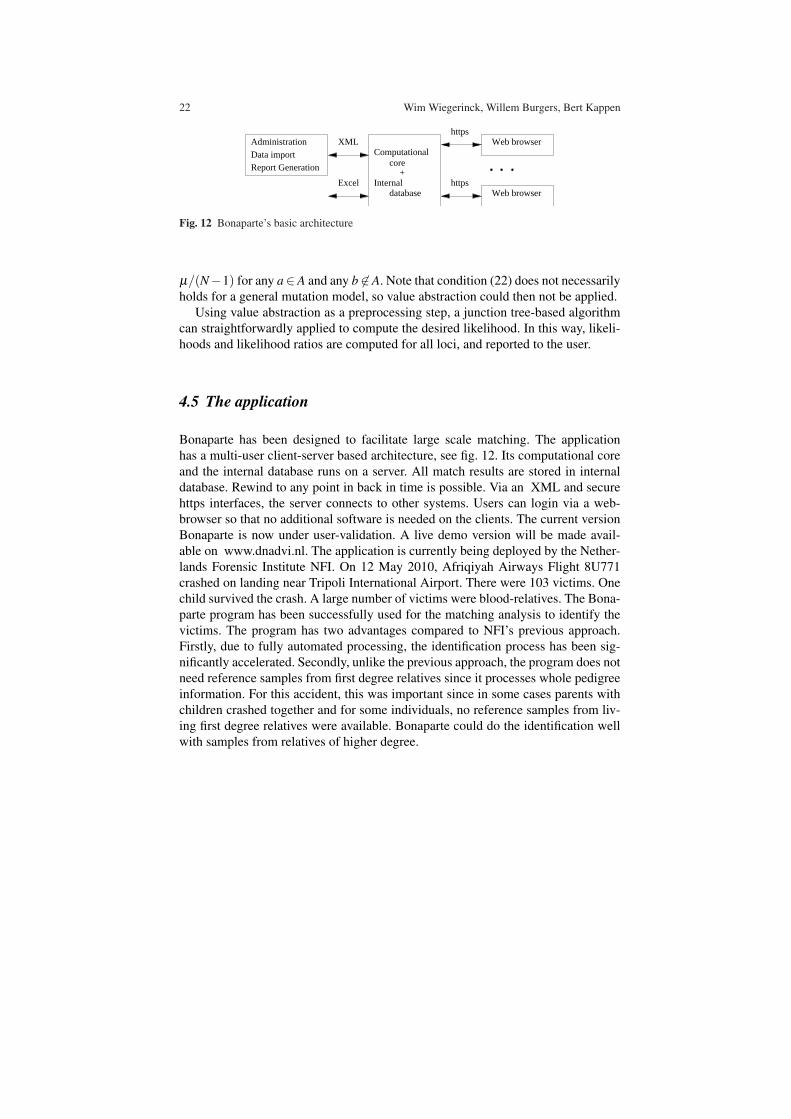
Fig. 12 Bonaparte’s basic architecture

µ/(N−1) for any a∈A and any b 6∈A. Note that condition (22) does not necessarilyholds for a general mutation model, so value abstraction could then not be applied.

Using value abstraction as a preprocessing step, a junction tree-based algorithmcan straightforwardly applied to compute the desired likelihood. In this way, likeli-hoods and likelihood ratios are computed for all loci, and reported to the user.

4.5 The application

Bonaparte has been designed to facilitate large scale matching. The applicationhas a multi-user client-server based architecture, see fig. 12. Its computational coreand the internal database runs on a server. All match results are stored in internaldatabase. Rewind to any point in back in time is possible. Via an XML and securehttps interfaces, the server connects to other systems. Users can login via a web-browser so that no additional software is needed on the clients. The current versionBonaparte is now under user-validation. A live demo version will be made avail-able on www.dnadvi.nl. The application is currently being deployed by the Nether-lands Forensic Institute NFI. On 12 May 2010, Afriqiyah Airways Flight 8U771crashed on landing near Tripoli International Airport. There were 103 victims. Onechild survived the crash. A large number of victims were blood-relatives. The Bona-parte program has been successfully used for the matching analysis to identify thevictims. The program has two advantages compared to NFI’s previous approach.Firstly, due to fully automated processing, the identification process has been sig-nificantly accelerated. Secondly, unlike the previous approach, the program does notneed reference samples from first degree relatives since it processes whole pedigreeinformation. For this accident, this was important since in some cases parents withchildren crashed together and for some individuals, no reference samples from liv-ing first degree relatives were available. Bonaparte could do the identification wellwith samples from relatives of higher degree.


4.6 Summary

Bonaparte is an application of Bayesian networks for victim identification by kin-ship analysis based on DNA profiles. The Bayesian networks are used to modelstatistical relations between DNA profiles of different individuals in a pedigree. ByBayesian inference, likelihood ratios and posterior odds of hypotheses are com-puted, which are the quantities of interest for the forensic researcher. The probabilis-tic relations between variables are based on first principles of genetics. A feature ofthis application is the automatic, on-the-fly derivation of models from data, i.e., thepedigree structure of a family of a missing person. The approach is related to theidea of modeling with templates, which is discussed in e.g. [20].

5 A Petrophysical Decision Support System

Oil and gas reservoirs are located in the earth’s crust at depths of several kilometers,and when located offshore, in water depths of a few meters to a few kilometers.Consequently, the gathering of critical information such as the presence and type ofhydrocarbons, size of the reservoir and the physical properties of the reservoir suchas the porosity of the rock and the permeability is a key activity in the oil and gasindustry.

Pre-development methods to gather information on the nature of the reservoirsrange from gravimetric, 2D and 3D seismic to the drilling of exploration and ap-praisal boreholes. Additional information is obtained while a field is developedthrough data acquisition in new development wells drilled to produce hydrocarbons,time-lapse seismic surveys and in-well monitoring of how the actual production ofhydrocarbons affects physical properties such as the pressure and temperature. Thepurpose of information gathering is to decide which reservoirs can be developedeconomically, and how to adapt the means of development best to the particularnature of a reservoir.

The early measurements acquired in exploration, appraisal and developmentboreholes are a crucial component of the information gathering process. These mea-surements are typically obtained from tools on the end of a wireline that are loweredinto the borehole to measure the rock and fluid properties of the formation. Their isa vast range of possible measurement tools [28]. Some options are very expensiveand may even risk other data acquisition options. In general acquiring all possibledata imposes too great an economic burden on the exploration, appraisal and devel-opment. Hence data acquisition options must be exercised carefully bearing in mindthe learnings of already acquired data and general hydrocarbon field knowledge.Also important is a clear understanding of what data can and cannot be acquiredlater and the consequences of having an incorrect understanding of the nature of areservoir on the effectiveness of its development.

Making the right data acquisition decisions, as well as the best interpretation ofinformation obtained in boreholes forms one of the principle tasks of petrophysi-


cists. The efficiency of a petrophysicist executing her/his task is substantially in-fluenced by the ability to gauge her/his experience to the issues at hand. Efficiencyis hampered when a petrophysicists experience level is not yet fully sufficient andby the rather common circumstance that decisions to acquire particular types of in-formation or not must be made in a rush, at high costs and shortly after receivingother information that impact on that very same decision. Mistakes are not entirelyuncommon and almost always painful. In some cases, non essential data is obtainedat the expense of extremely high cost, or essential data is not obtained at all; causingdevelopment mistakes that can jeopardize the amount of hydrocarbon recoverablefrom a reservoir and induce significant cost increases.

The overall effectiveness of petrophysicists is expected to improve using a de-cision support system (DSS). In practice a DSS can increase the petrophysicists’awareness of low probability but high impact cases and alleviate some of the oper-ational decision pressure.

In cooperation with Shell E&P, SNN has developed a DSS tool based on aBayesian network and an efficient sampler for inference. The main tasks of the ap-plication is the estimation of compositional volume fractions in a reservoir on thebasis of measurement data. In addition it provides insight in the effect of additionalmeasurements. Besides an implementation of the model and the inference, the toolcontains graphical user interface in which the user can take different views on thesampled probability distribution and on the effect of additional measurements.

In the remainder of this section, we will describe the Bayesian network approachfor the DSS tool. We focus on our modeling and inference approach. More detailsare described in the full paper [5].

5.1 Probabilistic modeling

The primary aim of the model is to estimate the compositional volume fractions ofa reservoir on the basis of borehole measurements. Due to incomplete knowledge,limited amount of measurements, and noise in the measurements, there will be un-certainty in the volume fractions. We will use Bayesian inference to deal with thisuncertainty.

The starting point is a model for the probability distribution P(v,m) of the com-positional volume fractions v and borehole measurements m. A causal argument“The composition is given by the (unknown) volume fractions, and the volume frac-tions determine the distribution measurement outcomes of each of the tools” leadsus to a Bayesian network formulation of the probabilistic model,

P(v,m) =Z

∏i=1

P(mi|v)P(v) . (27)

In this model, P(v) is the so-called prior, the prior probability distribution of volumefractions before having seen any data. In principle, the prior encodes the generic ge-


ological and petrophysical knowledge and beliefs [30]. The factor ∏Zi=1 P(mi|v) is

the observation model. The observation model relates volume fractions v to mea-surement outcomes mi of each of the Z tools i. The observation model assumes thatgiven the underlying volume fractions, measurement outcomes of the different toolsare independent. Each term in the observation model gives the probability densityof observing outcome mi for tool i given that the composition is v. Now given a setof measurement outcomes mo of a subset Obs of tools, the probability distributionof the volume fractions can be updated in a principled way by applying Bayes’ rule,

P(v|mo) =∏i∈Obs P(mo

i |v)P(v)P(mo)

. (28)

The updated distribution is called the posterior distribution. The constant in thedenominator P(mo) =

∫v ∏i∈Obs P(mo

i |v)P(v)dv is called the evidence.In our model, v is a 13 dimensional vector. Each component represents the vol-

ume fraction of one of 13 most common minerals and fluids (water, calcite, quartz,oil, etc.). So each component is bounded between zero and one. The componentssum up to one. In other words, the volume fractions are confined to a simplexSK = {v|0 ≤ v j ≤ 1,∑k vk = 1}. There are some additional physical constraints onthe distribution of v, for instance that the total amount of fluids should not exceed40% of the total formation. The presence of more fluids would cause a collapse ofthe formation.

Each tool measurement gives a one-dimensional continuous value. The relationbetween composition and measurement outcome is well understood. Based on thephysics of the tools, petrophysicists have expressed these relations in terms of deter-ministic functions f j(v) that provide the idealized noiseless measurement outcomesof tool j given the composition v [30]. In general, the functions f j are nonlinear.For most tools, the noise process is also reasonably well understood — and can bedescribed by either a Gaussian (additive noise) or a log-Gaussian (multiplicativenoise) distribution.

A straightforward approach to model a Bayesian network would be to discretizethe variables and create conditional probability tables for priors and conditional dis-tributions. However, due to the dimensionality of the volume fraction vector, anyreasonable discretization would result in an infeasible large state space of this vari-able. We therefore decided to remain in the continuous domain.

The remainder of this section describes the prior and observation model, as wellas the approximate inference method to obtain the posterior.

5.2 The prior and the observation model

The model has two ingredients: the prior of the volume fractions P(v) and the ob-servation model P(m j|v).


There is not much detailed domain knowledge available about the prior distri-bution. Therefore we decided to model the prior using conveniently parametrizedfamily of distributions. In our case, v ∈ SK , this lead to the Dirichlet distribution[22, 3]

Dir(v|α,µ) ∝K

∏j=1

vαµ j−1j δ

(1−

K

∑i=1

vi

). (29)

The two parameters α ∈R+ (precision) and µ ∈ SK (vector of means) can be used tofine-tune the prior to our liking. The delta function — which ensures that the simplexconstraint holds — is put here for clarity, but is in fact redundant if the model isconstraint to v ∈ SK . Additional information, e.g. the fact that the amount of fluidsmay not exceed 40% of the volume fraction can be incorporated by multiplying theprior by a likelihood term Φ(v) expressing this fact. The resulting prior is of theform

P(v) ∝ Φ(v)Dir(v|α,µ) . (30)

The other ingredient in the Bayesian network are the observation models. Formost tools, the noise process is reasonably well understood and can be reasonablywell described by either a Gaussian (additive noise) or a log-Gaussian (multiplica-tive noise) distribution. In the model, measurements are modeled as a deterministictool function plus noise,

m j = f j(v)+ξ j , (31)

in which the functions f j are the deterministic tool functions provided by domainexperts. For tools where the noise is multiplicative, a log transform is applied to thetool functions f j and the measurement outcomes m j. A detailed description of thesefunctions is beyond the scope of this paper. The noises ξ j are Gaussian and have atool specific variance σ2

j . These variances have been provided by domain experts.So, the observational probability models can be written as

P(mi|v) ∝ exp

(− (m j− f j(v))2

2σ2j

). (32)

5.3 Bayesian Inference

The next step is given a set of observations {moi }, i ∈ Obs, to compute the posterior

distribution. If we were able to find an expression for the evidence term, i.e., for themarginal distribution of the observations P(mo) =

∫v ∏i∈Obs P(mo

i |v)P(v)dv thenthe posterior distribution (28) could be written in closed form and readily evaluated.Unfortunately P(mo) is intractable and a closed-form expression does not exist. Inorder to obtain the desired compositional estimates we therefore have to resort toapproximate inference methods. Pilot studies indicated that sampling methods gavethe best performance.


The goal of any sampling procedure is to obtain a set of N samples {xi} thatcome from a given (but maybe intractable) distribution π . Using these samples wecan approximate expectation values 〈A〉 of a function A(x) according to

〈A〉=∫

xA(x)π(x)dx≈ 1

N

N

∑i=1

A(xi) . (33)

For instance, if we take A(x) = x, the approximation of the mean 〈x〉 is the samplemean 1

N ∑Ni=1 xi.

An important class of sampling methods are the so-called Markov Chain MonteCarlo (MCMC) methods [22, 3]. In MCMC sampling a Markov chain is definedthat has an equilibrium distribution π , in such a way that (33) gives a good approx-imation when applied to a sufficiently long chain x1,x2, . . . ,xN . To make the chainindependent of the initial state x0, a burn-in period is often taken into account. Thismeans that one ignores the first M ¿ N samples that come from intermediate distri-butions and begins storing the samples once the system has reached the equilibriumdistribution π .

In our application we use the hybrid Monte Carlo (HMC) sampling algorithm[11, 22]. HMC is a powerful class of MCMC methods that are designed for prob-lems with continuous state spaces, such as we consider in this section. HMC canin principle be applied to any noise model with a continuous probability density, sothere is no restriction to Gaussian noise models. HMC uses Hamiltonian dynam-ics in combination with a Metropolis [23] acceptance procedure to find regions ofhigher probability. This leads to a more efficient sampler than a sampler that relieson random walk for phase space exploration. HMC also tends to mix more rapidlythan the standard Metropolis Hastings algorithm. For details of the algorithm werefer to the literature [11, 22].

In our case, π(v) is the posterior distribution p(v|moi ) in (28). The HMC sam-

pler generates samples v1,v2, . . . ,vN from this posterior distribution. Each of the Nsamples is a full K-dimensional vector of volume fractions constraint on SK . Thenumber of samples is of the order of N = 105, which takes a few seconds on astandard PC. Figure 13 shows an example of a chain of 10 000 states generatedby the sampler. For visual clarity, only two components of the vectors are plotted(quartz and dolomite). The plot illustrates the multivariate character of the method:for example, the traces shows that the volume fractions of the two minerals tend tobe mutually exclusive: either 20% quartz, or 20% dolomite but generally not both.From the traces, all kind of statistics can be derived. As an example, the resultingone dimensional marginal distributions of the mineral volume fractions are plotted.

The performance of the method relies heavily on the quality of the sampler.Therefore we looked at the ability of the system to estimate the composition of a(synthetic) reservoir and the ability to reproduce the results. For this purpose, weset the composition to a certain value v∗. We apply the observation model to gen-erate measurements mo. Then we run HMC to obtain samples from the posteriorP(v|mo). Consistency is assessed by comparing results of different runs to eachother and by comparing them with the “ground truth” v∗. Results of simulations


0

0.2

0.4

timev

QuartzDolomite

0 0.1 0.2 0.3 0.4v

P(v

)

QuartzDolomite

Fig. 13 Diagrams for quartz and dolomite. Top: time traces (10 000 time steps) of the volumefractions of quartz and dolomite. Bottom: Resulting marginal probability distributions of both frac-tions.

confirm that the sampler generates reproducible results, consistent with the underly-ing compositional vector [5]. In these simulations, we took the observation model togenerate measurement data (the generating model) equal to the observation modelthat is used to compute the posterior (the inference model). We also performed sim-ulations where they are different, in particular in their assumed variance. We foundthat the sampler is robust to cases where the variance of the generating model issmaller than the variance of the inference model. In the cases where the variance ofthe generating model is bigger, we found that the method is robust up to differencesof a factor 10. After that we found that the sampler suffered severely from localminima, leading to irreproducible results.

5.4 Decision Support

Suppose that we have obtained a subset of measurement outcomes mo, yielding adistribution P(v|mo). One may subsequently ask the question which tool t shouldbe deployed next in order to gain as much information as possible?

When asking this question, one is often interested in a specific subset of mineralsand fluids. Here we assume this interest is actually in one specific component u. Thequestion then reduces to selecting the most informative tool(s) t for a given mineralu.


We define the informativeness of a tool as the expected decrease of uncertainty inthe distribution of vu after obtaining a measurement with that tool. Usually, entropyis taken as a measure for uncertainty [22], so a measure of informativeness is theexpected entropy of the distribution of vu after measurement with tool t,

〈Hu,t |mo〉 ≡ −∫

P(mt |mo)∫

P(vu|mt ,mo)

× log(P(vu|mt ,mo))dvudmt .(34)

Note that the information of a tool depends on the earlier measurement results sincethe probabilities in (34) are conditioned on mo.

The most informative tool for mineral u is now identified as that tool t∗ whichyields in expectation the lowest entropy in the posterior distribution of vu:

t∗u|mo = argmint

〈Hu,t |mo〉

In order to compute the expected conditional entropy using HMC sampling meth-ods, we first rewrite the expected conditional entropy (34) in terms of quantities thatare conditioned only on the measurement outcomes mo,

〈Hu,t |mo〉=−∫ ∫

P(vu,mt |mo)

× log(P(vu,mt |mo))dvudmt

+∫

P(mt |mo)∫

log(P(mt |mo))dmt . (35)

Now the HMC run yields a set V = {v j1,v

j2, . . . ,v

jK} of compositional samples

(conditioned on mo). We augment these by a set M = {m j1 = f1(v j) + ξ j

1 , . . . ,

m jZ = fZ(v j) + ξ j

Z} of synthetic tool values generated from these samples (whichare indexed by j) by applying equation (31). Subsequently, discretized joint proba-bilities P(vu,mt |mo) are obtained via a two-dimensional binning procedure over vuand mt for each of the potential tools t. The binned versions of P(vu,mt |mo) (andP(mt |mo)) can be directly used to approximate the expected conditional entropyusing a discretized version of equation (35).

The outcome of our implementation of the decision support tool is a rankingof tools according to the expected entropies of their posterior distributions. In thisway, the user can select a tool based on a trade-off between expected informationand other factors, such as deployment costs and feasibility.

5.5 The Application

The application is implemented in C++ as a stand alone version with a graphicaluser interface running on a Windows PC. The application has been validated by


petrophysical domain experts from Shell E&P. The further use by Shell of this ap-plication is beyond the scope of this chapter.

5.6 Summary

This chapter described a Bayesian network application for petrophysical decisionsupport. The observation models are based on the physics of the measurement tools.The physical variables in this application are continuous-valued. A naive Bayesiannetwork approach with discretized values would fail. We remained in the continuousdomain and used the hybrid Monte Carlo algorithm for inference.

6 Discussion

Human decision makers are often confronted with highly complex domains. Theyhave to deal with various sources of information and various sources of uncertainty.The quality of the decision is strongly influenced by the decision makers experienceto correctly interpret the data at hand. Computerized decision support can help toimprove the effectiveness of the decision maker by enhancing awareness and alert-ing the user to uncommon situations that may have high impact. Rationalizing thedecision process may alleviate some of the decision pressure.

Bayesian networks are widely accepted as a principled methodology for mod-eling complex domains with uncertainty, in which different sources of informationare to be combined, as needed in intelligent decision support systems. We have dis-cussed in detail three applications of Bayesian networks. With these applications, weaimed to illustrate the modeling power of the Bayesian networks and to demonstratethat Bayesian networks can be applied in a wide variety of domains with differenttypes of domain requirements. The medical model is a toy application illustratingthe basic modeling approach and the typical reasoning behavior. The forensic andpetrophysical models are real world applications, and show that Bayesian networktechnology can be applied beyond the basic modeling approach.

The chapter should be read as an introduction to Bayesian network modeling.There has been carried out much work in the field of Bayesian networks that is notcovered in this chapter, e.g. the work on Bayesian learning [16], dynamical Bayesiannetworks [24], approximate inference in large, densely connected models [9, 25],templates and structure learning [20], nonparametric approaches [17, 13], etc.

Finally, we would like to stress that the Bayesian network technology is onlyone side of the model. The other side is the domain knowledge, which is maybeeven more important for the model. Therefore Bayesian network modeling alwaysrequires a close collaboration with domain experts. And even then, the model is ofcourse only one of many ingredients of an application, such as user-interface, data-


management, user-acceptance etc. which are all essential to make the application asuccess.

Acknowledgments

The presented work was partly carried out with support from the Intelligent Col-laborative Information Systems (ICIS) project, supported by the Dutch Ministryof Economic Affairs, grant BSIK03024. We thank Ender Akay, Kees Albers andMartijn Leisink (SNN), Mirano Spalburg (Shell E & P), Carla van Dongen, KlaasSlooten and Martin Slagter (NFI) for their collaboration.

References

1. Balding, D., Nichols, R.: DNA profile match probability calculation: how to allow for popu-lation stratification, relatedness, database selection and single bands. Forensic Science Inter-national 64(2-3), 125–140 (1994)

2. Beinlich, I., Suermondt, H., Chavez, R., Cooper, G., et al.: The ALARM monitoring system:A case study with two probabilistic inference techniques for belief networks. In: Proceedingsof the Second European Conference on Artificial Intelligence in Medicine, vol. 256. Berlin:Springer-Verlag (1989)

3. Bishop, C.: Pattern recognition and machine learning. Springer (2006)4. Brinkmann, B., Klintschar, M., Neuhuber, F., Huhne, J., Rolf, B.: Mutation rate in human

microsatellites: influence of the structure and length of the tandem repeat. The AmericanJournal of Human Genetics 62(6), 1408–1415 (1998)

5. Burgers, W., Wiegerinck, W., Kappen, B., Spalburg, M.: A bayesian petrophysical decisionsupport system for estimation of reservoir compositions. Expert Systems with Applications37(12), 7526 – 7532 (2010)

6. Butler, J.: Forensic DNA typing: biology, technology, and genetics of STR markers. AcademicPress (2005)

7. Castillo, E., Gutierrez, J.M., Hadi, A.S.: Expert Systems and Probabilistic Network Models.Springer (1997)

8. Dawid, A., Mortera, J., Pascali, V.: Non-fatherhood or mutation? A probabilistic approach toparental exclusion in paternity testing. Forensic science international 124(1), 55–61 (2001)

9. Doucet, A., Freitas, N.d., Gordon, N. (eds.): Sequential Monte Carlo Methods in Practice.Springer-Verlag, New York (2001)

10. Drabek, J.: Validation of software for calculating the likelihood ratio for parentage and kinship.Forensic Science International: Genetics 3(2), 112–118 (2009)

11. Duane, S., Kennedy, A., Pendleton, B., Roweth, D.: Hybrid Monte Carlo Algorithm. Phys.Lett. B 195, 216 (1987)

12. Fishelson, M., Geiger, D.: Exact genetic linkage computations for general pedigrees. Bioin-formatics 18(Suppl 1), S189–S198 (2002)

13. Freno, A., Trentin, E., Gori, M.: Kernel-based hybrid random fields for nonparametric densityestimation. In: European Conference on Artificial Intelligence (ECAI), vol. 19, pp. 427–432(2010)

14. Friedman, N., Geiger, D., Lotner, N.: Likelihood computations using value abstraction. In:Proceedings of the Sixteenth Conference on Uncertainty in Artificial Intelligence, pp. 192–200. Morgan Kaufmann Publishers (2000)

15. Heckerman, D.: Probabilistic interpretations for mycin’s certainty factors. In: L. Kanal,J. Lemmer (eds.) Uncertainty in artificial intelligence, pp. 167–96. North Holland (1986)


16. Heckerman, D.: A tutorial on learning with bayesian networks. In: Innovations in BayesianNetworks, Studies in Computational Intelligence, vol. 156, pp. 33–82. Springer Berlin / Hei-delberg (2008)

17. Hofmann, R., Tresp, V.: Discovering structure in continuous variables using bayesian net-works. In: Advances in Neural Information Processing Systems (NIPS), vol. 8, pp. 500–506(1995)

18. Jensen, F.: An Introduction to Bayesian networks. UCL Press (1996)19. Jordan, M.: Learning in graphical models. Kluwer Academic Publishers (1998)20. Koller, D., Friedman, N.: Probabilistic Graphical Models: Principles and Techniques. The

MIT Press (2009)21. Lauritzen, S., Spiegelhalter, D.: Local computations with probabilities on graphical structures

and their application to expert systems. Journal of the Royal Statistical Society. Series B(Methodological) pp. 157–224 (1988)

22. MacKay, D.: Information theory, inference and learning algorithms. Cambridge UniversityPress (2003)

23. Metropolis, N., Rosenbluth, A., Rosenbluth, M., Teller, A., Teller, E.: Equation of state calcu-lations by fast computing machines. The journal of chemical physics 21(6), 1087 (1953)

24. Murphy, K.: ”dynamic bayesian networks: Representation, inference and learning”. Ph.D.thesis, UC Berkeley (2002)

25. Murphy, K.P., Weiss, Y., Jordan, M.I.: Loopy belief propagation for approximate inference:An empirical study. In: Proceedings of Uncertainty in AI, pp. 467–475 (1999)

26. Pearl, J.: Probabilistic Reasoning in Intelligent systems: Networks of Plausible Inference.Morgan Kaufmann Publishers, Inc. (1988)

27. Russell, S., Norvig, P., Canny, J., Malik, J., Edwards, D.: Artificial intelligence: a modernapproach. Prentice Hall (2003)

28. Schlumberger: Log Interpretation Principles/Applications. Schlumberger Limited (1991)29. Shortliffe, E., Buchanan, B.: A model of inexact reasoning in medicine. Mathematical Bio-

sciences 23(3-4), 351–379 (1975)30. Spalburg, M.: Bayesian uncertainty reduction for log evaluation. SPE International (2004).

SPE88685

bayesian networks, introduction and practical applications (ﬁnal … · 2013-07-01 · bayesian...

Documents