bayesian object localisation in images - microsoft.com great attraction of pattern theoretic...

Bayesian object localisation in images

J. Sullivan, A. Blake�, M. Isard and J. MacCormickDepartment of Engineering Science, University of Oxford, Oxford OX1 3PJ, UK.

Web: http://www.robots.ox.ac.uk/�vdg/

In Proc Int. J. Computer Vision, 44(2), 111–135, 2001.

Abstract

A Bayesian approach to intensity-based object localisation is presented that employs a learned proba-bilistic model of image filter-bank output, applied via Monte Carlo methods, to escape the inefficiency ofexhaustive search.

An adequate probabilistic account of image data requires intensities both in the foreground (ie overthe object), and in the background, to be modelled. Some previous approaches to object localisation byMonte Carlo methods have used models which, we claim, do not fully address the issue of the statisticalindependence of image intensities. It is addressed here by applying to each image a bank of filters whoseoutputs are approximately statistically independent. Distributions of the responses of individual filters, overforeground and background, are learned from training data. These distributions are then used to define ajoint distribution for the output of the filter bank, conditioned on object configuration, and this serves as anobservation likelihood for use in probabilistic inference about localisation.

The effectiveness of probabilistic object localisation in image clutter, using Bayesian Localisation, isillustrated. Because it is a Monte Carlo method, it produces not simply a single estimate of object config-uration, but an entire sample from the posterior distribution for the configuration. This makes sequentialinference of configuration possible. Two examples are illustrated here: coarse to fine scale inference, andpropagation of configuration estimates over time, in image sequences.

1 Introduction

The paper develops a Bayesian approach to localising objects in images. Approximate probabilistic inferenceof object location is done using a learned likelihood for the output of a bank of image filters. The new approachis termed Bayesian Localisation1

Following the framework of “pattern theory” (Grenander, 1981; Mumford, 1996), an image is an intensityfunction I(x); x 2 D � R2, taken to contain a template T (x) that has undergone certain distortions. Much

�Current address: Microsoft Research, 1 Guildhall Street, Cambridge, UK1Previously (Sullivan et al., 1999) we have referred to the new approach as “Bayesian Correlation”, but have since been persuaded

that this is a somewhat misleading term.

1

Bayesian Localisation — IJCV 44(2), 111–135, 2001 2

of the distortion is accounted for as a warp of the template T (x) into an intermediate image ~I by an (inverse)warp mapping gX :

T (x) = ~I(gX(x)); x 2 S; (1)

where S is the domain of T , and gX is parameterised by X 2 X over some configuration space X (for instanceplanar affine warps). The remainder of the distortion in the process of image formation, is taken to have theform of a random process applied pointwise to intensity values in ~I , to produce the final image I:

I(x) = f(~I(x);x; w(x)); (2)

where w is a noise process and f is a function that may be nonlinear. Note that (2) may include a componentof sensor noise but in practice, this is emphatically not its principal role. Camera sensor noise is negligiblecompared with the principal source of variability that needs to be modelled probabilistically: illuminationchanges, and the residual variability between objects of a given class that is unmodelled otherwise.

Analysis “by synthesis” then consists of the Bayesian construction of a posterior distribution for X . Thatis, given a prior distribution 2 p0(X) for the configuration X , and an observation likelihood L(X) = p(ZjX)where Z � Z(I) is some finite-dimensional representation of the image I , the posterior density for X is givenby

p(XjZ) / p0(X)p(ZjX): (3)

In the straightforward case of normal distributions, (3) can be computed in closed form, and this can be effectivein the fusion of visual data (Matthies et al., 1989; Szeliski, 1990). In the non-Gaussian cases commonly arising,for example in image clutter or with multiple models, sampling methods are effective (Geman and Geman,1984; Gelfand and Smith, 1990; Grenander et al., 1991), and that is what we use here.

There have been a number of powerful demonstrations in the pattern theory genre, especially in the field offace analysis (Cootes et al., 1995; Beymer and Poggio, 1995; Vetter and Poggio, 1996) and in biological images(Grenander and Miller, 1994; Storvik, 1994; Ripley, 1992). A great attraction of pattern theoretic algorithmsis that they can potentially generate not just a single estimate of object configuration, but an entire probabilitydistribution. This facilitates sequential inference, across spatial scales, across time for image sequence analysis,and even across sensory modalities.

The previous work most closely related to Bayesian localisation is as follows. First Grenander et al.(1991)use randomly generated diffeomorphisms as a mechanism for Bayesian inference of contour shape. Itsdrawback is that it treats the intensities of individual, neighbouring pixels as independent which leads to un-realistic observation likelihood models. Second, the algorithm of Viola and Wells (1995) for registration bymaximisation of mutual information contains the key elements of probabilistic modelling and learning of fore-ground, but does not take account of background statistics. It computes a single estimate of object pose, ratherthan sampling the entire distribution of the posterior. Thirdly, Geman and Jedynak (1996) use probabilistic fore-ground/background learning for road tracking but compute only a single estimate of pose rather than samplingfrom the posterior; furthermore, the statistical independence of observations, which is a necessary assumptionof the method, is not investigated. Attributes of these and other important prior work are summarised in table1, in terms of elements of Bayesian Localisation as follows.

2The problem of how to obtain the prior p0 is a much debated issue for Bayesian inference in general which is entirely outside thescope of this paper. We simply adopt the common line of developing a methodology in which the role of the prior is at any rate explicit.


IB Intensity Based observations, not just edges.

FL Foreground Learning in terms of probability distributions estimated from one or more training examples.

MS Multiple Scale search is well known to be a sound basis for efficient image-search.

PD Posterior Distributions are generated, rather than just single estimates, facilitating sequential reasoning forimage sequence analysis, and potentially across sensory modalities.

BM Background Modelling: in a valid Bayesian analysis, image observations Z must be regarded as fixed,not as a function Z(X) of a hypothesis X . For example, a sum-squared difference measure violates thisprinciple by considering only the portion of an image directly under a given template T (x). In contrast,in a Bayesian approach, evidence about where the object is not must be taken into account, and thatrequires a probabilistic model of the image background.

SI Statistical Independence of observations must be understood if constructed observation likelihoods are tobe valid.

IB FL MS PD BM SI Comments(Burt, 1983) � � multi-scale pyramid(Witkin et al., 1987; Scharstein andSzeliski, 1998)

� � scale-space matching

(Grenander et al., 1991; Ripley,1992)

� � � random diffeomorphisms

(Viola and Wells, 1993) � � mutual information(Cootes et al., 1995) � � � multi-scale active contours(Black and Yacoob, 1995), (Bas-cle and Deriche, 1995), (Hager andToyama, 1996)

� � affine flow/warp

(Isard and Blake, 1996) � � random, time-varying active con-tours

(Olshausen and Field, 1996; Belland Sejnowski, 1997)

� � � independent components (ICA)

(Geman and Jedynak, 1996) � � � response learning

Table 1: Precursors to Bayesian Localisation.

2 Bayesian framework

2.1 Image observations

Image observations can be based on edges or on intensities (and a combination of the two can be particularlyeffective (Bascle and Deriche, 1995)). Edges are attractive because of their superior invariance to variationsin illumination and other perturbations, but true Bayesian inference (3) with edges is not feasible. This is


because, given a set Z of all edges in an image, there is no known construction for the observation densityp(ZjX) that is probabilistically consistent. One feasible approach allows Z to be a function of X , so thatZ(X) consists solely of those edges found close to the outline of the object, in configuration X . Then alikelihood L(X) = p(Z(X)jX) can be constructed (Isard and Blake, 1998), but cannot be used for trueBayesian inference as that demands that the observations Z must be fixed, not a function of X . The alternativeapproach followed here avoids the problem encountered with edges by using a fixed set of intensities coveringthe entire image. turns out that Bayesian localisation subsumes the need for explicit edge features, because itsprobabilistic model of intensity naturally captures foreground/background transitions.

2.2 Sum-squared difference and cross-correlation

One approach to interpreting image intensities probabilistically is to make the very special assumption thatimage distortions are due to additive white noise. Then, a likelihood

L(X) = exp��(X) (4)

can be defined (Szeliski, 1990) in terms of a sum-squared difference (SSD) function �(X):

�(X) =

Zx2S

w(x) (T (x)� I(gX (x)))2 ; (5)

where the weighting w(x) depends on the noise variance. It is worth noting that a likelihood such as (4)is generally multi-modal, having many maxima. Ingenious algorithms (Witkin et al., 1987; Scharstein andSzeliski, 1998) have been needed to find maximum likelihood estimates. Multi-modality is a feature of imagelikelihood functions generally, whether based on edges or intensities, and is the reason for needing randomsampling methods later in this paper.

The likelihood (4) has been used successfully in surface reconstruction (Szeliski, 1990) but is not appropri-ate for image intensity modelling, for two reasons. The first is that the assumption of additive, white noise isnot plausible. It implies statistical independence of adjacent pixels. In practice however, the sources of inten-sity variation are illumination changes and intrinsic variability between objects of one class. Such variationsare spatially correlated (Belhumeur and Kriegman, 1998). If a fine-scale independence assumption is madenonetheless, the resulting likelihood function L(X) can have grossly exaggerated variations (Ripley, 1992),even as great as several hundred orders of magnitude, for minor perturbations of X .

The second reason is that the SSD-based likelihood (5) L(X) depends on the image intensities over a do-main gX(S) that varies withX . This means, effectively, that the observation likelihood isL(X) = p(Z(X)jX),depending on observations Z(X) which are not fixed. This was precisely the problem with edge-based observa-tions which we set out to put right! The problem can be rectified by insisting that observations Z are computedas some fixed function of an image I(x); x 2 D, where D is a fixed domain, irrespective of X . The domain Dwill then be the union of a foreground region gX(S) \D, and a background region DnfgX (S)g. Any consis-tently constructed likelihood p(ZjX) must therefore depend both on the foreground and on the statistics of thebackground. The intuition behind this is that the image contains statistical information both about where theobject is and where it is not. A complete Bayesian theory must take account of both sources of information.


2.3 Filter bank

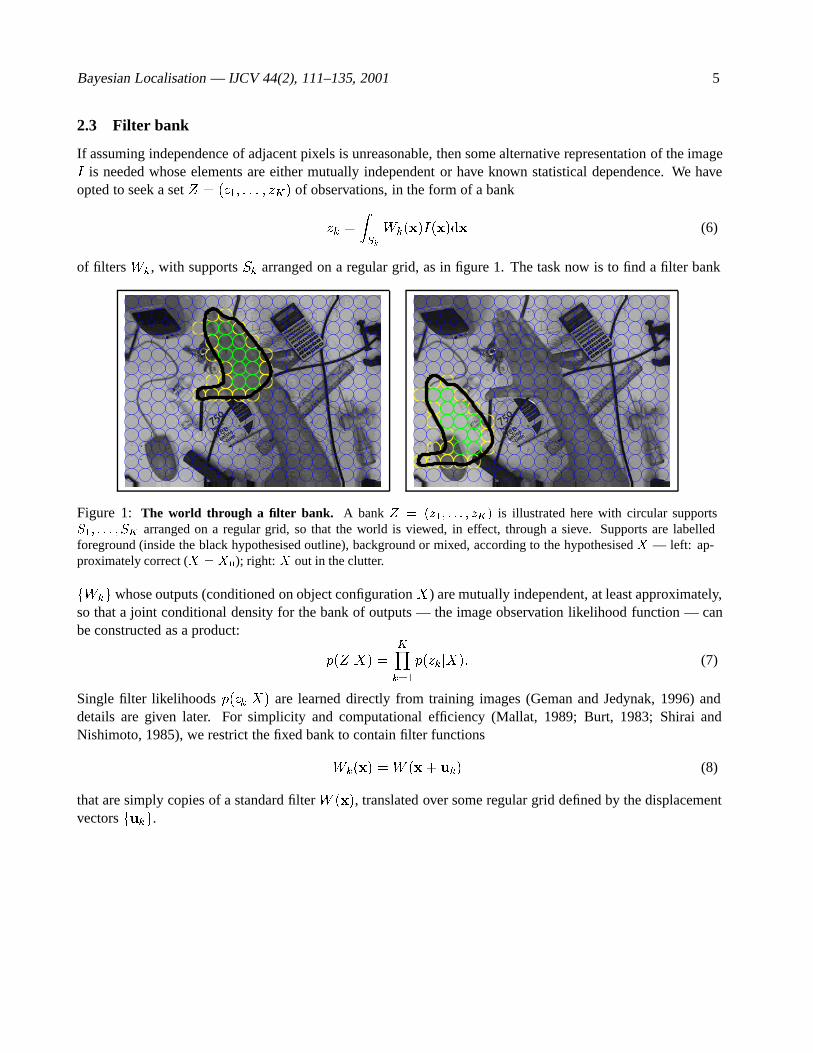
If assuming independence of adjacent pixels is unreasonable, then some alternative representation of the imageI is needed whose elements are either mutually independent or have known statistical dependence. We haveopted to seek a set Z = (z1; : : : ; zK) of observations, in the form of a bank

zk =

ZSk

Wk(x)I(x)dx (6)

of filters Wk, with supports Sk arranged on a regular grid, as in figure 1. The task now is to find a filter bank

Figure 1: The world through a filter bank. A bank Z = (z1; : : : ; zK) is illustrated here with circular supportsS1; : : : ; SK arranged on a regular grid, so that the world is viewed, in effect, through a sieve. Supports are labelledforeground (inside the black hypothesised outline), background or mixed, according to the hypothesised X — left: ap-proximately correct (X = X0); right: X out in the clutter.

fWkg whose outputs (conditioned on object configuration X) are mutually independent, at least approximately,so that a joint conditional density for the bank of outputs — the image observation likelihood function — canbe constructed as a product:

p(ZjX) =KYk=1

p(zkjX): (7)

Single filter likelihoods p(zkjX) are learned directly from training images (Geman and Jedynak, 1996) anddetails are given later. For simplicity and computational efficiency (Mallat, 1989; Burt, 1983; Shirai andNishimoto, 1985), we restrict the fixed bank to contain filter functions

Wk(x) =W (x+ uk) (8)

that are simply copies of a standard filter W (x), translated over some regular grid defined by the displacementvectors fukg.


2.4 Factored sampling

For the multi-modal distributions that arise with image observation likelihoods, Bayes’ formula (3) cannot becomputed directly but Monte-Carlo simulation is possible. In factored sampling (Grenander et al., 1991), ran-dom variates are generated from a distribution that approximates the posterior p(XjZ). A weighted “particle-set” f(s(1); �1); : : : ; (s(N); �N )g, of size N , is generated from the prior density p0(X) and each particle s(i)

is associated with a likelihood weight �i = f(si) where f(X) = p(ZjX). Then, an index i 2 f1; : : : ; Ngis sampled with replacement, with a probability proportional to �i; the associated si is effectively drawn froma distribution that converges (weakly) to the posterior, as N ! 1. It will prove useful later to express thesampling scheme graphically, as a “particle diagram”

p0N-

� f-

�

N- : (9)

It is interpreted as follows: the first arrow denotes drawing N particles from a known density p0, with equalweights �i = 1=N . (Particle sets are represented by open circles.) The � f operation denotes likelihoodweighting of a particle set:

�i ! f(s(i))�i; i = 1; : : : ; N:

The final step denotes sampling with replacement, as described above, repeated N times, to form a new set ofsize N in which each particle is given a unit weight; each particle is therefore drawn approximately from theposterior.

Where the likelihood f is a very narrow function in configuration space, sampling can become inefficient,requiring large N in order to give reasonable estimates of the posterior. In the paper (section 8) it is shownhow this can be mitigated by “layered sampling” in which broader likelihood functions are used in an advisorycapacity to “focus” the particle set down, in stages. In the vision context, layered sampling is a vehicle forimplementing multi-scale processing.

3 Probabilistic modelling of observations

The observation (ie output value) z from an individual filter is generated by integration over a support-set Ssuch as the circular one in figure 2, which is generally composed of both a background component B(X), anda foreground component F (X):

zjX =

ZB(X)

W (x)I(x) dx

| {z }MAIN NOISE SOURCE

+

ZF (X)

W (x)I(x) dx: (10)

The main source of variation in zjX is expected to come from the background which is assumed to be a samplefrom some general class of scenes. In contrast, the foreground relates to a given object, relatively preciselyknown, though still subject to some variability. This means that there should be a steady reduction in thevariance of the distribution of zjX as X changes from values in which the circular support is entirely overforeground, via intermediate locations overlapping both foreground and background, and finally to values inwhich it is entirely over background. This is supported by experiments in which density functions for z which


Object configuration

B(X)

F(X)

X

Figure 2: The support of a mask. A circular support set S is illustrated here, split into subsets F (X) from the foregroundand B(X) from the background.

have been learned from images, both from background regions and also from foreground regions (figure 3).The filter used in the experiment is a Gaussian

Figure 3: Learned observation densities for a Gaussian filter. Densities p(z) are exhibited both for foreground andbackground, in the case that W (x) is Gaussian, with support radius r = 20 pixels. Units of z are intensity, scaled so thatintensities in the original image lie in the range 0; 1.

G�(x) =1

�2exp�

jxj2

2�2(11)

in a circular support of radius r (= 3�).The role of p(zjX) in Bayesian localisation is as a likelihood function for X , associated with a particular

observation z, as illustrated in figure 4. Note that, although X is generally multidimensional, in the diagram itis depicted as a one-dimensional variable, for the sake of clarity. The entire family of idealised densities canbe represented in (z;X)-space as shown in the figure. Then, to construct the likelihood functions, the z-valueis considered to be fixed and X allowed to vary. This is illustrated in figure 4 by considering slices of constantz. For example, z = 2 in the figure depicts a relative high value which, in the example, is more likely to beassociated with a filter-support lying predominantly over the foreground. The resulting likelihood is peaked


0

0.2

0.4

−4−2

02

4

z

X0

0.2

0.4

−4−2

02

4

z

0

0.2

0.4 X

p(z|X)

foreground

Likeli

hood

Observation density

background foreground

background

z =2

z = −

1

Figure 4: Observation likelihood. The density p(zjX) is formally a function of z with X as a parameter, and isillustrated for foreground and background cases. The whole family of such one-dimensional densities, indexed by thecontinuous variableX , are assembled to synthesise p(zjX), as shown. Now p(zjX) is “sliced” in the orthogonal direction,to generate likelihoods (functions of X for fixed z). In the examples, an observation z = 2 biases X towards a foregroundvalue, whereas z = �1 biases towards background.

around a value of X corresponding to predominant foreground support. Conversely, for z = �1, the support ismore likely to be predominantly over the background and the mode of the likelihood shifts towards backgroundvalues of X . 3

Likelihood functions from several observations zk should “fuse” when they are combined (7), to forma joint likelihood that is more acutely tuned (figure 5) than the likelihood for any individual zk. Note theimportance of the zk from “mixed” supports, lying partly on the background and partly on the foreground. Itmight be tempting to regard them as contaminated and discard them whereas, in fact, they should be especiallyinformative, responding selectively to the boundary of the object — see figure 1.

4 Filter response-learning

If it were not for mixed supports, learning would be relatively straightforward. Over the background, forinstance, it would be sufficient just to evaluate the outputs z (6) of the circular filter repeatedly, at assorted

3Note that “slicing” is purely an analytical tool to illustrate the way observation likelihoods exist implicitly within a probabilisticmodel for filter response. Slicing does not actually form part of any algorithm proposed here.


p(z |X)

p(z |X)

p(z |X)

p(z ... z |X)

z

z

z

1

3 2

1

2

3

1

X

X

X

XX0

3

Figure 5: “Hyperacuity” from pooled observations. Likelihoods from independent observations combine multiplica-tively, to give a joint likelihood narrower than any of the individual constituents.

locations over some training image, and fit a probability distribution pB(z). However, over a mixed support,only a part of the circle lies over the background. If this part is approximated as a segment of a circle (figure6), and provided each filter functional Wk(x) is isotropic (or steerable (Perona, 1992)), then the background

approxB(X)

F(X)

B(X)

F(X)

ρ2r

2r

object

object outline

Figure 6: Approximating foreground/background supports Assuming that the object’s bounding contour is suffi-ciently smooth (on the scale r of the radius of the filter support) the boundary between foreground and background can beapproximated as a straight line. The support therefore divides into segments with offsets 2r� and 2r(1��) for backgroundand foreground respectively.

distribution can be parameterised by a single offset parameter � (at a given scale r). This parameter is defined


for 0 � � � 1, as in the figure so that: when � = 1 the filter support is entirely over the background; when� = 0 it is entirely over the foreground; and for 0 < � < 1 it straddles the object boundary.

Training examples for background learning must be constructed over circular segments with offsets through-out the range 0 � � � 1, to learn background distributions pBk (zj�). (Clearly, in practice, only a finite numberof these can be learned, leaving the continuum of � to be filled in by interpolation.) To consider a hypoth-esised configuration X , the Bayesian localisation algorithm needs to evaluate, for each k, an offset function�k(X) and a likelihood pk(zj�k(X)). The likelihood function consists of a sum of background and foregroundcomponents, and is therefore constructed as a (numerically approximated) convolution

pk(zj�) = pBk (zj�) � pFk (zj�) (12)

of learned background and foreground density functions.

5 Learning the background likelihood

Statistical independence of image features is an issue that has been studied elsewhere, in the context of neuralcoding (Field, 1987): if neural codes are efficient in the sense of avoiding redundancy, their components can beexpected to be nearly statistically independent. It is also known that independent components of natural scenestend to have “sparse” or “hyper-kurtotic” distributions — ones with extended tails compared with those of anormal distribution (Bell and Sejnowski, 1997).

5.1 Experiments with response correlation

Experiments on background correlation are done here using statistics collected from each of the four scenesin figure 7. Our experiments are similar to those done by Zhu and Mumford (1997) in which they showed thebackground distribution is remarkably consistent across scenes, for a rG filter. Here we look at the div of thatfilter output, which should therefore similarly show a consistent distribution, and the small-scale experimentsdone here support that. A necessary condition for independence is freedom from correlation, so autocorrelationwas estimated by random sampling of pairs of supports, separated by a varying displacement. This was done fortwo choices of filter function W (x): Gaussian G(x) and Laplacian of Gaussian r2G(x), and typical resultsare shown in figure 8. At a displacement such as r (= 3�), corresponding to a typical separation betweenfilters, the G(x) filter shows correlation and hence there cannot be independence. On the other hand r2G(x)is uncorrelated at a displacement of r. Further experiments, looking at the entire joint distribution for responseszk; zl of two filters with variable spatial separation, support statistical independence, as figure 9 shows.

The independence is obtained at the cost of throwing away information about mean response and the 1stmoment, though this is likely to be beneficial in conferring some invariance to illumination variations. Theseexperiments were for complete, circular supports. With part-segments of a circle (� < 1), statistical inde-pendence of r2G(x) responses deteriorates. Experiments like the ones in figure 8 show correlation lengthsincreasing for � < 1, with � = 1

4 the worst case. This will mean greater statistical dependence between mixedsupports, and it is not clear how this could be improved; but note at least that typically it is a minority of filtersupports that are mixed.


Figure 7: Background learning: training scenes used in experiments.

Fitting the background distribution

A further benefit of the r2G(x) filter is that the learned background distributions turn out to be far moreconstant across scenes(and this is known to be true also for rG filters (Zhu and Mumford, 1997)) than for aplainG(x) filter. Background distributions were learned by repeated sampling of zk (6) for randomly positionedsupports, then histogramming and smoothing to estimate pB(z). The results for complete circular supports(� = 1), shown in figure 10, show sufficient consistency to indicate that some fixed parametric form shouldbe sufficient to represent the densities. The learned responses turn out not to be normally distributed, but havea hyper-kurtotic distribution, that is one with greater kurtosis than a normal distribution, and this is clearlyvisible in the extended tails in figure 10. Hyper-kurtotic distributions are known to emerge in independentcomponents of images (Bell and Sejnowski, 1997), and are often found to be well modelled by a single-exponential distribution4

pB(z) / exp�jzj=�: (13)

The distribution fits the experimental data quite well (figure 11). In that case, a global background likelihood

4We refrain from the commonly used term “Laplace” distribution here, to avoid the potential confusion with the Laplacian operatorinr2G.


1

correlation

displacement (pixels)

Gaussian

Laplacian

050 100

r = 10 correlation


Gaussian

Laplacian

0

1 r = 20

50 100

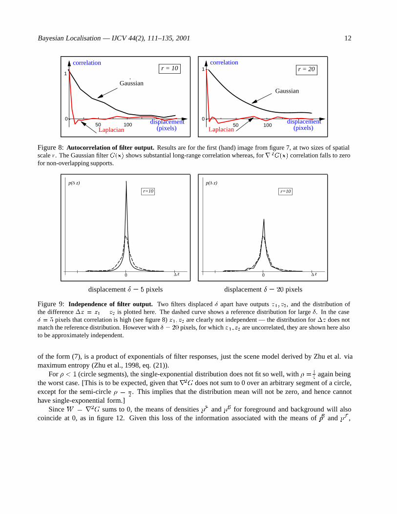
Figure 8: Autocorrelation of filter output. Results are for the first (hand) image from figure 7, at two sizes of spatialscale r. The Gaussian filter G(x) shows substantial long-range correlation whereas, for r 2G(x) correlation falls to zerofor non-overlapping supports.

∆

0 z∆

p( z)

r=10

∆

0 z∆

p( z)

r=10

displacement � = 5 pixels displacement � = 20 pixels

Figure 9: Independence of filter output. Two filters displaced � apart have outputs z1; z2, and the distribution ofthe difference �z = z1 � z2 is plotted here. The dashed curve shows a reference distribution for large �. In the case� = 5 pixels that correlation is high (see figure 8) z1; z2 are clearly not independent — the distribution for �z does notmatch the reference distribution. However with � = 20 pixels, for which z 1; z2 are uncorrelated, they are shown here alsoto be approximately independent.

of the form (7), is a product of exponentials of filter responses, just the scene model derived by Zhu et al. viamaximum entropy (Zhu et al., 1998, eq. (21)).

For � < 1 (circle segments), the single-exponential distribution does not fit so well, with � = 14 again being

the worst case. [This is to be expected, given that r2G does not sum to 0 over an arbitrary segment of a circle,except for the semi-circle � = 1

2 . This implies that the distribution mean will not be zero, and hence cannothave single-exponential form.]

Since W = r2G sums to 0, the means of densities pF and pB for foreground and background will alsocoincide at 0, as in figure 12. Given this loss of the information associated with the means of pB and pF ,


z B

Bp(z )

0 z B

Bp(z )

0

Gaussian G(x) Laplacian of Gaussian r2G(x)

Figure 10: Learned background distributions. Learned densities pB(z) are shown here for each of the four scenes infigure 7 at scale r = 20: they are highly variable for the G(x) filter, but rather consistent for r 2G(x).

z

p (z)B

z

p (z)B

Figure 11: Exponential model for background distributions. Learned densities pB(z) for the first and last of the 4scenes in figure 7, at scale r = 20 with � = 1, are fitted here (by MLE) to an exponential distribution, which captures theelongation of the tails.

discriminability between foreground and background is reduced, the price paid for improved illumination-invariance. However, the foreground model can be extended in certain ways to improve discriminability again.One way is “foreground subdivision” as in section 6; another uses intensity templates (Sullivan and Blake,2000).

z

p(z|X)

foreground

background

Figure 12: Foreground and background distributions whenRW (x)dx = 0, for support radius r = 20 pixels. The

means of the foreground and background distributions now coincide, cf. figure 3.


5.2 Optimal filter bank grid

At a given spatial scale, the maximum information about an image can be collected by packing filter supportsSk as densely as possible, within the constraint that filter outputs zk must be uncorrelated. For filtersWk that areisotropic, correlation depends simply on the displacement between pairs of filters. A useful measure is that thecorrelation function (figure 8) crosses 0 at a displacement of around r (= 3�). The most effective packing offilters, for the given level of correlation, will be the one that maximises the packing density for a given minimumdisplacement between filter centres. This is well-known to be a hexagonal tesselation, whose packing densityis approximately 50% greater than square packing. For the r2G filter, the filter support is circular5 with radiusapproximately r (= 3�) which is also the displacement for (approximately) zero correlation. Hence supportsin the hexagonally tesselated optimal filter bank overlap substantially as in figure 13.

Figure 13: Optimal tesselation of filter supports. Maximum density ofr2G filters, while avoiding correlation betweenfilter pairs, is achieved by a hexagonal tesselation, as shown, with substantial overlap (support radius r = 40 pixelsillustrated).

6 Learning the foreground likelihood

Learning distributions for foreground responses is similar to the background case. As before, pF (zj�) is learnedfor some finite set of �-values, and interpolated for � 2 [0; 1]. There are some important differences however.

5Of course, the filter has theoretically unbounded support, but we take the point at which filter amplitude falls to around 10% of itsmaximum value.


6.1 Deformations and pooling

Three-dimensional transformations and deformations of the foreground object must be taken into account. Tab-ulating pF not only against � but also against transformation parameters is computationally infeasible. Varia-tions that cannot be modelled parametrically can nonetheless be pooled into the general variability representedby pF (zj�). This implies that pF (zj�) should be learned not simply from one image, but from a training set ofimages containing a succession of typical transformations of the object.

6.2 Outline constraint

The distribution pB(zj�) was learned from segments dropped down at random, anywhere on the background.Over the foreground, in the case that � = 0, pF (zj�) is similarly learned from a circular support, dropped nowat any location wholly inside the training object. However, whenever � > 0, the support F (X) must touch theobject outline; therefore, for 0 < � < 1, pF (zj�) has to be learned entirely from segments touching the outline.

6.3 Foreground subdivision

For � = 0, it has so far been proposed that pF (zj�) be learned by pooling responses throughout the objectinterior. Pooling in this way discards information contained in the gross spatial arrangement of the grey-levelpattern. Sometimes this provides adequate selectivity for the observation likelihood, particularly when theobject outline is distinctive, such as the outline of a hand as in figure 1. The outline of a face, though, is lessdistinctive. In the extreme case of a circular face, and using isotropic filters, rotating the face would not produceany change in the pooled response statistics. In that case, the observation likelihood would carry no informationabout (2D) orientation. One approach to this problem is to include some anisotropic filters in the filter bank,which would certainly address the rotational indeterminacy.

An alternative approach which also enhances selectivity generally, is to subdivide the interior F of theobject as F = F0 [ : : : [ FNF

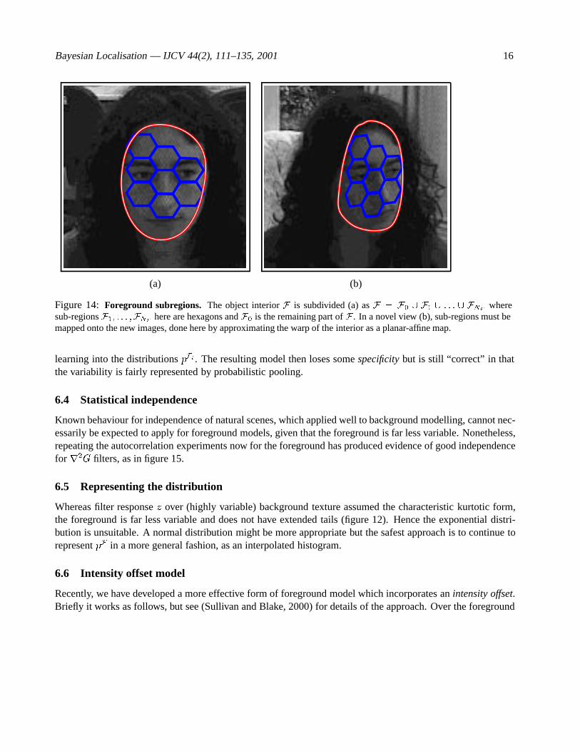
, as in figure 14, and construct individual distributions pFi(zj� = 0) for eachsubregion Fi . A foreground distribution pFi(zj� = 0) applies to any filter support Sk that lies entirely withinF and whose centre is in Fi. The case i = 0 is a “catch-all” region, pooling the responses of any filter whosecentre is not in Fi for any i > 0 (the hexagons in figure 14). The choice of the number NF of sub-regions is ofcourse a trade-off between increasing, with NF , the specificity of the information that is learned while, at thesame time, requiring more data to learn adequate estimates of the pFi as the sub-regions Fi get smaller.

Sub-regions are defined with respect to a standard configuration, say X = 0, as in figure 14a. In a novelconfiguration X 6= 0, encountered either in training or evaluation of the likelihood p(ZjX), suitably warpedforms of Fi must be defined (figure 14b)). This could be achieved by defining the configuration space Xas a space of two-dimensional warps gX , using thin plate splines for example (Bookstein, 1989). A moreeconomical but more approximate approach is adopted here, representing the outline contour as a parametricspline curve (Bartels et al., 1987), and the configuration-space X is modelled as a sub-space of the splinespace. Then the warp of the interior of the object is approximated as an affine transform by projecting theconfiguration X onto a space of planar-affine transformations (Blake and Isard, 1998, ch 6). The fact that thisaffine transformation warps the interior only approximately does not imply that errors are introduced into theBayesian localisation procedure. Rather, the variability due to approximating the warp is simply pooled during


(a) (b)

Figure 14: Foreground subregions. The object interior F is subdivided (a) as F = F0 [ F1 [ : : : [ FNF wheresub-regions F1; : : : ;FNF here are hexagons and F0 is the remaining part of F . In a novel view (b), sub-regions must bemapped onto the new images, done here by approximating the warp of the interior as a planar-affine map.

learning into the distributions pFi . The resulting model then loses some specificity but is still “correct” in thatthe variability is fairly represented by probabilistic pooling.

6.4 Statistical independence

Known behaviour for independence of natural scenes, which applied well to background modelling, cannot nec-essarily be expected to apply for foreground models, given that the foreground is far less variable. Nonetheless,repeating the autocorrelation experiments now for the foreground has produced evidence of good independencefor r2G filters, as in figure 15.

6.5 Representing the distribution

Whereas filter response z over (highly variable) background texture assumed the characteristic kurtotic form,the foreground is far less variable and does not have extended tails (figure 12). Hence the exponential distri-bution is unsuitable. A normal distribution might be more appropriate but the safest approach is to continue torepresent pF in a more general fashion, as an interpolated histogram.

6.6 Intensity offset model

Recently, we have developed a more effective form of foreground model which incorporates an intensity offset.Briefly it works as follows, but see (Sullivan and Blake, 2000) for details of the approach. Over the foreground


0

correlation


r = 20

20 40

1.0

0

correlation


r = 20 1.0

20 40

Figure 15: Foreground autocorrelation for the r2G filter, over two different foreground objects: a hand (left) anda face (right). In both cases, correlation falls to zero at a displacement of around r or 3�, similarly to correlation ofbackground texture.

F(X), the intensity I(x) is modelled as having a mean �IX(x) generated as a warp

�IX(x) = �I(TX(x))

of a learned intensity template �I(x). This then leaves only the difference

�IX(x) = I(x)� �I(TX(x)); x 2 F(X);

as observed by the filter bank fWkg, to be modelled statistically. More of the variation in the intensity patternI(x); x 2 F(X) is accounted for deterministically, leaving a tighter distribution for the random componentof the foreground model.

Inclusion of the intensity offset, in this way, fulfils a similar objective to the foreground subdivision ofsection 6, in using more of the information in the spatial intensity pattern of the object. It turns out (Sullivanand Blake, 2000) to have an additional advantage: that the template model can be extended to take some accountof lighting variations deterministically, rather than leaving lighting changes to be modelled entirely statistically.

7 Exercising the learned observation likelihood

Having established, in previous sections, that reasonable densities pk(zjr) for individual supports can be learnedfrom background and foreground densities, it is now possible to exercise the full joint likelihood functionp(ZjX). This is constructed (7) as a product, in which the offset � for each support segment is obtained fromits offset function �k(X):

p(ZjX) =KYk=1

pk(zkj�k(X)): (14)

Evaluation of the offset function requires a geometrical calculation of the size of the circle-segment that ap-proximates the intersection of the object (at configuration X) with the kth support. It is interesting to notethat, although Bayesian analysis requires that Z should consist of the entire set of filters zk in figure 1, someeconomies can legitimately be made. Given a sample X1; : : : ;XN of object hypotheses, if some filter supportSk lies always in the background for all the Xn, the corresponding term can be factored out of (14). For a


truly parallel, pyramid architecture this may be no real advantage. If image processing is serial a “samplingrehearsal” can tag just those zk whose likelihoods do not factor out; other zk need not be computed. The“factoring out” phenomenon also makes another interesting point. The filters that actually contribute to globallikelihood variations are those near the boundary of at least some hypothesised configuration X; so despitebeing intensity-based, it transpires that Bayesian localisation does in fact emphasise edge information.

The learned observation likelihood is exercised here in two ways. First, the likelihood function is exploredsystematically, with respect to translation, rotation etc., and at various spatial scales. Secondly, the likelihoodfunction is applied to randomly generate samples, to sweep out posterior distributions for pose, again at severalscales.

7.1 Systematic variations in observation likelihood

First, for the hand scene of figure 1, p(ZjX) — the joint likelihood composed of a product of likelihoodsp(zkjX) for individual filters, is exercised systematically. This is done as a check that the likelihood doesregister a peak at the true object position, and has reasonable variations around the peak. In these demon-strations, X is varied over a configuration space of Euclidean similarities; results are displayed in figure 16.The joint likelihood fuses information from individual supports effectively, with a maximal value, as expected,

0 50 Translation (pixels)

−50

Likelihood r=20 pixels

0 Rotation(degrees)

−90 90


0.5 1 1.5

Scaling factor


Translation Rotation Scaling

Figure 16: Exercising the joint likelihood. The joint observation likelihood p(ZjX) is exercised here as X rangesover coordinate axes in the space of Euclidean similarities. Note that the peak in each case is approximately at the origin(X = X0). (Support radius is r = 20 pixels.)

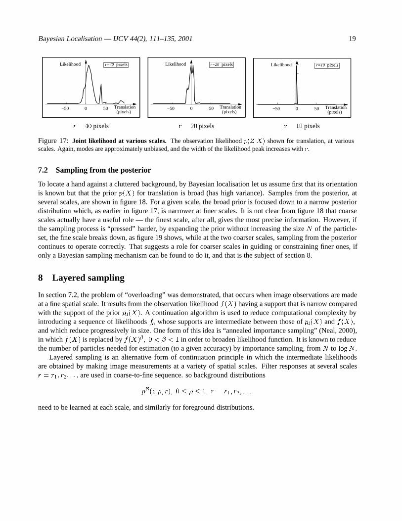
near the true solution X0. Figure 17 demonstrates the effect of changing the filter scale r. As expected, thelikelihood function is more broadly tuned at coarser scales, appearing to have a width of about 2r, or less dueto hyperacuity effects as in figure 5. As a final check, it is interesting to consider the likelihood ratio for twoconfigurations, one correctly positioned over the target, and one way out over background as in figure 1. Insuch cases, treating pixels as independent typically produces ridiculously large likelihood ratios. Even usingGaussian masks (r = 20), which we know are not independent, gives a likelihood ratio in this case of 1 : 1055

— still very large. However, this falls considerably with r2G masks, as expected given the independence oftheir output over foreground and background, to a more plausible 1 : 104

To summarise, the learned observation likelihood for r2G masks has been exercised here, systematically,and found to have reasonable properties. The next task is to use it to compute approximations to the posteriorp(XjZ), by means of the factored sampling scheme of section 2.4.



−50

Likelihood pixelsr=40


−50



−50

Likelihood pixelsr=10

r = 40 pixels r = 20 pixels r = 10 pixels

Figure 17: Joint likelihood at various scales. The observation likelihood p(ZjX) shown for translation, at variousscales. Again, modes are approximately unbiased, and the width of the likelihood peak increases with r.

7.2 Sampling from the posterior

To locate a hand against a cluttered background, by Bayesian localisation let us assume first that its orientationis known but that the prior p(X) for translation is broad (has high variance). Samples from the posterior, atseveral scales, are shown in figure 18. For a given scale, the broad prior is focused down to a narrow posteriordistribution which, as earlier in figure 17, is narrower at finer scales. It is not clear from figure 18 that coarsescales actually have a useful role — the finest scale, after all, gives the most precise information. However, ifthe sampling process is “pressed” harder, by expanding the prior without increasing the size N of the particle-set, the fine scale breaks down, as figure 19 shows, while at the two coarser scales, sampling from the posteriorcontinues to operate correctly. That suggests a role for coarser scales in guiding or constraining finer ones, ifonly a Bayesian sampling mechanism can be found to do it, and that is the subject of section 8.

8 Layered sampling

In section 7.2, the problem of “overloading” was demonstrated, that occurs when image observations are madeat a fine spatial scale. It results from the observation likelihood f(X) having a support that is narrow comparedwith the support of the prior p0(X). A continuation algorithm is used to reduce computational complexity byintroducing a sequence of likelihoods fn whose supports are intermediate between those of p0(X) and f(X),and which reduce progressively in size. One form of this idea is “annealed importance sampling” (Neal, 2000),in which f(X) is replaced by f(X)� ; 0 < � < 1 in order to broaden likelihood function. It is known to reducethe number of particles needed for estimation (to a given accuracy) by importance sampling, from N to logN .

Layered sampling is an alternative form of continuation principle in which the intermediate likelihoodsare obtained by making image measurements at a variety of spatial scales. Filter responses at several scalesr = r1; r2; : : : are used in coarse-to-fine sequence. so background distributions

pB(zj�; r); 0 � � � 1; r = r1; r2; : : :

need to be learned at each scale, and similarly for foreground distributions.


prior posterior: r = 40 pixels

posterior: r = 20 pixels posterior: r = 10 pixels

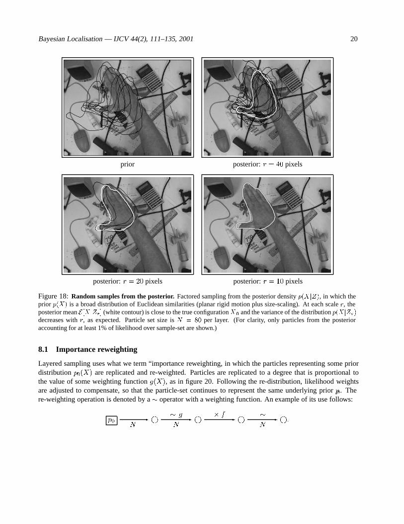
Figure 18: Random samples from the posterior. Factored sampling from the posterior density p(X jZ), in which theprior p(X) is a broad distribution of Euclidean similarities (planar rigid motion plus size-scaling). At each scale r, theposterior mean E [X jZr] (white contour) is close to the true configurationX0 and the variance of the distribution p(X jZr)decreases with r, as expected. Particle set size is N = 80 per layer. (For clarity, only particles from the posterioraccounting for at least 1% of likelihood over sample-set are shown.)

8.1 Importance reweighting

Layered sampling uses what we term “importance reweighting, in which the particles representing some priordistribution p0(X) are replicated and re-weighted. Particles are replicated to a degree that is proportional tothe value of some weighting function g(X), as in figure 20. Following the re-distribution, likelihood weightsare adjusted to compensate, so that the particle-set continues to represent the same underlying prior p0. There-weighting operation is denoted by a � operator with a weighting function. An example of its use follows:

p0N-

� g

N-

� f-

�

N- :


prior posterior: r = 40 pixels

posterior: r = 20 pixels posterior: r = 10 pixels

Figure 19: A broader prior “overloads” factored sampling Now the demonstration of figure 18 is repeated, butwith a prior 1.5 times as broad, causing sampling at the finest scale to break down (observe the large bias in the meanconfigurations at scale r = 10; 20 pixels. (Again, N = 80.)

This is factored sampling (9) with an extra, intermediate, reweighting stage. In terms of particle-sets, thereweighting operation � g is defined as follows

f(s(i); �i); i = 1; : : : ; Ng ! f(s(i(j)); 1=g(s(i(j)))); j = 1; : : : ; Ng

where each i(j) is sampled with replacement from i = 1; : : : ; N with probability proportional to �ig(s(i)).A useful property of the resampling operation � g is that it is an asymptotic identity: as N ! 1, the

difference between the distributions of the two random variables generated by

p0N-

�

1- and by p0

N-

� g

N-

�

1-

converges weakly to 0.


X

g(X)

0p (X)

~ g

0p (X)

Figure 20: Importance reweighting. A uniform prior p0(X), represented as a particle-set (top), is resampled via animportance function g to give a new, re-weighted particle-set representation of p 0. (The illustration here is for a one-dimensional distribution, though practically X is multidimensional.)

Resampling with the � g operation does not, on its own, deal with the problem of a narrow likelihoodfunction. Although it does concentrate sampling to a narrower region of configuration space, the gaps betweenparticles are as great as ever (figure 21). Gaps can be filled, however, by adding a further random variable

g(X) ~ g

f(X)

X* p

p

* p

p 0

1

0

10p

Figure 21: Resampling followed by convolution. This simplified example illustrates that importance reweighting onits own cannot repopulate the sparsely sampled support of the likelihood f . Repopulation can however be achieved byadding a random increment, corresponding to convolving the prior p 0 with p1, the density of the random step.

with density p1, to each particle. This has the effect of diffusing apart identical copies of particles generated inthe resampling step. Of course, the combined operation is no longer an asymptotic identity — particles at theoutput of

p0N-

� g

N-

� p1-

�

1-

are distributed asymptotically according to the density p0 � p1.


8.2 The layered sampling algorithm

Layered sampling is applicable when importance resampling functions f1; : : : ; fM are available, in whichfM = f is the true likelihood, and each fm�1 is a coarse approximation to fm. In addition, the prior p0must be decomposable as a series of convolutions

p0 = p00 � p01 : : : � p

0M�1 (15)

and this corresponds to expressing X a priori as a sum of random variables. Functional forms for the densitiesp0m need not necessarily be known, provided only that a random sample generator can be constructed for each.For example, in processing motion sequences using the CONDENSATION algorithm (Isard and Blake, 1996),p00 could be represented as a set of particles from the previous time t � 1, and pd = p01 : : : � p

0M�1 is some

decomposition of a normal distribution pd(X(t)jX(t� 1)) for the likely displacement over one time-step, intonormally distributed components. With this decomposition of the prior, the sampling process (9) on page 6 canbe replaced by a sequence of layers:

p00 N-

� f1

N-

� p01-

: : :

� fM�1

N-

� p0M�1-

� fM-

�

N- :

(16)

Each layer includes an importance resampling step, with the observation likelihood fi at the ith scale as theresampling function, until theM th and final layer, at which the fine-scale fM acts multiplicatively on likelihoodweights, in the usual way.

The asymptotic correctness of layered sampling can be demonstrated by manipulating the sampling dia-gram. Using the asymptotic identity property of �, (16) can be rewritten, deleting resampling links, to give

p00 N-

� p01-

: : :

� p0M�1-

� fM-

�

N- :


and now the p0m convolutions can be composed to give

p00 � p01 � : : : � p

0M�1 N

- � fM-

�

N- :

which, from (15), and since fM = f , reduces to the original factored sampling process (9).

8.3 Variance reduction

A remaining problem is how to choose the likelihood functions and the decomposition of pd in such a way asto minimise the variance of the particle set generated in the final layer. These are complex problems in general,but some progress can be made by setting out the following special case.

1. The prior p00 is a rectangular distribution, with a support of volume a0 in configuration space.

2. Each likelihood function fm is idealised as a rectangular (uniform) distribution with a support of volumeam.

3. The support of each fm is a subset of the support of fm�1.

4. Each p0m is chosen in such a way that N particles are effectively uniformly distributed over the supportof fm, as depicted in figure 21. This can be done by matching the support of p0m�1 to the support of fm.

5. Variance minimisation is not well-posed for rectangular distributions fm, since their support is bounded.Instead, we minimise the “failure rate” — the probability that the particle set in some layer is empty.

Under these assumptions it can be shown (see appendix) that the failure rate is minimised by choosing

am�1 = �am (17)

so that successive support volumes are in some fixed ratio �.Three further useful results (derivations omitted) can be obtained using analysis of estimator variance for

importance sampling (Neal, 2000; Liu and Chen, 1995; Geweke, 1989).

� Using just a single layer (i.e. without layered sampling), the number N of particles required to achieve agiven failure rate is

N / a0=aM (18)

� With layered sampling, the failure rate is minimised by having approximately

M = log2(a0=aM ) (19)

layers. This means that � = 1=2 is the optimal ratio of support volumes.

� With the optimal number M of layers, the total number of particles required falls to

NM / log2(a0=aM ); (20)

a logarithmic speed-up compared with (18).


9 Results

Layered sampling is applied here to the problem of multi-scale localisation. In all cases, a hexagonal tesselationof filters was used with separations of 6� (sections 9.1, 9.2) or 3� (sections 9.3, 9.4). [Recall that the supportof the filters are truncated at r = 3�; filter sizes are specified as r-values in experiments below.] A constantnumber N of particles was used in each layer; demonstrations with motion in section 9.4 were done with just asingle layer, though clearly these also would be expected to benefit from multiple layers.

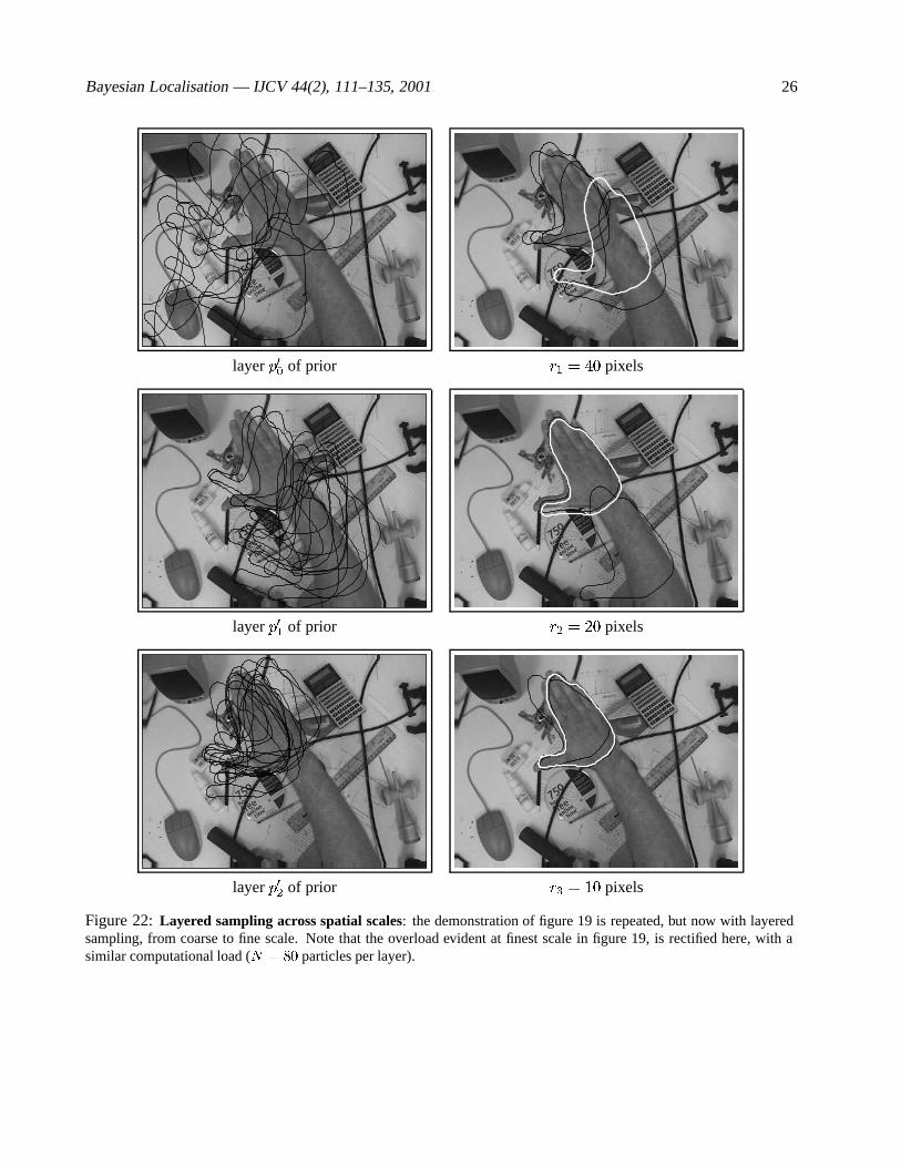
9.1 Sampling across scales

In the Bayesian localisation application, the fm from the layered sampling algorithm correspond to observationlikelihoods from the coarsest scale m = 1 to the finest m = M . Operation of the algorithm is illustratedhere, in figure 22, for the hand-finding problem that caused the overloading of single-scale sampling earlier, insection 7.2. The normally distributed prior p0 is split, as a sum of normal variables, into 3 factors

p0 = p00 � p01 � p

02;

each factor to be used before scales r1; r2; r3 in the coarse-to-fine hierarchy of observations. Scales arechosen to decrease geometrically, as implied by the fixed ratio rule (17) above. (This implication holds on theassumption that observation likelihood functions scale linearly with filter radius r, and demonstrations tend tosupport this, as in figure 17). The ith scale generates an observation likelihood function fi, where fi(X) =p(ZijX). Note that the formal likelihood derives from observations only at the finest scale. Observations atother scales are cast by layered sampling in an “advisory” role, their scope limited to importance sampling forthe next finer scale. This avoids any need for any formal assumption of statistical independence across scaleswhich may be hard to justify.

9.2 Occlusion

One of the attractions of intensity-based matching is its robustness to disturbances in the image data, and asevere form of disturbance is presented by occlusion. Where occlusion is anticipated, this is addressed in theBayesian localisation framework simply by treating the occluder as part of the background, and evaluating theappropriate observation-likelihood functions there. More challenging is occlusion that is not anticipated, asin figure 23. The figure illustrates the power of the Bayesian sampling approach to deal with ambiguity. Atcoarse scale, the part-occluded and blurred representation of shape leaves object-orientation quite ambiguous,though translation is somewhat constrained. Finer scales contain fragments of curve at sufficient resolution toregister quite precisely with part of the object outline. Hence the rotational ambiguity is resolved. Even thoughthe posterior at the finest scale has very small variance, nonetheless, the facility to represent ambiguity in theintermediate processes is what has allowed multi-scale information to be propagated effectively.

9.3 Pose variation

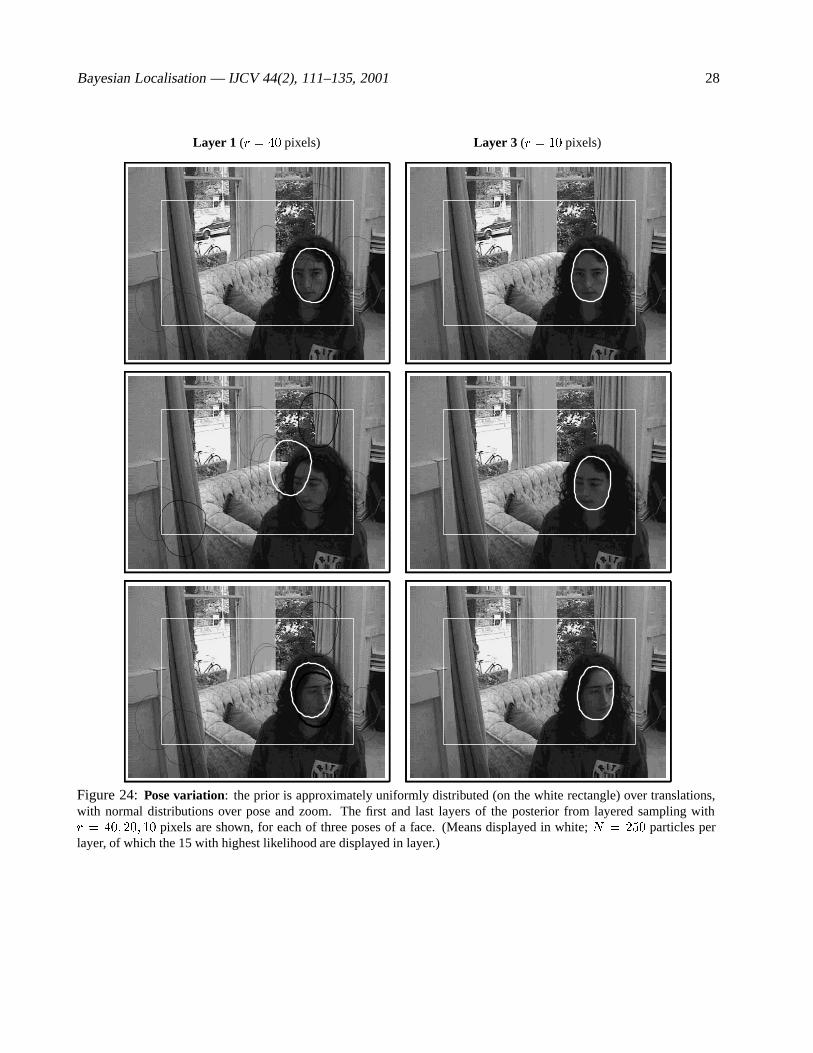
Bayesian localisation is capable of handling a configuration space X that incorporates varying 3D pose, asthe demonstration of figure 24 shows. The foreground distributions in this demonstration were learned using


layer p00 of prior r1 = 40 pixels



Figure 22: Layered sampling across spatial scales: the demonstration of figure 19 is repeated, but now with layeredsampling, from coarse to fine scale. Note that the overload evident at finest scale in figure 19, is rectified here, with asimilar computational load (N = 80 particles per layer).





Figure 23: Layered sampling with occlusion: a demonstration like the one in figure 22 but now with the object sufferingunpredicted occlusion. Note that, at the coarsest scale, shape information is sufficiently distorted by occlusion, that objectorientation is quite ambiguous in the posterior. Finer scales resolve the ambiguity.


Layer 1 (r = 40 pixels) Layer 3 (r = 10 pixels)

Figure 24: Pose variation: the prior is approximately uniformly distributed (on the white rectangle) over translations,with normal distributions over pose and zoom. The first and last layers of the posterior from layered sampling withr = 40; 20; 10 pixels are shown, for each of three poses of a face. (Means displayed in white; N = 250 particles perlayer, of which the 15 with highest likelihood are displayed in layer.)


foreground subdivision as discussed in section 6, with subregions of a diameter equal to that of the filter support.In fact, in the coarsest layer, there is space within the face contour for only one subregion, but 7 subregions atr = 20 and 33 at r = 10. Note the “rogue” face hypothesis appearing on the curtain at the left, which receivesa significant weight in layer 1, at the coarsest scale (a blurry hallucination), but does not survive at fine scale.

A further demonstration of face-tracking, free-running at about 1 frame/sec, is given at

http://www.robots.ox.ac.uk/˜vdg/movies/bayes-face.mpg.

In this case there are two layers with r = 40; 20 and N = 600 particles per layer, and a foreground intensitymodel is used, as in (Sullivan and Blake, 2000).

9.4 Motion tracking

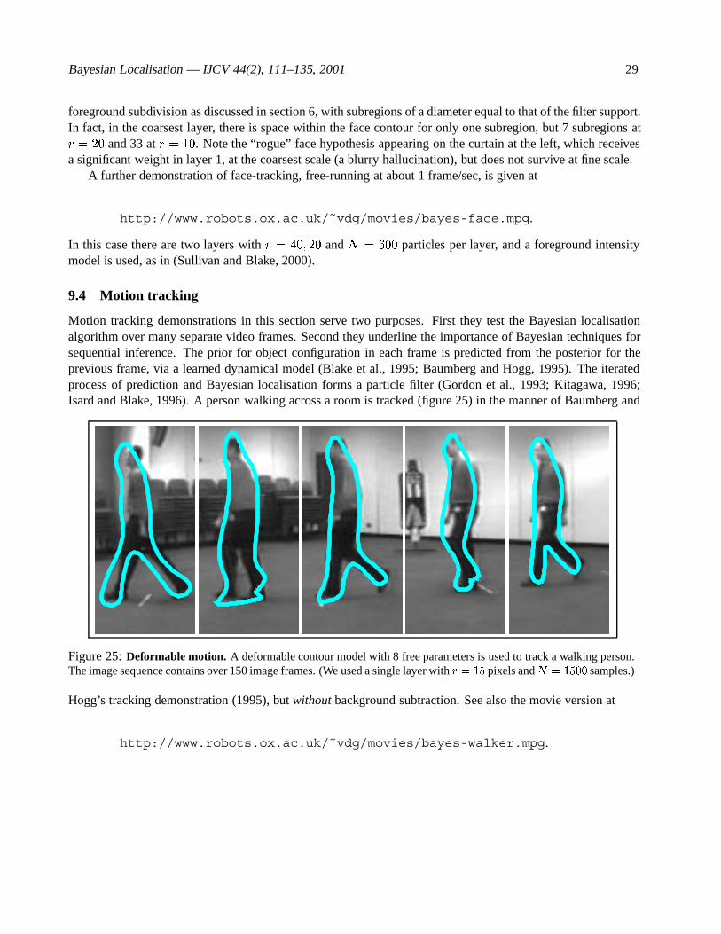
Motion tracking demonstrations in this section serve two purposes. First they test the Bayesian localisationalgorithm over many separate video frames. Second they underline the importance of Bayesian techniques forsequential inference. The prior for object configuration in each frame is predicted from the posterior for theprevious frame, via a learned dynamical model (Blake et al., 1995; Baumberg and Hogg, 1995). The iteratedprocess of prediction and Bayesian localisation forms a particle filter (Gordon et al., 1993; Kitagawa, 1996;Isard and Blake, 1996). A person walking across a room is tracked (figure 25) in the manner of Baumberg and

Figure 25: Deformable motion. A deformable contour model with 8 free parameters is used to track a walking person.The image sequence contains over 150 image frames. (We used a single layer with r = 15 pixels andN = 1500 samples.)

Hogg’s tracking demonstration (1995), but without background subtraction. See also the movie version at

http://www.robots.ox.ac.uk/˜vdg/movies/bayes-walker.mpg.


Instead, distracting background clutter is dealt with by the learned foreground/background models embodied inthe observation likelihood. Consequently, the method not limited to backgrounds that are stationary, or movingin some easily predictable fashion.

A note should be added here on computation time. The task (on-line, excluding learning) here consistsprincipally of image processing to obtain the zk, and of computation of likelihood (14), of which the offsetfunction pn(zkj�k(X)) is main burden. The image processing can be done using pyramid filter banks (Burt,1983) that are available in hardware. The offset function (at scale r = 40) can be computed for approximatelyN = 500 particles per time-step, at frame-rate. Bayesian localisation at video frame-rate is therefore quitefeasible, in principle.

10 Conclusions

The original elements of Bayesian localisation are: the development of filter-based likelihood functions formatching with particular attention to statistical independence; learning of foreground and background distri-butions, and distributions for “mixed” receptive fields; probabilistic multi-scale analysis by means of “layeredsampling”.

The approach has been tested on a variety of foregrounds and backgrounds. It is capable of planar ob-ject localisation, even with unpredicted occlusion, and versatile enough to work with 3D pose changes, andwith image sequences of moving objects, including nonrigid ones. A number of issues are raised: the choiceof partition for the prior in layered sampling; the use of spatio-temporal filters and associated independencearguments; temporal updating of the foreground distribution. These remain for future investigation.

Acknowledgements

We are grateful for the support of the Royal Society of London (AB), EPSRC (AB,JS,MI) and the EU (JM). Wehave enjoyed and benefited from discussions with D. Mumford, S. Mallat, G. Hinton, B. Buxton, A. Zissermanand P. Torr.

References

Bartels, R., Beatty, J., and Barsky, B. (1987). An Introduction to Splines for use in Computer Graphics and GeometricModeling. Morgan Kaufmann.

Bascle, B. and Deriche, R. (1995). Region tracking through image sequences. In Proc. 5th Int. Conf. on Computer Vision,pages 302–307, Boston.

Baumberg, A. and Hogg, D. (1995). Generating spatiotemporal models from examples. In Proc. British Machine VisionConf., volume 2, pages 413–422.

Belhumeur, P. and Kriegman, D. (1998). What is the set of images of an object under all possible illumination conditions.Int. J. Computer Vision, 28(3):245–260.

Bell, A. and Sejnowski, T. (1997). Edges are the independent components of natural scenes. In Advances in NeuralInformation Processing Systems, volume 9, pages 831–837. MIT Press.


Beymer, D. and Poggio, T. (1995). Face recognition from one example view. In Proc. 5th Int. Conf. on Computer Vision,pages 500–507.

Black, M. and Yacoob, Y. (1995). Tracking and recognizing rigid and non-rigid facial motions using local parametricmodels of image motion. In Proc. 5th Int. Conf. on Computer Vision, pages 374–381.

Blake, A. and Isard, M. (1998). Active contours. Springer.

Blake, A., Isard, M., and Reynard, D. (1995). Learning to track the visual motion of contours. J. Artificial Intelligence,78:101–134.

Bookstein, F. (1989). Principal warps:thin-plate splines and the decomposition of deformations. IEEE Trans. on PatternAnalysis and Machine Intelligence, 11(6):567–585.

Burt, P. (1983). Fast algorithms for estimating local image properties. Computer Vision, Graphics and Image Processing,21:368–382.

Cootes, T., Taylor, C., Cooper, D., and Graham, J. (1995). Active shape models — their training and application. ComputerVision and Image Understanding, 61(1):38–59.

Field, D. (1987). Relations between the statistics of natural images and the response properties of cortical cells. J. OpticalSoc. of America A., 4:2379–2394.

Gelfand, A. and Smith, A. (1990). Sampling-based approaches to computing marginal densities. J. Am. Statistical Assoc.,85(410):398–409.

Geman, D. and Jedynak, B. (1996). An active testing model for tracking roads in satellite images. IEEE Trans. PatternAnalysis and Machine Intell., 18(1):1–14.

Geman, S. and Geman, D. (1984). Stochastic relaxation, Gibbs distributions, and the Bayesian restoration of images.IEEE Trans. on Pattern Analysis and Machine Intelligence, 6(6):721–741.

Geweke, J. (1989). Bayesian inference in econometric models using Monte Carlo integration. Econometrica, 57:1317–1339.

Gordon, N., Salmond, D., and Smith, A. (1993). Novel approach to nonlinear/non-Gaussian Bayesian state estimation.IEE Proc. F, 140(2):107–113.

Grenander, U. (1976–1981). Lectures in Pattern Theory I, II and III. Springer.

Grenander, U., Chow, Y., and Keenan, D. (1991). HANDS. A Pattern Theoretical Study of Biological Shapes. Springer-Verlag. New York.

Grenander, U. and Miller, M. (1994). Representations of knowledge in complex systems (with discussion). J. Roy. Stat.Soc. B., 56:549–603.

Hager, G. and Toyama, K. (1996). Xvision: combining image warping and geometric constraints for fast tracking. InProc. 4th European Conf. Computer Vision, pages 507–517.

Isard, M. and Blake, A. (1996). Visual tracking by stochastic propagation of conditional density. In Proc. 4th EuropeanConf. Computer Vision, pages 343–356, Cambridge, England.

Isard, M. and Blake, A. (1998). Condensation — conditional density propagation for visual tracking. Int. J. ComputerVision, 28(1):5–28.

Kitagawa, G. (1996). Monte Carlo filter and smoother for non-Gaussian nonlinear state space models. Journal of Com-putational and Graphical Statistics, 5(1):1–25.


Liu, J. and Chen, R. (1995). Blind deconvolution via sequential imputations. J. Am. Stat. Soc, 90(430):567–576.

Mallat, S. (1989). A theory for multiresolution signal decomposition: the wavelet representation. IEEE Trans. on PatternAnalysis and Machine Intelligence, 11:674–693.

Matthies, L., Kanade, T., and Szeliski, R. (1989). Kalman filter-based algorithms for estimating depth from imagesequences. Int. J. Computer Vision, 3:209–236.

Mumford, D. (1996). Pattern theory: a unifying perspective. In Knill, D. and Richard, W., editors, Perception as Bayesianinference, pages 25–62. Cambridge University Press.

Neal, R. (2000). Annealed importance sampling. Statistics and Computing, in press.

Olshausen, B. and Field, D. (1996). Emergence of simple-cell receptive field properties by learning a sparse code fornatural images. Nature, 381:607–609.

Perona, P. (1992). Steerable-scalable kernels for edge detection and junction analysis. J. Image and Vision Computing,10(10):663–672.

Ripley, B. (1992). Classification and clustering in spatial and image data. In Goebl, H. and Schader, M., editors, Procs.15 Jahrestagung von Gesellschaft fur Klassifikation. Springer-Verlag.

Scharstein, D. and Szeliski, R. (1998). Stereo matching with nonlinear diffusion. Int. J. Computer Vision, 28(2):155–174.

Shirai, Y. and Nishimoto, Y. (1985). A stereo method using disparity histograms and multi-resolution channels. In Proc.3rd Int. Symp. on Robotics Research, pages 27–32.

Storvik, G. (1994). A Bayesian approach to dynamic contours through stochastic sampling and simulated annealing.IEEE Trans. on Pattern Analysis and Machine Intelligence, 16(10):976–986.

Sullivan, J. and Blake, A. (2000). Satistical foreground modelling for object localisation. In Proc. European Conf.Computer Vision, volume 2, pages 307–323.

Sullivan, J., Blake, A., Isard, M., and MacCormick, J. (1999). Object localisation by bayesian correlation. In Proc. 7thInt. Conf. on Computer Vision, pages 1068–1075.

Szeliski, R. (1990). Bayesian modelling of uncertainty in low-level vision. Int. J. Computer Vision, 5(3):271–301.

Vetter, T. and Poggio, T. (1996). Image synthesis from a single example image. In Proc. 4th European Conf. ComputerVision, pages 652–659, Cambridge, England.

Viola, P. and Wells, W. (1993). Alignment by maximisation of mutual information. In Proc. 5th Int. Conf. on ComputerVision, pages 16–23.

Witkin, A., Terzopoulos, D., and Kass, M. (1987). Signal matching through scale space. Int. J. Computer Vision,1(2):133–144.

Zhu, S. and Mumford, D. (1997). GRADE: Gibbs reaction and diffusion equation. IEEE Trans. on Pattern Analysis andMachine Intelligence, 19(11):1236–1250.

Zhu, S., Wu, Y., and Mumford, D. (1998). Filters, random fields and maximum entropy (FRAME). Int. J. ComputerVision, 27(2):107–126.


A Layered sampling and bounded variance

The result from section 8 about arranging the scales of successive likelihood functions in fixed ratio is derivedhere. Making the assumptions 1–5 from section 8.3, the density of particles on entering the mth layer in (16) isN=am�1, assumed uniformly distributed in configuration space. Then the proportion of these particles whichlies within the support of fm has mean

�m =amam�1

and is binomially distributed. The probability P (Fm) of “failure” at the mth layer is therefore

P (Fm) = (1� �m)N

and the event F = F1 [ : : : [ FM of failure at any layer has probability

P (F ) = 1�MYi=1

�1� (1� �m)

N�:

Now minimising P (F ) under the constraints that �i � 0 and the constraint (imposed using a Lagrange multi-plier) that the product

MYi=1

�i =aMa0

is a constant, gives a unique solution�1 = �2 = : : : = �M ;

so that the ratios am=am�1 are all equal, as required.

bayesian object localisation in images - microsoft.com great attraction of pattern theoretic...

Documents