Bayesian Statistical Methods for Audio and Music Processing

A. Taylan Cemgil, Simon J. Godsill, Paul Peeling, Nick WhiteleySignal Processing and Comms. Lab, University of Cambridge

Department of Engineering, Trumpington Street, Cambridge, CB2 1PZ, UK{atc27,sjg}@eng.cam.ac.uk

August 15, 2008

Abstract

Bayesian statistical methods provide a formalism for arriving at solutions to various problemsfaced in audio processing. In real environments, acoustical conditions and sound sources arehighly variable, yet audio signals often possess significant statistical structure. There is a greatdeal of prior knowledge available about why this statistical structure is present. This includesknowledge of the physical mechanisms by which sounds are generated, the cognitive processesby which sounds are perceived and, in the context of music, the abstract mechanisms by whichhigh-level sound structure is compiled. Bayesian hierarchical techniques provide a natural meansfor unification of these bodies of prior knowledge, allowing the formulation of highly-structuredmodels for observed audio data and latent processes at various levels of abstraction. They alsopermit the inclusion of desirable modelling components such as change-point structures andmodel-order specifications.

The resulting models exhibit complex statistical structure and in practice, highly adaptiveand powerful computational techniques are needed to perform inference. In this chapter, wereview some of the statistical models and associated inference methods developed recently foraudio and music processing. Our treatment will be biased towards musical signals, yet the mod-elling strategies and inference techniques are generic and can be applied in a broader contextto nonstationary time series analysis. In the chapter we will review application areas for audioprocessing, describe models appropriate for these scenarios and discuss the computational prob-lems posed by inference in these models. We will describe models in both the time domain andtransform domains, the latter typically offering greater computational tractability and modellingflexibility at the expense of some accuracy in the models. Inference in the models is performedusing Monte Carlo methods as well as variational approaches originating in statistical physics.We hope to show that this field, which is still in its infancy compared to topics such as computervision and speech recognition, has great potential for advancement in coming years, with theadvent of powerful Bayesian inference methodologies and accompanying computational powerincreases.

1 Introduction

In applications that need to deal with acoustical and computational modelling of sound, afundamental obstacle is superposition, i.e. concurrent sound events (polyphonic music, speechor environmental sound) are mixed and altered due to reverberation present in the acousticenvironment. In speech processing, this problem is referred to as the cocktail party problem.

1

In hearing aids, undesired structured environmental sources, such as wind or machine noises,contaminate the target sound and need to be filtered out; here the objective is denoising orperceptual enhancement. A similar situation happens in polyphonic music, where several in-struments play simultaneously and one goal is to separate or identify the individual voices. In allof these domains, due to superposition, information about individual sources cannot be directlyextracted, and significant focus is given in the literature to source separation, deconvolutionand perceptual organisation of sound (Wang and Brown 2006).

Acoustic processing is a rather broad field and the research is driven by both scientific andtechnological motivations – two related but distinct goals. For technological needs, the primarymotivation is to develop practical engineering solutions to enhance recognition, denoising, sourceseparation or information retrieval. The ultimate goal here is to construct computer systemsthat display aspects of human level performance in automated sound understanding. In thesecond, the goal is scientific understanding of cognitive processes behind the human auditorysystem and the physical sound generation process of musical instruments or voices.

Our starting point in this article is that in both contexts, scientific or technological, Bayesianstatistical methods provide a formalism to make progress. This is achieved via models whichquantify prior knowledge about physical properties and semantics of sound and powerful com-putational techniques. The key equation, then, is Bayes’ theorem and in the context of audioprocessing it can be stated as

p(Structure|Audio Data) ∝ p(Audio Data|Structure)p(Structure)

Thus inference is drawn from the posterior distribution over hidden structure given observedaudio data. The strength of this simple and abstract view of audio processing is that it admitsa variety of tasks such as tracking, restoration, transcription, separation, identification or resyn-thesis can be formulated as Bayesian inference problems. The approach also inherits the benefitcommon to all applications of Bayesian statistical methods that the problem formulation andcomputational solution strategy are well separated. This differs significantly from heuristic andad-hoc approaches to audio processing which have been popular historically and which involvethe design of custom-built algorithms for solving specific tasks where problem formulation andcomputational solution are mixed, taking account of practical and pragmatic considerations.

1.1 Introduction to Musical Audio

The following discussion gives a basic introduction to some of the properties of musical audiosignals. The discussion follows closely that of (Godsill 2004). Musical audio is highly structured,both in the time domain and in the frequency domain. In the time domain, tempo and beatspecify the range of likely note transition times. In the frequency domain, two levels of struc-ture can be considered. First, each note is composed of a fundamental frequency (related to the‘pitch’ of the note), and partials whose relative amplitudes determine the timbre of the note.This frequency domain description can be regarded as an empirical approximation to the trueprocess, which is in reality a complex non-linear time-domain system (McIntyre, Schumacher,and Woodhouse 1983; Fletcher and Rossing 1998). The frequencies of the partials are approx-imately integer multiples of the fundamental frequency, although this clearly doesn’t apply forinstruments such as bells and tuned percussion. Second, several notes played at the same timeform chords, or polyphony. The fundamental frequencies of each note comprising a chord aretypically related by simple multiplicative rules. For example, a C major chord may be composedof the frequencies 523 Hz, 659Hz ≈ 5/4×523 Hz and 785 Hz ≈ 3/2×523 Hz. Figure 2 shows atime-frequency spectrogram analysis for a simple monophonic (single note) flute recording (thismay be auditioned at www-sigproc.eng.cam.ac.uk/~sjg/haba, where other extracts used in

2

2 4 6 8 10 12 14 16−1

−0.5

0

0.5

1x 10

4

t/sec

Am

plitu

de

Figure 1: Time-domain waveform for a solo flute extract

this paper may also be listened to1), corresponding to the waveform displayed as Figure 1. Inthis both the temporal segmentation and the frequency domain structure are clearly visible onthe plot. Focusing on a single localised time frame, at around 2s in the same extract, wecan clearly see the fundamental frequency component, labelled ω0, and the partial stucture, atfrequencies 2ω0, 3ω0, ...of a single musical note in figure 1.1. It is clear from spectra such asfigure 1.1 that it will be possible to estimate the pitch (we will refer to pitch interchangeablywith ω0, although it should be noted that perceived pitch is a more complex function of thefundamental and all partials) and partial information (amplitudes of partials, number of par-tials, etc.) from single-note data that is well segmented in time (so that there is not significantoverlap between more than one separate musical note within any single segment). There aremany ways to achieve this, based on sample autocorrelation functions, spectral peak locations,etc. Of course, real musical extracts don’t usually arrive in conveniently segmented single noteform, and much more complex structures need to be considered.

1.2 Applications

There are many tasks of interest for musical analysis in which computers can be of assistance,including (but not limited to):

1. Music-to-score transcription. This involves the analysis of raw audio signals to producea musical ‘score’ representation. This is one of the most challenging and comprehensivetasks facing us in computational music analysis, and one that is certainly ill-defined, sincethere are many possible written scores corresponding to one performance. An expert hu-man listener could transcribe a relatively complex piece of musical audio, but the scoreproduced would be dissimilar in many respects to that of the composer. However, it wouldbe reasonable to hope that the transcriber could generate a score having similar pitches

1Web page not yet generated - sorry!

3

t/sec

f/Hz

0 200 400 600 800 1000 12000

0.5

1

1.5

2

x 104

0

5

10

15

20

25

Figure 2: Time-frequency spectrogram representation for the flute recording

0 500 1000 1500 2000 2500 3000 3500 4000 450010

2

103

104

105

106

Frequency

Am

plitu

de

’Partials’ or ’Harmonics’

ω 2ω 3ω

Figure 3: Short-time Fourier analysis of a single frame of data from the flute extract

4

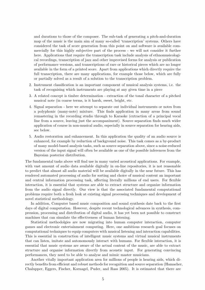
and durations to those of the composer. The sub-task of generating a pitch-and-durationmap of the music is the main aim of many so-called ‘transcription’ systems. Others haveconsidered the task of score generation from this point on and software is available com-mercially for this highly subjective part of the process - we will not consider it furtherhere. Applications that require the transcription task include analysis of ethnomusicologi-cal recordings, transcription of jazz and other improvised forms for analysis or publicationof performance versions, and transcriptions of rare or historical pieces which are no longeravailable in the form of a printed score. Apart from applications which directly require thefull transcription, there are many applications, for example those below, which are fullyor partially solved as a result of a solution to the transcription problem.

2. Instrument classification is an important component of musical analysis systems, i.e. thetask of recognising which instruments are playing at any given time in a piece

3. A related concept is timbre determination - extraction of the tonal character of a pitchedmusical note (in coarse terms, is it harsh, sweet, bright, etc.

4. Signal separation - here we attempt to separate out individual instruments or notes froma polyphonic (many-note) mixture. This finds application in many areas from soundremastering in the recording studio through to Karaoke (extraction of a principal vocalline from a source, leaving just the accompaniment). Source separation finds much widerapplication of course in non-musical audio, especially in source separation for hearing aids,see below.

5. Audio restoration and enhancement. In this application the quality of an audio source isenhanced, for example by reduction of background noise. This task comes as a by-productof many model-based analysis tasks, such as source separation above, since a noise-reducedversion of the input signal will often be available as one of the possible inferences from theBayesian posterior distribution.

The fundamental tasks above will find use in many varied acoustical applications. For example,with vast amount of audio data available digitally in on-line repositories, it is not reasonableto predict that almost all audio material will be available digitally in the near future. This hasrendered automated processing of audio for sorting and choice of musical content an importantand central information processing task, affecting literally millions of end users. For flexibleinteraction, it is essential that systems are able to extract structure and organize informationfrom the audio signal directly. Our view is that the associated fundamental computationalproblems require both a fresh look at existing signal processing techniques and development ofnovel statistical methodology.

In addition, Computer based music composition and sound synthesis date back to the firstdays of digital computation. However, despite recent technological advances in synthesis, com-pression, processing and distribution of digital audio, it has yet been not possible to constructmachines that can simulate the effectiveness of human listening.

Statistical methodolgies are now migrating into human computer interaction, computergames and electronic entertainment computing. Here, one ambitious research goal focuses oncomputational techniques to equip computers with musical listening and interaction capabilities.This is essential in construction of intelligent music systems and virtual musical instrumentsthat can listen, imitate and autonomously interact with humans. For flexible interaction, it isessential that music systems are aware of the actual content of the music, are able to extractstructure and organise information directly from acoustic input. For generating convincingperformances, they need to be able to analyse and mimic master musicians.

Another vitally important application area for millions of people is hearing aids, which di-rectly benefits from efficient and robust methods for recognition and source separation (Hamacher,Chalupper, Eggers, Fischer, Kornagel, Puder, and Rass 2005). It is estimated that there are

5

almost nine million hearing impaired people in the UK alone; a number which is believed to beincreasing with rapidly aging population. Progress in this field is likely to improve the qualityof life for a sizeable segment of society. Recently, modern hearing aids have evolved into pow-erful computational devices and with advances in wireless communications, it is becoming nowfeasible to delegate computation to external portable computing devices. This provides unprece-dented possibilities along with interesting computational challenges for online adaptation, sincein the next generation of hearing aids, it will be feasible to run sophisticated statistical signalprocessing and machine learning algorithms. Finally, computational audio processing finds ap-plication in the areas of monitoring, rescue and surveillance, computer aided music education,musicology, music perception and cognition research.

piano

time

ampl

itude

viola piccolo french horn cymbals congas

frame index

freq

uenc

y in

dex

Figure 4: Some acoustical instruments, examples of typical time series and corresponding spectro-grams (time varying magnitude spectra – modulus of short time Fourier transform) computed withFFT. (Audio data and images from RWCP Instrument samples database).

piano + piccolo + cymbals

Figure 5: Superposition. The time series and the magnitude spectrogram of the resulting signalwhen some of the instruments play concurrently.

6

2 Fundamental Audio Processing Tasks

From the above discussion of the challenges facing audio processing, some fundamental taskscan be identified for treatment by Bayesian techniques. Firstly, we can hope to address thesuperposition task in a model-based fashion, by posing models that capture the behaviour ofsuperimposed signals. These are similar in flavour to the latent factors analysed in some sta-tistical modelling problems. A generic model for observed data Y , under a linear superpositionassumption, will then be:

Y =

I∑

i=1

si (1)

where the si represent each of the I individual audio sources present. We pose this very basicmodel here as a single-channel observation model, although it is straightforward to extendthe model to the multi-channel case, in which case it will be usual to include also channel-specific mixing coefficients. The sources and data will typically be audio time series, but canalso represent expansion coefficients of the audio in some other domain such as the Fourier orwavelet domain, as will be made clear in context later. We may make the model a little moresophisticated by making the data a stochastic function of the sources, and in this case we willspecify some non-degenerate likelihood function p(Y |∑I

i=1 si).We typically assume that the individual sources si, one or more of which may be background

noise terms, are independent a priori. They are parameterised by θi, which represent informa-tion about the sound generation process for that particular source, including perhaps its pitchand other characteristics (number of partials, etc.), encoded through a conditional distributionand prior distribution for each source:

p(si, θi) = p(si|θi)p(θi)

Dependence between the θi, for example to model the harmonic relationships of notes within achord, can of course be included as desired when considering the joint distribution of sourcesand parameters. To this model we can add unknown hyperparameters Λ with prior p(Λ) in theusual way, and incorporate model uncertainty through an additional prior distribution on thenumber of components I. The specification of suitable source models p(si|θi) and p(θi), as wellas the form of likelihood function p(Y |∑I

i=1 si), will form a substantial part of the remainderof the paper.

Several fundamental inference tasks can then be identified from this generic model, includingthe source separation and polyphonic music transcription tasks identified above.

2.1 Source Separation

In source separation, the task is to infer the source signals si themselves, given the observedsignal Y . Collecting the sources together as S = {si}I

i=1 and the parameters as Θ = {θi}Ii=1,

the Bayesian formulation of the problem can be stated, under a fixed number of sources I, as(see for example (Mohammad-Djafari 1997; Knuth 1998; Rowe 2003; Fevotte and Godsill 2006;Cemgil, Godsill, and Fevotte 2007))

p(S|Y ) =1

P (Y )

∫

p(Y |S,Λ)p(S|Θ,Λ)p(Λ)p(Θ)dΛdΘ (2)

where, under our deterministic model above in Eq. 1 the likelihood function p(Y |S,Λ) will bedegenerate. The marginal likelihood P (Y ) plays a key role when model order uncertainty is tobe incorporated into the problem, for example when the number of sources N is unknown andneeds to be estimated (Miskin and Mackay 2001).

7

Additional considerations which may additionally be included in the above framework in-clude convolutive (filtered) and non-stationary mixing of the sources - both scenarios are ofpractical interest and still pose significant computational challenges. Once the posterior distri-bution is computed by evaluating the integral, point estimates of the sources can be obtainedusing suitable estimation criteria, such as marginal MAP or posterior mean estimation, al-though in the latter case one has to be especially careful with the interpretation of expectationsin models where likelihoods and priors are invariant to source permutations.

2.2 Polyphonic Music Transcription

Music transcription refers to extraction of a human readable and interpretable description froma recording of a music performance, see Fig. 6. In cases where more than a single musicalnote plays at a given time instant, we term this task polyphonic music transcription. Interestin this problem is largely motivated by a desire to implement a program to infer automaticallya musical notation, such as the traditional western music notation, listing the pitch valuesof notes, corresponding timestamps and other expressive information in a given performance.These quantities will be encoded in the above model through the parameters θi of each notepresent at a given time. Simple models will encode only the pitch of the note in θi, whilemore complex models can include expressive information, instrument-specific characteristicsand timbre, etc.

Apart from being an interesting modelling and computational problem in its own right,automated extraction of a score-like description is potentially very useful in a broad spectrumof applications such as interactive music performance systems, music information retrieval andmusicological analysis of musical performances, not to mention as an aid to the source separationtask identified above. However, in its most unconstrained form, i.e., when operating on anarbitrary acoustical input, music transcription remains a very challenging problem, owing tothe wide variation in acoustical conditions and characteristics of musical instruments. In spiteof these difficulties, a practical engineering solution is possible by careful incorporation of priorknowledge from cognitive science, musicology, musical acoustics, and by use of computationaltechniques from statistics and digital signal processing.

t/sec

f/Hz

0 1 2 3 4 5 6 7 80

1000

2000

3000

4000

5000

0

10

20

Figure 6: Polyphonic Music Transcription. The task is to generate a human readable score as shownbelow, given the acoustic input. The computational problem here is to infer pitch, number of notes,rhythm, tempo, meter, time signature. The inference can be achieved online (filtering) or offline(smoothing), depending upon requirements.

2.3 Hierarchical Models for Musical Audio

In a statistical sense, music transcription is an inference problem where, given a signal, wewant to find a score that is consistent with the encoded music. In this context, a score canbe contemplated as a collection of “musical objects” (e.g., note events) that are rendered by aperformer to generate the observed signal. The term “musical object” comes directly from ananalogy to visual scene analysis where a scene is “explained” by a list of objects along with a

8

Score Expression

Piano-Roll

Signal

Figure 7: A hierarchical generative model for music transcription. In this model, an unknown scoreis rendered by a performer into a piano-roll. The performer introduces expressive timing deviationsand tempo fluctuations. The piano-roll is rendered into audio by a synthesis model. The piano rollcan be viewed as a symbolic representation, analogous to a sequence of MIDI events. Given theobservations, transcription can be viewed as Bayesian inference of the score. Somewhat simplified,the techniques described in this article can be viewed as inference techniques as applied to subgraphsof this graphical model.

description of their intrinsic properties such as shape, color or relative position. We view musictranscription from the same perspective, where we want to “explain” individual samples of amusic signal in terms of a collection of musical objects where each object has a set of intrinsicproperties such as pitch, tempo, loudness, duration or score position. It is in this respect thata score is a high level description of music.

Musical signals have a very rich temporal structure, and it is natural to think of them as beingorganized in a hierarchical way. At the highest level of this organization, which we may call as thecognitive (symbolic) level, we have a score of the piece, as, for instance, intended by a composer2.The performers add their interpretation to music and render the score into a collection of“control signals”. Further down on the physical level, the control signals trigger various musicalinstruments that synthesize the actual sound signal. We illustrate these generative processesusing a hierarchical graphical model (See Figure 7), where the arcs represent generative links.

This architecture is of course anything but new, and in fact underlies any music generatingcomputer program such as a sequencer. The main difference of our model from a conventionalsequencer is that the links are probabilistic, instead of deterministic. We use the sequenceranalogy in describing a realistic generative process for a large class of music signals.

In describing music, we are usually interested in a symbolic representation and not so muchin the “details” of the actual waveform. To abstract away from the signal details, we definean intermediate layer, that represents the control signals. This layer, that we call a “piano-roll”, forms the interface between a symbolic process and the actual signal process. Roughly,the symbolic process describes how a piece is composed and performed. Conditioned on thepiano-roll, the signal process describes how the actual waveform is synthesized. Conceptually,the transcription task is then to “invert” this generative model and recover back the originalscore. As an intermediate and less sophisticated task, we may try and invert back only as faras the piano-roll.

2In reality the music may be improvised and there may be actually not a written score. In this case we replacethe generative model with the intentions of the performer, which can still be expressed in our framework as a ‘virtual’musical score

9

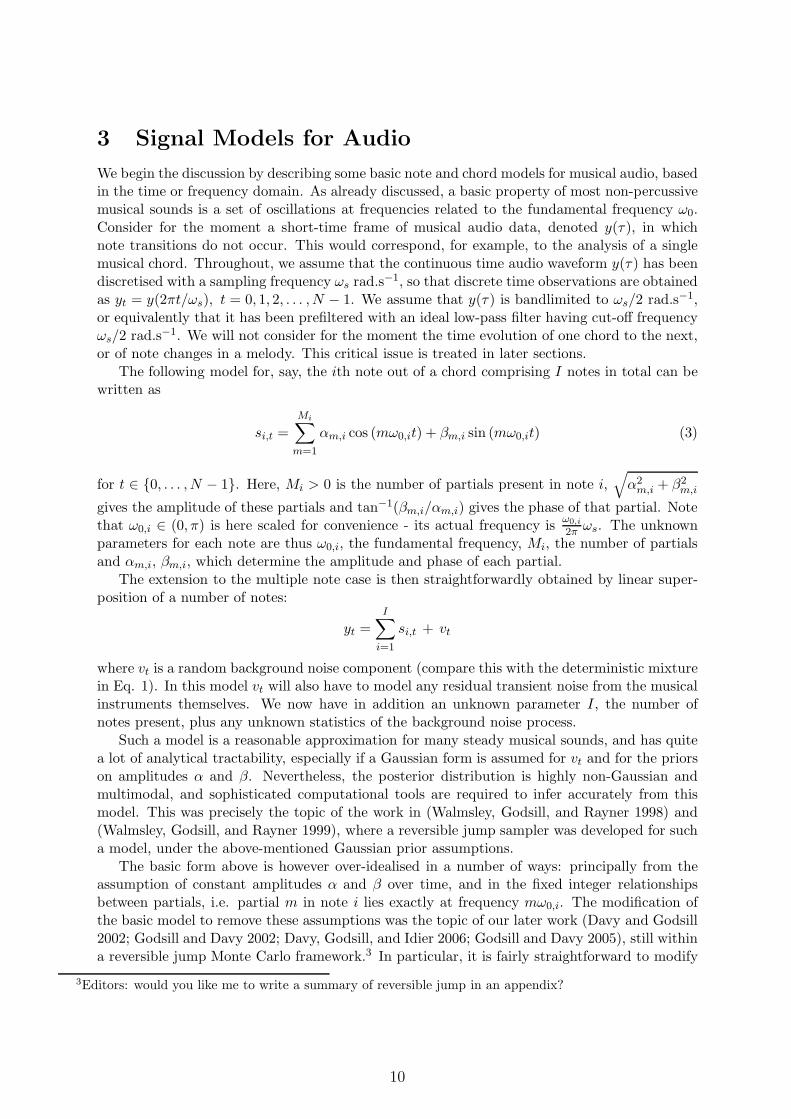
3 Signal Models for Audio

We begin the discussion by describing some basic note and chord models for musical audio, basedin the time or frequency domain. As already discussed, a basic property of most non-percussivemusical sounds is a set of oscillations at frequencies related to the fundamental frequency ω0.Consider for the moment a short-time frame of musical audio data, denoted y(τ), in whichnote transitions do not occur. This would correspond, for example, to the analysis of a singlemusical chord. Throughout, we assume that the continuous time audio waveform y(τ) has beendiscretised with a sampling frequency ωs rad.s−1, so that discrete time observations are obtainedas yt = y(2πt/ωs), t = 0, 1, 2, . . . , N − 1. We assume that y(τ) is bandlimited to ωs/2 rad.s−1,or equivalently that it has been prefiltered with an ideal low-pass filter having cut-off frequencyωs/2 rad.s−1. We will not consider for the moment the time evolution of one chord to the next,or of note changes in a melody. This critical issue is treated in later sections.

The following model for, say, the ith note out of a chord comprising I notes in total can bewritten as

si,t =

Mi∑

m=1

αm,i cos (mω0,it) + βm,i sin (mω0,it) (3)

for t ∈ {0, . . . , N − 1}. Here, Mi > 0 is the number of partials present in note i,√

α2m,i + β2

m,i

gives the amplitude of these partials and tan−1(βm,i/αm,i) gives the phase of that partial. Notethat ω0,i ∈ (0, π) is here scaled for convenience - its actual frequency is

ω0,i

2π ωs. The unknownparameters for each note are thus ω0,i, the fundamental frequency, Mi, the number of partialsand αm,i, βm,i, which determine the amplitude and phase of each partial.

The extension to the multiple note case is then straightforwardly obtained by linear super-position of a number of notes:

yt =

I∑

i=1

si,t + vt

where vt is a random background noise component (compare this with the deterministic mixturein Eq. 1). In this model vt will also have to model any residual transient noise from the musicalinstruments themselves. We now have in addition an unknown parameter I, the number ofnotes present, plus any unknown statistics of the background noise process.

Such a model is a reasonable approximation for many steady musical sounds, and has quitea lot of analytical tractability, especially if a Gaussian form is assumed for vt and for the priorson amplitudes α and β. Nevertheless, the posterior distribution is highly non-Gaussian andmultimodal, and sophisticated computational tools are required to infer accurately from thismodel. This was precisely the topic of the work in (Walmsley, Godsill, and Rayner 1998) and(Walmsley, Godsill, and Rayner 1999), where a reversible jump sampler was developed for sucha model, under the above-mentioned Gaussian prior assumptions.

The basic form above is however over-idealised in a number of ways: principally from theassumption of constant amplitudes α and β over time, and in the fixed integer relationshipsbetween partials, i.e. partial m in note i lies exactly at frequency mω0,i. The modification ofthe basic model to remove these assumptions was the topic of our later work (Davy and Godsill2002; Godsill and Davy 2002; Davy, Godsill, and Idier 2006; Godsill and Davy 2005), still withina reversible jump Monte Carlo framework.3 In particular, it is fairly straightforward to modify

3Editors: would you like me to write a summary of reversible jump in an appendix?

10

0 500 1000 1500 2000 2500 3000 3500 40000

0.1

0.2

0.3

0.4

0.5

0.6

0.7

0.8

0.9

1

Time index, t

ψ1,t

ψ2,t

ψ3,tψ

1,tψ

9,t....

Figure 8: Basis functions ψi,t, I = 9, 50% overlapped hanning windows.

the model so that the partial amplitudes α and β vary with time,

si,t =

Mi∑

m=1

αm,i,t cos (mω0,it) + βm,i,t sin (mω0,it) (4)

and we typically expand αm,i,t and βm,i,t on a finite set of smooth basis functions ψi,t withexpansion coefficients ai and bi:

αm,i,t =J∑

j=1

aiψi,t, βm,i,t =J∑

j=1

biψi,t

In our work we have adopted 50%-overlapped Hamming windows for the basis functions, seeFig. 8, with support either chosen a priori by the user or treated as a Bayesian random variable(Godsill and Davy 2005).

Alternative more general representations allow a fully stochastic variation of αm,i,t in thestate-space formulation, see section ??.

Further idealisations in these models include the assumption of constant fundamental fre-quencies with time and the Gaussian prior and noise assumptions, but in principle all can beaddressed in a principled Bayesian fashion.

3.1 A prior distribution for musical notes

Under the above basic time-domain model we need to assign prior distributions over the un-known parameters for a single note in the mix, currently {ω0,i,Mi,αi,βi}, where αi,βi arethe vectors of parameters αm,i,βm,i, m = 1, 2, ...,Mi. Under an assumed note system suchas an equally-tempered Western note system, we can augment this with a note number indexni. A suitable scheme is the MIDI note numbering system4 which labels middle C (or ‘C4’)as note number 60, and all other notes as integers relative to this - the A below this would

4See for example www.harmony-central.com/MIDI/doc/table2

11

−8 −6 −4 −2 0 2 4 6 80

0.2

0.4

0.6

0.8

1

1.2

1.4

log( ω0,i

), in semitones relative to A440Hz

Prio

r pr

obab

ility

den

sity

Figure 9: Prior for fundamental frequency p(ω0,i)

be 57, for example, and the A above middle C (usually at 440Hz in modern Western tuningsystems) would be note number 69. Other non-Western systems could also be encoded withinvariants of such a scheme. The fundamental frequency would then be expected to lie ‘close’to the expected frequency for a particular note number, allowing for performance and tuningdeviations from the ideal. Thus a prior for the observed fundamental frequency ω0,i can beconstructed fairly straightforwardly. We adopt here a truncated log-normal distribution for thenote’s fundamental frequency:

p(log(ω0,i)|ni) ∝{

N (µ(ni), σ2ω), log(ω0,i) ∈ [(µ(ni − 1) + µ(ni))/2, (µ(ni) + µ(ni + 1))/2)

0, otherwise

where µ(n) computes the expected log-frequency of note number n, i.e., when we are dealingwith A440 music in the equally tempered western system,

µ(n) = (n− 69)/12 log(2) + log(440/ωs) (5)

where once again ωsrad.s−1 is the sampling frequency of the data. Assuming p(n) is uniform fornow, the resulting prior p(ω0,i) is plotted in Fig. 9, capturing the expected clustering of notefrequencies at semitone spacings relative to A440.

The prior model for a note is completed with two components. Firstly a prior for thenumber of partials, p(Mi|ω0,i), is specified as uniform over the range {Mmin, ...,Mmax}, withlimits truncated to prevent partials at frequencies greater than ωs/2, the Nyquist rate. Secondlya prior for the amplitude parameters αi,βi must be specified. This turns out to be quite crucialto the modelling performance and here we initially proposed a Gaussian form. It is expectedhowever that partials at high frequencies will have lower energy than those at high frequencies,generally following a low-pass filter shape in the frequency domain. Coefficents αm,i and βm,i arethen assigned independent Gaussian prior distributions such that their amplitudes are assumed

12

100

101

10−10

10−9

10−8

10−7

10−6

10−5

10−4

10−3

10−2

10−1

100

Partial number, m

increasing ν

Figure 10: Family of km curves (log-log plot), T = 5, ν = 1, ..., 10.

to decay with increasing frequency of the partial number m. The general form of this is

p(αm,i, βm,i) = N (βm,i|0, g2i km)N (αm,i|0, g2

i km)

Here gi is a scaling factor common to all partials in a note and km is a frequency-dependentscaling factor to allow for the expected decay with increasing frequency for partial amplitudes.Following (Godsill and Davy 2005) the amplitudes are assumed to decay as follows:

km = 1/(1 + (Tm)ν)

where ν is a decay constant and T determines the cut-off frequency. Such a model is basedon empirical observations of the partial amplitudes in many real instrument recordings, andessentially just encodes a low pass filter with unknown cut-off frequency and decay rate. See forexample the family of curves with T = 5, ν = 1, 2, ..., 10, Fig. 10. It is worth pointing out thatthis model does not impose very stringent constraints on the precise amplitude of the partials:the Gaussian distribution will allow for significant departures from the km = 1/(1 + (Tm)ν)rule, as dictated by the data, but it does impose a generally low-pass shape to the harmonicsacross frequency. It is possible to keep these parameters as unknowns in the MCMC scheme (see(Godsill and Davy 2005)), although in the examples presented here we fix these to appropriatelychosen values for the sake of computational simplicity. gi, which can be regarded as the overall‘volume’ parameter for a note, is treated as an additional random variable, assigned an invertedGamma distribution for its prior. The Gaussian prior structure outlined here for the α and βparameters is readily extended to the time-varying amplitude case of Eq. (4), in which casesimilar Gaussian priors are applied directly to the expansion coefficients a and b, see (Davy,Godsill, and Idier 2006).

In the simplest case, a polyphonic model is then built by taking an independent prior over

13

0 2000 4000 6000 8000 10000 12000 14000 16000−0.5

0

0.5Waveform − slow release

0 2000 4000 6000 8000 10000 12000 14000 16000−0.5

0

0.5Waveform − fast release

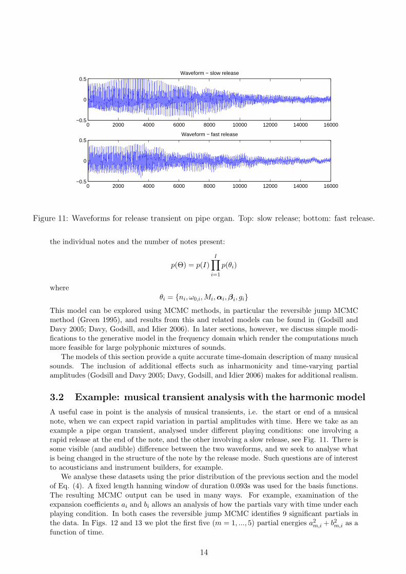
Figure 11: Waveforms for release transient on pipe organ. Top: slow release; bottom: fast release.

the individual notes and the number of notes present:

p(Θ) = p(I)

I∏

i=1

p(θi)

whereθi = {ni, ω0,i,Mi,αi,βi, gi}

This model can be explored using MCMC methods, in particular the reversible jump MCMCmethod (Green 1995), and results from this and related models can be found in (Godsill andDavy 2005; Davy, Godsill, and Idier 2006). In later sections, however, we discuss simple modi-fications to the generative model in the frequency domain which render the computations muchmore feasible for large polyphonic mixtures of sounds.

The models of this section provide a quite accurate time-domain description of many musicalsounds. The inclusion of additional effects such as inharmonicity and time-varying partialamplitudes (Godsill and Davy 2005; Davy, Godsill, and Idier 2006) makes for additional realism.

3.2 Example: musical transient analysis with the harmonic model

A useful case in point is the analysis of musical transients, i.e. the start or end of a musicalnote, when we can expect rapid variation in partial amplitudes with time. Here we take as anexample a pipe organ transient, analysed under different playing conditions: one involving arapid release at the end of the note, and the other involving a slow release, see Fig. 11. There issome visible (and audible) difference between the two waveforms, and we seek to analyse whatis being changed in the structure of the note by the release mode. Such questions are of interestto acousticians and instrument builders, for example.

We analyse these datasets using the prior distribution of the previous section and the modelof Eq. (4). A fixed length hanning window of duration 0.093s was used for the basis functions.The resulting MCMC output can be used in many ways. For example, examination of theexpansion coefficients ai and bi allows an analysis of how the partials vary with time under eachplaying condition. In both cases the reversible jump MCMC identifies 9 significant partials inthe data. In Figs. 12 and 13 we plot the first five (m = 1, ..., 5) partial energies a2

m,i + b2m,i as afunction of time.

14

0 10 20 30 40 50 60 70 80 900

0.02

0.04

m=

1

Pipe organ − slow release

0 10 20 30 40 50 60 70 80 900

0.02

0.04

m=

2

0 10 20 30 40 50 60 70 80 900

0.02

0.04

m=

3

0 10 20 30 40 50 60 70 80 900

0.02

0.04

m=

4

0 10 20 30 40 50 60 70 80 900

0.02

0.04

Expansion Coefficient i

m=

5

Figure 12: Magnitudes of partials with time: slow release.

0 10 20 30 40 50 60 70 80 900

0.020.04

m=

1

Pipe organ − fast release

0 10 20 30 40 50 60 70 80 900

0.020.04

m=

2

0 10 20 30 40 50 60 70 80 900

0.020.04

m=

3

0 10 20 30 40 50 60 70 80 900

0.020.04

m=

4

0 10 20 30 40 50 60 70 80 900

0.020.04

Expansion coefficient i

m=

5

Figure 13: Magnitudes of partials with time: fast release.

15

Examining the behaviour from the MCMC output we can see that the third partial is sub-stantially elevated during the slow release mode, between coefficients i = 30 to 40. Also, in theslow release mode, the fundamental frequency (m = 1) decays at a much later stage relative to,say, the fifth partial, which itself decays more slowly in that mode. One can also use the modeloutput to perform signal modification; for example time stretching or pitch shifting of the tran-sient are readily achieved by reconstructing the signal using the MCMC-estimated parametersbut modifying the hanning window basis function length (for time-stretching) or reconstructingwith modified fundamental frequency ω0, see www-sigproc.eng.cam.ac.uk/~sjg/haba. Thedetails of our reversible jump MCMC scheme are quite complex, involving a combination ofspecially designed independence Metropolis-Hastings proposals and random walk-style propos-als for the note frequency variables. In the frequency-domain models described in section 5 weuse essentially the same MCMC scheme, with simpler likelihood functions - some more detailsof the proposals used are given there.

4 Dynamical State Space Models

The models introduced in the previous section are generalised linear models, where the expan-sion coefficients ai and bi are assumed to be a-priori independent across frames. While thesemodels are quite useful, they are not very realistic models of the underlying physics, as audiois essentially the result of unfolding dynamical processes. It is possible to introduce randomwalk dynamics on the expansion coefficients. In contrast, we will describe the evolution of theexpansion coefficients in state space form, via state space models. Such representations can bederived from well known sinusoidal signal representations such described in the appendix A andare one step towards physical models.

The audio signal can be written as a sum of exponentially decaying or windowed sinusoids(See Eq. (3) or examples in appendix sections A.2 and A.3). However, richer processes with morecomplex behaviour can be described by state space models. This involves defining stochasticsignal representations and higher level, unobserved stochastic elements, such as change pointprocesses and model-order indicators, which are combined to form hierarchical Bayesian models.The reader will notice that these models exhibit a variety of structures that arise from theinteraction between the low-level signal models and the high-level latent processes. We alsodescribe associated inference tasks and efficient methods for their solution which take advantageof the model structures.

4.1 Conditionally Linear Dynamical Systems with regime switch-

ing

We start this section with a general framework to highlight and unify the basic modellingideas. Our goal is to construct a model that can mimic the qualitative behaviour of acousticalsystems (such as musical instruments shown in figure 4) yet still has some analytical structurewhich allows efficient inference. Our starting point is the conditionally-linear state space model.This is motivated by the fact that the harmonic structure of audio signals, arising the physicalprocesses by which they are generated, can conveniently be formulated in state-space form.

Here, we construct a generic model as a cascade of two systems with an excitation (e.g., vi-brating string) feeding into a resonator (e.g., the body of an acoustic instrument). Respectively,

16

Figure 14: A damped oscillator in state space form.

se and sf are the states of the excitation system and the resonating system:

sek ∼ N

(

sek;Aks

ek−1, Qk

)

sfk = Afts

fk−1 +Bfts

ek

yk ∼ N(

yk;Csfk, R

)

(6)

where C is an observation matrix and R is the observation noise. This model is, of course, aparticular parametrisation of the general linear dynamical system. The main idea, in the generalsense, is to define a nonstationary process with p(A, Q) over the sequence of transition matricesA ≡ {Ak}k≥0 and the transition noise covariances Q ≡ {Qk}k≥0. The posterior estimatesof these latent parameters, when integrated over latent states sk will describe the signal in acompact way. There are clearly many possibilities in defining prior distributions over A and Q.In the sequel, we will define several realistic models in this framework.

We define a sequence of discrete switch variables r = r0:K−1 and draw the state matricesconditionally. Here this indicators r are abstract, but in practice will correspond to onsets,offsets or note labels, depending upon the context of the task at hand.

p(r) = p(r0:K−1) = p(r0)

K−1∏

k=1

p(rk|rk−1)

Ak ∼ p(Ak|rk) Qk ∼ p(Qk|rk)

This includes the special cases such as when Ak = A(r), i.e. a deterministic function of r (withthe choice p(Ak|r) = δ(Ak −A(r))), similar with Qk.

In principle, one could work with in any state space coordinate system by appropriatelychoosing the state matrices. However, we prefer to work in a representation to maintain theinterpretability of the parameters. This representation is closely related to the sinusoidal modelsand described in detail in the appendixA.

4.1.1 Dynamic Harmonic model

To highlight our specific construction, we start this section with an example. We consider asecond order oscillator systems, driving a second order resonator, following Eq.(6). We specifythe models by a specific choice of transition matrices and transition noise covariance

Ak = Z(γk, ωk) Aft = Z(γft, ωft) Qk = qkI

where

Z(γ, ω) ≡ e−Lγν

(

cos(Lων) − sin(Lων)sin(Lων) cos(Lων)

)⊤

We have a L×L observation noise covariance matrix R, and an L× 2K observation matrixC, where each column is a damped sinusoidal (see Eq.(32) in the appendix). For simplicity,we consider the case when frame length is L = 1, where we generate the signal sample by

17

sample. See Fig.14. Note that in this representation the state vector s is simply the expansioncoefficients (real amplitudes) a and b, introduced in the previous section.

The transition matrix Ak generates a damped sinusoidal which is fed into the system withtransition matrix Aft via the 2 × 2 input matrix Bft, here taken as Bft = I. The driving noiseof the excitation has time dependent variance Qk = qkI. The observation matrix in this caseis C =

(

1 0)

. The discrete variables rk in this model encode onsets and offsets. We definea Markov chain rk for k = 0, 1, . . . , where rk ∈ {on = 1, off = 0}, with the state transitiondistribution parametrised as p(rk = on|rk−1 = on) = πon and p(rk = off|rk−1 = off) = πoff.Conditioned on rk and rk−1, we let

qk =

qonset if rk = on and rk−1 = offqon if rk = on and rk−1 = on0 otherwise

γk =

{

γon if rk = onγoff if rk = off

The hyper parameters of this model are the prior state probabilities πon and πoff transitionvariances qonset, qon, the excitation model transition damping constants γon, γoff and frequencyωex, the resonator parameters γft and ωft and the observation noise variance R. With eachnew onset event (rk−1,k = (off, on))), the excitation state is reinitialised from a Gaussian withvariance qonset and driven with noise until the next onset time.

Even this rather simple model displays quite rich behaviour, as shown by typical realisationsin Fig. 4.1.1. Given the observed signals, posterior inference for latent variables gives structuralinformation about the signal. For example, E(ωk|y1:k) will give an online estimate of the instan-taneous frequency of the excitation and the posterior transition variance estimate E(rk|y1:K)will give an indication of onsets and offsets.

4.2 Dynamic Harmonic model and Changepoint models

As previously discussed, acoustic systems, and in particular pitched musical instruments tendto create oscillations with modes at frequencies that are roughly related by ratios of integers(Fletcher and Rossing 1998). The fundamental frequency, corresponding the largest commondivisor of mode frequencies, is strongly correlated with the perceived pitch in music. For tran-scription, we need to estimate the fundamental frequency as well as the onsets and offsets tomark the beginning and the end of each note. This problem can be formalised using the har-monic models introduced in section 3, coupled to a change-point structure related to the mixturemodel of the previous section. We now combine a number of oscillators that are harmonicallyrelated by a fundamental frequency. We define the block diagonal state evolution matrix

Ak = diag(Z0,k, . . . , Zν,k, . . . ZW−1,k)

with possible choices

Zν,k = Z(γk, ωk)ν = Z(νγk, νωk)

ν (7)

Here, the power ν adjust both the damping and the frequency. This ensures that all oscillatorsare tuned to a multiple of a base fundamental frequency.

Both γ and ω can assume positive real values and the exact posterior has a complicatedform due to the nonlinear relationship with observed data. One simplification, in contrast withmodels introduced earlier in section 3, is choosing the fundamental frequencies from a finite settaking values on a prespecified grid such as the tempered scale or finer gradatation accordingto the desired frequency resolution,

ωk = ω(mk) mk ∈ 1 . . .M

18

k(a) Only periodic excitation

e kr k

y k

γon = 5 · 10−4 γoff = 0.03 qon = 0

k(b) Periodic + noise excitation

e kr k

y k

γon = 0.01 γoff = 0.1 qon = 1

k(c) Only noise excitation

e kr k

y k

γon = 1 γoff = 1 qon = 1

k(d) Only impulsive excitation

e kr k

y k

γon = 1 γoff = 1 qon = 0

Figure 15: Time series yk generated by a cascade of two phasors in Eq.6 (middle), conditioned on theindicator sequence r0:K−1, (top – black = on,white = off ). The excitation signals are shown at thebottom ek = (1 0) sk. The other hyperparameters are fixed at γft = 0.005, ωft = π/15, ωex = π/16,qonset = 1

19

Here, m is a discrete index variable and ω(m) is a function to the associated fundamentalfrequency. For example, when m corresponds to the pitch label; ω(m) corresponds to thefundamental frequency, as in (5) for example. We define the following pair of discrete latentvariables

dk = (rk,mk)

and obtain a discrete chain that can visit one of the |d| = 2M states at each time slice k. Theprior can be taken Markovian as p(dk|dk−1). The most likely onsets, offsets and the funda-mental frequency can be inferred via calculating the marginal maximum a-posteriori (MMAP)trajectory

d∗0:K−1 = arg maxd0:K−1

∫

p(y0:K−1|s0:K−1)p(s0:K−1|d0:K−1)p(d0:K−1)ds0:K−1

Alternatively, when online estimates are required, as is the case in real-time interaction, thefiltering density can be computed recursively

p(sk, dk|y0:k) ∝∑

dk−1

∫

p(yk|sk)p(sk, dk|sk−1, dk−1)p(sk−1, dk−1|y0:k−1)dsk−1

p(dk|y0:k) =

∫

p(sk, dk|y0:k)dsk

For general switching state space models, exact inference of the above quantities is not tractable.Whilst in principle the filtering distribution can be represented exactly as a Gaussian mixtureand propagated in closed form, we have to still resort to approximations since the numberof mixture components needed for exact representation of p(sk, dk|y0:k) increases exponentiallywith increasing k. However, there is an interesting special case, when condtioned on a particularconfiguration of d, there is a “forgetting” property, i.e., if

p(sk|dk−1:k = d, sk−1) = p(sk|dk−1:k = d)

In this case, the exact MMAP trajectory or the filtering density (Fearnhead 2003; Cemgil, Kap-pen, and Barber 2004) can be computed in polynomial time. This can be shown by considering

all trajectories d(j)0:k for j = 1 . . . |d|k+1 of the discrete states d upto time k. One can show

that trajectories (j′) which are dominated by (j) in terms of conditional marginal likelihood

z(j′) ≤ z(j) ≡ p(y0:k, r(j)0:k) can be discarded without destroying optimality. This greedy pruning

strategy is optimal and leaves only a number of trajectories that is increasing polynomially withtime (Cemgil, Kappen, and Barber 2004).

4.3 Polyphony and factorial models

The models described so far are useful for modelling complex sound sources. Yet, extensions arerequired for source separation or polyphonic transcription. This is typically done via factorialmodels, i.e., by constructing models over the product spaces of the individual sources, as wasdone for the static case in section 3, eq. (3).

One possible construction assumes that the audio is a superposition of several sources,indexed via i = 1 . . . I, with each source i modelled using the same model class, yet with differenthyperparameter instantiations. Here, we first consider a factorial switching state space modelfor music transcription. Here, each latent process ν = 1 . . . W corresponds to a “piano key”.Indicators d0:W−1,0:K−1 encode a latent piano roll. Given this model, polyphonic transcriptioncan be obtained as

d∗0:W−1,0:K−1 = argmaxd

∫

p(y|s)p(s|d)p(d)ds

20

d0 · · · dk · · · dK−1

Qν0 · · · Qν

k · · · QνK−1

Aν0 · · · Aν

k · · · AνK−1

sν0 · · · sν

k · · · sνK−1

ν = 0 . . . W − 1

y0 yk yK−1

500 1000 1500 2000 2500 3000 3500

Figure 16: (Left) Switching state space model with a block diagonal state transition matrix whereeach block is denoted by ν. The dynamic harmonic model corresponds to the case when the blocksof the transition matrix are chosen as Ak = Z(γk, ωk). (Right) Pitch detection and onset selectionof a signal recorded from a bass guitar. The MMAP state trajectory is show as rk = on = black andthe vertical axis denotes the pitch label index mk.

di,0 · · · di,k · · · di,K−1

Qνi,0 · · · Qν

i,k · · · Qνi,K−1

Aνi,0 · · · Aν

i,k · · · Aνi,K−1

sνi,0 · · · sν

i,k · · · sνi,K−1

ν = 0 . . . W − 1

i = 1 . . . I

y0 yk yK−1

i

k

y kν

Figure 17: A Factorial Switching state space model and typical realisations. The task of polyphonictranscription is to find the maximum marginal a-poteriori estimate of the latent switches d∗ givenobservations

21

A factorial switching state space model for polyphonic transcription is introduced in (Cemgil,Kappen, and Barber 2004) and some further strategies have been investigated in (Cemgil 2007).The model and a typical realisation is shown in Fig. 17. However, efficient inference in factorialswitching state space models is still an open problem. In the presence of a large number ofconcurrent sources I, even a single time slice is intractable as the discrete variables in theproduct space have a cardinality that scales exponentially as O(|d|I). Even conditioned on d,the latent continuous state dimension |s| can be very large for realistic models. and analyticalintegration over s via Kalman filtering techniques is computationally heavy. The main reasonfor this bottleneck in inference is the coupling between states s. When these are integratedout, all time slices of the discrete indicators become coupled and the exact inference problemis reduced to an intractable combinatorial optimisation problem. In the sequel, we will discussmodels where the couplings are ignored.

5 Frequency domain models

The previous two sections described various time domain models for musical audio, includingsinusoidal models and state-space models. The models are quite accurate for many examples ofaudio, although they show some non-robust properties in the case of signals which are far fromsteady-state oscillation and for instruments which do not closely obey the laws described above.Perhaps more critically, for large polyphonic mixes of many notes, each having potentially manypartials, the computations can become very expensive, in particular the calculation of marginallikelihood terms in the presence of many Gaussian components αi and βi. Computing themarginal likelihood is costly as this requires computation of Kalman filtering equations for alarge state space (that scales with the number of tracked harmonics) and for very long timeseries (as typical audio signals are sampled at 44.1 KHz). Hence, either efficient approximationsneed to be developed or simplified models need to be constructed.

In this section we at least partially bypass the computational issues by working with approx-imate models in the frequency domain. These allow for direct likelihood calculations withoutresorting to expensive matrix inversions and determinant calculations. Later in the chapter thesemodels will be elaborated further to give sophisitcated Bayesian non-negative matrix factorisa-tion algorithms which are capable of learning the structure of the audio events in a semi-blindfashion. Here initially, though, we work with simple model-based structures in the frequencydomain that are analogous to the time domain priors of the section 3. There are several routes toa frequency domain representation, including multi-resolution transforms, wavelets, etc., thoughhere we use a simple windowed discrete Fourier transform as examplar. We now propose twoversions of a frequency domain likelihood model, both of which bypass the main computationalburden of the high-dimensional time-domain Gaussian models.

5.0.1 Gaussian frequency-domain model

The first model proposed is once again a Gaussian model. In the frequency domain we willhave typically complex-valued expansion coefficients of the data on a one-dimensional lattice offrequency values ν ∈ N , i.e. a set of spectrum values yν . The assumption is that the contributionof each musical source term to the expansion coefficients is as independent zero-mean (complex)Gaussians, with variance determined by the parameters of the musical note:

si,ν ∼ NC(0, λν(θi))

where θi = {ni, ω0,i,Mi, gi} has the same interpretation as for the earlier time-domain model,but now we can neglect the α and β coefficients since the random behaviour is now directly

22

0.2 0.4 0.6 0.8 1 1.2 1.40

10

20

30

40

50

Normalised frequency

Figure 18: Template function λν(θi) with Mi = 8, ω0,i = 0.71, Gaussian pulse shape.

modelled by si,ν . This is a very natural formulation for generation of polyphonic models sincewe can add a number of sources together to make a single complex Gaussian data model:

yν ∼ NC(0, Sv,ν +

I∑

i=1

λν(θi))

Here, Sv,ν > 0 models a Gaussian background noise component in a manner analogous tothe time-domain formulation’s vt and it then remains to design the positive-valued ‘template’functions λ. Once again, Fig. 1.1 gives some guidance as to the general characteristics required.We then model the template using a sum of positive valued pulse waveforms φν , shifted to becentred at the expected partial position, and whose amplitude decays with increasing partialnumber:

λν(θi) =

Mi∑

m=1

g2i kmφν−mω0,i

(8)

where km, gi and Mi have exactly the same interpretation as in the time-domain model. Anexample template construction is shown in Fig. 18, in which a Gaussian pulse shape has beenutilised.

5.0.2 Point process frequency-domain model

The Gaussian frequency domain model requires a knowledge of the conditional distribution forthe whole range of spectrum values. However, the salient features in terms of pitch estimationappear to be the peaks of the spectrum see Fig. 1.1. Hence a more parsimonious likelihoodmodel might work only with the peaks detected from the Fourier magnitude spectrum. Thus wepropose as an alternative to the Gaussian spectral model, a point process model for the peaks inthe spectrum. Specifically, if the peaks in the spectrum of an individual note are assumed to bedrawn from a one-dimensional inhomogeneous Poisson point process having intensity functionλν(θi) (considered as a function of continuous frequency ν), then the combined set of peaksfrom many notes may be combined, under an independence assumption, to give a Poisson pointprocess whose intensity function is the sum of the individual intensities (Grimmett and Stirzaker2001). Suppose we detect a set of peaks in the magnitude spectrum {pj}J

j=1, νmin < pj < νmax.

23

0 500 1000 1500 2000 2500 3000 3500 4000 4500−0.2

−0.15

−0.1

−0.05

0

0.05

0.1

0.15

0.2

time (samples)

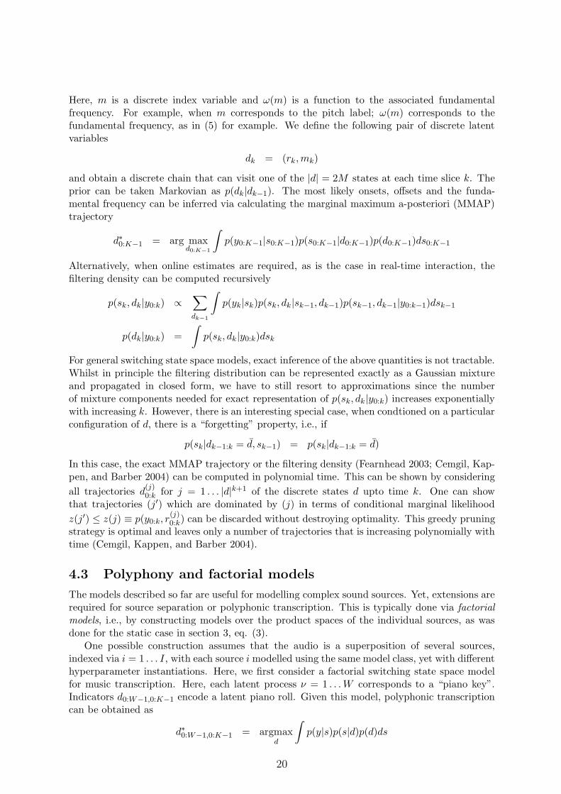
yt

Figure 19: Audio waveform - single chord data.

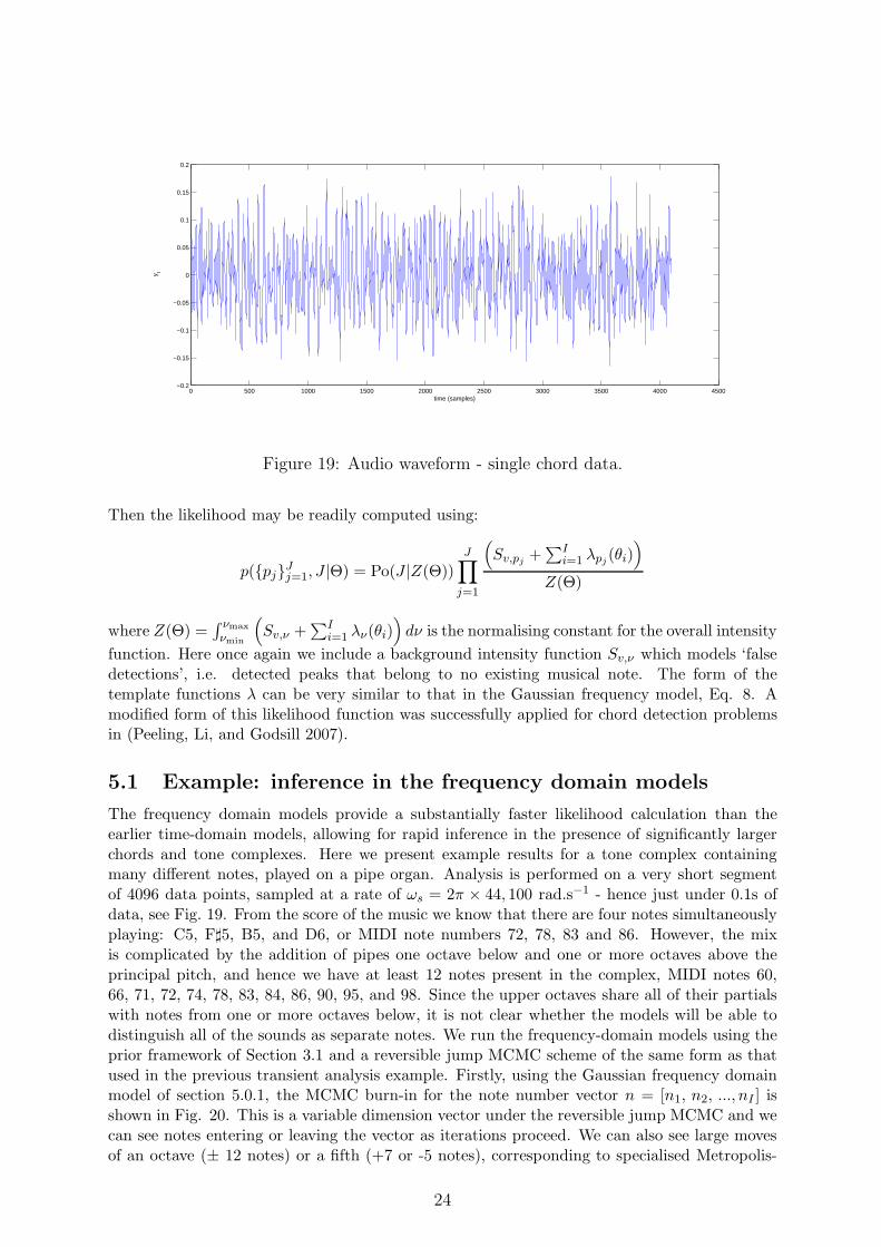
Then the likelihood may be readily computed using:

p({pj}Jj=1, J |Θ) = Po(J |Z(Θ))

J∏

j=1

(

Sv,pj+∑I

i=1 λpj(θi))

Z(Θ)

where Z(Θ) =∫ νmax

νmin

(

Sv,ν +∑I

i=1 λν(θi))

dν is the normalising constant for the overall intensity

function. Here once again we include a background intensity function Sv,ν which models ‘falsedetections’, i.e. detected peaks that belong to no existing musical note. The form of thetemplate functions λ can be very similar to that in the Gaussian frequency model, Eq. 8. Amodified form of this likelihood function was successfully applied for chord detection problemsin (Peeling, Li, and Godsill 2007).

5.1 Example: inference in the frequency domain models

The frequency domain models provide a substantially faster likelihood calculation than theearlier time-domain models, allowing for rapid inference in the presence of significantly largerchords and tone complexes. Here we present example results for a tone complex containingmany different notes, played on a pipe organ. Analysis is performed on a very short segmentof 4096 data points, sampled at a rate of ωs = 2π × 44, 100 rad.s−1 - hence just under 0.1s ofdata, see Fig. 19. From the score of the music we know that there are four notes simultaneouslyplaying: C5, F♯5, B5, and D6, or MIDI note numbers 72, 78, 83 and 86. However, the mixis complicated by the addition of pipes one octave below and one or more octaves above theprincipal pitch, and hence we have at least 12 notes present in the complex, MIDI notes 60,66, 71, 72, 74, 78, 83, 84, 86, 90, 95, and 98. Since the upper octaves share all of their partialswith notes from one or more octaves below, it is not clear whether the models will be able todistinguish all of the sounds as separate notes. We run the frequency-domain models using theprior framework of Section 3.1 and a reversible jump MCMC scheme of the same form as thatused in the previous transient analysis example. Firstly, using the Gaussian frequency domainmodel of section 5.0.1, the MCMC burn-in for the note number vector n = [n1, n2, ..., nI ] isshown in Fig. 20. This is a variable dimension vector under the reversible jump MCMC and wecan see notes entering or leaving the vector as iterations proceed. We can also see large movesof an octave (± 12 notes) or a fifth (+7 or -5 notes), corresponding to specialised Metropolis-

24

0 500 1000 1500 2000 2500 300050

60

70

80

90

100

110

MCMC Iteration No.

MID

I Not

e nu

mbe

r (M

iddl

e C

=60

)

Figure 20: Evolution of the note number vector with iteration number - single chord data. Gaussianfrequency domain model.

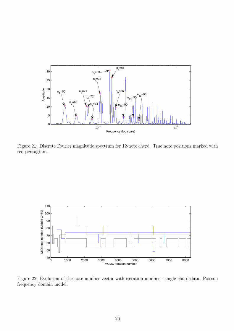
Hastings moves which center their proposals on the octave or fifth as well as the locality of thecurrent note. As is typical of these models, the MCMC becomes slow moving once convergedto a good mode of the distribution and further large moves only occur occasionally. There is agood case here for using adaptive or population MCMC schemes to improve the properties ofthe MCMC. Nevertheless, convergence is much faster than for the earlier proposed time domainmodels, particularly in terms of the model order sampling, which was here initialised at I = 1,i.e. one single note present at the start of the chain. Specialised independence proposals havealso been devised, based on simple pitch estimation methods applied to the raw data. Theseare largely responsible for the initiation of new notes in the MCMC chain. In this instancethe MCMC has identified correctly 7 out of the (at least) 12 possible pitches present in themusic: 60, 66, 71, 72, 74, 78, 86. The remaining 5 unidentified pitches share all of their partialswith lower pitches estimated by the algorithm, and hence it is reasonable that they remainunestimated. Examination of the discrete Fourier magnitude spectrum (Fig. 21) shows thatthe higher pitches (with the possible exception of n7 = 83, whose harmonics are modelled byn3 = 71) are generally buried at very low amplitude in the spectrum and can easily be absorbedinto the model for pitches one or more octaves lower in pitch.

We can compare these results with those obtained using the Poisson model of section 5.0.2.The MCMC was run under identical conditions to the Gaussian model and we plot the equivalentnote index output in Fig. 22. Here we see that fewer notes are estimated, since the basic pointprocess model takes no account of the amplitudes of the peaks in the spectrum, and hence ishappy to assign all harmonics to the lowest possible fundamental pitch. The four predominantpitches estimated are the four lowest fundamentals: 60, 66, 71 and 74. The sampler is, however,generally more mobile and we see a better and more rapid exploration of the posterior.

25

10−1

100

0

5

10

15

20

25

30

Frequency (log scale)

Am

plitu

de n1=60

n2=66

n3=71

n4=72

n12

=98n

11=95

n5=74 n

10=90

n9=86

n8=84

n6=78

n7=83

Figure 21: Discrete Fourier magnitude spectrum for 12-note chord. True note positions marked withred pentagram.

0 1000 2000 3000 4000 5000 6000 7000 800040

50

60

70

80

90

100

110

MCMC iteration number

MID

I not

e nu

mbe

r (M

iddl

e C

=60

)

Figure 22: Evolution of the note number vector with iteration number - single chord data. Poissonfrequency domain model.

26

5.2 Further prior structures for Transform domain representa-tions

In audio processing, the energy content of a signal is typically time-varying hence it is natural tomodel audio with a process with a time varying power spectral density on a time frequency plane(Reyes-Gomez, Jojic, and Ellis 2005; Wolfe, Godsill, and Ng 2004; Fevotte, Daudet, Godsill,and Torresani 2006), and several prior structures are proposed in the literature for modellingthe expansion coefficients. The central idea is choosing a latent variance model varying overtime and frequency bins

sν,k|Qν,k ∼ N (sν,k; 0, Qν,k)

Qν,k = qν,kI

In (Wolfe, Godsill, and Ng 2004), the following structure is proposed under the name GaborRegression

qν,k|rν,k ∼ [rν,k = on]IG(qν,k; a, b/a) + [rν,k = off] δ(qν,k)

Moreover, the joint distribution over the latent indicators r = r0:W−1,0:K−1 is taken as a pairwiseMarkov Random field where u denotes a double index u = (ν, k)

p(r) ∝∏

(u,u′)∈E

φ(ru, ru′)

5.3 Gamma chains and fields

An alternative model is introduced in (Cemgil and Dikmen 2007; Cemgil, Peeling, Dikmen, andGodsill 2007), where a Markov Random field is directly placed on the variance terms as

p(q) =

∫

dλp(q, λ)

using a so-called gamma field.To understand the construction of a Gamma field, it is instructive to look first at a chain,

where we have an alternating sequence of Gamma and inverse Gamma random variables

qu|λu ∼ IG(qu; aq, aqλ) λu+1|qu ∼ G(λu+1; aλ, qu/aλ)

Note that this construction leads to conditionally conjugate Markov blankets that are given as

p(qu|λu, λu+1) ∝ IG(qu; aq + aλ, aqλu + aλλu+1)

p(λu|qu−1, qu) ∝ G(λu; aλ + aq, aλq−1u−1 + aqq

−1u )

Moreover it can be shown that any pair of variables qi and qj are positively correlated, and qiand λk are negatively correlated. Note that this is a particular stochastic volatility model usefulfor characterisation of non-stationary behaviour observed in time series (Shepard 2005).

We can represent a chain by a graphical model where the edge set is E = {(u, u)}∪{(u, u+1)}.Considering the Markov structure of the chain, we define a gamma field p(q, λ) as a bipartiteundirected graphical model consisting of the vertex set V = Vλ ∪ Vq, where partitions Vλ andVq denotes the collection of variables λ and q that are conditionally distributed G and IGrespectively. We define an edge set E where an edge (u, u′) ∈ E such that λu ∈ Vλ and qu′ ∈ Vq,if the joint distribution admits the following factorisation

p(λ, q) ∝

∏

u∈Vλ

λ(∑

u′ au,u′−1)u

∏

u′∈Vq

q−(∑

u au,u′+1)u

∏

(u,u′)∈E

exp(−au,u′

λu

qu′

)

Here, the shape parameters play the role of coupling strengths; when au,u′ is large, adjacentnodes are correlated. Given, this construction, various signal models can be developed figure 23.

27

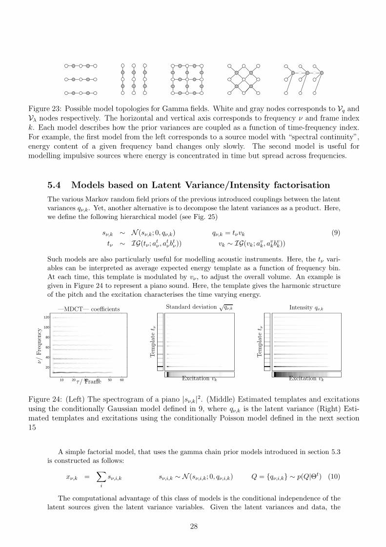
Figure 23: Possible model topologies for Gamma fields. White and gray nodes corresponds to Vq andVλ nodes respectively. The horizontal and vertical axis corresponds to frequency ν and frame indexk. Each model describes how the prior variances are coupled as a function of time-frequency index.For example, the first model from the left corresponds to a source model with “spectral continuity”,energy content of a given frequency band changes only slowly. The second model is useful formodelling impulsive sources where energy is concentrated in time but spread across frequencies.

5.4 Models based on Latent Variance/Intensity factorisation

The various Markov random field priors of the previous introduced couplings between the latentvariances qν,k. Yet, another alternative is to decompose the latent variances as a product. Here,we define the following hierarchical model (see Fig. 25)

sν,k ∼ N (sν,k; 0, qν,k) qν,k = tνvk (9)

tν ∼ IG(tν ; atν , a

tνb

tν)) vk ∼ IG(vk; av

k, avkb

vk))

Such models are also particularly useful for modelling acoustic instruments. Here, the tν vari-ables can be interpreted as average expected energy template as a function of frequency bin.At each time, this template is modulated by vν , to adjust the overall volume. An example isgiven in Figure 24 to represent a piano sound. Here, the template gives the harmonic structureof the pitch and the excitation characterises the time varying energy.

10 20 30 40 50 60

20

40

60

80

100

120

τ/ Frame

ν/

Fre

quen

cy

—MDCT— coefficients

Tem

pla

tet ν

Excitation vk

Standard deviation√qν,k

Tem

pla

tet ν

Excitation vk

Intensity qν,k

Figure 24: (Left) The spectrogram of a piano |sν,k|2. (Middle) Estimated templates and excitationsusing the conditionally Gaussian model defined in 9, where qν,k is the latent variance (Right) Esti-mated templates and excitations using the conditionally Poisson model defined in the next section15

A simple factorial model, that uses the gamma chain prior models introduced in section 5.3is constructed as follows:

xν,k =∑

i

sν,i,k sν,i,k ∼ N (sν,i,k; 0, qν,i,k) Q = {qν,i,k} ∼ p(Q|Θt) (10)

The computational advantage of this class of models is the conditional independence of thelatent sources given the latent variance variables. Given the latent variances and data, the

28

vi,0 · · · vi,k · · · vi,K−1

tν,i

sνi,0 · · · sν

i,k · · · sνi,K−1

ν = 0 . . . W − 1

y0 yk yK−1

vi,0 · · · vi,k · · · vi,K−1

tν,i

sνi,0 · · · sν

i,k · · · sνi,K−1

i = 1 . . . I

xν,0 xν,k xν,K−1

ν = 0 . . . W − 1

y0 yk yK−1

Figure 25: (Left) Latent variance/intensity models in product form (Eq.9). Hyperparameters arenot shown. (Right) Factorial version of the same model, used for polyphonic estimation as used insection 5.5.3.

posterior of the sources is a product of Gaussian distributions. In particular, the individualmarginals are given in closed form as

p(sν,i,k|X,Q) = N (sν,i,k;κν,i,kxν,k, qν,i,k(1 − κν,i,k))

κν,i,k = qν,i,k/∑

i′

qν,i′,k

This means that if the latent variances can be estimated, source separation can be easily ac-complished. The choice of prior structures on the latent variances p(Q|·) is key here.

Below we illustrate this approach in single channel source separation for transient/harmonicdecomposition. Here, we assume that there are two sources i = 1, 2. The prior variances of thefirst source i = 1 are tied across time frames using a gamma chain and aims to model a sourcewith harmonic continuity. The prior has the form

∏

ν p(qν,i=1,1:K). This model simply assumesthat for a given source the amount of energy in a frequency band stays roughly constant. Thesecond source i = 2 is tied across frequency bands and has the form

∏

k p(q1:W,i=2,k); thismodel tries to capture impulsive/percusive structure (for example compare the piano and congaexamples in Fig.4). The model aims to separate the sources based on harmonic continuity andimpulsive structure.

We illustrate this approach to separate a piano sound into its constituent components anddrum separation. We assume that J = 2 components are generated independently by twoGamma chain models with vertical and horizontal topology. In figure 26-(b), we observe thatthe model is able to separate transients and harmonic components. The sound files of theseresults can be downloaded and listened at the following url: http://www-sigproc.eng.cam.

ac.uk/~sjg/haba, which is perhaps the best way assess the sound quality.The variance/intensity factorisation models described in Eq. 9 have also straightforward

factorial extensions

xν,k =∑

i

sν,i,k

sν,i,k ∼ N (sν,i,k; 0, qν,i,k) qν,i,k = tν,ivi,k (11)

T = {tν,i} ∼ p(T |Θt) V = {vi,k} ∼ p(V |Θv) (12)

29

Time (τ)

Fre

quen

cy B

in (ν

)

Xorg

Shor

Sver

Figure 26: Single channel Source Separation example, left to right, log-MDCT coefficients of theoriginal signal and reconstruction with horizontal and vertical IGMRF models.

If we integrate out the latent sources, the marginal is given as

xν,k ∼ N (xν,k; 0,∑

i

tν,ivi,k)

Note that, as∑

i tν,ivi,k = [TV ]ν,k, the variance “field” Q is given compactly as the matrixproduct Q = TV . This resembles closely a matrix factorisation and is used extensively in audiomodelling. In the next section, we discuss models of this type.

5.5 Non-negative Matrix factorisation models

Until now, we have described conditionally Gaussian models. Recently, a popular branch ofsource separation and analysis of musical audio literature has focused on non-negativity of the

magnitude spectrogram X = {xν,τ} with xν,τ ≡ ‖sν,k‖1/22 , where sν,k are expansion coefficients

obtained from a time frequency expansion. The basic idea is representing a spectrogram byenforcing a factorisation as X ≈ TV where both T and V are matrices with positive entries(Smaragdis and Brown 2003; Abdallah and Plumbley 2006; Virtanen 2006; Kameoka 2007;Bertin, Badeau, and Richard 2007; Vincent, Bertin, and Badeau 2008). In music signal analysis,T can be interpreted as a codebook of templates, corresponding to spectral shapes of individualnotes and V is the matrix of activations, somewhat analogous to a musical score. Often, thefollowing objective is minimised:

(T, V )∗ = minT,V

D(X||TV ) (13)

where D is the information (Kullback-Leibler) divergence, given by

D(X||Λ) =∑

ν,τ

(

xν,τ logxν,τ

λν,τ− xν,τ + λν,τ

)

(14)

Using Jensen’s inequality (Cover and Thomas 1991) and concavity of log x, it can be shown ,that D(·) is nonnegative and D(X||Λ) = 0 if and only if X = Λ. The objective in (13) couldbe minimised by any suitable optimisation algorithm. (Lee and Seung 2000) have proposed anefficient variational bound minimisation algorithm that has attractive convergence properties,that has been since successfully applied to various applications in signal analysis and sourceseparation. Although not widely acknowledged, it can be shown that the minimisation algorithmis in fact an EM algorithm with data augmentation (Cemgil 2008). More precisely, it can beshown that minimising D w.r.t., T and V is equivalent finding the ML solution of the following

30

hierarchical model

xν,k =∑

i

sν,i,k

sν,i,k ∼ PO(sν,i,k; 0, λν,i,k) λν,i,k = tν,ivi,k (15)

tν,i ∼ G(tν,i; atν,i, b

tν,i/a

tν,i) vi,k ∼ G(vi,k; a

vi,k, b

vi,k/a

vi,k) (16)

The computational advantage of this models is the conditional independence of the latentsources given the variance variables. In particular, we have

p(sν,i,k|X,T, V ) = BI(sν,i,k;xν,k, κν,i,k)

κν,i,k = λν,i,k/∑

i′

λν,i′,k

This means that if the latent variances can be estimated somehow, source separation can beeasily accomplished as E(s)BI(s;x,κ) = κx.

5.5.1 Variational Bayes

It is also possible to estimate the marginal likelihood p(X) by integrating out all the templatesand excitations. This can be done via Gibbs sampling or using a variational approach. Thevariational approach is very similar to the EM algorithm, with an additional approximationstep. We sketch here the Variational Bayes (VB) (Ghahramani and Beal 2000; Bishop 2006)method to bound the marginal loglikelihood as

LX(Θ) ≡ log p(X|Θ) ≥∑

S

∫

d(T, V )q logp(X,S, T, V |Θ)

q(17)

= E(log p(X,S, V, T |Θ))q +H[q] ≡ BV B [q] (18)

where, q = q(S, T, V ) is an instrumental distribution and H[q] is its entropy. The bound istight for the exact posterior q(S, T, V ) = p(S, T, V |X,Θ), but as this distribution is complex weassume a factorised form for the instrumental distribution by ignoring some of the couplingspresent in the exact posterior

q(S, T, V ) = q(S)q(T )q(V ) =

(

∏

ν,τ

q(sν,1:I,τ )

)

∏

ν,i

q(tν,i)

∏

i,τ

q(vi,τ )

≡∏

α∈C

qα

where α ∈ C = {{S}, {T}, {V }} denotes set of disjoint clusters. Hence, we are no longerguaranteed to attain the exact marginal likelihood LX(Θ). Yet, the bound property is preservedand the strategy of VB is to optimise the bound. Although the best q distribution respecting thefactorisation is not available in closed form, it turns out that a local optimum can be attainedby the following fixed point iteration:

q(n+1)α ∝ exp

(

E(log p(X,S, T, V |Θ))q(n)¬α

)

(19)

where q¬α = q/qα. This iteration monotonically improves the individual factors of the q dis-tribution, i.e. B[q(n)] ≤ B[q(n+1)] for n = 1, 2, . . . given an initialisation q(0). The order is notimportant for convergence, one could visit blocks in arbitrary order. However, in general, theattained fixed point depends upon the order of the updates as well as the starting point q(0)(·).This approach is computationally rather attractive and is very easy to implement (Cemgil 2008).

31

5.5.2 Variational update equations and sufficient statistics

The expectations of E(log p(X,S, T, V |Θ)) are functions of the sufficient statistics of q. Thefixed point iteration for the latent sources S (where mν,τ = 1), and excitations V leads to thefollowing

q(sν,1:I,τ ) = M(sν,1:I,τ ;xν,τ , pν,1:I,τ ) q(vi,τ ) = G(

vi,τ ;αvi,τ , β

vi,τ

)

(20)

pν,i,τ = exp(E(log tν,i) + E(log vi,τ ))/∑

i

exp(E(log tν,i) + E(log vi,τ )) (21)

αvi,τ = av

i,τ +∑

ν

mν,τE(sν,i,τ ) βvi,τ =

(

avi,τ

bvi,τ+∑

ν

mν,τE(tν,i)

)−1

(22)

The variational parameters of q(tν,i) = G(

tν,i;αtν,i, β

tν,i

)

are found similarly. The hyperparam-

eters can be optimised by maximising the variational Bound. While this does not guaranteeto increase the true marginal likelihood, it leads in this application to quite practical and fastalgorithms.

5.5.3 Example: Polyphonic pitch estimation

In this section, we illustrate Bayesian NMF for polyphonic pitch detection. The approachconsists of two stages:

1. Estimation of hyperparameters given a corpus of piano notes

2. Estimation of templates and excitations given new polyphonic data and fixed hyperpa-rameters

In the first stage, we estimate the hyperparameters atν,i = at

i and btν,i (see Eq. 16), viamaximisation of the variational bound given in Eq. 18. Here, the observations are matricesXi matrix is a spectrogram computed given each note i = 1 . . . I. In figure 27, we show theestimated scale parameters btν,i as a function of frequency band ν and note index i. The harmonicstructure of each note is clearly visible.

To test the approach, we synthesize a music piece (here, a short segment from the beginningof “Fur Elise” by Beethoven), given a midi piano roll and recordings of isolated notes from apiano by simply appropriately shifting each time series and adding. The piano roll and thethe spectrogram of the synthesized audio are shown in Figure 28. The pitch detection task isinfering the excitations given the hyperparameters and the spectrogram.

The results are shown in Figure 29. The top figure shows the excitations estimated give theprior Eq. 16. The notes are visible here but there are some artifacts. The middle figure showsresults from a model where excitations are tied across time using a Gamma chain introducedin section 5.3. This prior is highly effective here and we are able to get a more clearer picture.The bottom figure displays results obtained from a real recording of “Fur Elise”, performed onelectric guitar. Interestingly, whilst we are still using the hyperparameters estimated from apiano, the infered excitations show significant overlap with the original score.

6 Probabilistic Models for Tempo, Rhythm, Meter

An important feature of music information retrieval and interactive performance systems is thecapacity to infer attributes related to the temporal structure of audio signals. Detecting thepulse or foot-tapping rate of musical audio signals has been a focus of research in musical signalprocessing for several years (Cemgil 2004; Klapuri and Davy 2006). However, little attentionhas been paid to the task of extracting information about the more abstract musical concepts

32

i/Key index

ν/F

requ

ency

inde

x

Estimated Scale Parameters of the template prior

10 20 30 40 50 60 70 80

50

100

150

200

250

300

350

400

450

500

Figure 27: Estimated template hyperparameters btν,i.

Not

e In

dex

Frame

Piano Roll

τ/Frame

ν/F

requ

ency

Bin

Log |MDCT| coefficients

50 100 150 200 250

50

100

150

200

250

300

350

400

450

500

Figure 28: The ground truth piano roll and the spectrum of the polyphonic data

33

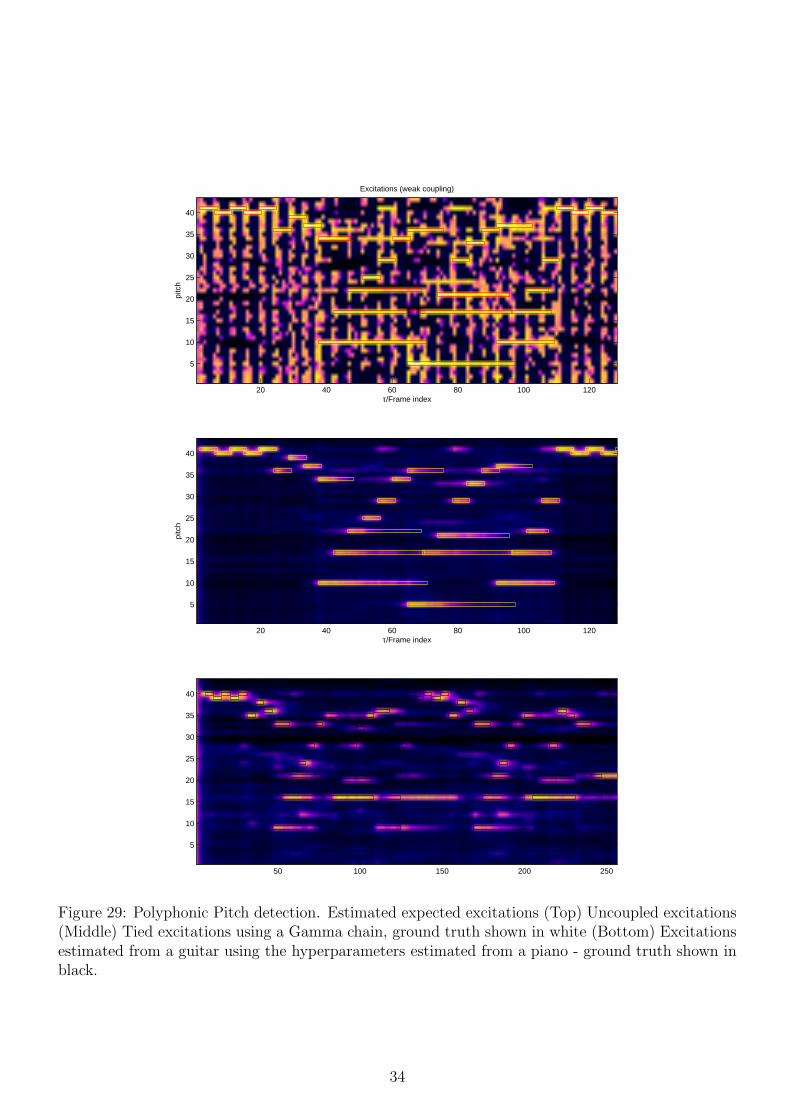
τ/Frame index

pitc

h

Excitations (weak coupling)

20 40 60 80 100 120

5

10

15

20

25

30

35

40

pitc

h

τ/Frame index20 40 60 80 100 120

5

10

15

20

25

30

35

40

50 100 150 200 250

5

10

15

20

25

30

35

40

Figure 29: Polyphonic Pitch detection. Estimated expected excitations (Top) Uncoupled excitations(Middle) Tied excitations using a Gamma chain, ground truth shown in white (Bottom) Excitationsestimated from a guitar using the hyperparameters estimated from a piano - ground truth shown inblack.

34

of tempo, rhythm and meter. An hierarchical Bayesian approach is ideally suited to this task.In order to quantify the musical concepts of interest, we interpret tempo as being equivalentto the performed rate of quarter notes and rhythmic pattern as indicating the regions within amusical bar in which note onsets are likely to occur. In this section we summarise a modellingframework which permits inference of these quantities from observed MIDI onset events or rawaudio samples (Whiteley, Cemgil, and Godsill 2006; Whiteley, Cemgil, and Godsill 2007).

6.1 A Bar-pointer Model

Central to the method is a dynamical model of a bar-pointer, an hypothetical, hidden, dynamicalobject which maps the positive real line to one period of a latent rhythmical pattern, i.e. onemusical bar. Different rhythms are represented by rhythmic pattern functions which controlthe hyper-parameters of a conjugate gamma-Poisson observation model. The trajectory of thebar-pointer modulates these functions onto the time line. Conditional upon this trajectory andhyper-parameter values, observed MIDI onset events are modelled as being a non-homogeneousPoisson Process or raw audio samples are modelled as being a Gaussian process. The inferencetask is then to estimate the state of the bar-pointer and values of rhythmic pattern indicatorvariables. Both filtering and smoothing are of interest in different applications.

For a discrete time index k and ∆ a positive constant, at time tk = k∆ denote by φk

the position of the bar-pointer, which takes values in [0, 1). Denote by φk its velocity whichtakes values in [φmin, φmax], where φmin > 0 and φmax represents the mximum tempo to beconsidered. The motion of the bar-pointer is modelled as being a piece-wise constant velocityprocess:

φk+1 = (φk + ∆φk)mod 1,

p(φk+1|φk) ∝ N (φk, σ2φ) × I[φmin≤φk+1≤φmax],

where I[x] takes the value 1 when x is true and zero otherwise. The velocity of the bar pointeris defined to be proportional to tempo.

At each time index k, a rhythmic pattern indicator, Rk, takes one value in a finite set, forexample S = {0, 1}. The elements of the set S correspond to different rhythmic patterns, whichare described in further detail below, with examples given in figure 30. For now we deal withthe simple case in which there are only two such patterns, and switching between values of Rk

is modelled as occurring if a bar line is crossed, i.e.:

if φk < φk−1,

Pr(Rk = s|rk−1, φk, φk−1) =

{

pr, s 6= rk−1,1 − pr, s = rk−1,

otherwise, Rk = rk−1, where pr is the probability of a change in rhythmic pattern. In summary,xk ≡ [φk φk rk]

T specifies the state of the system at time index k. We remark that the dynamicalmodel can be extended to include the musical notion of meter, see (Whiteley, Cemgil, and Godsill2006) for details.

6.2 Poisson Observation Model

MIDI onset events are treated as being Poisson distributed with an intensity parameter which isconditioned on the position of the bar-pointer and the rhythm indicator variable. Defining thePoisson intensity in this fashion allows quantification of the postulate that for a given rhythm,there are regions in one bar in which onsets occur with high probability.

Each rhythmic pattern function, µr : [0, 1) → R+, maps the position of the bar pointer φk

to the mean of a gamma prior distribution on an intensity parameter λk. The value of µr(φk)

35

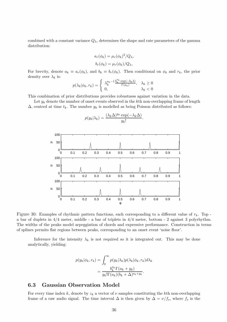
combined with a constant variance Qλ, determines the shape and rate parameters of the gammadistribution:

ar(φk) = µr(φk)2/Qλ,

br(φk) = µr(φk)/Qλ,

For brevity, denote ak ≡ ar(φk), and bk ≡ br(φk). Then conditional on φk and rk, the priordensity over λk is:

p(λk|φk, rk) =

{

λak−1k

bakk

exp(−bkλ)

Γ(ak) , λk ≥ 0

0, λk < 0

This combination of prior distributions provides robustness against variation in the data.Let yk denote the number of onset events observed in the kth non-overlapping frame of length

∆, centred at time tk. The number yk is modelled as being Poisson distributed as follows:

p(yk|λk) =(λk∆)yk exp(−λk∆)

yk!.

0 0.1 0.2 0.3 0.4 0.5 0.6 0.7 0.8 0.9 10

50

100

µ

0 0.1 0.2 0.3 0.4 0.5 0.6 0.7 0.8 0.9 10

50

100

µ

0 0.1 0.2 0.3 0.4 0.5 0.6 0.7 0.8 0.9 10

50

100

µ

φ

Figure 30: Examples of rhythmic pattern functions, each corresponding to a different value of rk. Top -a bar of duplets in 4/4 meter, middle - a bar of triplets in 4/4 meter, bottom - 2 against 3 polyrhythm.The widths of the peaks model arpeggiation of chords and expressive performance. Construction in termsof splines permits flat regions between peaks, corresponding to an onset event ‘noise floor’.

Inference for the intensity λk is not required so it is integrated out. This may be doneanalytically, yielding:

p(yk|φk, rk) =

∫ ∞

0p(yk|λk)p(λk|φk, rk)dλk

=bak

k Γ(ak + yk)

yk!Γ(ak)(bk + ∆)ak+yk.

6.3 Gaussian Observation Model

For every time index k, denote by zk a vector of ν samples constituting the kth non-overlappingframe of a raw audio signal. The time interval ∆ is then given by ∆ = ν/fs, where fs is the

36

sampling rate. The samples are modelled as independent with a zero mean Gaussian distribu-tion:

p(zk|σ2k) =

1

(2πσ2k)ν/2

exp

(

−zTk zk2σ2

k

)

.

An inverse-gamma distribution is placed on the variance σ2k. The shape and scale parameters

of this distribution, denoted by ck and dk respectively, are determined by the location of thebar pointer, φk and the rhythmic pattern indicator variable rk, again via a rhythmic patternfunction, µk.

p(σ2k|φk, rk) =

dck

k exp(−dk/σ2z)

Γ(ck)σ−2(ck+1)k ,

ck = µ2k/Qs + 2,

dk = µk

(

µ2k

Qs+ 1

)

,

where Qs is the variance of the inverse-gamma distribution and is chosen to be constant.The variance of the Gaussian distribution, σ2

k, may be integrated out analytically to yield:

p(zk|φk, rk) =dck

k Γ(ck + ν/2)

(2π)ν/2Γ(ck)

(

zTk zk2

+ dk

)−(ck+ν/2)

.

6.4 Results

Of practical interest are the posterior filtering and smoothing distributions, e.g for some daterecord of length K frames, p(φ1:K , φ1:K , r1:K |y1:K) and its marginals.

The performance of this model is demonstrated by a smoothing task for an excerpt of aMIDI performance of ‘Michelle’ by the Beatles, using the Poisson observation model (results forthe Gaussian observation model are reported in (Whiteley, Cemgil, and Godsill 2006)). Thisdemonstrates the joint tempo-tracking and rhythm recognition capability of the method. Theperformance, by a professional pianist, was recorded using a Yamaha Disklavier C3 Pro GrandPiano. The top two rhythmic patterns in figure 30 were employed. For purposes of exposition,the state-space of the bar pointer was uniformally discretised to M = 1000 position and N = 20velocity points. The discretised position and velocity of bar pointer are denoted by mk and nk

respectively, with the discretised dynamical model being that with probability 0.99, nk = nk−1

and, within the allowed range, nk is incremented or decremented with equi-probability. Uniforminitial prior distributions were set onmk, nk and rk. The time frame length was set to ∆ = 0.02s,corresponding to the range of tempi: 12 − 240 quarter notes per minute. The probability of achange in rhythmic pattern was set to pr = 0.1. The variance of the gamma distribution wasset Qλ = 10.

This section of ‘Michelle’ presents a significant challenge for tempo tracking because of thetriplets, each of which by definition has a duration of 3/2 quarter notes. A performance of thisexcerpt could be wrongly interpreted as having a local change in tempo in the second bar, whenin fact the rate of quarter notes remains constant; the bar of triplets is just a change in rhythm.

For the discretised model, exact inference is possible (Sequential Monte Carlo methods forthe non-discretised model are investigated in (Whiteley, Cemgil, and Godsill 2007)). In figure31, the strong diagonal stripes in the image of the posterior smoothing distributions for mk

correspond to the maximum a-posteriori (MAP) trajectory of the bar pointer. The change toa triplet rhythm in the second bar and the subsequent reversion to duplet rhythm are correctlyidentified. The MAP tempo is given by the darkest stripe in the image for the velocity log-smoothing distribution - it is roughly constant throughout.

37

0 50 100 150 200 250 300 350 400 4500

1

2

y k

Observed Data

mk

log p(mk|y

1:K)

50 100 150 200 250 300 350 400 450

800

600

400

200 −10

−5

0

Qua

rter

not

es p

er m

in. log p(n

k|y

1:K)

50 100 150 200 250 300 350 400 450

180

120

60−10

−5

0

p(rk|y

1:K)

Frame Index, k

50 100 150 200 250 300 350 400 450

Triplets

Duplets 0.20.40.60.8

Figure 31: Results for joint tempo tracking and rhythmic pattern recognition on a MIDI performanceof ‘Michelle’ by the Beatles. The top figure is the score which the pianist was given to play. Eachimage consists of smoothing marginal distributions for each frame index.

7 Discussion and Conclusions

In this review, we sketched Bayesian methods for analysis of audio signals. The Bayesian modelsexhibit complex statistical structure and in practice, highly adaptive and powerful computa-tional techniques are needed to perform inference.

In this chapter, we have reviewed some of these statistical models, including generalised linearmodels, dynamic systems and other hierarchical models, and described how various problemsin audio and music processing can be cast into Bayesian posterior inference. We have alsoillustrated inference methods based on Monte Carlo simulation or other deterministic techniques(such as mean field, variational Bayes) originating in statistical physics to tackle computationalproblems posed by inference in these models. We describes models in both the time domain andtransform domains, the latter typically offering greater computational tractability and modellingflexibility at the expense of some accuracy in the models.

The Bayesian approach has two key advantages over more traditional engineering solutions:it provides both a suite for model construction and a framework for algorithm development.Apart from the pedagogical advantages (such as highlighting algorithmic similarities, conver-gence characteristics and computational requirements), the framework facilitates developmentof sophisticated models and to automation of code generation procedures. We believe that thefield of computer hearing, which is still in its infancy compared to topics such as computervision and speech recognition, has great potential for advancement in coming years, with theadvent of powerful Bayesian inference methodologies and accompanying computational powerincreases.

38

A Review of sinusoidal models

This appendix introduces several low-level, deterministic representations of audio signals andhighlights the links between various representations such as damped sinusoids, state space andGabor representations. In the main text, these representations are used to formulate statisticalmodels for observed data, given the values of latent parameters. These deterministic representa-tions are highly structured and the statistical models into which they are assimilated thereforeexhibit rich temporal and spectral properties. Furthermore, the specific parameterisations ofthese signal models allows their statistical counter-parts to be coupled to higher-level modelcomponents, such as change-point processes and model-order indicators.

A.1 Static Models

Sound signals are emitted by vibrating objects that can be modelled as a cascade of secondorder systems. Hence, it is convenient to represent them as a sum of sinusoids and a transientnon-periodic component (See e.g. (McAulay and Quatieri 1986; Serra and Smith 1991; Rodet1998; Irizarry 2002; Parra and Jain 2001; Davy and Godsill 2003)). We will start our expositionusing a deterministic and static model, which we later generalise in several directions. For atime series yn of length N with n = 0 . . . N − 1, the (deterministic) discrete time sinusoidalmodel can be written as

yn =W−1∑

ν=0

ανe−γνn cos(ωνn+ φν) (23)

Here, ν = 0 . . .W − 1 denotes the sinusoidal index and W is the total number of sinusoidalcomponents. The parameters of this model are all real numbers, amplitudes αν , log-dampingcoefficients γν > 0, the frequencies ων and the phases φν . Using the fact that cos(θ) = (ejθ +e−jθ)/2 we can write

yn =W−1∑

ν=0

(cνznν + c∗νz

∗νn) (24)

where cν is the complex amplitude cν = (αν/2)ejφν and zν is the complex pole zν = e−γν+jων .

It is obvious that we can write the model in matrix notation as:

y ≡

y0

y1...yn...

yN−1

=

1 1 . . . 1 1z0 z∗0 . . . zW−1 z∗W−1...

......

......

zn0 z∗0

n . . . znW−1 z∗nW−1

......

......

...

zN−10 z∗0

N−1 . . . zN−1W−1 z∗N−1

W−1

c0c∗0...

cW−1

c∗W−1

≡ F0:N−1c

F0:N−1 = F0:N−1(γ,ω) is N × 2W and each column is a damped complex exponential. Then + 1’th row will be denoted as Fn. It is possible to estimate all parameters using subspacetechniques (Laroche 1993; Badeau, Boyer, and David 2002).

Many popular models appear as special cases of the above model, and can be obtainedby tying various parameters. The harmonic model, with fundamental frequency ω and somelog-damping coefficient γ is defined as (23) by the following

ων = νω γν = νγ (25)

39

This model is particularly useful for pitched musical instruments that tend to create oscillationswith modes that are roughly related by integer ratios. It is possible to let the damping coeffi-cients free; or tie them as above to model the fact that higher frequencies get damped faster. Arelated model is the inharmonic model that assumes

ων = B(ν, ω) (26)

where B is a function that “stretchs” the harmonic frequencies. Stretching of harmonics is aphenomena that is observed especially in piano strings.

It is important to note that the inverse Fourier transform is obtained as a special case of theharmonic model by ignoring the damping γν = γ = 0 and choosing the frequencies on a uniformgrid with ων = 2πν/N for ν = 0 . . . W − 1 with W = N/2. We call all these models and theirvariations static models.

A.2 State space Representations and Dynamic Models

An alternative, dynamic representation exploits the rotational invariance property:

yn

yn+1...

yn+L−1

=

1 1 . . . 1 1z0 z∗0 . . . zW−1 z∗W−1...

......

......

zL−10 z∗0

L−1 . . . zL−1W−1 z∗L−1

W−1

z0z∗0

. . .

zW−1

z∗W−1

n

c0c∗0...

cW−1

c∗W−1

yn:n+L−1 = F0:L−1 diag(Z0, Z1, . . . , ZW−1)nc (27)

with Zν = Zν(γν , ων) ≡ diag(zν , z∗ν), c ≡

(

c0 c∗0 . . . cW−1 c∗W−1

)⊤. By appropriately

rotating the complex amplitudes, the basis matrix stays shift invariant in time. This representa-tion allows us to write a model for arbitrary frame lengths and “interpolate” between dynamicand static interpretations. For example, given a suitable frame length L, we can reorganise thetime series in N/L nonoverlapping frames (assuming L divides N). Then we can write using(27)

yk ≡ (ykL, . . . , y(k+1)L−1)⊤ = F0:L−1 diag(ZL

0 , ZL1 , . . . , Z

LW−1)

kc

Here, k denotes a frame index such that k = 0 . . . N/L − 1. One can easily envision modelswhere subsequent frames are possibly of different length Lk such that

∑

k Lk = N . Of course,mathematically speaking, we haven’t really gained anything and in the noiseless case, all for-mulations for any frame length L are equivalent. However, the dynamical system perspectiveopens up interesting possibilities to extend the basic model in a way that is not apparent in thestatic formulation. In particular, we can write the following state space parametrisation:

sd0 =(

c0 c∗0 . . . cW−1 c∗W−1

)⊤= c

sdk+1 = Adsdk

yk = F0:L−1sdk

where Ad ≡ diag(ZL1 , Z

L2 , . . . , Z

LW−1) is a 2W × 2W diagonal matrix with poles appearing in

conjugate pairs and F0:L−1 is L × 2W , as defined in (27). This representation is known asthe diagonal realisation. It is well known that the representation of yk is not unique; for anyinvertible transform matrix T , we could define sk = T sdk

T sdk+1 = T AdT −1T sdk ⇐⇒ sk+1 = Ask (28)

yk = F0:L−1T −1T sdk ⇐⇒ yk = C0:L−1sk (29)

40

with new state evolution and observation matrices A ≡ T AdT −1 and C0:L−1 ≡ F0:L−1T −1. Inparticular, to avoid complex arithmetic, one can apply the following block diagonal transform

T = diag(T, T, . . . , T ) (30)

T ≡ 1√2

(

1 1j −j

)

TTH = THT = I

This renders the n+ 1’th row of C0:L−1

Cn = FnT H (31)

=√

2(

e−nγ0 cos(nω0) e−nγ0 sin(nω0) . . . e−nγW−1 cos(nωW−1) e−nγW−1 sin(nωW−1))

(32)

Further we obtain

A = diag(A0, . . . , Aν , . . . , AW−1) (33)

Aν = Aν(γν , ων) = TZLν T

H = e−Lγν

(

cos(Lων) − sin(Lων)sin(Lων) cos(Lων)

)⊤

s0 =(

s⊤0,0 . . . s⊤0,ν . . . s⊤0,W−1

)⊤(34)

s0,ν = T(

cν c∗ν)⊤

=√

2(

Re {cν} −Im {cν})⊤

The harmonic and inharmonic models of the previous section can be written in state spaceform by constraining the poles to have related frequencies. For example, the harmonic modelwith damping coefficient γ and fundamental frequency ω can be written as

Aν = Aν(γν , ων) = TZ(γ, ω)LνTH = e−Lγν

(

cos(Lων) − sin(Lων)sin(Lων) cos(Lων)

)⊤

A.3 Nonstationarity and Time-Frequency Representations

The sinusoidal model, as we have introduced it in the previous section, is rather restrictivefor modelling long sequences and realisations from nonstationary processes, as the poles of themodel are taken to be fixed. One possibility is to assume that the poles are time varying; whereone can take

Aν,k = Aν(γν,k, ων,k) Ck = C(γ0:W−1,k, ω0:W−1,k)

However, the associated estimation problem is highly nonlinear. The inverse problem is alsoill posed as one can generate any signal if one can arbitrarily modulate the pole frequenciesand damping coefficients. Hence, an appropriate regulariser, such as a random walk in polefrequencies, needs to be assumed. In certain cases, such as when the harmonic model is used, thepole frequencies can be discretised and deterministic grid based inference techniques (Tabrikian,Dubnov, and Dikalov 2004; Cemgil, Kappen, and Barber 2004) or more powerful sequentialMonte Carlo techniques can be employed (Dubois and Davy 2007).

An arguably simpler approach is to use a basis that is localised both in time and frequency.Such representations are known as Gabor representations. In the Gabor representation (Mallat1999; Wolfe, Godsill, and Ng 2004), a real valued time series is represented on a W ×K time-frequency lattice by

yn =

K−1∑

τ=0

W−1∑

ν=0

(

cν,τhn,τznν + c∗ν,τhn,τz

∗νn)

41

where ν = 0 . . . W − 1 is the frequency band index and τ = 0 . . . K − 1 is the time frame index,where the poles are zν = zν(ω) = ejων with ω = 2π/W . The coefficients hn,τ are fixed and aredetermined from a prototype window function h(n) as

hn,τ = h(n− τN

K)

The real valued and non-negative window function is typically chosen as a symmetric bell-shapedcurve with compact support5 to give a suitable time-frequency localisation. The ratio N/Kdenotes the effective number of samples that we shift the window with each frame. The ratioKW/N is the oversampling rate and gives an indication of the redundancy of the representation.It is informative to write the model in matrix form

y = Gc

where the expansion coefficients are given as

c =(

c0,0 c∗0,0 . . . c1,τ . . . cν,1 . . . c∗W−1,K−1

)⊤

and G is given as a N × 2WK matrix

g0,0(0) g∗0,0(0) . . . g0,τ (0) . . . gν,0(0) . . . g∗W−1,K−1(0)... . . . . . .

......

......

g0,0(n) g∗0,0(n) . . . g0,τ (n) . . . gν,0(n) . . . g∗W−1,K−1(n)... . . . . . .

......

... . . ....

g0,0(N − 1) g∗0,0(N − 1) . . . g0,τ (N − 1) . . . gν,0(N − 1) . . . g∗W−1,K−1(N − 1)

(35)

Here, each column is a basis vector with a modulated and translated version of the windowfunction gν,τ (n) = hn,τz

nν . To avoid complex arithmetic, the block diagonal transformation in

(30) can be employed as y = GT −1T c = Gs to obtain real matrices and expansion coefficients,as in (32) and (34). For certain choices of the time-frequency lattice parameters with KW = N ,the matrix G can be rendered square and orthonormal GHG = I. One such choice is taking thewindow h rectangular with a support of L = N/K samples such that subsequent windows do notoverlap in time and using W = L frequency bins. This is equivalent to modelling the sequenceas independent time frames. Many other techniques, such as lapped orthogonal transforms ormodified discrete cosine transforms, to obtain orthagonality with other type of window andbasis functions exist and it is beyond our purpose to review this rather broad literature.

The Gabor representation is in a way a generalisation of the sinusoidal model in Eq. (24),that represents the signal by exponentially decaying window function e−γn, using a single sinu-soid per frequency band. In contrast, the Gabor representation chooses at each time frame andeach frequency band a new expansion coefficient, hence does not enforce phase continuity andallows for smooth amplitude variations. One potential shortcomming of the Gabor representa-tion is that it is not very powerful in representing abrupt changes in the signal characteristics,such as chaingepoints or frequency modulations.

References

Abdallah, S. A. and M. D. Plumbley (2006, January). Unsupervised analysis of polyphonicmusic using sparse coding. IEEE Transactions on Neural Networks 17 (1), 179–196.

5However, the original paper by Gabor assumed Gaussian functions with infinite support

42

Badeau, R., R. Boyer, and B. David (2002, September). Eds parametric modelling and track-ing of audio signals. In DAFx-02, Hamburg, Germany.

Bertin, N., R. Badeau, and G. Richard (2007). Blind signal decompositions for automatictranscription of polyphonic music: NMF and K-SVD on the benchmark. In Proc. ofInternation conference on audio, speech and signal processing (ICASSP), Honolulu.

Bishop, C. M. (2006). Pattern Recognition and Machine Learning. Springer.

Cemgil, A. T. (2004). Bayesian Music Transcription. Ph. D. thesis, Radboud University ofNijmegen.

Cemgil, A. T. (2007). Strategies for sequential inference in factorial switching state spacemodels. In Proc. of IEEE Int. Conf. on Acoustics, Speech and Signal Processing (ICASSP07), Honolulu, Hawaii, pp. 513–516.

Cemgil, A. T. (2008, July). Bayesian inference in non-negative matrix factorisation models.Technical Report CUED/F-INFENG/TR.609, University of Cambridge.

Cemgil, A. T. and O. Dikmen (2007, September). Conjugate gamma Markov random fieldsfor modelling nonstationary sources. In ICA 2007, 7th International Conference on Inde-pendent Component Analysis and Signal Separation.

Cemgil, A. T., S. J. Godsill, and C. Fevotte (2007). Variational and Stochastic Inference forBayesian Source Separation. Digital Signal Processing 17.

Cemgil, A. T., H. J. Kappen, and D. Barber (2004). A generative model for music transcrip-tion. Accepted to IEEE Transactions on Speech and Audio Processing .

Cemgil, A. T., P. Peeling, O. Dikmen, and S. J. Godsill (2007, October). Prior structures fortime-frequency energy distributions. In Accepted to Proc. of IEEE Workshop on Applica-tions of Signal Processing to Audio and Acoustics.

Cover, T. M. and J. A. Thomas (1991). Elements of Information Theory. New York: JohnWiley & Sons, Inc.

Davy, M., S. Godsill, and J. Idier (2006, April). Bayesian analysis of polyphonic western tonalmusic. Journal of the Acoustical Society of America 119 (4).

Davy, M. and S. J. Godsill (2002). Detection of abrupt spectral changes using support vec-tor machines. an application to audio signal segmentation. In Proc. IEEE InternationalConference on Acoustics, Speech and Signal Processing.

Davy, M. and S. J. Godsill (2003). Bayesian harmonic models for musical signal analysis. InBayesian Statistics 7.

Dubois, C. and M. Davy (2007, May). Joint detection and tracking of time-varying har-monic components: a flexible bayesian approach. IEEE transactions on Speech, Audioand Language Processing 15 (4), 1283–1295.

Fearnhead, P. (2003). Exact and efficient bayesian inference for multiple changepoint prob-lems. Technical report, Dept. of Math. and Stat., Lancaster University.

Fevotte, C., L. Daudet, S. J. Godsill, and B. Torresani (2006, May). Sparse regression withstructured priors: Application to audio denoising. In Proc. ICASSP, Toulouse, France.

Fevotte, C. and S. Godsill (2006). A Bayesian approach for blind separation of sparse sources.IEEE Trans. on Speech and Audio Processing .

Fletcher, N. H. and T. Rossing (1998). The Physics of Musical Instruments. Springer.

Ghahramani, Z. and M. Beal (2000). Propagation algorithms for variational Bayesian learn-ing. In Neural Information Processing Systems 13.

Godsill, S. (2004). Computational modeling of musical signals. Chance Magazine (AmericanStatistical Association 17 (4).

43

Godsill, S. and M. Davy (2005, October). Bayesian computational models for inharmonicityin musical instruments. In Proc. of IEEE Workshop on Applications of Signal Processingto Audio and Acoustics, New Paltz, NY.

Godsill, S. J. and M. Davy (2002). Bayesian harmonic models for musical pitch estimationand analysis. In Proc. IEEE International Conference on Acoustics, Speech and SignalProcessing.

Green, P. J. (1995). Reversible jump Markov-chain Monte Carlo computation and Bayesianmodel determination. Biometrika 82 (4), 711–732.

Grimmett, G. and D. Stirzaker (2001). Probability and Random Processes (Third Editioned.). Oxford University Press.

Hamacher, V., J. Chalupper, J. Eggers, E. Fischer, U. Kornagel, H. Puder, and U. Rass(2005). Signal processing in high-end hearing aids: state of the art, challenges, and futuretrends. EURASIP J. Appl. Signal Process. 2005 (1), 2915–2929.

Irizarry, R. A. (2002). Weighted estimation of harmonic components in a musical sound signal.Journal of Time Series Analysis 23.

Kameoka, H. (2007). Statistical Approach to Multipitch Analysis. Ph. D. thesis, University ofTokyo.

Klapuri, A. and M. Davy (Eds.) (2006). Signal Processing Methods for Music Transcription.New York: Springer.

Knuth, K. H. (1998, Jul.). Bayesian source separation and localization. In SPIE’98: BayesianInference for Inverse Problems, San diego, pp. 147–158.

Laroche, J. (1993). Use of the matrix pencil method for the spectrum analysis of musicalsignals. Journal of Acoustical Society of America 94, 1958–1965.

Lee, D. D. and H. S. Seung (2000). Algorithms for non-negative matrix factorization. InNIPS, pp. 556–562.

Mallat, S. (1999). A Wavelet Tour of Signal Processing. Academic Press.

McAulay, R. J. and T. F. Quatieri (1986). Speech analysis/synthesis based on a sinusoidalrepresentation. IEEE Transactions on Acoustics, Speech, and Signal Processing 34 (4),744–754.

McIntyre, M. E., R. T. Schumacher, and J. Woodhouse (1983). On the oscillations of musicalinstruments. J. Acoustical Society of America 74, 1325–1345.

Miskin, J. and D. Mackay (2001). Ensemble learning for blind source separation. In S. J.Roberts and R. M. Everson (Eds.), Independent Component Analysis, pp. 209–233. Cam-bridge University Press.

Mohammad-Djafari, A. (1997, Jul.). A Bayesian estimation method for detection, localisationand estimation of superposed sources in remote sensing. In SPIE’97, San Diego.

Parra, L. and U. Jain (2001). Approximate Kalman filtering for the harmonic plus noisemodel. In Proc. of IEEE WASPAA, New Paltz.

Peeling, P. H., C. Li, and S. J. Godsill (2007, April). Poisson point process modeling forpolyphonic music transcription. Journal of the Acoustical Society of America ExpressLetters 121 (4), EL168–EL175. Reused with permission from Paul Peeling, The Journalof the Acoustical Society of America, 121, EL168 (2007). Copyright 2007, AcousticalSociety of America.

Reyes-Gomez, M., N. Jojic, and D. Ellis (2005). Deformable spectrograms. In AI and StatisticsConference, Barbados.

Rodet, X. (1998). Musical sound signals analysis/synthesis: Sinusoidal + residual and ele-mentary waveform models. Applied Signal Processing .

44

Rowe, D. B. (2003). Multivariate Bayesian Statistics: Models for Source Separation andSignal Unmixing. Chapan & Hall/CRC.

Serra, X. and J. O. Smith (1991). Spectral modeling synthesis: A sound analysis/synthesissystem based on deterministic plus stochastic decomposition. Computer Music Jour-nal 14 (4), 12–24.

Shepard, N. (Ed.) (2005). Stochastic Volatility, Selected Readings. Oxford University Press.

Smaragdis, P. and J. Brown (2003). Non-negative matrix factorization for polyphonic mu-sic transcription. In WASPAA, IEEE Workshop on Applications of Signal Processing toAudio and Acoustics.

Tabrikian, J., S. Dubnov, and Y. Dikalov (2004, Jan). Maximum a-posteriori probability pitchtracking in noisy environments using harmonic model. IEEE Transactions on Speech andAudio Processing 12 (1), 76–87.

Vincent, E., N. Bertin, and R. Badeau (2008). Harmonic and inharmonic nonnegative matrixfactorization for polyphonic pitch transcription. In Proc. IEEE Int. Conf. on Acoustics,Speech and Signal Processing (ICASSP), Las Vegas. IEEE.

Virtanen, T. (2006, November). Sound Source Separation in Monaural Music Signals. Ph. D.thesis, Tampere University of Technology.

Walmsley, P., S. J. Godsill, and P. J. W. Rayner (1998, September). Multidimensional opti-misation of harmonic signals. In Proc. European Conference on Signal Processing.

Walmsley, P. J., S. J. Godsill, and P. J. W. Rayner (1999, October). Polyphonic pitch trackingusing joint Bayesian estimation of multiple frame parameters. In Proc. IEEE Workshopon Audio and Acoustics, Mohonk, NY State, Mohonk, NY State.

Wang, D. and G. J. Brown (Eds.) (2006). Computational Auditory Scene Analysis: Principles,Algorithms, Applications. Wiley.

Whiteley, N., A. T. Cemgil, and S. J. Godsill (2006). Bayesian modelling of temporal struc-ture in musical audio. In Proceedings of International Conference on Music InformationRetrieval, Victoria, Canada.

Whiteley, N., A. T. Cemgil, and S. J. Godsill (2007, April). Sequential Inference of RhythmicStructure in Musical Audio. In Proc. of IEEE Int. Conf. on Acoustics, Speech and SignalProcessing (ICASSP 07), pp. 1321–1324. IEEE.

Wolfe, P. J., S. J. Godsill, and W. Ng (2004). Bayesian variable selection and regularisationfor time-frequency surface estimation. Journal of the Royal Statistical Society .

45