bayesian statistics - ceremadexian/coursbc.pdf · bayesian statistics outline introduction...
TRANSCRIPT
Bayesian Statistics
Bayesian Statistics
Christian P. Robert
Universite Paris Dauphine and CREST-INSEEhttp://www.ceremade.dauphine.fr/∼xian
January 9, 2006
Bayesian Statistics
Outline
Introduction
Decision-Theoretic Foundations of Statistical Inference
From Prior Information to Prior Distributions
Bayesian Point Estimation
Bayesian Calculations
Tests and model choice
Admissibility and Complete Classes
Hierarchical and Empirical Bayes Extensions, and the Stein Effect
Bayesian Statistics
Introduction
Vocabulary, concepts and first examples
IntroductionModelsThe Bayesian frameworkPrior and posterior distributionsImproper prior distributions
Decision-Theoretic Foundations of Statistical Inference
From Prior Information to Prior Distributions
Bayesian Point Estimation
Bayesian Calculations

Bayesian Statistics
Introduction
Models
Parametric model
Observations x1, . . . , xn generated from a probability distributionfi(xi|θi, x1, . . . , xi−1) = fi(xi|θi, x1:i−1)
x = (x1, . . . , xn) ∼ f(x|θ), θ = (θ1, . . . , θn)
Bayesian Statistics
Introduction
Models
Parametric model
Observations x1, . . . , xn generated from a probability distributionfi(xi|θi, x1, . . . , xi−1) = fi(xi|θi, x1:i−1)
x = (x1, . . . , xn) ∼ f(x|θ), θ = (θ1, . . . , θn)
Associated likelihoodℓ(θ|x) = f(x|θ)
[inverted density]
Bayesian Statistics
Introduction
The Bayesian framework
Bayes Theorem
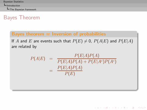
Bayes theorem = Inversion of probabilities
If A and E are events such that P (E) 6= 0, P (A|E) and P (E|A)are related by
P (A|E) =P (E|A)P (A)
P (E|A)P (A) + P (E|Ac)P (Ac)
=P (E|A)P (A)
P (E)
Bayesian Statistics
Introduction
The Bayesian framework
Bayes Theorem
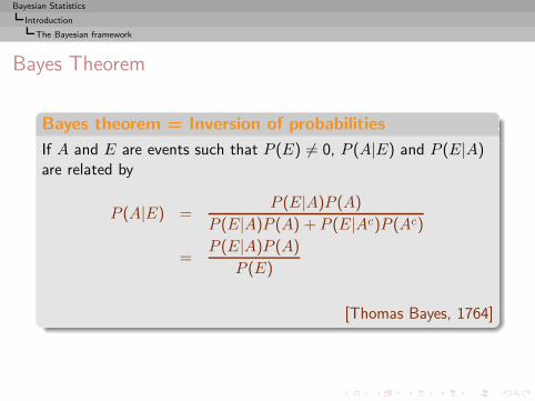
Bayes theorem = Inversion of probabilities
If A and E are events such that P (E) 6= 0, P (A|E) and P (E|A)are related by
P (A|E) =P (E|A)P (A)
P (E|A)P (A) + P (E|Ac)P (Ac)
=P (E|A)P (A)
P (E)
[Thomas Bayes, 1764]
Bayesian Statistics
Introduction
The Bayesian framework
Bayes Theorem
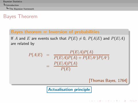
Bayes theorem = Inversion of probabilities
If A and E are events such that P (E) 6= 0, P (A|E) and P (E|A)are related by
P (A|E) =P (E|A)P (A)
P (E|A)P (A) + P (E|Ac)P (Ac)
=P (E|A)P (A)
P (E)
[Thomas Bayes, 1764]
Actualisation principle
Bayesian Statistics
Introduction
The Bayesian framework
New perspective
◮ Uncertainty on the parameter s θ of a model modeled througha probability distribution π on Θ, called prior distribution
Bayesian Statistics
Introduction
The Bayesian framework
New perspective
◮ Uncertainty on the parameter s θ of a model modeled througha probability distribution π on Θ, called prior distribution
◮ Inference based on the distribution of θ conditional on x,π(θ|x), called posterior distribution
π(θ|x) =f(x|θ)π(θ)∫f(x|θ)π(θ) dθ
.
Bayesian Statistics
Introduction
The Bayesian framework
Definition (Bayesian model)
A Bayesian statistical model is made of a parametric statisticalmodel,
(X , f(x|θ)) ,
Bayesian Statistics
Introduction
The Bayesian framework
Definition (Bayesian model)
A Bayesian statistical model is made of a parametric statisticalmodel,
(X , f(x|θ)) ,and a prior distribution on the parameters,
(Θ, π(θ)) .

Bayesian Statistics
Introduction
The Bayesian framework
Justifications
◮ Semantic drift from unknown to random
Bayesian Statistics
Introduction
The Bayesian framework
Justifications
◮ Semantic drift from unknown to random
◮ Actualization of the information on θ by extracting theinformation on θ contained in the observation x
Bayesian Statistics
Introduction
The Bayesian framework
Justifications
◮ Semantic drift from unknown to random
◮ Actualization of the information on θ by extracting theinformation on θ contained in the observation x
◮ Allows incorporation of imperfect information in the decisionprocess
Bayesian Statistics
Introduction
The Bayesian framework
Justifications
◮ Semantic drift from unknown to random
◮ Actualization of the information on θ by extracting theinformation on θ contained in the observation x
◮ Allows incorporation of imperfect information in the decisionprocess
◮ Unique mathematical way to condition upon the observations(conditional perspective)
◮ Penalization factor
Bayesian Statistics
Introduction
The Bayesian framework
Bayes’ example:
Billiard ball W rolled on a line of length one, with a uniformprobability of stopping anywhere: W stops at p.Second ball O then rolled n times under the same assumptions. Xdenotes the number of times the ball O stopped on the left of W .
Bayes’ question
Given X, what inference can we make on p?
Bayesian Statistics
Introduction
The Bayesian framework
Modern translation:
Derive the posterior distribution of p given X, when
p ∼ U ([0, 1]) and X ∼ B(n, p)
Bayesian Statistics
Introduction
The Bayesian framework
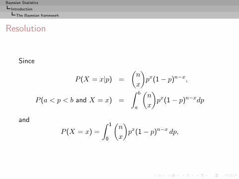
Resolution
Since
P (X = x|p) =
(n
x
)px(1 − p)n−x,
P (a < p < b and X = x) =
∫ b
a
(n
x
)px(1 − p)n−xdp
and
P (X = x) =
∫ 1
0
(n
x
)px(1 − p)n−x dp,
Bayesian Statistics
Introduction
The Bayesian framework
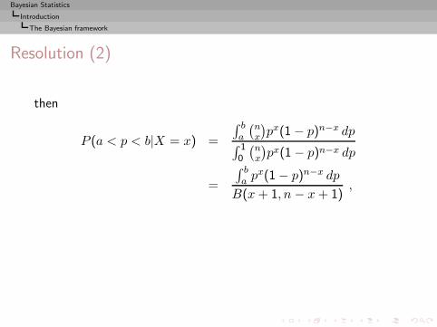
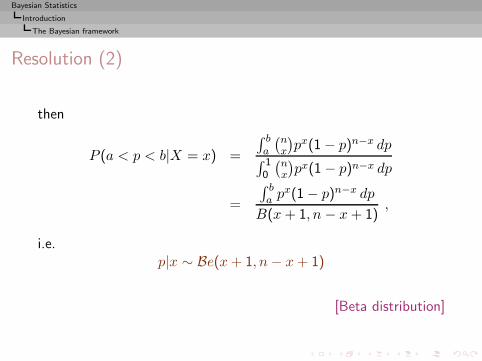
Resolution (2)
then
P (a < p < b|X = x) =
∫ ba
(nx
)px(1 − p)n−x dp
∫ 10
(nx
)px(1 − p)n−x dp
=
∫ ba p
x(1 − p)n−x dp
B(x+ 1, n − x+ 1),
Bayesian Statistics
Introduction
The Bayesian framework
Resolution (2)
then
P (a < p < b|X = x) =
∫ ba
(nx
)px(1 − p)n−x dp
∫ 10
(nx
)px(1 − p)n−x dp
=
∫ ba p
x(1 − p)n−x dp
B(x+ 1, n − x+ 1),
i.e.p|x ∼ Be(x+ 1, n− x+ 1)
[Beta distribution]
Bayesian Statistics
Introduction
Prior and posterior distributions
Prior and posterior distributions
Given f(x|θ) and π(θ), several distributions of interest:
(a) the joint distribution of (θ, x),
ϕ(θ, x) = f(x|θ)π(θ) ;
Bayesian Statistics
Introduction
Prior and posterior distributions
Prior and posterior distributions
Given f(x|θ) and π(θ), several distributions of interest:
(a) the joint distribution of (θ, x),
ϕ(θ, x) = f(x|θ)π(θ) ;
(b) the marginal distribution of x,
m(x) =
∫ϕ(θ, x) dθ
=
∫f(x|θ)π(θ) dθ ;
Bayesian Statistics
Introduction
Prior and posterior distributions
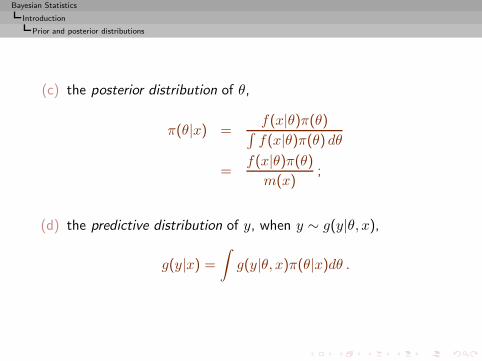
(c) the posterior distribution of θ,
π(θ|x) =f(x|θ)π(θ)∫f(x|θ)π(θ) dθ
=f(x|θ)π(θ)
m(x);
Bayesian Statistics
Introduction
Prior and posterior distributions
(c) the posterior distribution of θ,
π(θ|x) =f(x|θ)π(θ)∫f(x|θ)π(θ) dθ
=f(x|θ)π(θ)
m(x);
(d) the predictive distribution of y, when y ∼ g(y|θ, x),
g(y|x) =
∫g(y|θ, x)π(θ|x)dθ .
Bayesian Statistics
Introduction
Prior and posterior distributions
Posterior distribution
central to Bayesian inference
◮ Operates conditional upon the observation s
Bayesian Statistics
Introduction
Prior and posterior distributions
Posterior distribution
central to Bayesian inference
◮ Operates conditional upon the observation s
◮ Incorporates the requirement of the Likelihood Principle
Bayesian Statistics
Introduction
Prior and posterior distributions
Posterior distribution
central to Bayesian inference
◮ Operates conditional upon the observation s
◮ Incorporates the requirement of the Likelihood Principle
◮ Avoids averaging over the unobserved values of x
Bayesian Statistics
Introduction
Prior and posterior distributions
Posterior distribution
central to Bayesian inference
◮ Operates conditional upon the observation s
◮ Incorporates the requirement of the Likelihood Principle
◮ Avoids averaging over the unobserved values of x
◮ Coherent updating of the information available on θ,independent of the order in which i.i.d. observations arecollected
◮ Provides a complete inferential scope
Bayesian Statistics
Introduction
Prior and posterior distributions
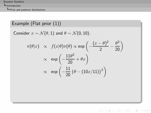
Example (Flat prior (1))
Consider x ∼ N (θ, 1) and θ ∼ N (0, 10).
π(θ|x) ∝ f(x|θ)π(θ) ∝ exp
(−(x− θ)2
2− θ2
20
)
∝ exp
(−11θ2
20+ θx
)
∝ exp
(−11
20{θ − (10x/11)}2
)
Bayesian Statistics
Introduction
Prior and posterior distributions
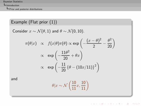
Example (Flat prior (1))
Consider x ∼ N (θ, 1) and θ ∼ N (0, 10).
π(θ|x) ∝ f(x|θ)π(θ) ∝ exp
(−(x− θ)2
2− θ2
20
)
∝ exp
(−11θ2
20+ θx
)
∝ exp
(−11
20{θ − (10x/11)}2
)
and
θ|x ∼ N(
10
11x,
10
11
)
Bayesian Statistics
Introduction
Prior and posterior distributions
Example (HPD region)
Natural confidence region
C = {θ;π(θ|x) > k}
=
{θ;
∣∣∣∣θ −10
11x
∣∣∣∣ > k′}
Bayesian Statistics
Introduction
Prior and posterior distributions
Example (HPD region)
Natural confidence region
C = {θ;π(θ|x) > k}
=
{θ;
∣∣∣∣θ −10
11x
∣∣∣∣ > k′}
Highest posterior density (HPD) region
Bayesian Statistics
Introduction
Improper prior distributions
Improper distributions
Necessary extension from a prior distribution to a prior σ-finitemeasure π such that
∫
Θπ(θ) dθ = +∞
Bayesian Statistics
Introduction
Improper prior distributions
Improper distributions
Necessary extension from a prior distribution to a prior σ-finitemeasure π such that
∫
Θπ(θ) dθ = +∞
Improper prior distribution

Bayesian Statistics
Introduction
Improper prior distributions
Justifications
Often automatic prior determination leads to improper priordistributions
1. Only way to derive a prior in noninformative settings
Bayesian Statistics
Introduction
Improper prior distributions
Justifications
Often automatic prior determination leads to improper priordistributions
1. Only way to derive a prior in noninformative settings
2. Performances of estimators derived from these generalizeddistributions usually good
Bayesian Statistics
Introduction
Improper prior distributions
Justifications
Often automatic prior determination leads to improper priordistributions
1. Only way to derive a prior in noninformative settings
2. Performances of estimators derived from these generalizeddistributions usually good
3. Improper priors often occur as limits of proper distributions
4. More robust answer against possible misspecifications of theprior
Bayesian Statistics
Introduction
Improper prior distributions
5. Generally more acceptable to non-Bayesians, with frequentistjustifications, such as:
(i) minimaxity(ii) admissibility(iii) invariance
Bayesian Statistics
Introduction
Improper prior distributions
5. Generally more acceptable to non-Bayesians, with frequentistjustifications, such as:
(i) minimaxity(ii) admissibility(iii) invariance
6. Improper priors prefered to vague proper priors such as aN (0, 1002) distribution
Bayesian Statistics
Introduction
Improper prior distributions
5. Generally more acceptable to non-Bayesians, with frequentistjustifications, such as:
(i) minimaxity(ii) admissibility(iii) invariance
6. Improper priors prefered to vague proper priors such as aN (0, 1002) distribution
7. Penalization factor in
mind
∫L(θ, d)π(θ)f(x|θ) dx dθ
Bayesian Statistics
Introduction
Improper prior distributions
Validation
Extension of the posterior distribution π(θ|x) associated with animproper prior π as given by Bayes’s formula
π(θ|x) =f(x|θ)π(θ)∫
Θ f(x|θ)π(θ) dθ,
Bayesian Statistics
Introduction
Improper prior distributions
Validation
Extension of the posterior distribution π(θ|x) associated with animproper prior π as given by Bayes’s formula
π(θ|x) =f(x|θ)π(θ)∫
Θ f(x|θ)π(θ) dθ,
when ∫
Θf(x|θ)π(θ) dθ <∞
Bayesian Statistics
Introduction
Improper prior distributions
Example
If x ∼ N (θ, 1) and π(θ) = , constant, the pseudo marginaldistribution is
m(x) =
∫ +∞
−∞
1√2π
exp{−(x− θ)2/2
}dθ =
Bayesian Statistics
Introduction
Improper prior distributions
Example
If x ∼ N (θ, 1) and π(θ) = , constant, the pseudo marginaldistribution is
m(x) =
∫ +∞
−∞
1√2π
exp{−(x− θ)2/2
}dθ =
and the posterior distribution of θ is
π(θ |x) =1√2π
exp
{−(x− θ)2
2
},
i.e., corresponds to a N (x, 1) distribution.
Bayesian Statistics
Introduction
Improper prior distributions
Example
If x ∼ N (θ, 1) and π(θ) = , constant, the pseudo marginaldistribution is
m(x) =
∫ +∞
−∞
1√2π
exp{−(x− θ)2/2
}dθ =
and the posterior distribution of θ is
π(θ |x) =1√2π
exp
{−(x− θ)2
2
},
i.e., corresponds to a N (x, 1) distribution.[independent of ω]

Bayesian Statistics
Introduction
Improper prior distributions
Warning - Warning - Warning - Warning - Warning
The mistake is to think of them [non-informative priors] asrepresenting ignorance
[Lindley, 1990]
Bayesian Statistics
Introduction
Improper prior distributions
Example (Flat prior (2))
Consider a θ ∼ N (0, τ2) prior. Then
limτ→∞
P π (θ ∈ [a, b]) = 0
for any (a, b)
Bayesian Statistics
Introduction
Improper prior distributions
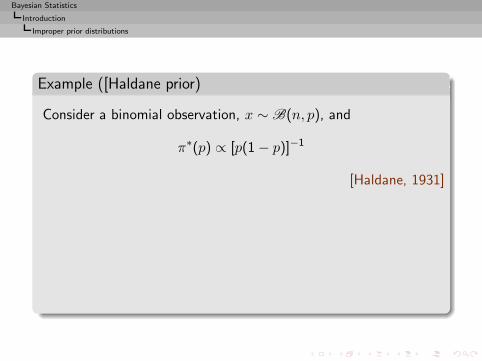
Example ([Haldane prior)
Consider a binomial observation, x ∼ B(n, p), and
π∗(p) ∝ [p(1 − p)]−1
[Haldane, 1931]
Bayesian Statistics
Introduction
Improper prior distributions
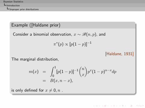
Example ([Haldane prior)
Consider a binomial observation, x ∼ B(n, p), and
π∗(p) ∝ [p(1 − p)]−1
[Haldane, 1931]The marginal distribution,
m(x) =
∫ 1
0[p(1 − p)]−1
(n
x
)px(1 − p)n−xdp
= B(x, n− x),
is only defined for x 6= 0, n .
Bayesian Statistics
Decision-Theoretic Foundations of Statistical Inference
Decision theory motivations
Introduction
Decision-Theoretic Foundations of Statistical InferenceEvaluation of estimatorsLoss functionsMinimaxity and admissibilityUsual loss functions
From Prior Information to Prior Distributions
Bayesian Point Estimation
Bayesian Calculations
Bayesian Statistics
Decision-Theoretic Foundations of Statistical Inference
Evaluation of estimators
Evaluating estimators
Purpose of most inferential studies
To provide the statistician/client with a decision d ∈ D
Bayesian Statistics
Decision-Theoretic Foundations of Statistical Inference
Evaluation of estimators
Evaluating estimators
Purpose of most inferential studies
To provide the statistician/client with a decision d ∈ D
Requires an evaluation criterion for decisions and estimators
L(θ, d)
[a.k.a. loss function]
Bayesian Statistics
Decision-Theoretic Foundations of Statistical Inference
Evaluation of estimators
Bayesian Decision Theory
Three spaces/factors:
(1) On X , distribution for the observation, f(x|θ);
Bayesian Statistics
Decision-Theoretic Foundations of Statistical Inference
Evaluation of estimators
Bayesian Decision Theory
Three spaces/factors:
(1) On X , distribution for the observation, f(x|θ);(2) On Θ, prior distribution for the parameter, π(θ);
Bayesian Statistics
Decision-Theoretic Foundations of Statistical Inference
Evaluation of estimators
Bayesian Decision Theory
Three spaces/factors:
(1) On X , distribution for the observation, f(x|θ);(2) On Θ, prior distribution for the parameter, π(θ);
(3) On Θ×D , loss function associated with the decisions, L(θ, δ);
Bayesian Statistics
Decision-Theoretic Foundations of Statistical Inference
Evaluation of estimators
Foundations
Theorem (Existence)
There exists an axiomatic derivation of the existence of aloss function.
[DeGroot, 1970]
Bayesian Statistics
Decision-Theoretic Foundations of Statistical Inference
Loss functions
Estimators
Decision procedure δ usually called estimator(while its value δ(x) called estimate of θ)
Bayesian Statistics
Decision-Theoretic Foundations of Statistical Inference
Loss functions
Estimators
Decision procedure δ usually called estimator(while its value δ(x) called estimate of θ)
Fact
Impossible to uniformly minimize (in d) the loss function
L(θ, d)
when θ is unknown
Bayesian Statistics
Decision-Theoretic Foundations of Statistical Inference
Loss functions
Frequentist Principle
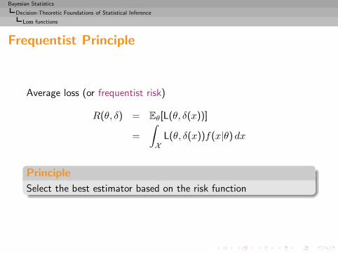
Average loss (or frequentist risk)
R(θ, δ) = Eθ[L(θ, δ(x))]
=
∫
XL(θ, δ(x))f(x|θ) dx
Bayesian Statistics
Decision-Theoretic Foundations of Statistical Inference
Loss functions
Frequentist Principle
Average loss (or frequentist risk)
R(θ, δ) = Eθ[L(θ, δ(x))]
=
∫
XL(θ, δ(x))f(x|θ) dx
Principle
Select the best estimator based on the risk function
Bayesian Statistics
Decision-Theoretic Foundations of Statistical Inference
Loss functions
Difficulties with frequentist paradigm
(1) Error averaged over the different values of x proportionally tothe density f(x|θ): not so appealing for a client, who wantsoptimal results for her data x!
Bayesian Statistics
Decision-Theoretic Foundations of Statistical Inference
Loss functions
Difficulties with frequentist paradigm
(1) Error averaged over the different values of x proportionally tothe density f(x|θ): not so appealing for a client, who wantsoptimal results for her data x!
(2) Assumption of repeatability of experiments not alwaysgrounded.
(3) R(θ, δ) is a function of θ: there is no total ordering on the setof procedures.
Bayesian Statistics
Decision-Theoretic Foundations of Statistical Inference
Loss functions
Bayesian principle
Principle Integrate over the space Θ to get the posterior expectedloss
ρ(π, d|x) = Eπ[L(θ, d)|x]
=
∫
ΘL(θ, d)π(θ|x) dθ,
Bayesian Statistics
Decision-Theoretic Foundations of Statistical Inference
Loss functions
Bayesian principle (2)
Alternative
Integrate over the space Θ and compute integrated risk
r(π, δ) = Eπ[R(θ, δ)]
=
∫
Θ
∫
XL(θ, δ(x)) f(x|θ) dx π(θ) dθ
which induces a total ordering on estimators.
Bayesian Statistics
Decision-Theoretic Foundations of Statistical Inference
Loss functions
Bayesian principle (2)
Alternative
Integrate over the space Θ and compute integrated risk
r(π, δ) = Eπ[R(θ, δ)]
=
∫
Θ
∫
XL(θ, δ(x)) f(x|θ) dx π(θ) dθ
which induces a total ordering on estimators.
Existence of an optimal decision
Bayesian Statistics
Decision-Theoretic Foundations of Statistical Inference
Loss functions
Bayes estimator
Theorem (Construction of Bayes estimators)
An estimator minimizingr(π, δ)
can be obtained by selecting, for every x ∈ X , the value δ(x)which minimizes
ρ(π, δ|x)since
r(π, δ) =
∫
Xρ(π, δ(x)|x)m(x) dx.
Both approaches give the same estimator
Bayesian Statistics
Decision-Theoretic Foundations of Statistical Inference
Loss functions
Bayes estimator (2)
Definition (Bayes optimal procedure)
A Bayes estimator associated with a prior distribution π and a lossfunction L is
arg minδr(π, δ)
The value r(π) = r(π, δπ) is called the Bayes risk
Bayesian Statistics
Decision-Theoretic Foundations of Statistical Inference
Loss functions
Infinite Bayes risk
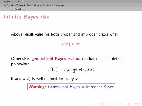
Above result valid for both proper and improper priors when
r(π) <∞
Bayesian Statistics
Decision-Theoretic Foundations of Statistical Inference
Loss functions
Infinite Bayes risk
Above result valid for both proper and improper priors when
r(π) <∞
Otherwise, generalized Bayes estimator that must be definedpointwise:
δπ(x) = arg mind
ρ(π, d|x)
if ρ(π, d|x) is well-defined for every x.
Warning: Generalized Bayes 6= Improper Bayes

Bayesian Statistics
Decision-Theoretic Foundations of Statistical Inference
Minimaxity and admissibility
Minimaxity
Frequentist insurance against the worst case and (weak) totalordering on D∗
Bayesian Statistics
Decision-Theoretic Foundations of Statistical Inference
Minimaxity and admissibility
Minimaxity
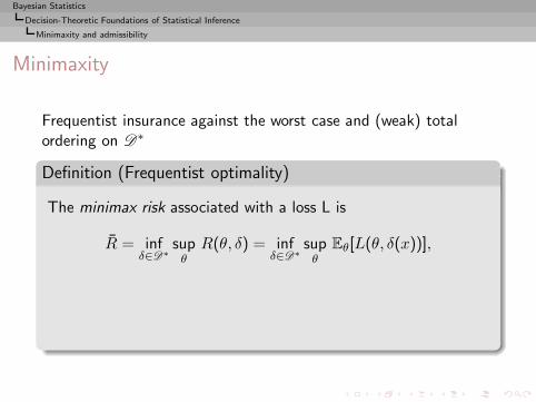
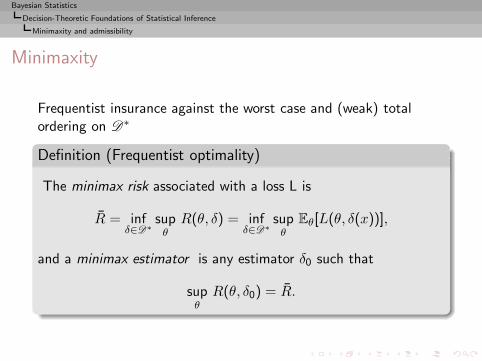
Frequentist insurance against the worst case and (weak) totalordering on D∗
Definition (Frequentist optimality)
The minimax risk associated with a loss L is
R = infδ∈D∗
supθR(θ, δ) = inf
δ∈D∗supθ
Eθ[L(θ, δ(x))],
Bayesian Statistics
Decision-Theoretic Foundations of Statistical Inference
Minimaxity and admissibility
Minimaxity
Frequentist insurance against the worst case and (weak) totalordering on D∗
Definition (Frequentist optimality)
The minimax risk associated with a loss L is
R = infδ∈D∗
supθR(θ, δ) = inf
δ∈D∗supθ
Eθ[L(θ, δ(x))],
and a minimax estimator is any estimator δ0 such that
supθR(θ, δ0) = R.

Bayesian Statistics
Decision-Theoretic Foundations of Statistical Inference
Minimaxity and admissibility
Criticisms
◮ Analysis in terms of the worst case

Bayesian Statistics
Decision-Theoretic Foundations of Statistical Inference
Minimaxity and admissibility
Criticisms
◮ Analysis in terms of the worst case
◮ Does not incorporate prior information

Bayesian Statistics
Decision-Theoretic Foundations of Statistical Inference
Minimaxity and admissibility
Criticisms
◮ Analysis in terms of the worst case
◮ Does not incorporate prior information
◮ Too conservative

Bayesian Statistics
Decision-Theoretic Foundations of Statistical Inference
Minimaxity and admissibility
Criticisms
◮ Analysis in terms of the worst case
◮ Does not incorporate prior information
◮ Too conservative
◮ Difficult to exhibit/construct
Bayesian Statistics
Decision-Theoretic Foundations of Statistical Inference
Minimaxity and admissibility
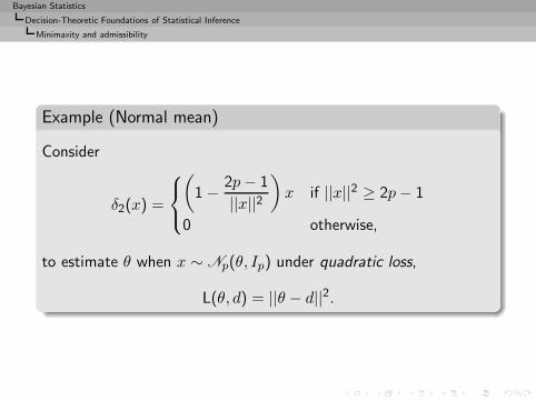
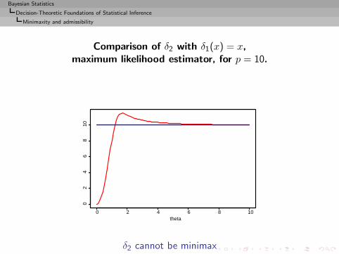
Example (Normal mean)
Consider
δ2(x) =
(1 − 2p− 1
||x||2)x if ||x||2 ≥ 2p− 1
0 otherwise,
to estimate θ when x ∼ Np(θ, Ip) under quadratic loss,
L(θ, d) = ||θ − d||2.
Bayesian Statistics
Decision-Theoretic Foundations of Statistical Inference
Minimaxity and admissibility
Comparison of δ2 with δ1(x) = x,maximum likelihood estimator, for p = 10.
0 2 4 6 8 10
02
46
810
theta
δ2 cannot be minimax
Bayesian Statistics
Decision-Theoretic Foundations of Statistical Inference
Minimaxity and admissibility
Minimaxity (2)
Existence
If D ⊂ Rk convex and compact, and if L(θ, d) continuous andconvex as a function of d for every θ ∈ Θ, there exists anonrandomized minimax estimator.
Bayesian Statistics
Decision-Theoretic Foundations of Statistical Inference
Minimaxity and admissibility
Connection with Bayesian approach
The Bayes risks are always smaller than the minimax risk:
r = supπr(π) = sup
πinfδ∈D
r(π, δ) ≤ r = infδ∈D∗
supθR(θ, δ).
Bayesian Statistics
Decision-Theoretic Foundations of Statistical Inference
Minimaxity and admissibility
Connection with Bayesian approach
The Bayes risks are always smaller than the minimax risk:
r = supπr(π) = sup
πinfδ∈D
r(π, δ) ≤ r = infδ∈D∗
supθR(θ, δ).
Definition
The estimation problem has a value when r = r, i.e.
supπ
infδ∈D
r(π, δ) = infδ∈D∗
supθR(θ, δ).
r is the maximin risk and the corresponding π the favourable prior
Bayesian Statistics
Decision-Theoretic Foundations of Statistical Inference
Minimaxity and admissibility
Maximin-ity
When the problem has a value, some minimax estimators are Bayesestimators for the least favourable distributions.
Bayesian Statistics
Decision-Theoretic Foundations of Statistical Inference
Minimaxity and admissibility
Maximin-ity (2)
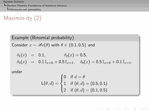
Example (Binomial probability)
Consider x ∼ Be(θ) with θ ∈ {0.1, 0.5} and
δ1(x) = 0.1, δ2(x) = 0.5,
δ3(x) = 0.1 Ix=0 + 0.5 Ix=1, δ4(x) = 0.5 Ix=0 + 0.1 Ix=1.
under
L(θ, d) =
0 if d = θ
1 if (θ, d) = (0.5, 0.1)
2 if (θ, d) = (0.1, 0.5)
Bayesian Statistics
Decision-Theoretic Foundations of Statistical Inference
Minimaxity and admissibility
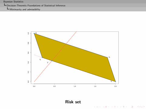
0.0 0.5 1.0 1.5 2.0
0.0
0.2
0.4
0.6
0.8
1.0
δ2
δ4
δ1
δ3
δ*
Risk set
Bayesian Statistics
Decision-Theoretic Foundations of Statistical Inference
Minimaxity and admissibility
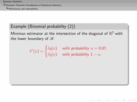
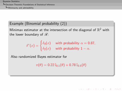
Example (Binomial probability (2))
Minimax estimator at the intersection of the diagonal of R2 withthe lower boundary of R:
δ∗(x) =
{δ3(x) with probability α = 0.87,
δ2(x) with probability 1 − α.
Bayesian Statistics
Decision-Theoretic Foundations of Statistical Inference
Minimaxity and admissibility
Example (Binomial probability (2))
Minimax estimator at the intersection of the diagonal of R2 withthe lower boundary of R:
δ∗(x) =
{δ3(x) with probability α = 0.87,
δ2(x) with probability 1 − α.
Also randomized Bayes estimator for
π(θ) = 0.22 I0.1(θ) + 0.78 I0.5(θ)
Bayesian Statistics
Decision-Theoretic Foundations of Statistical Inference
Minimaxity and admissibility
Checking minimaxity
Theorem (Bayes & minimax)
If δ0 is a Bayes estimator for π0 and if
R(θ, δ0) ≤ r(π0)
for every θ in the support of π0, then δ0 is minimax and π0 is theleast favourable distribution
Bayesian Statistics
Decision-Theoretic Foundations of Statistical Inference
Minimaxity and admissibility
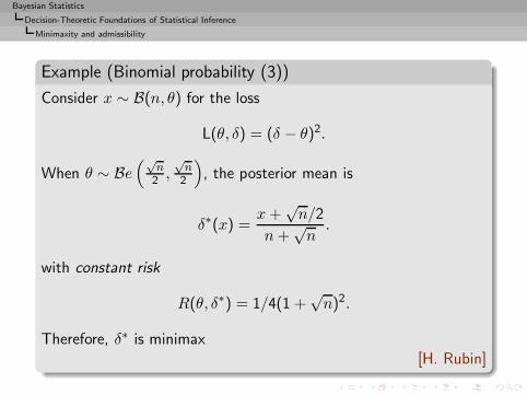
Example (Binomial probability (3))
Consider x ∼ B(n, θ) for the loss
L(θ, δ) = (δ − θ)2.
When θ ∼ Be(√
n2 ,
√n
2
), the posterior mean is
δ∗(x) =x+
√n/2
n+√n.
with constant risk
R(θ, δ∗) = 1/4(1 +√n)2.
Therefore, δ∗ is minimax[H. Rubin]
Bayesian Statistics
Decision-Theoretic Foundations of Statistical Inference
Minimaxity and admissibility
Checking minimaxity (2)
Theorem (Bayes & minimax (2))
If for a sequence (πn) of proper priors, the generalised Bayesestimator δ0 satisfies
R(θ, δ0) ≤ limn→∞
r(πn) < +∞
for every θ ∈ Θ, then δ0 is minimax.
Bayesian Statistics
Decision-Theoretic Foundations of Statistical Inference
Minimaxity and admissibility
Example (Normal mean)
When x ∼ N (θ, 1),δ0(x) = x
is a generalised Bayes estimator associated with
π(θ) ∝ 1
Bayesian Statistics
Decision-Theoretic Foundations of Statistical Inference
Minimaxity and admissibility
Example (Normal mean)
When x ∼ N (θ, 1),δ0(x) = x
is a generalised Bayes estimator associated with
π(θ) ∝ 1
Since, for πn(θ) = exp{−θ2/2n},
R(δ0, θ) = Eθ[(x− θ)2
]= 1
= limn→∞
r(πn) = limn→∞
n
n+ 1
δ0 is minimax.
Bayesian Statistics
Decision-Theoretic Foundations of Statistical Inference
Minimaxity and admissibility
Admissibility
Reduction of the set of acceptable estimators based on “local”properties
Definition (Admissible estimator)
An estimator δ0 is inadmissible if there exists an estimator δ1 suchthat, for every θ,
R(θ, δ0) ≥ R(θ, δ1)
and, for at least one θ0
R(θ0, δ0) > R(θ0, δ1)
Otherwise, δ0 is admissible
Bayesian Statistics
Decision-Theoretic Foundations of Statistical Inference
Minimaxity and admissibility
Minimaxity & admissibility
If there exists a unique minimax estimator, this estimator isadmissible.
The converse is false!
Bayesian Statistics
Decision-Theoretic Foundations of Statistical Inference
Minimaxity and admissibility
Minimaxity & admissibility
If there exists a unique minimax estimator, this estimator isadmissible.
The converse is false!
If δ0 is admissible with constant risk, δ0 is the unique minimaxestimator.
The converse is false!
Bayesian Statistics
Decision-Theoretic Foundations of Statistical Inference
Minimaxity and admissibility
The Bayesian perspective
Admissibility strongly related to the Bayes paradigm: Bayesestimators often constitute the class of admissible estimators
Bayesian Statistics
Decision-Theoretic Foundations of Statistical Inference
Minimaxity and admissibility
The Bayesian perspective
Admissibility strongly related to the Bayes paradigm: Bayesestimators often constitute the class of admissible estimators
◮ If π is strictly positive on Θ, with
r(π) =
∫
ΘR(θ, δπ)π(θ) dθ <∞
and R(θ, δ), is continuous, then the Bayes estimator δπ isadmissible.
◮ If the Bayes estimator associated with a prior π is unique, it isadmissible.
Regular (6=generalized) Bayes estimators always admissible
Bayesian Statistics
Decision-Theoretic Foundations of Statistical Inference
Minimaxity and admissibility
Example (Normal mean)
Consider x ∼ N (θ, 1) and the test of H0 : θ ≤ 0, i.e. theestimation of
IH0(θ)
Bayesian Statistics
Decision-Theoretic Foundations of Statistical Inference
Minimaxity and admissibility
Example (Normal mean)
Consider x ∼ N (θ, 1) and the test of H0 : θ ≤ 0, i.e. theestimation of
IH0(θ)
Under the loss(IH0(θ) − δ(x))2 ,
the estimator (p-value)
p(x) = P0(X > x) (X ∼ N (0, 1))
= 1 − Φ(x),
is Bayes under Lebesgue measure.
Bayesian Statistics
Decision-Theoretic Foundations of Statistical Inference
Minimaxity and admissibility
Example (Normal mean (2))
Indeed
p(x) = Eπ[IH0(θ)|x] = P π(θ < 0|x)
= P π(θ − x < −x|x) = 1 − Φ(x).
The Bayes risk of p is finite and p(s) is admissible.
Bayesian Statistics
Decision-Theoretic Foundations of Statistical Inference
Minimaxity and admissibility
Example (Normal mean (3))
Consider x ∼ N (θ, 1). Then δ0(x) = x is a generalised Bayesestimator, is admissible, but
r(π, δ0) =
∫ +∞
−∞R(θ, δ0) dθ
=
∫ +∞
−∞1 dθ = +∞.
Bayesian Statistics
Decision-Theoretic Foundations of Statistical Inference
Minimaxity and admissibility
Example (Normal mean (4))
Consider x ∼ Np(θ, Ip). If
L(θ, d) = (d− ||θ||2)2
the Bayes estimator for the Lebesgue measure is
δπ(x) = ||x||2 + p.
This estimator is not admissible because it is dominated by
δ0(x) = ||x||2 − p
Bayesian Statistics
Decision-Theoretic Foundations of Statistical Inference
Usual loss functions
The quadratic loss
Historically, first loss function (Legendre, Gauss)
L(θ, d) = (θ − d)2
Bayesian Statistics
Decision-Theoretic Foundations of Statistical Inference
Usual loss functions
The quadratic loss
Historically, first loss function (Legendre, Gauss)
L(θ, d) = (θ − d)2
orL(θ, d) = ||θ − d||2
Bayesian Statistics
Decision-Theoretic Foundations of Statistical Inference
Usual loss functions
Proper loss
Posterior mean
The Bayes estimator δπ associated with the prior π and with thequadratic loss is the posterior expectation
δπ(x) = Eπ[θ|x] =
∫Θ θf(x|θ)π(θ) dθ∫Θ f(x|θ)π(θ) dθ
.
Bayesian Statistics
Decision-Theoretic Foundations of Statistical Inference
Usual loss functions
The absolute error loss
Alternatives to the quadratic loss:
L(θ, d) = | θ − d | ,
or
Lk1,k2(θ, d) =
{k2(θ − d) if θ > d,
k1(d− θ) otherwise.(1)
Bayesian Statistics
Decision-Theoretic Foundations of Statistical Inference
Usual loss functions
The absolute error loss
Alternatives to the quadratic loss:
L(θ, d) = | θ − d | ,
or
Lk1,k2(θ, d) =
{k2(θ − d) if θ > d,
k1(d− θ) otherwise.(1)
L1 estimator
The Bayes estimator associated with π and (1) is a (k2/(k1 + k2))fractile of π(θ|x).
Bayesian Statistics
Decision-Theoretic Foundations of Statistical Inference
Usual loss functions
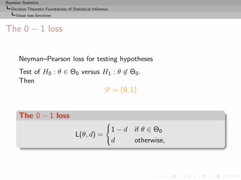
The 0 − 1 loss
Neyman–Pearson loss for testing hypotheses
Test of H0 : θ ∈ Θ0 versus H1 : θ 6∈ Θ0.Then
D = {0, 1}
Bayesian Statistics
Decision-Theoretic Foundations of Statistical Inference
Usual loss functions
The 0 − 1 loss
Neyman–Pearson loss for testing hypotheses
Test of H0 : θ ∈ Θ0 versus H1 : θ 6∈ Θ0.Then
D = {0, 1}
The 0 − 1 loss
L(θ, d) =
{1 − d if θ ∈ Θ0
d otherwise,
Bayesian Statistics
Decision-Theoretic Foundations of Statistical Inference
Usual loss functions
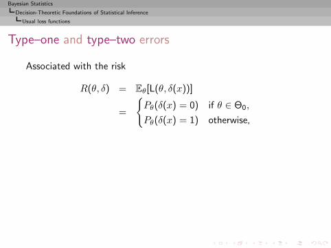
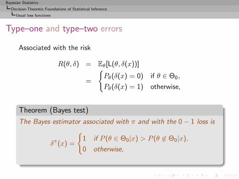
Type–one and type–two errors
Associated with the risk
R(θ, δ) = Eθ[L(θ, δ(x))]
=
{Pθ(δ(x) = 0) if θ ∈ Θ0,
Pθ(δ(x) = 1) otherwise,
Bayesian Statistics
Decision-Theoretic Foundations of Statistical Inference
Usual loss functions
Type–one and type–two errors
Associated with the risk
R(θ, δ) = Eθ[L(θ, δ(x))]
=
{Pθ(δ(x) = 0) if θ ∈ Θ0,
Pθ(δ(x) = 1) otherwise,
Theorem (Bayes test)
The Bayes estimator associated with π and with the 0 − 1 loss is
δπ(x) =
{1 if P (θ ∈ Θ0|x) > P (θ 6∈ Θ0|x),0 otherwise,
Bayesian Statistics
Decision-Theoretic Foundations of Statistical Inference
Usual loss functions
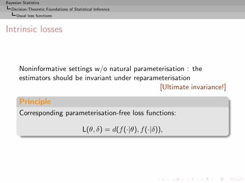
Intrinsic losses
Noninformative settings w/o natural parameterisation : theestimators should be invariant under reparameterisation
[Ultimate invariance!]
Principle
Corresponding parameterisation-free loss functions:
L(θ, δ) = d(f(·|θ), f(·|δ)),
Bayesian Statistics
Decision-Theoretic Foundations of Statistical Inference
Usual loss functions
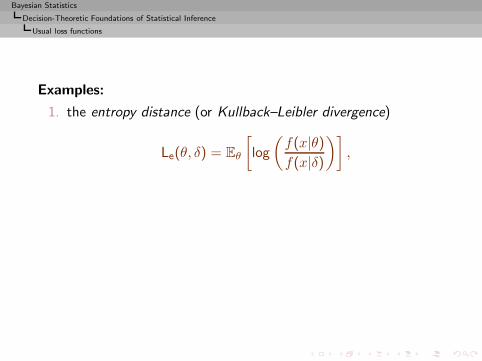
Examples:
1. the entropy distance (or Kullback–Leibler divergence)
Le(θ, δ) = Eθ
[log
(f(x|θ)f(x|δ)
)],
Bayesian Statistics
Decision-Theoretic Foundations of Statistical Inference
Usual loss functions
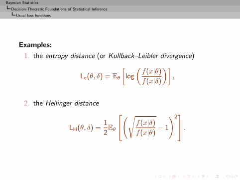
Examples:
1. the entropy distance (or Kullback–Leibler divergence)
Le(θ, δ) = Eθ
[log
(f(x|θ)f(x|δ)
)],
2. the Hellinger distance
LH(θ, δ) =1
2Eθ
(√
f(x|δ)f(x|θ) − 1
)2
.
Bayesian Statistics
Decision-Theoretic Foundations of Statistical Inference
Usual loss functions
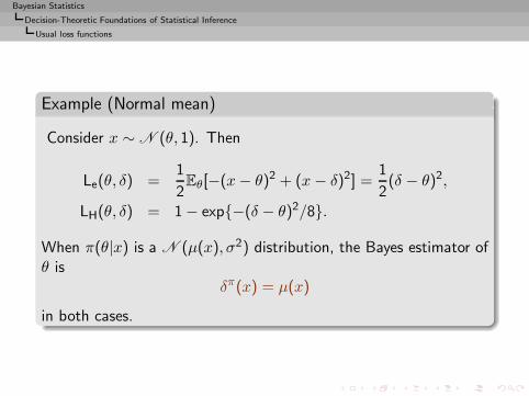
Example (Normal mean)
Consider x ∼ N (θ, 1). Then
Le(θ, δ) =1
2Eθ[−(x− θ)2 + (x− δ)2] =
1
2(δ − θ)2,
LH(θ, δ) = 1 − exp{−(δ − θ)2/8}.
When π(θ|x) is a N (µ(x), σ2) distribution, the Bayes estimator ofθ is
δπ(x) = µ(x)
in both cases.
Bayesian Statistics
From Prior Information to Prior Distributions
From prior information to prior distributions
Introduction
Decision-Theoretic Foundations of Statistical Inference
From Prior Information to Prior DistributionsModelsSubjective determinationConjugate priorsNoninformative prior distributions
Bayesian Point Estimation
Bayesian Calculations
Bayesian Statistics
From Prior Information to Prior Distributions
Models
Prior Distributions
The most critical and most criticized point of Bayesian analysis !Because...
the prior distribution is the key to Bayesian inference

Bayesian Statistics
From Prior Information to Prior Distributions
Models
But...
In practice, it seldom occurs that the available prior information isprecise enough to lead to an exact determination of the priordistribution
There is no such thing as the prior distribution!

Bayesian Statistics
From Prior Information to Prior Distributions
Models
Rather...
The prior is a tool summarizing available information as well asuncertainty related with this information,And...Ungrounded prior distributions produce unjustified posteriorinference
Bayesian Statistics
From Prior Information to Prior Distributions
Subjective determination
Subjective priors
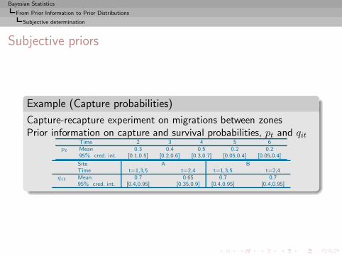
Example (Capture probabilities)
Capture-recapture experiment on migrations between zonesPrior information on capture and survival probabilities, pt and qit
Time 2 3 4 5 6pt Mean 0.3 0.4 0.5 0.2 0.2
95% cred. int. [0.1,0.5] [0.2,0.6] [0.3,0.7] [0.05,0.4] [0.05,0.4]
Site A BTime t=1,3,5 t=2,4 t=1,3,5 t=2,4
qit Mean 0.7 0.65 0.7 0.795% cred. int. [0.4,0.95] [0.35,0.9] [0.4,0.95] [0.4,0.95]
Bayesian Statistics
From Prior Information to Prior Distributions
Subjective determination
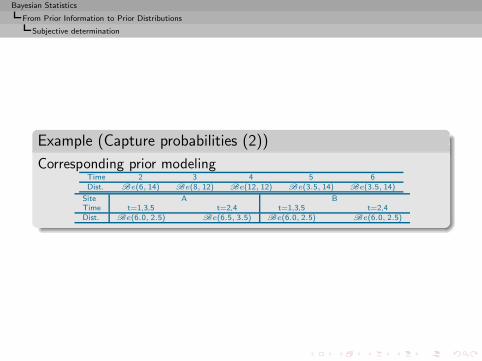
Example (Capture probabilities (2))
Corresponding prior modelingTime 2 3 4 5 6Dist. Be(6, 14) Be(8, 12) Be(12, 12) Be(3.5, 14) Be(3.5, 14)
Site A BTime t=1,3,5 t=2,4 t=1,3,5 t=2,4Dist. Be(6.0, 2.5) Be(6.5, 3.5) Be(6.0, 2.5) Be(6.0, 2.5)

Bayesian Statistics
From Prior Information to Prior Distributions
Subjective determination
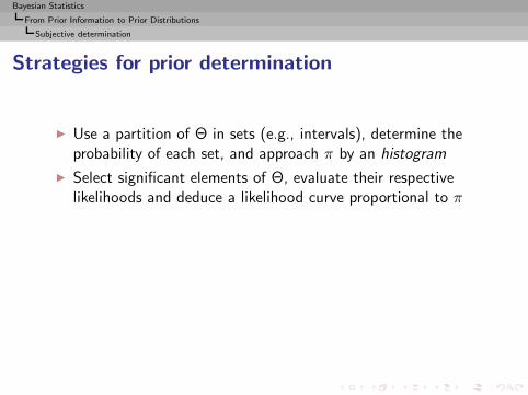
Strategies for prior determination
◮ Use a partition of Θ in sets (e.g., intervals), determine theprobability of each set, and approach π by an histogram
Bayesian Statistics
From Prior Information to Prior Distributions
Subjective determination
Strategies for prior determination
◮ Use a partition of Θ in sets (e.g., intervals), determine theprobability of each set, and approach π by an histogram
◮ Select significant elements of Θ, evaluate their respectivelikelihoods and deduce a likelihood curve proportional to π
◮ Use the marginal distribution of x,
m(x) =
∫
Θf(x|θ)π(θ) dθ
◮ Empirical and hierarchical Bayes techniques
Bayesian Statistics
From Prior Information to Prior Distributions
Subjective determination
◮ Select a maximum entropy prior when prior characteristicsare known:
Eπ[gk(θ)] = ωk (k = 1, . . . ,K)
with solution, in the discrete case
π∗(θi) =exp
{∑K1 λkgk(θi)
}
∑j exp
{∑K1 λkgk(θj)
} ,
and, in the continuous case,
π∗(θ) =exp
{∑K1 λkgk(θ)
}π0(θ)
∫exp
{∑K1 λkgk(η)
}π0(dη)
,
the λk’s being Lagrange multipliers and π0 a referencemeasure [Caveat]
Bayesian Statistics
From Prior Information to Prior Distributions
Subjective determination
◮ Parametric approximationsRestrict choice of π to a parameterised density
π(θ|λ)
and determine the corresponding (hyper-)parameters
λ
through the moments or quantiles of π
Bayesian Statistics
From Prior Information to Prior Distributions
Subjective determination
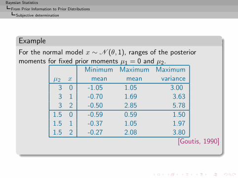
Example
For the normal model x ∼ N (θ, 1), ranges of the posteriormoments for fixed prior moments µ1 = 0 and µ2.
Minimum Maximum Maximumµ2 x mean mean variance
3 0 -1.05 1.05 3.003 1 -0.70 1.69 3.633 2 -0.50 2.85 5.78
1.5 0 -0.59 0.59 1.501.5 1 -0.37 1.05 1.971.5 2 -0.27 2.08 3.80
[Goutis, 1990]
Bayesian Statistics
From Prior Information to Prior Distributions
Conjugate priors
Conjugate priors
Specific parametric family with analytical properties
Definition
A family F of probability distributions on Θ is conjugate for alikelihood function f(x|θ) if, for every π ∈ F , the posteriordistribution π(θ|x) also belongs to F .
[Raiffa & Schlaifer, 1961]Only of interest when F is parameterised : switching from prior toposterior distribution is reduced to an updating of thecorresponding parameters.

Bayesian Statistics
From Prior Information to Prior Distributions
Conjugate priors
Justifications
◮ Limited/finite information conveyed by x
Bayesian Statistics
From Prior Information to Prior Distributions
Conjugate priors
Justifications
◮ Limited/finite information conveyed by x
◮ Preservation of the structure of π(θ)
Bayesian Statistics
From Prior Information to Prior Distributions
Conjugate priors
Justifications
◮ Limited/finite information conveyed by x
◮ Preservation of the structure of π(θ)
◮ Exchangeability motivations
Bayesian Statistics
From Prior Information to Prior Distributions
Conjugate priors
Justifications
◮ Limited/finite information conveyed by x
◮ Preservation of the structure of π(θ)
◮ Exchangeability motivations
◮ Device of virtual past observations
Bayesian Statistics
From Prior Information to Prior Distributions
Conjugate priors
Justifications
◮ Limited/finite information conveyed by x
◮ Preservation of the structure of π(θ)
◮ Exchangeability motivations
◮ Device of virtual past observations
◮ Linearity of some estimators
Bayesian Statistics
From Prior Information to Prior Distributions
Conjugate priors
Justifications
◮ Limited/finite information conveyed by x
◮ Preservation of the structure of π(θ)
◮ Exchangeability motivations
◮ Device of virtual past observations
◮ Linearity of some estimators
◮ Tractability and simplicity
◮ First approximations to adequate priors, backed up byrobustness analysis
Bayesian Statistics
From Prior Information to Prior Distributions
Conjugate priors
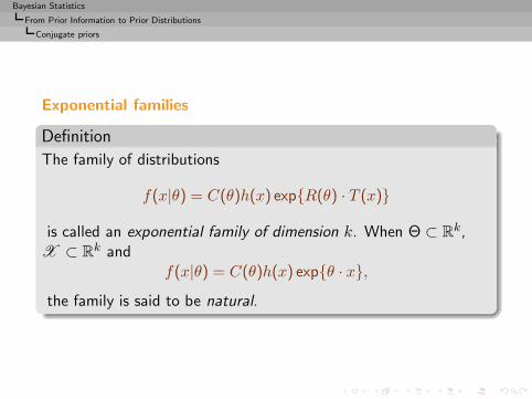
Exponential families
Definition
The family of distributions
f(x|θ) = C(θ)h(x) exp{R(θ) · T (x)}
is called an exponential family of dimension k. When Θ ⊂ Rk,X ⊂ Rk and
f(x|θ) = C(θ)h(x) exp{θ · x},the family is said to be natural.
Bayesian Statistics
From Prior Information to Prior Distributions
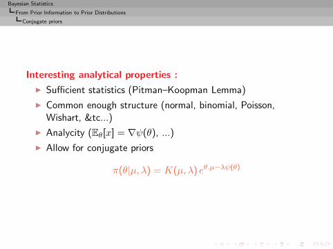
Conjugate priors
Interesting analytical properties :
◮ Sufficient statistics (Pitman–Koopman Lemma)
◮ Common enough structure (normal, binomial, Poisson,Wishart, &tc...)
◮ Analycity (Eθ[x] = ∇ψ(θ), ...)
◮ Allow for conjugate priors
π(θ|µ, λ) = K(µ, λ) eθ.µ−λψ(θ)
Bayesian Statistics
From Prior Information to Prior Distributions
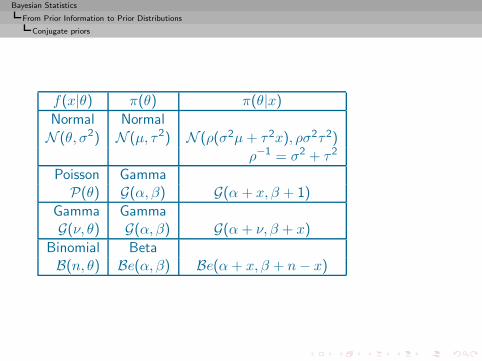
Conjugate priors
f(x|θ) π(θ) π(θ|x)Normal Normal
N (θ, σ2) N (µ, τ2) N (ρ(σ2µ+ τ2x), ρσ2τ2)
ρ−1 = σ2 + τ2
Poisson GammaP(θ) G(α, β) G(α + x, β + 1)
Gamma GammaG(ν, θ) G(α, β) G(α+ ν, β + x)
Binomial BetaB(n, θ) Be(α, β) Be(α+ x, β + n− x)
Bayesian Statistics
From Prior Information to Prior Distributions
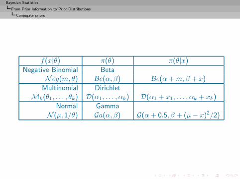
Conjugate priors
f(x|θ) π(θ) π(θ|x)Negative Binomial Beta
N eg(m, θ) Be(α, β) Be(α+m,β + x)
Multinomial DirichletMk(θ1, . . . , θk) D(α1, . . . , αk) D(α1 + x1, . . . , αk + xk)
Normal Gamma
N (µ, 1/θ) Ga(α, β) G(α + 0.5, β + (µ− x)2/2)
Bayesian Statistics
From Prior Information to Prior Distributions
Conjugate priors
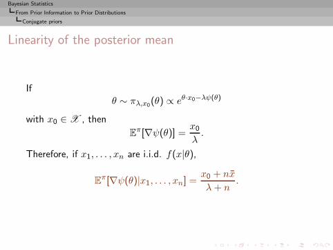
Linearity of the posterior mean
Ifθ ∼ πλ,x0
(θ) ∝ eθ·x0−λψ(θ)
with x0 ∈ X , then
Eπ[∇ψ(θ)] =
x0
λ.
Therefore, if x1, . . . , xn are i.i.d. f(x|θ),
Eπ[∇ψ(θ)|x1, . . . , xn] =
x0 + nx
λ+ n.
Bayesian Statistics
From Prior Information to Prior Distributions
Conjugate priors
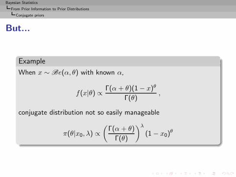
But...
Example
When x ∼ Be(α, θ) with known α,
f(x|θ) ∝ Γ(α + θ)(1 − x)θ
Γ(θ),
conjugate distribution not so easily manageable
π(θ|x0, λ) ∝(
Γ(α + θ)
Γ(θ)
)λ(1 − x0)
θ
Bayesian Statistics
From Prior Information to Prior Distributions
Conjugate priors
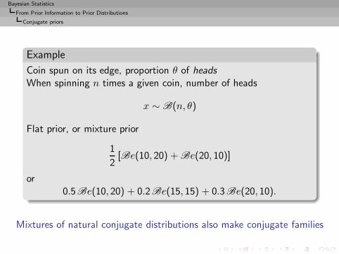
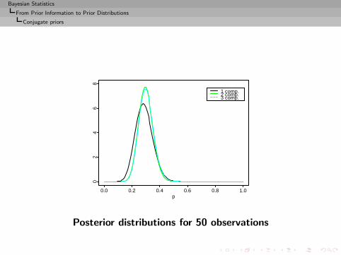
Example
Coin spun on its edge, proportion θ of headsWhen spinning n times a given coin, number of heads
x ∼ B(n, θ)
Flat prior, or mixture prior
1
2[Be(10, 20) + Be(20, 10)]
or0.5Be(10, 20) + 0.2Be(15, 15) + 0.3Be(20, 10).
Mixtures of natural conjugate distributions also make conjugate families
Bayesian Statistics
From Prior Information to Prior Distributions
Conjugate priors
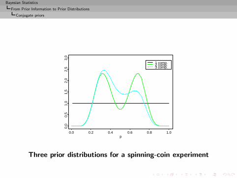
p0.0 0.2 0.4 0.6 0.8 1.0
0.0
0.5
1.0
1.5
2.0
2.5
3.0
1 comp.2 comp.3 comp.
Three prior distributions for a spinning-coin experiment
Bayesian Statistics
From Prior Information to Prior Distributions
Conjugate priors
p0.0 0.2 0.4 0.6 0.8 1.0
02
46
81 comp.2 comp.3 comp.
Posterior distributions for 50 observations

Bayesian Statistics
From Prior Information to Prior Distributions
Conjugate priors
What if all we know is that we know “nothing” ?!
In the absence of prior information, prior distributions solelyderived from the sample distribution f(x|θ)
[Noninformative priors]

Bayesian Statistics
From Prior Information to Prior Distributions
Conjugate priors
Re-Warning
Noninformative priors cannot be expected to representexactly total ignorance about the problem at hand, butshould rather be taken as reference or default priors,upon which everyone could fall back when the priorinformation is missing.
[Kass and Wasserman, 1996]
Bayesian Statistics
From Prior Information to Prior Distributions
Conjugate priors
Laplace’s prior
Principle of Insufficient Reason (Laplace)
Θ = {θ1, · · · , θp} π(θi) = 1/p
Extension to continuous spaces
π(θ) ∝ 1
Bayesian Statistics
From Prior Information to Prior Distributions
Conjugate priors
◮ Lack of reparameterization invariance/coherence
ψ = eθ π1(ψ) =1
ψ6= π2(ψ) = 1
◮ Problems of properness
x ∼ N (θ, σ2), π(θ, σ) = 1
π(θ, σ|x) ∝ e−(x−θ)2/2σ2σ−1
⇒ π(σ|x) ∝ 1 (!!!)
Bayesian Statistics
From Prior Information to Prior Distributions
Conjugate priors
Invariant priors
Principle: Agree with the natural symmetries of the problem
- Identify invariance structures as group action
G : x→ g(x) ∼ f(g(x)|g(θ))G : θ → g(θ)G∗ : L(d, θ) = L(g∗(d), g(θ))
- Determine an invariant prior
π(g(A)) = π(A)

Bayesian Statistics
From Prior Information to Prior Distributions
Conjugate priors
Solution: Right Haar measureBut...
◮ Requires invariance to be part of the decision problem
◮ Missing in most discrete setups (Poisson)

Bayesian Statistics
From Prior Information to Prior Distributions
Conjugate priors
The Jeffreys prior
Based on Fisher information
I(θ) = Eθ
[∂ℓ
∂θt∂ℓ
∂θ
]
The Jeffreys prior distribution is
π∗(θ) ∝ |I(θ)|1/2
Bayesian Statistics
From Prior Information to Prior Distributions
Conjugate priors
Pros & Cons
◮ Relates to information theory
◮ Agrees with most invariant priors
◮ Parameterization invariant
◮ Suffers from dimensionality curse
◮ Not coherent for Likelihood Principle
Bayesian Statistics
From Prior Information to Prior Distributions
Conjugate priors
Example
x ∼ Np(θ, Ip), η = ‖θ‖2, π(η) = ηp/2−1
Eπ[η|x] = ‖x‖2 + p Bias 2p
Bayesian Statistics
From Prior Information to Prior Distributions
Conjugate priors
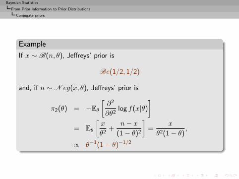
Example
If x ∼ B(n, θ), Jeffreys’ prior is
Be(1/2, 1/2)
and, if n ∼ N eg(x, θ), Jeffreys’ prior is
π2(θ) = −Eθ
[∂2
∂θ2log f(x|θ)
]
= Eθ
[x
θ2+
n− x
(1 − θ)2
]=
x
θ2(1 − θ),
∝ θ−1(1 − θ)−1/2
Bayesian Statistics
From Prior Information to Prior Distributions
Conjugate priors
Reference priors
Generalizes Jeffreys priors by distinguishing between nuisance andinterest parametersPrinciple: maximize the information brought by the data
En
[∫π(θ|xn) log(π(θ|xn)/π(θ))dθ
]
and consider the limit of the πnOutcome: most usually, Jeffreys prior
Bayesian Statistics
From Prior Information to Prior Distributions
Conjugate priors
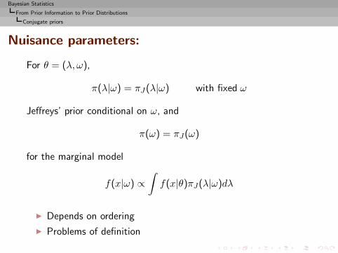
Nuisance parameters:
For θ = (λ, ω),
π(λ|ω) = πJ(λ|ω) with fixed ω
Jeffreys’ prior conditional on ω, and
π(ω) = πJ(ω)
for the marginal model
f(x|ω) ∝∫f(x|θ)πJ(λ|ω)dλ
◮ Depends on ordering
◮ Problems of definition
Bayesian Statistics
From Prior Information to Prior Distributions
Conjugate priors
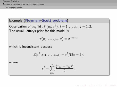
Example (Neyman–Scott problem)
Observation of xij iid N (µi, σ2), i = 1, . . . , n, j = 1, 2.
The usual Jeffreys prior for this model is
π(µ1, . . . , µn, σ) = σ−n−1
which is inconsistent because
E[σ2|x11, . . . , xn2] = s2/(2n − 2),
where
s2 =
n∑
i=1
(xi1 − xi2)2
2,
Bayesian Statistics
From Prior Information to Prior Distributions
Conjugate priors
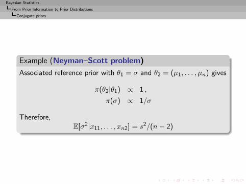
Example (Neyman–Scott problem)
Associated reference prior with θ1 = σ and θ2 = (µ1, . . . , µn) gives
π(θ2|θ1) ∝ 1 ,
π(σ) ∝ 1/σ
Therefore,E[σ2|x11, . . . , xn2] = s2/(n− 2)
Bayesian Statistics
From Prior Information to Prior Distributions
Conjugate priors
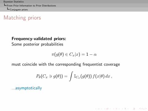
Matching priors
Frequency-validated priors:Some posterior probabilities
π(g(θ) ∈ Cx|x) = 1 − α
must coincide with the corresponding frequentist coverage
Pθ(Cx ∋ g(θ)) =
∫ICx(g(θ)) f(x|θ) dx ,
...asymptotically
Bayesian Statistics
From Prior Information to Prior Distributions
Conjugate priors
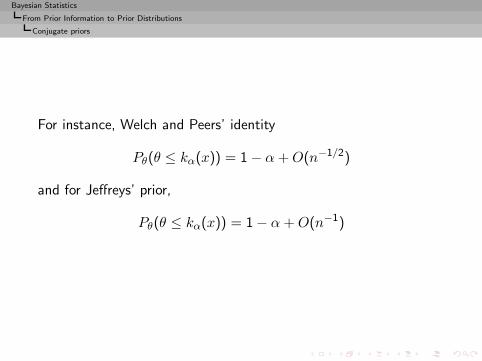
For instance, Welch and Peers’ identity
Pθ(θ ≤ kα(x)) = 1 − α+O(n−1/2)
and for Jeffreys’ prior,
Pθ(θ ≤ kα(x)) = 1 − α+O(n−1)
Bayesian Statistics
From Prior Information to Prior Distributions
Conjugate priors
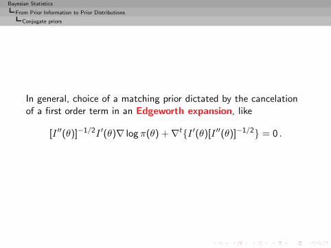
In general, choice of a matching prior dictated by the cancelationof a first order term in an Edgeworth expansion, like
[I ′′(θ)]−1/2I ′(θ)∇ log π(θ) + ∇t{I ′(θ)[I ′′(θ)]−1/2} = 0 .
Bayesian Statistics
From Prior Information to Prior Distributions
Conjugate priors
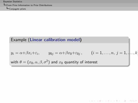
Example (Linear calibration model)
yi = α+βxi+εi, y0j = α+βx0+ε0j , (i = 1, . . . , n, j = 1, . . . , k)
with θ = (x0, α, β, σ2) and x0 quantity of interest
Bayesian Statistics
From Prior Information to Prior Distributions
Conjugate priors
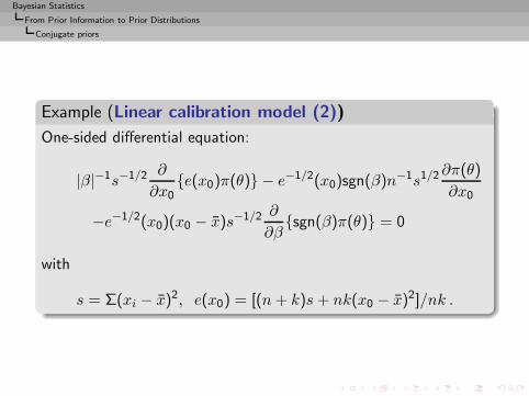
Example (Linear calibration model (2))
One-sided differential equation:
|β|−1s−1/2 ∂
∂x0{e(x0)π(θ)} − e−1/2(x0)sgn(β)n−1s1/2
∂π(θ)
∂x0
−e−1/2(x0)(x0 − x)s−1/2 ∂
∂β{sgn(β)π(θ)} = 0
with
s = Σ(xi − x)2, e(x0) = [(n+ k)s + nk(x0 − x)2]/nk .
Bayesian Statistics
From Prior Information to Prior Distributions
Conjugate priors
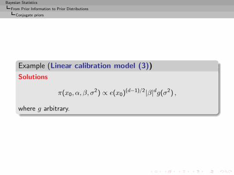
Example (Linear calibration model (3))
Solutions
π(x0, α, β, σ2) ∝ e(x0)
(d−1)/2|β|dg(σ2) ,
where g arbitrary.
Bayesian Statistics
From Prior Information to Prior Distributions
Conjugate priors
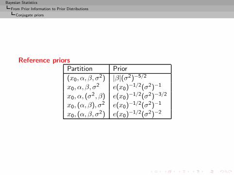
Reference priorsPartition Prior
(x0, α, β, σ2) |β|(σ2)−5/2
x0, α, β, σ2 e(x0)
−1/2(σ2)−1
x0, α, (σ2, β) e(x0)
−1/2(σ2)−3/2
x0, (α, β), σ2 e(x0)−1/2(σ2)−1
x0, (α, β, σ2) e(x0)
−1/2(σ2)−2

Bayesian Statistics
From Prior Information to Prior Distributions
Conjugate priors
Other approaches
◮ Rissanen’s transmission information theory and minimumlength priors
◮ Testing priors
◮ stochastic complexity
Bayesian Statistics
Bayesian Point Estimation
Bayesian Point Estimation
Introduction
Decision-Theoretic Foundations of Statistical Inference
From Prior Information to Prior Distributions
Bayesian Point EstimationBayesian inferenceBayesian Decision TheoryThe particular case of the normal modelDynamic models
Bayesian Calculations
Bayesian Statistics
Bayesian Point Estimation
Posterior distribution
π(θ|x) ∝ f(x|θ)π(θ)
◮ extensive summary of the information available on θ
◮ integrate simultaneously prior information and informationbrought by x
◮ unique motor of inference
Bayesian Statistics
Bayesian Point Estimation
Bayesian inference
MAP estimator
With no loss function, consider using the maximum a posteriori(MAP) estimator
arg maxθℓ(θ|x)π(θ)
Bayesian Statistics
Bayesian Point Estimation
Bayesian inference
Motivations
◮ Associated with 0 − 1 losses and Lp losses
◮ Penalized likelihood estimator
◮ Further appeal in restricted parameter spaces
Bayesian Statistics
Bayesian Point Estimation
Bayesian inference
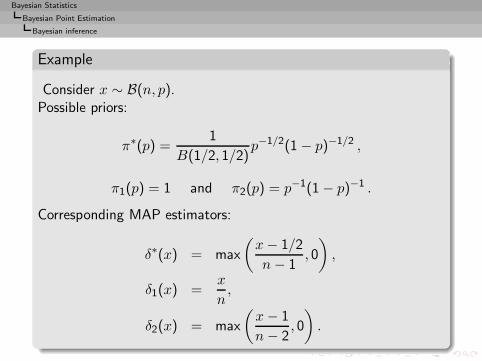
Example
Consider x ∼ B(n, p).Possible priors:
π∗(p) =1
B(1/2, 1/2)p−1/2(1 − p)−1/2 ,
π1(p) = 1 and π2(p) = p−1(1 − p)−1 .
Corresponding MAP estimators:
δ∗(x) = max
(x− 1/2
n− 1, 0
),
δ1(x) =x
n,
δ2(x) = max
(x− 1
n− 2, 0
).
Bayesian Statistics
Bayesian Point Estimation
Bayesian inference
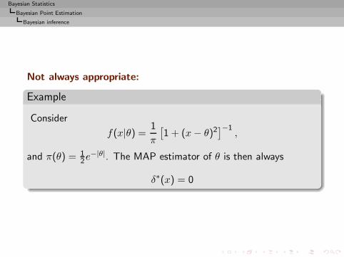
Not always appropriate:
Example
Consider
f(x|θ) =1
π
[1 + (x− θ)2
]−1,
and π(θ) = 12e
−|θ|. The MAP estimator of θ is then always
δ∗(x) = 0
Bayesian Statistics
Bayesian Point Estimation
Bayesian inference
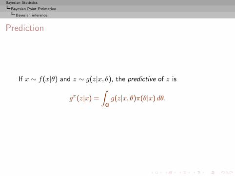
Prediction
If x ∼ f(x|θ) and z ∼ g(z|x, θ), the predictive of z is
gπ(z|x) =
∫
Θg(z|x, θ)π(θ|x) dθ.
Bayesian Statistics
Bayesian Point Estimation
Bayesian inference
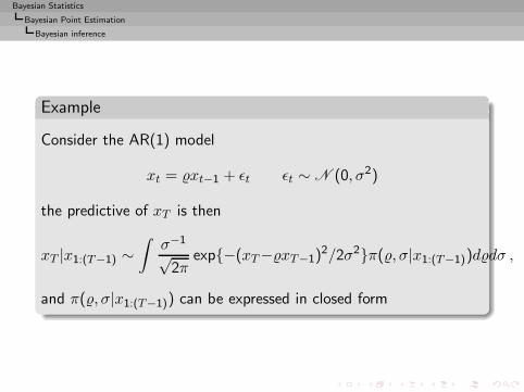
Example
Consider the AR(1) model
xt = xt−1 + ǫt ǫt ∼ N (0, σ2)
the predictive of xT is then
xT |x1:(T−1) ∼∫
σ−1
√2π
exp{−(xT−xT−1)2/2σ2}π(, σ|x1:(T−1))ddσ ,
and π(, σ|x1:(T−1)) can be expressed in closed form
Bayesian Statistics
Bayesian Point Estimation
Bayesian Decision Theory
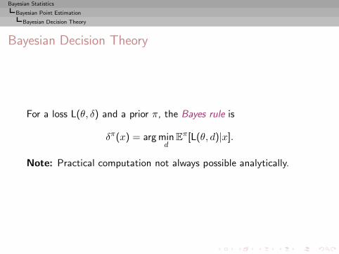
Bayesian Decision Theory
For a loss L(θ, δ) and a prior π, the Bayes rule is
δπ(x) = arg mind
Eπ[L(θ, d)|x].
Note: Practical computation not always possible analytically.
Bayesian Statistics
Bayesian Point Estimation
Bayesian Decision Theory
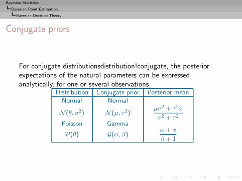
Conjugate priors
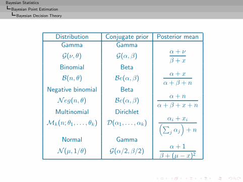
For conjugate distributionsdistribution!conjugate, the posteriorexpectations of the natural parameters can be expressedanalytically, for one or several observations.
Distribution Conjugate prior Posterior meanNormal Normal
N (θ, σ2) N (µ, τ2)µσ2 + τ2x
σ2 + τ2
Poisson Gamma
P(θ) G(α, β)α+ x
β + 1
Bayesian Statistics
Bayesian Point Estimation
Bayesian Decision Theory
Distribution Conjugate prior Posterior meanGamma Gamma
G(ν, θ) G(α, β)α+ ν
β + xBinomial Beta
B(n, θ) Be(α, β)α+ x
α+ β + nNegative binomial Beta
N eg(n, θ) Be(α, β)α+ n
α+ β + x+ nMultinomial Dirichlet
Mk(n; θ1, . . . , θk) D(α1, . . . , αk)αi + xi(∑j αj
)+ n
Normal Gamma
N (µ, 1/θ) G(α/2, β/2)α+ 1
β + (µ− x)2
Bayesian Statistics
Bayesian Point Estimation
Bayesian Decision Theory
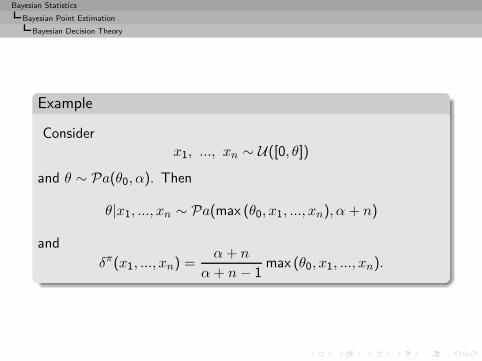
Example
Considerx1, ..., xn ∼ U([0, θ])
and θ ∼ Pa(θ0, α). Then
θ|x1, ..., xn ∼ Pa(max (θ0, x1, ..., xn), α + n)
and
δπ(x1, ..., xn) =α+ n
α+ n− 1max (θ0, x1, ..., xn).
Bayesian Statistics
Bayesian Point Estimation
Bayesian Decision Theory
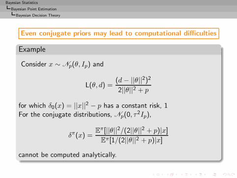
Even conjugate priors may lead to computational difficulties
Example
Consider x ∼ Np(θ, Ip) and
L(θ, d) =(d− ||θ||2)22||θ||2 + p
for which δ0(x) = ||x||2 − p has a constant risk, 1For the conjugate distributions, Np(0, τ
2Ip),
δπ(x) =Eπ[||θ||2/(2||θ||2 + p)|x]
Eπ[1/(2||θ||2 + p)|x]
cannot be computed analytically.
Bayesian Statistics
Bayesian Point Estimation
The particular case of the normal model
The normal model
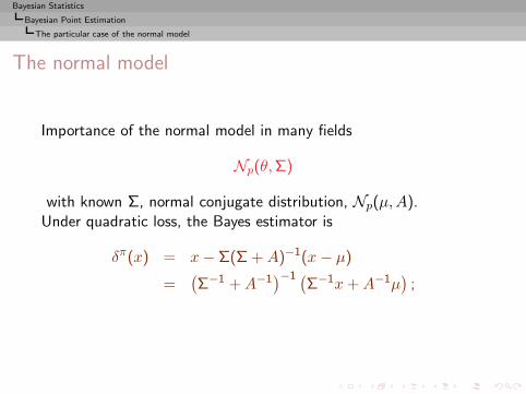
Importance of the normal model in many fields
Np(θ,Σ)
with known Σ, normal conjugate distribution, Np(µ,A).Under quadratic loss, the Bayes estimator is
δπ(x) = x− Σ(Σ +A)−1(x− µ)
=(Σ−1 +A−1
)−1 (Σ−1x+A−1µ
);
Bayesian Statistics
Bayesian Point Estimation
The particular case of the normal model
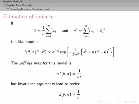
Estimation of varianceIf
x =1
n
n∑
i=1
xi and s2 =n∑
i=1
(xi − x)2
the likelihood is
ℓ(θ, σ | x, s2) ∝ σ−n exp
[− 1
2σ2
{s2 + n (x− θ)2
}]
The Jeffreys prior for this model is
π∗(θ, σ) =1
σ2
but invariance arguments lead to prefer
π(θ, σ) =1
σ
Bayesian Statistics
Bayesian Point Estimation
The particular case of the normal model
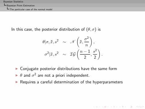
In this case, the posterior distribution of (θ, σ) is
θ|σ, x, s2 ∼ N
(x,σ2
n
),
σ2|x, s2 ∼ IG(n− 1
2,s2
2
).
◮ Conjugate posterior distributions have the same form
◮ θ and σ2 are not a priori independent.
◮ Requires a careful determination of the hyperparameters
Bayesian Statistics
Bayesian Point Estimation
The particular case of the normal model
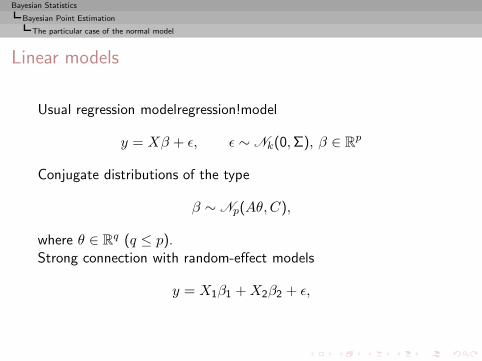
Linear models
Usual regression modelregression!model
y = Xβ + ǫ, ǫ ∼ Nk(0,Σ), β ∈ Rp
Conjugate distributions of the type
β ∼ Np(Aθ,C),
where θ ∈ Rq (q ≤ p).Strong connection with random-effect models
y = X1β1 +X2β2 + ǫ,
Bayesian Statistics
Bayesian Point Estimation
The particular case of the normal model
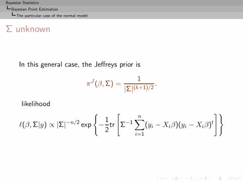
Σ unknown
In this general case, the Jeffreys prior is
πJ(β,Σ) =1
|Σ|(k+1)/2.
likelihood
ℓ(β,Σ|y) ∝ |Σ|−n/2 exp
{−1
2tr
[Σ−1
n∑
i=1
(yi −Xiβ)(yi −Xiβ)t
]}

Bayesian Statistics
Bayesian Point Estimation
The particular case of the normal model
◮ suggests (inverse) Wishart distribution on Σ
◮ posterior marginal distribution on β only defined for samplesize large enough
◮ no closed form expression for posterior marginal
Bayesian Statistics
Bayesian Point Estimation
The particular case of the normal model
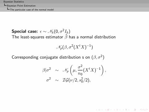
Special case: ǫ ∼ Nk(0, σ2Ik)
The least-squares estimator β has a normal distribution
Np(β, σ2(XtX)−1)
Corresponding conjugate distribution s on (β, σ2)
β|σ2 ∼ Np
(µ,σ2
n0(XtX)−1
),
σ2 ∼ IG(ν/2, s20/2),
Bayesian Statistics
Bayesian Point Estimation
The particular case of the normal model
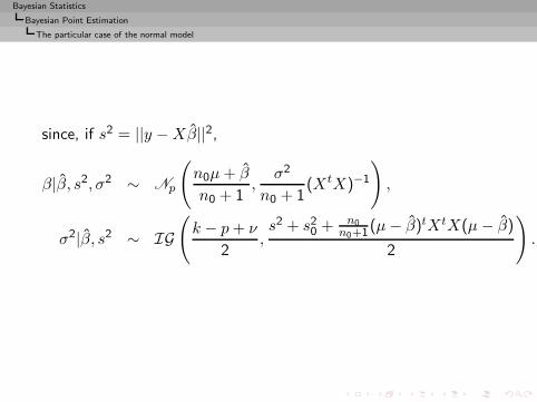
since, if s2 = ||y −Xβ||2,
β|β, s2, σ2 ∼ Np
(n0µ+ β
n0 + 1,
σ2
n0 + 1(XtX)−1
),
σ2|β, s2 ∼ IG(k − p+ ν
2,s2 + s20 + n0
n0+1(µ− β)tXtX(µ− β)
2
).
Bayesian Statistics
Bayesian Point Estimation
Dynamic models
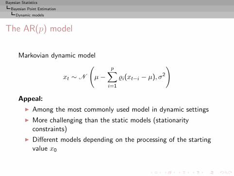
The AR(p) model
Markovian dynamic model
xt ∼ N
(µ−
p∑
i=1
i(xt−i − µ), σ2
)
Appeal:
◮ Among the most commonly used model in dynamic settings
◮ More challenging than the static models (stationarityconstraints)
◮ Different models depending on the processing of the startingvalue x0
Bayesian Statistics
Bayesian Point Estimation
Dynamic models
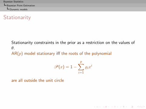
Stationarity
Stationarity constraints in the prior as a restriction on the values ofθ.AR(p) model stationary iff the roots of the polynomial
P(x) = 1 −p∑
i=1
ixi
are all outside the unit circle
Bayesian Statistics
Bayesian Point Estimation
Dynamic models
Closed form likelihood
Conditional on the negative time values
L(µ, 1, . . . , p, σ|x1:T , x0:(−p+1)) =
σ−TT∏
t=1
exp
−(xt − µ+
p∑
i=1
i(xt−i − µ)
)2 /2σ2
,
Natural conjugate prior for θ = (µ, 1, . . . , p, σ2) :
a normal distributiondistribution!normal on (µ, 1, . . . , ρp) and aninverse gamma distributiondistribution!inverse gamma on σ2.
Bayesian Statistics
Bayesian Point Estimation
Dynamic models
Stationarity & priors
Under stationarity constraint, complex parameter spaceThe Durbin–Levinson recursion proposes a reparametrization fromthe parameters i to the partial autocorrelations
ψi ∈ [−1, 1]
which allow for a uniform prior.

Bayesian Statistics
Bayesian Point Estimation
Dynamic models
Transform:
0. Define ϕii = ψi and ϕij = ϕ(i−1)j − ψiϕ(i−1)(i−j), for i > 1
and j = 1, · · · , i− 1 .
1. Take i = ϕpi for i = 1, · · · , p.
Different approach via the real+complex roots of the polynomialP, whose inverses are also within the unit circle.
Bayesian Statistics
Bayesian Point Estimation
Dynamic models
Stationarity & priors (contd.)
Jeffreys’ prior associated with the stationaryrepresentationrepresentation!stationary is
πJ1 (µ, σ2, ) ∝ 1
σ2
1√1 − 2
.
Within the non-stationary region || > 1, the Jeffreys prior is
πJ2 (µ, σ2, ) ∝ 1
σ2
1√|1 − 2|
√∣∣∣∣1 − 1 − 2T
T (1 − 2)
∣∣∣∣ .
The dominant part of the prior is the non-stationary region!
Bayesian Statistics
Bayesian Point Estimation
Dynamic models
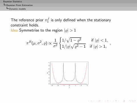
The reference prior πJ1 is only defined when the stationaryconstraint holds.Idea Symmetrise to the region || > 1
πB(µ, σ2, ) ∝ 1
σ2
{1/√
1 − 2 if || < 1,
1/||√2 − 1 if || > 1,
,
−3 −2 −1 0 1 2 3
01
23
45
67
x
pi
Bayesian Statistics
Bayesian Point Estimation
Dynamic models
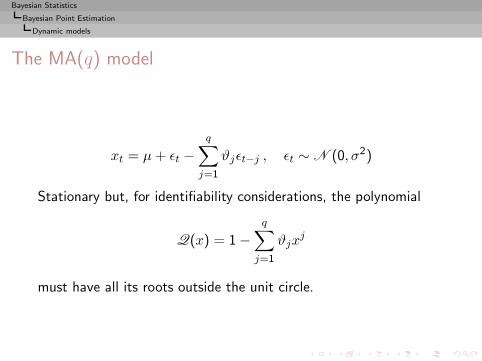
The MA(q) model
xt = µ+ ǫt −q∑
j=1
ϑjǫt−j , ǫt ∼ N (0, σ2)
Stationary but, for identifiability considerations, the polynomial
Q(x) = 1 −q∑
j=1
ϑjxj
must have all its roots outside the unit circle.
Bayesian Statistics
Bayesian Point Estimation
Dynamic models
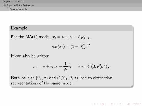
Example
For the MA(1) model, xt = µ+ ǫt − ϑ1ǫt−1,
var(xt) = (1 + ϑ21)σ
2
It can also be written
xt = µ+ ǫt−1 −1
ϑ1ǫt, ǫ ∼ N (0, ϑ2
1σ2) ,
Both couples (ϑ1, σ) and (1/ϑ1, ϑ1σ) lead to alternativerepresentations of the same model.
Bayesian Statistics
Bayesian Point Estimation
Dynamic models
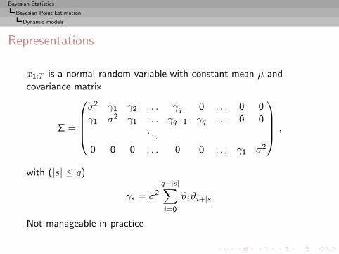
Representations
x1:T is a normal random variable with constant mean µ andcovariance matrix
Σ =
σ2 γ1 γ2 . . . γq 0 . . . 0 0γ1 σ2 γ1 . . . γq−1 γq . . . 0 0
. . .
0 0 0 . . . 0 0 . . . γ1 σ2
,
with (|s| ≤ q)
γs = σ2
q−|s|∑
i=0
ϑiϑi+|s|
Not manageable in practice
Bayesian Statistics
Bayesian Point Estimation
Dynamic models
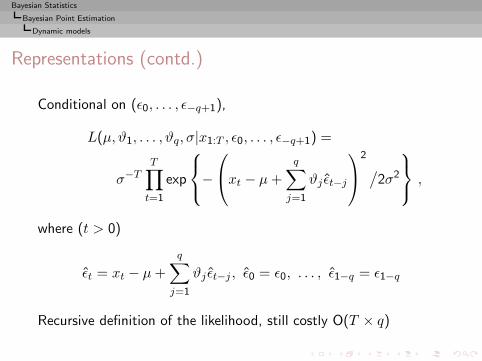
Representations (contd.)
Conditional on (ǫ0, . . . , ǫ−q+1),
L(µ, ϑ1, . . . , ϑq, σ|x1:T , ǫ0, . . . , ǫ−q+1) =
σ−TT∏
t=1
exp
−
xt − µ+
q∑
j=1
ϑj ǫt−j
2
/2σ2
,
where (t > 0)
ǫt = xt − µ+
q∑
j=1
ϑj ǫt−j , ǫ0 = ǫ0, . . . , ǫ1−q = ǫ1−q
Recursive definition of the likelihood, still costly O(T × q)
Bayesian Statistics
Bayesian Point Estimation
Dynamic models
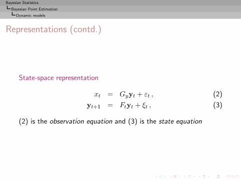
Representations (contd.)
State-space representation
xt = Gyyt + εt , (2)
yt+1 = Ftyt + ξt , (3)
(2) is the observation equation and (3) is the state equation
Bayesian Statistics
Bayesian Point Estimation
Dynamic models
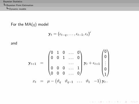
For the MA(q) model
yt = (ǫt−q, . . . , ǫt−1, ǫt)′
and
yt+1 =
0 1 0 . . . 00 0 1 . . . 0
. . .0 0 0 . . . 10 0 0 . . . 0
yt + ǫt+1
00...01
xt = µ−(ϑq ϑq−1 . . . ϑ1 −1
)yt .
Bayesian Statistics
Bayesian Point Estimation
Dynamic models
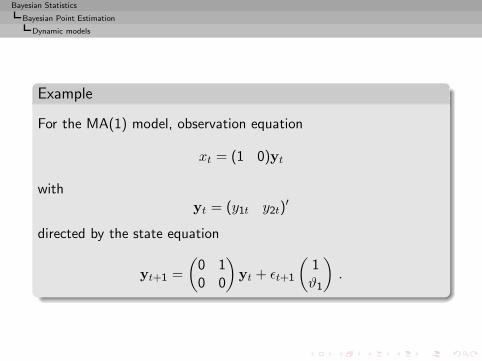
Example
For the MA(1) model, observation equation
xt = (1 0)yt
withyt = (y1t y2t)
′
directed by the state equation
yt+1 =
(0 10 0
)yt + ǫt+1
(1ϑ1
).
Bayesian Statistics
Bayesian Point Estimation
Dynamic models
Identifiability
Identifiability condition on Q(x): the ϑj’s vary in a complex space.New reparametrization: the ψi’s are the inverse partialauto-correlations
Bayesian Statistics
Bayesian Calculations
Bayesian Calculations
Introduction
Decision-Theoretic Foundations of Statistical Inference
From Prior Information to Prior Distributions
Bayesian Point Estimation
Bayesian CalculationsImplementation difficultiesClassical approximation methodsMarkov chain Monte Carlo methods
Tests and model choice
Bayesian Statistics
Bayesian Calculations
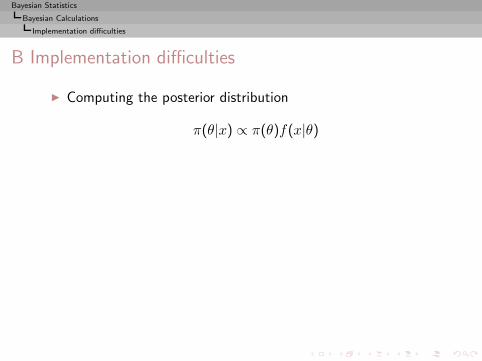
Implementation difficulties
B Implementation difficulties
◮ Computing the posterior distribution
π(θ|x) ∝ π(θ)f(x|θ)
Bayesian Statistics
Bayesian Calculations
Implementation difficulties
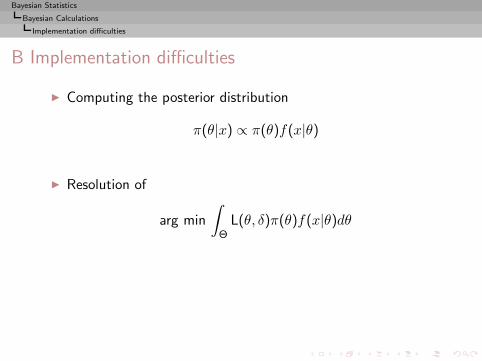
B Implementation difficulties
◮ Computing the posterior distribution
π(θ|x) ∝ π(θ)f(x|θ)
◮ Resolution of
arg min
∫
ΘL(θ, δ)π(θ)f(x|θ)dθ
Bayesian Statistics
Bayesian Calculations
Implementation difficulties
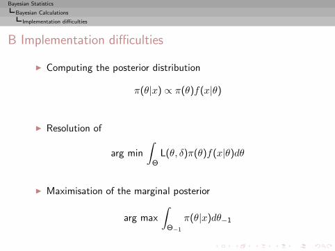
B Implementation difficulties
◮ Computing the posterior distribution
π(θ|x) ∝ π(θ)f(x|θ)
◮ Resolution of
arg min
∫
ΘL(θ, δ)π(θ)f(x|θ)dθ
◮ Maximisation of the marginal posterior
arg max
∫
Θ−1
π(θ|x)dθ−1
Bayesian Statistics
Bayesian Calculations
Implementation difficulties
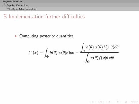
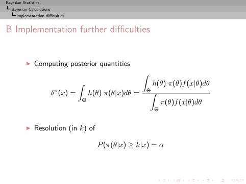
B Implementation further difficulties
◮ Computing posterior quantities
δπ(x) =
∫
Θh(θ) π(θ|x)dθ =
∫
Θh(θ) π(θ)f(x|θ)dθ∫
Θπ(θ)f(x|θ)dθ
Bayesian Statistics
Bayesian Calculations
Implementation difficulties
B Implementation further difficulties
◮ Computing posterior quantities
δπ(x) =
∫
Θh(θ) π(θ|x)dθ =
∫
Θh(θ) π(θ)f(x|θ)dθ∫
Θπ(θ)f(x|θ)dθ
◮ Resolution (in k) of
P (π(θ|x) ≥ k|x) = α
Bayesian Statistics
Bayesian Calculations
Implementation difficulties
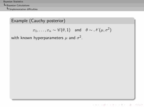
Example (Cauchy posterior)
x1, . . . , xn ∼ C (θ, 1) and θ ∼ N (µ, σ2)
with known hyperparameters µ and σ2.
Bayesian Statistics
Bayesian Calculations
Implementation difficulties
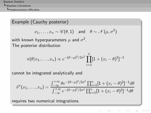
Example (Cauchy posterior)
x1, . . . , xn ∼ C (θ, 1) and θ ∼ N (µ, σ2)
with known hyperparameters µ and σ2.The posterior distribution
π(θ|x1, . . . , xn) ∝ e−(θ−µ)2/2σ2n∏
i=1
[1 + (xi − θ)2]−1
cannot be integrated analytically and
δπ(x1, . . . , xn) =
∫ +∞−∞ θe−(θ−µ)2/2σ2 ∏n
i=1[1 + (xi − θ)2]−1dθ∫ +∞−∞ e−(θ−µ)2/2σ2 ∏n
i=1[1 + (xi − θ)2]−1dθ
requires two numerical integrations.
Bayesian Statistics
Bayesian Calculations
Implementation difficulties
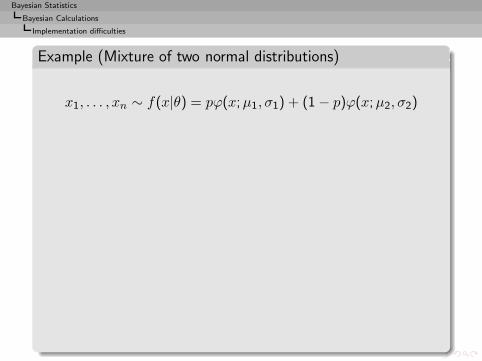
Example (Mixture of two normal distributions)
x1, . . . , xn ∼ f(x|θ) = pϕ(x;µ1, σ1) + (1 − p)ϕ(x;µ2, σ2)
Bayesian Statistics
Bayesian Calculations
Implementation difficulties
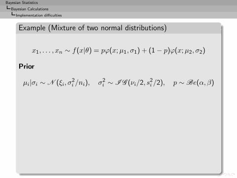
Example (Mixture of two normal distributions)
x1, . . . , xn ∼ f(x|θ) = pϕ(x;µ1, σ1) + (1 − p)ϕ(x;µ2, σ2)
Prior
µi|σi ∼ N (ξi, σ2i /ni), σ2
i ∼ I G (νi/2, s2i /2), p ∼ Be(α, β)
Bayesian Statistics
Bayesian Calculations
Implementation difficulties
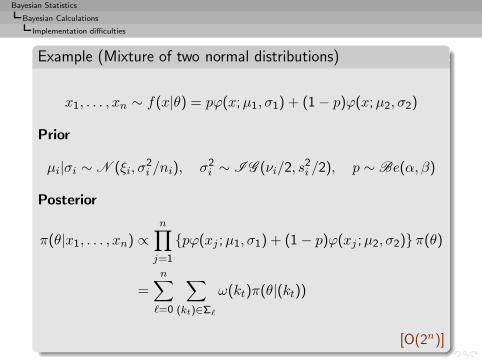
Example (Mixture of two normal distributions)
x1, . . . , xn ∼ f(x|θ) = pϕ(x;µ1, σ1) + (1 − p)ϕ(x;µ2, σ2)
Prior
µi|σi ∼ N (ξi, σ2i /ni), σ2
i ∼ I G (νi/2, s2i /2), p ∼ Be(α, β)
Posterior
π(θ|x1, . . . , xn) ∝n∏
j=1
{pϕ(xj ;µ1, σ1) + (1 − p)ϕ(xj ;µ2, σ2)}π(θ)
=
n∑
ℓ=0
∑
(kt)∈Σℓ
ω(kt)π(θ|(kt))
[O(2n)]
Bayesian Statistics
Bayesian Calculations
Implementation difficulties
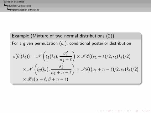
Example (Mixture of two normal distributions (2))
For a given permutation (kt), conditional posterior distribution
π(θ|(kt)) = N
(ξ1(kt),
σ21
n1 + ℓ
)× I G ((ν1 + ℓ)/2, s1(kt)/2)
× N
(ξ2(kt),
σ22
n2 + n− ℓ
)× I G ((ν2 + n− ℓ)/2, s2(kt)/2)
× Be(α+ ℓ, β + n− ℓ)
Bayesian Statistics
Bayesian Calculations
Implementation difficulties
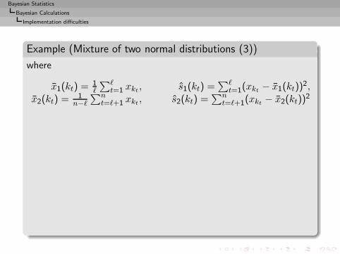
Example (Mixture of two normal distributions (3))
where
x1(kt) = 1ℓ
∑ℓt=1 xkt , s1(kt) =
∑ℓt=1(xkt − x1(kt))
2,x2(kt) = 1
n−ℓ∑n
t=ℓ+1 xkt , s2(kt) =∑n
t=ℓ+1(xkt − x2(kt))2
Bayesian Statistics
Bayesian Calculations
Implementation difficulties
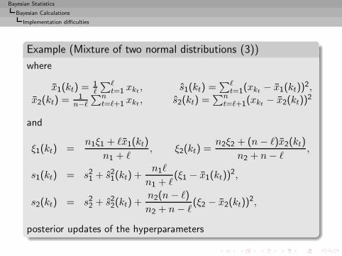
Example (Mixture of two normal distributions (3))
where
x1(kt) = 1ℓ
∑ℓt=1 xkt , s1(kt) =
∑ℓt=1(xkt − x1(kt))
2,x2(kt) = 1
n−ℓ∑n
t=ℓ+1 xkt , s2(kt) =∑n
t=ℓ+1(xkt − x2(kt))2
and
ξ1(kt) =n1ξ1 + ℓx1(kt)
n1 + ℓ, ξ2(kt) =
n2ξ2 + (n− ℓ)x2(kt)
n2 + n− ℓ,
s1(kt) = s21 + s21(kt) +n1ℓ
n1 + ℓ(ξ1 − x1(kt))
2,
s2(kt) = s22 + s22(kt) +n2(n − ℓ)
n2 + n− ℓ(ξ2 − x2(kt))
2,
posterior updates of the hyperparameters
Bayesian Statistics
Bayesian Calculations
Implementation difficulties
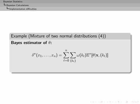
Example (Mixture of two normal distributions (4))
Bayes estimator of θ:
δπ(x1, . . . , xn) =
n∑
ℓ=0
∑
(kt)
ω(kt)Eπ[θ|x, (kt)]
Bayesian Statistics
Bayesian Calculations
Implementation difficulties
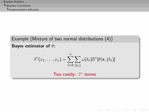
Example (Mixture of two normal distributions (4))
Bayes estimator of θ:
δπ(x1, . . . , xn) =
n∑
ℓ=0
∑
(kt)
ω(kt)Eπ[θ|x, (kt)]
Too costly: 2n terms

Bayesian Statistics
Bayesian Calculations
Classical approximation methods
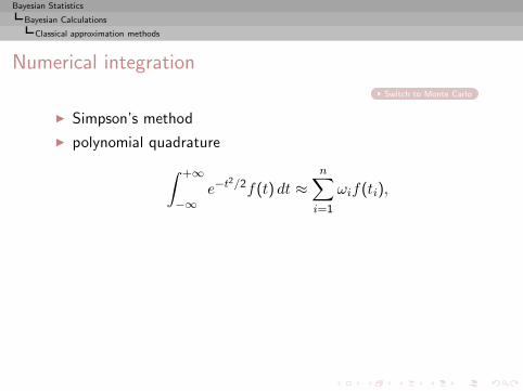
Numerical integration
Switch to Monte Carlo
◮ Simpson’s method
Bayesian Statistics
Bayesian Calculations
Classical approximation methods
Numerical integration
Switch to Monte Carlo
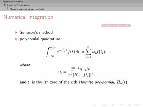
◮ Simpson’s method
◮ polynomial quadrature
∫ +∞
−∞e−t
2/2f(t) dt ≈n∑
i=1
ωif(ti),
Bayesian Statistics
Bayesian Calculations
Classical approximation methods
Numerical integration
Switch to Monte Carlo
◮ Simpson’s method
◮ polynomial quadrature
∫ +∞
−∞e−t
2/2f(t) dt ≈n∑
i=1
ωif(ti),
where
ωi =2n−1n!
√n
n2[Hn−1(ti)]2
and ti is the ith zero of the nth Hermite polynomial, Hn(t).
Bayesian Statistics
Bayesian Calculations
Classical approximation methods
Numerical integration
Switch to Monte Carlo
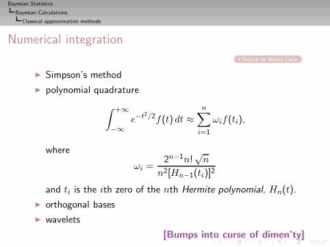
◮ Simpson’s method
◮ polynomial quadrature
∫ +∞
−∞e−t
2/2f(t) dt ≈n∑
i=1
ωif(ti),
where
ωi =2n−1n!
√n
n2[Hn−1(ti)]2
and ti is the ith zero of the nth Hermite polynomial, Hn(t).
◮ orthogonal bases
◮ wavelets
[Bumps into curse of dimen’ty]
Bayesian Statistics
Bayesian Calculations
Classical approximation methods
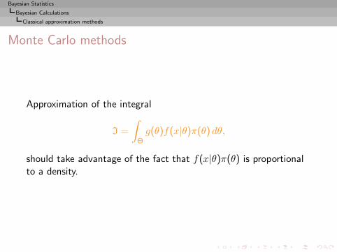
Monte Carlo methods
Approximation of the integral
I =
∫
Θg(θ)f(x|θ)π(θ) dθ,
should take advantage of the fact that f(x|θ)π(θ) is proportionalto a density.
Bayesian Statistics
Bayesian Calculations
Classical approximation methods
MC Principle
If the θi’s are generated from π(θ), the average
1
m
m∑
i=1
g(θi)f(x|θi)
converges (almost surely) to I
Bayesian Statistics
Bayesian Calculations
Classical approximation methods
MC Principle
If the θi’s are generated from π(θ), the average
1
m
m∑
i=1
g(θi)f(x|θi)
converges (almost surely) to I
Confidence regions can be derived from a normal approximationand the magnitude of the error remains of order
1/√m,
whatever the dimension of the problem.[Commercial!!]
Bayesian Statistics
Bayesian Calculations
Classical approximation methods
Importance function
No need to simulate from π(·|x) or from π
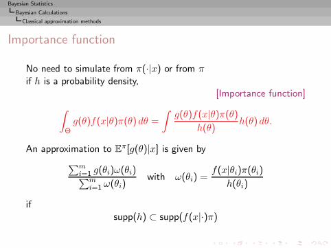
Bayesian Statistics
Bayesian Calculations
Classical approximation methods
Importance function
No need to simulate from π(·|x) or from πif h is a probability density,
[Importance function]
∫
Θg(θ)f(x|θ)π(θ) dθ =
∫g(θ)f(x|θ)π(θ)
h(θ)h(θ) dθ.
An approximation to Eπ[g(θ)|x] is given by
∑mi=1 g(θi)ω(θi)∑m
i=1 ω(θi)with ω(θi) =
f(x|θi)π(θi)
h(θi)
ifsupp(h) ⊂ supp(f(x|·)π)

Bayesian Statistics
Bayesian Calculations
Classical approximation methods
Requirements
◮ Simulation from h must be easy
Bayesian Statistics
Bayesian Calculations
Classical approximation methods
Requirements
◮ Simulation from h must be easy
◮ h(θ) must be close enough to g(θ)π(θ|x)
Bayesian Statistics
Bayesian Calculations
Classical approximation methods
Requirements
◮ Simulation from h must be easy
◮ h(θ) must be close enough to g(θ)π(θ|x)◮ the variance of the importance sampling estimator must be
finite
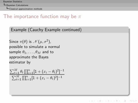
Bayesian Statistics
Bayesian Calculations
Classical approximation methods
The importance function may be π
Example (Cauchy Example continued)
Since π(θ) is N (µ, σ2),possible to simulate a normalsample θ1, . . . , θM and toapproximate the Bayesestimator by
∑Mt=1 θt
∏ni=1[1 + (xi − θt)
2]−1
∑Mt=1
∏ni=1[1 + (xi − θt)2]−1
mu
varia
tion
0 2 4 6 8 10
-0.5
0.0
0.5
90% variation
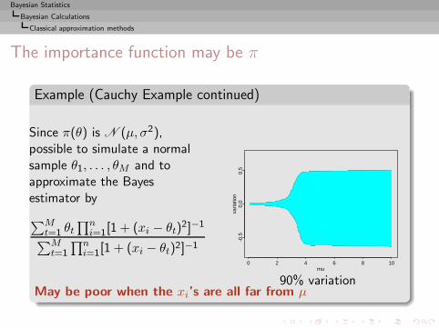
Bayesian Statistics
Bayesian Calculations
Classical approximation methods
The importance function may be π
Example (Cauchy Example continued)
Since π(θ) is N (µ, σ2),possible to simulate a normalsample θ1, . . . , θM and toapproximate the Bayesestimator by
∑Mt=1 θt
∏ni=1[1 + (xi − θt)
2]−1
∑Mt=1
∏ni=1[1 + (xi − θt)2]−1
mu
varia
tion
0 2 4 6 8 10
-0.5
0.0
0.5
90% variationMay be poor when the xi’s are all far from µ
Bayesian Statistics
Bayesian Calculations
Classical approximation methods
Defensive sampling
Use a mix of prior and posterior
h(θ) = ρπ(θ) + (1 − ρ)π(θ|x) ρ≪ 1
[Newton & Raftery, 1994]

Bayesian Statistics
Bayesian Calculations
Classical approximation methods
Defensive sampling
Use a mix of prior and posterior
h(θ) = ρπ(θ) + (1 − ρ)π(θ|x) ρ≪ 1
[Newton & Raftery, 1994]Requires proper knowledge of normalising constants
[Bummer!]
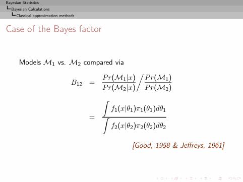
Bayesian Statistics
Bayesian Calculations
Classical approximation methods
Case of the Bayes factor
Models M1 vs. M2 compared via
B12 =Pr(M1|x)Pr(M2|x)
/Pr(M1)
Pr(M2)
=
∫f1(x|θ1)π1(θ1)dθ1
∫f2(x|θ2)π2(θ2)dθ2
[Good, 1958 & Jeffreys, 1961]
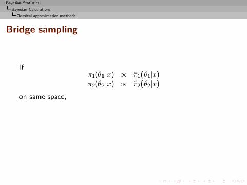
Bayesian Statistics
Bayesian Calculations
Classical approximation methods
Bridge sampling
Ifπ1(θ1|x) ∝ π1(θ1|x)π2(θ2|x) ∝ π2(θ2|x)
on same space,
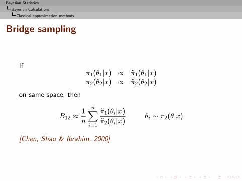
Bayesian Statistics
Bayesian Calculations
Classical approximation methods
Bridge sampling
Ifπ1(θ1|x) ∝ π1(θ1|x)π2(θ2|x) ∝ π2(θ2|x)
on same space, then
B12 ≈ 1
n
n∑
i=1
π1(θi|x)π2(θi|x)
θi ∼ π2(θ|x)
[Chen, Shao & Ibrahim, 2000]
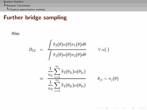
Bayesian Statistics
Bayesian Calculations
Classical approximation methods
Further bridge sampling
Also
B12 =
∫π2(θ)α(θ)π1(θ)dθ
∫π1(θ)α(θ)π2(θ)dθ
∀ α(·)
≈
1
n1
n1∑
i=1
π2(θ1i)α(θ1i)
1
n2
n2∑
i=1
π1(θ2i)α(θ2i)
θji ∼ πj(θ)
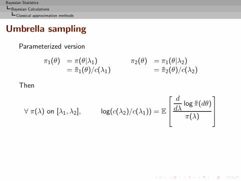
Bayesian Statistics
Bayesian Calculations
Classical approximation methods
Umbrella sampling
Parameterized version
π1(θ) = π(θ|λ1) π2(θ) = π1(θ|λ2)= π1(θ)/c(λ1) = π2(θ)/c(λ2)
Then
∀ π(λ) on [λ1, λ2], log(c(λ2)/c(λ1)) = E
d
dλlog π(dθ)
π(λ)
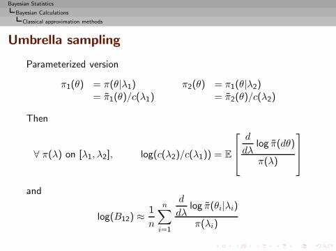
Bayesian Statistics
Bayesian Calculations
Classical approximation methods
Umbrella sampling
Parameterized version
π1(θ) = π(θ|λ1) π2(θ) = π1(θ|λ2)= π1(θ)/c(λ1) = π2(θ)/c(λ2)
Then
∀ π(λ) on [λ1, λ2], log(c(λ2)/c(λ1)) = E
d
dλlog π(dθ)
π(λ)
and
log(B12) ≈1
n
n∑
i=1
d
dλlog π(θi|λi)π(λi)
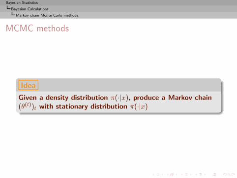
Bayesian Statistics
Bayesian Calculations
Markov chain Monte Carlo methods
MCMC methods
Idea
Given a density distribution π(·|x), produce a Markov chain(θ(t))t with stationary distribution π(·|x)

Bayesian Statistics
Bayesian Calculations
Markov chain Monte Carlo methods
Formal Warranty
Convergence
if the Markov chains produced by MCMC algorithms areirreducible, these chains are both positive recurrent with stationarydistribution π(θ|x) and ergodic.
Bayesian Statistics
Bayesian Calculations
Markov chain Monte Carlo methods
Formal Warranty
Convergence
if the Markov chains produced by MCMC algorithms areirreducible, these chains are both positive recurrent with stationarydistribution π(θ|x) and ergodic.
Translation:For k large enough, θ(k) is approximately distributed from π(θ|x),no matter what the starting value θ(0) is.

Bayesian Statistics
Bayesian Calculations
Markov chain Monte Carlo methods
Practical use
◮ Produce an i.i.d. sample θ1, . . . , θm from π(θ|x), taking thecurrent θ(k) as the new starting value
Bayesian Statistics
Bayesian Calculations
Markov chain Monte Carlo methods
Practical use
◮ Produce an i.i.d. sample θ1, . . . , θm from π(θ|x), taking thecurrent θ(k) as the new starting value
◮ Approximate Eπ[g(θ)|x] by Ergodic Theorem as
1
K
K∑
k=1
g(θ(k))
Bayesian Statistics
Bayesian Calculations
Markov chain Monte Carlo methods
Practical use
◮ Produce an i.i.d. sample θ1, . . . , θm from π(θ|x), taking thecurrent θ(k) as the new starting value
◮ Approximate Eπ[g(θ)|x] by Ergodic Theorem as
1
K
K∑
k=1
g(θ(k))
◮ Achieve quasi-independence by batch sampling
◮ Construct approximate posterior confidence regions
Cπx ≃ [θ(αT/2), θ(T−αT/2)]
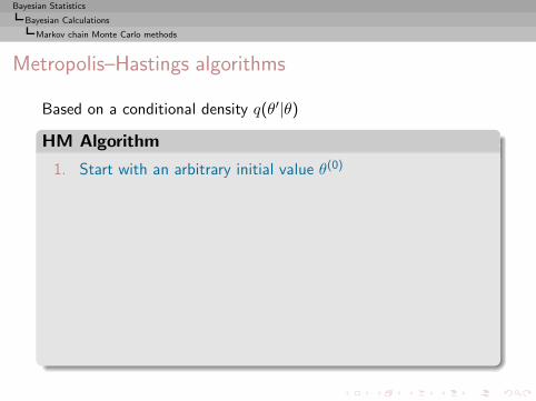
Bayesian Statistics
Bayesian Calculations
Markov chain Monte Carlo methods
Metropolis–Hastings algorithms
Based on a conditional density q(θ′|θ)
HM Algorithm
1. Start with an arbitrary initial value θ(0)
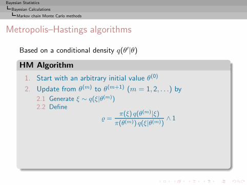
Bayesian Statistics
Bayesian Calculations
Markov chain Monte Carlo methods
Metropolis–Hastings algorithms
Based on a conditional density q(θ′|θ)
HM Algorithm
1. Start with an arbitrary initial value θ(0)
2. Update from θ(m) to θ(m+1) (m = 1, 2, . . .) by
2.1 Generate ξ ∼ q(ξ|θ(m))2.2 Define
=π(ξ) q(θ(m)|ξ)
π(θ(m)) q(ξ|θ(m))∧ 1
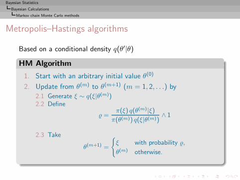
2.3 Take
θ(m+1) =
{ξ with probability ,
θ(m) otherwise.
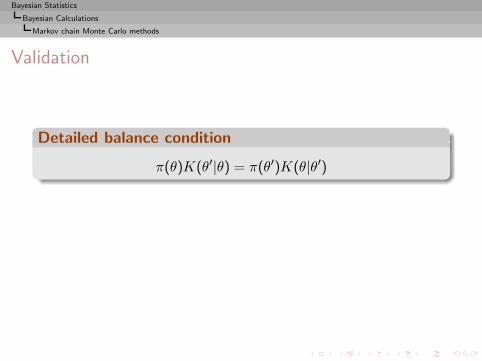
Bayesian Statistics
Bayesian Calculations
Markov chain Monte Carlo methods
Validation
Detailed balance condition
π(θ)K(θ′|θ) = π(θ′)K(θ|θ′)
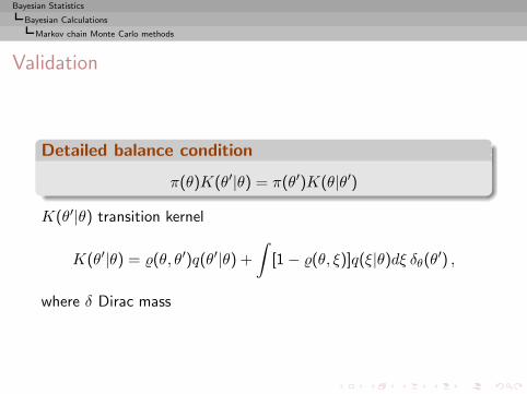
Bayesian Statistics
Bayesian Calculations
Markov chain Monte Carlo methods
Validation
Detailed balance condition
π(θ)K(θ′|θ) = π(θ′)K(θ|θ′)
K(θ′|θ) transition kernel
K(θ′|θ) = (θ, θ′)q(θ′|θ) +
∫[1 − (θ, ξ)]q(ξ|θ)dξ δθ(θ′) ,
where δ Dirac mass
Bayesian Statistics
Bayesian Calculations
Markov chain Monte Carlo methods
Random walk Metropolis–Hastings
Takeq(θ′|θ) = f(||θ′ − θ||)
Bayesian Statistics
Bayesian Calculations
Markov chain Monte Carlo methods
Random walk Metropolis–Hastings
Takeq(θ′|θ) = f(||θ′ − θ||)
Corresponding Metropolis–Hastings acceptance ratio
=π(ξ)
π(θ(m))∧ 1.

Bayesian Statistics
Bayesian Calculations
Markov chain Monte Carlo methods
Example (Repulsive normal)
For θ, x ∈ R2,
π(θ|x) ∝ exp{−||θ − x||2/2}p∏
i=1
exp
{ −1
||θ − µi||2},
where the µi’s are givenrepulsive points

Bayesian Statistics
Bayesian Calculations
Markov chain Monte Carlo methods
Example (Repulsive normal)
For θ, x ∈ R2,
π(θ|x) ∝ exp{−||θ − x||2/2}p∏
i=1
exp
{ −1
||θ − µi||2},
where the µi’s are givenrepulsive points
−4 −2 0 2 4
−4
−2
02
4x
y
Path of the Markov chain (5000iterations).

Bayesian Statistics
Bayesian Calculations
Markov chain Monte Carlo methods
Pros & Cons
◮ Widely applicable
◮ limited tune-up requirements (scale calibrated thruacceptance)
◮ never uniformely ergodic
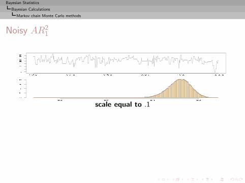
Bayesian Statistics
Bayesian Calculations
Markov chain Monte Carlo methods
Noisy AR21
scale equal to .1
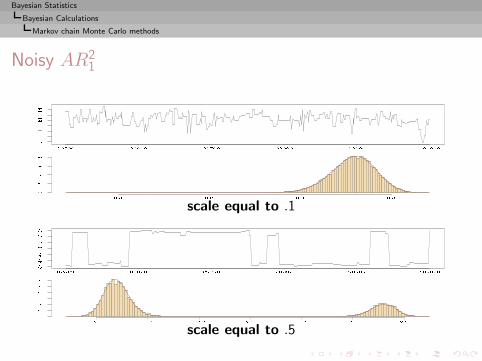
Bayesian Statistics
Bayesian Calculations
Markov chain Monte Carlo methods
Noisy AR21
scale equal to .1
scale equal to .5

Bayesian Statistics
Bayesian Calculations
Markov chain Monte Carlo methods
Independent proposals
Takeq(θ′|θ) = h(θ′) .

Bayesian Statistics
Bayesian Calculations
Markov chain Monte Carlo methods
Independent proposals
Takeq(θ′|θ) = h(θ′) .
More limited applicability and closer connection with iid simulation

Bayesian Statistics
Bayesian Calculations
Markov chain Monte Carlo methods
Independent proposals
Takeq(θ′|θ) = h(θ′) .
More limited applicability and closer connection with iid simulation
Examples
◮ prior distribution
◮ likelihood
◮ saddlepoint approximation

Bayesian Statistics
Bayesian Calculations
Markov chain Monte Carlo methods
The Gibbs sampler
Take advantage of hierarchical structures
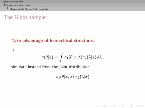
Bayesian Statistics
Bayesian Calculations
Markov chain Monte Carlo methods
The Gibbs sampler
Take advantage of hierarchical structures
If
π(θ|x) =
∫π1(θ|x, λ)π2(λ|x) dλ ,
simulate instead from the joint distribution
π1(θ|x, λ) π2(λ|x)
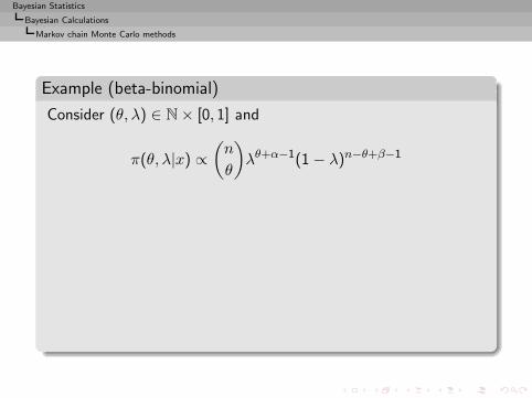
Bayesian Statistics
Bayesian Calculations
Markov chain Monte Carlo methods
Example (beta-binomial)
Consider (θ, λ) ∈ N × [0, 1] and
π(θ, λ|x) ∝(n
θ
)λθ+α−1(1 − λ)n−θ+β−1
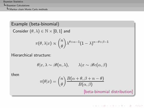
Bayesian Statistics
Bayesian Calculations
Markov chain Monte Carlo methods
Example (beta-binomial)
Consider (θ, λ) ∈ N × [0, 1] and
π(θ, λ|x) ∝(n
θ
)λθ+α−1(1 − λ)n−θ+β−1
Hierarchical structure:
θ|x, λ ∼ B(n, λ), λ|x ∼ Be(α, β)
then
π(θ|x) =
(n
θ
)B(α+ θ, β + n− θ)
B(α, β)
[beta-binomial distribution]

Bayesian Statistics
Bayesian Calculations
Markov chain Monte Carlo methods
Example (beta-binomial (2))
Difficult to work with this marginalFor instance, computation of E[θ/(θ + 1)|x] ?
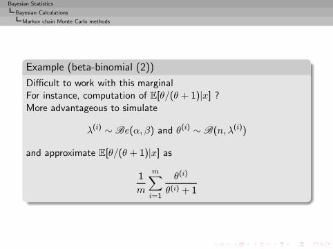
Bayesian Statistics
Bayesian Calculations
Markov chain Monte Carlo methods
Example (beta-binomial (2))
Difficult to work with this marginalFor instance, computation of E[θ/(θ + 1)|x] ?More advantageous to simulate
λ(i) ∼ Be(α, β) and θ(i) ∼ B(n, λ(i))
and approximate E[θ/(θ + 1)|x] as
1
m
m∑
i=1
θ(i)
θ(i) + 1

Bayesian Statistics
Bayesian Calculations
Markov chain Monte Carlo methods
Conditionals
Usually π2(λ|x) is not available/simulable
Bayesian Statistics
Bayesian Calculations
Markov chain Monte Carlo methods
Conditionals
Usually π2(λ|x) is not available/simulableMore often, both conditional posterior distributions,
π1(θ|x, λ) and π2(λ|x, θ)
can be simulated.
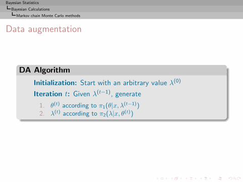
Bayesian Statistics
Bayesian Calculations
Markov chain Monte Carlo methods
Data augmentation
DA Algorithm
Initialization: Start with an arbitrary value λ(0)
Iteration t: Given λ(t−1), generate
1. θ(t) according to π1(θ|x, λ(t−1))2. λ(t) according to π2(λ|x, θ(t))
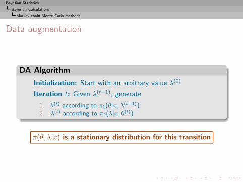
Bayesian Statistics
Bayesian Calculations
Markov chain Monte Carlo methods
Data augmentation
DA Algorithm
Initialization: Start with an arbitrary value λ(0)
Iteration t: Given λ(t−1), generate
1. θ(t) according to π1(θ|x, λ(t−1))2. λ(t) according to π2(λ|x, θ(t))
π(θ, λ|x) is a stationary distribution for this transition
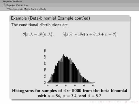
Bayesian Statistics
Bayesian Calculations
Markov chain Monte Carlo methods
Example (Beta-binomial Example cont’ed)
The conditional distributions are
θ|x, λ ∼ B(n, λ), λ|x, θ ∼ Be(α+ θ, β + n− θ)
0 10 20 30 40 50
0.0
0.01
0.02
0.03
0.04
0.05
0 10 20 30 40 50
0.0
0.01
0.02
0.03
0.04
0.05
0 10 20 30 40 50
0.0
0.01
0.02
0.03
0.04
0.05
Histograms for samples of size 5000 from the beta-binomialwith n = 54, α = 3.4, and β = 5.2
Bayesian Statistics
Bayesian Calculations
Markov chain Monte Carlo methods
Very simple example: Independent N(µ, σ2) obs’ions
When Y1, . . . , Yniid∼ N(y|µ, σ2) with both µ and σ unknown, the
posterior in (µ, σ2) is conjugate but non-standard
Bayesian Statistics
Bayesian Calculations
Markov chain Monte Carlo methods
Very simple example: Independent N(µ, σ2) obs’ions
When Y1, . . . , Yniid∼ N(y|µ, σ2) with both µ and σ unknown, the
posterior in (µ, σ2) is conjugate but non-standard
But...
µ|Y0:n, σ2 ∼ N
(µ∣∣∣ 1n∑n
i=1 Yi,σ2
n )
σ2|Y1:n, µ ∼ IG(σ2∣∣n2 − 1, 1
2
∑ni=1(Yi − µ)2
)
assuming constant (improper) priors on both µ and σ2
◮ Hence we may use the Gibbs sampler for simulating from theposterior of (µ, σ2)
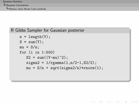
Bayesian Statistics
Bayesian Calculations
Markov chain Monte Carlo methods
R Gibbs Sampler for Gaussian posterior
n = length(Y);
S = sum(Y);
mu = S/n;
for (i in 1:500)
S2 = sum((Y-mu)^2);
sigma2 = 1/rgamma(1,n/2-1,S2/2);
mu = S/n + sqrt(sigma2/n)*rnorm(1);
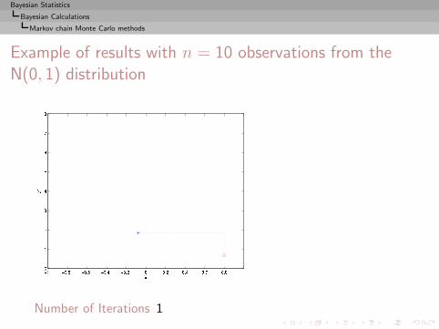
Bayesian Statistics
Bayesian Calculations
Markov chain Monte Carlo methods
Example of results with n = 10 observations from theN(0, 1) distribution
Number of Iterations 1
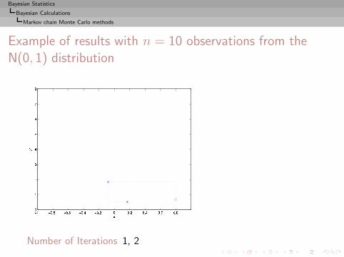
Bayesian Statistics
Bayesian Calculations
Markov chain Monte Carlo methods
Example of results with n = 10 observations from theN(0, 1) distribution
Number of Iterations 1, 2

Bayesian Statistics
Bayesian Calculations
Markov chain Monte Carlo methods
Example of results with n = 10 observations from theN(0, 1) distribution
Number of Iterations 1, 2, 3
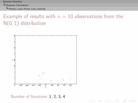
Bayesian Statistics
Bayesian Calculations
Markov chain Monte Carlo methods
Example of results with n = 10 observations from theN(0, 1) distribution
Number of Iterations 1, 2, 3, 4
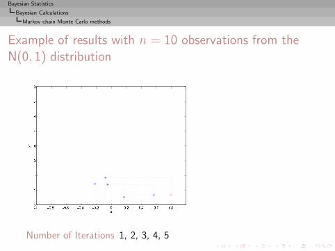
Bayesian Statistics
Bayesian Calculations
Markov chain Monte Carlo methods
Example of results with n = 10 observations from theN(0, 1) distribution
Number of Iterations 1, 2, 3, 4, 5
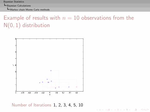
Bayesian Statistics
Bayesian Calculations
Markov chain Monte Carlo methods
Example of results with n = 10 observations from theN(0, 1) distribution
Number of Iterations 1, 2, 3, 4, 5, 10
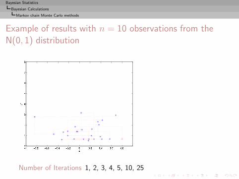
Bayesian Statistics
Bayesian Calculations
Markov chain Monte Carlo methods
Example of results with n = 10 observations from theN(0, 1) distribution
Number of Iterations 1, 2, 3, 4, 5, 10, 25
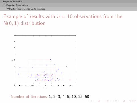
Bayesian Statistics
Bayesian Calculations
Markov chain Monte Carlo methods
Example of results with n = 10 observations from theN(0, 1) distribution
Number of Iterations 1, 2, 3, 4, 5, 10, 25, 50
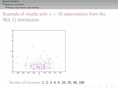
Bayesian Statistics
Bayesian Calculations
Markov chain Monte Carlo methods
Example of results with n = 10 observations from theN(0, 1) distribution
Number of Iterations 1, 2, 3, 4, 5, 10, 25, 50, 100
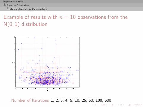
Bayesian Statistics
Bayesian Calculations
Markov chain Monte Carlo methods
Example of results with n = 10 observations from theN(0, 1) distribution
Number of Iterations 1, 2, 3, 4, 5, 10, 25, 50, 100, 500
Bayesian Statistics
Bayesian Calculations
Markov chain Monte Carlo methods
Rao–Blackwellization
Conditional structure of the sampling algorithm and the dualsample,
λ(1), . . . , λ(m),
should be exploited.
Bayesian Statistics
Bayesian Calculations
Markov chain Monte Carlo methods
Rao–Blackwellization
Conditional structure of the sampling algorithm and the dualsample,
λ(1), . . . , λ(m),
should be exploited.Eπ[g(θ)|x] can be approximated as
δ2 =1
m
m∑
i=1
Eπ[g(θ)|x, λ(m)],
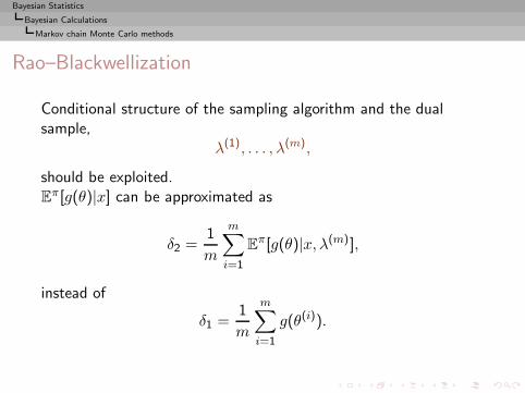
Bayesian Statistics
Bayesian Calculations
Markov chain Monte Carlo methods
Rao–Blackwellization
Conditional structure of the sampling algorithm and the dualsample,
λ(1), . . . , λ(m),
should be exploited.Eπ[g(θ)|x] can be approximated as
δ2 =1
m
m∑
i=1
Eπ[g(θ)|x, λ(m)],
instead of
δ1 =1
m
m∑
i=1
g(θ(i)).
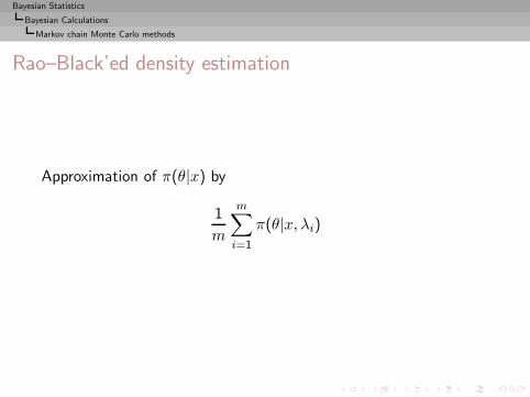
Bayesian Statistics
Bayesian Calculations
Markov chain Monte Carlo methods
Rao–Black’ed density estimation
Approximation of π(θ|x) by
1
m
m∑
i=1
π(θ|x, λi)
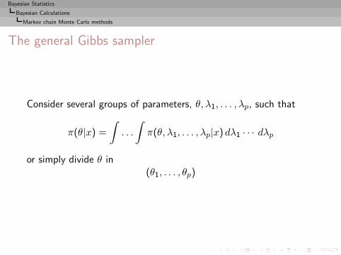
Bayesian Statistics
Bayesian Calculations
Markov chain Monte Carlo methods
The general Gibbs sampler
Consider several groups of parameters, θ, λ1, . . . , λp, such that
π(θ|x) =
∫. . .
∫π(θ, λ1, . . . , λp|x) dλ1 · · · dλp
or simply divide θ in(θ1, . . . , θp)
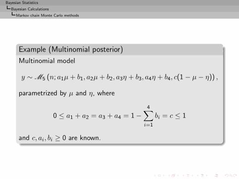
Bayesian Statistics
Bayesian Calculations
Markov chain Monte Carlo methods
Example (Multinomial posterior)
Multinomial model
y ∼ M5 (n; a1µ+ b1, a2µ+ b2, a3η + b3, a4η + b4, c(1 − µ− η)) ,
parametrized by µ and η, where
0 ≤ a1 + a2 = a3 + a4 = 1 −4∑
i=1
bi = c ≤ 1
and c, ai, bi ≥ 0 are known.
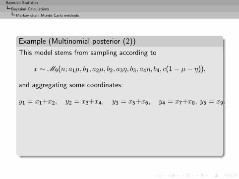
Bayesian Statistics
Bayesian Calculations
Markov chain Monte Carlo methods
Example (Multinomial posterior (2))
This model stems from sampling according to
x ∼ M9(n; a1µ, b1, a2µ, b2, a3η, b3, a4η, b4, c(1 − µ− η)),
and aggregating some coordinates:
y1 = x1+x2, y2 = x3+x4, y3 = x5+x6, y4 = x7+x8, y5 = x9.
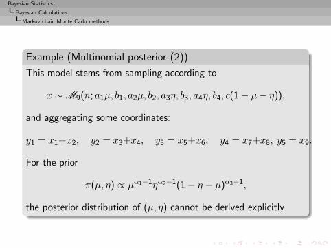
For the prior
π(µ, η) ∝ µα1−1ηα2−1(1 − η − µ)α3−1,
the posterior distribution of (µ, η) cannot be derived explicitly.
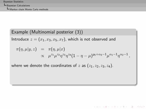
Bayesian Statistics
Bayesian Calculations
Markov chain Monte Carlo methods
Example (Multinomial posterior (3))
Introduce z = (x1, x3, x5, x7), which is not observed and
π(η, µ|y, z) = π(η, µ|x)∝ µz1µz2ηz3ηz4(1 − η − µ)y5+α3−1µα1−1ηα2−1 ,
where we denote the coordinates of z as (z1, z2, z3, z4).
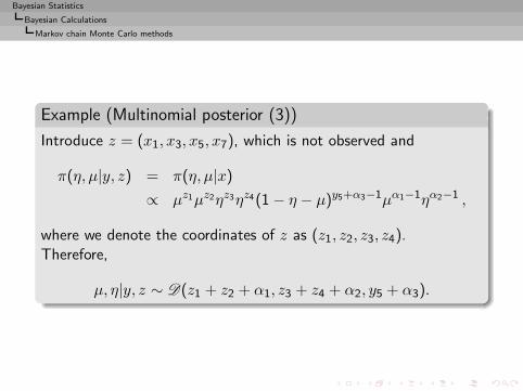
Bayesian Statistics
Bayesian Calculations
Markov chain Monte Carlo methods
Example (Multinomial posterior (3))
Introduce z = (x1, x3, x5, x7), which is not observed and
π(η, µ|y, z) = π(η, µ|x)∝ µz1µz2ηz3ηz4(1 − η − µ)y5+α3−1µα1−1ηα2−1 ,
where we denote the coordinates of z as (z1, z2, z3, z4).Therefore,
µ, η|y, z ∼ D(z1 + z2 + α1, z3 + z4 + α2, y5 + α3).
Bayesian Statistics
Bayesian Calculations
Markov chain Monte Carlo methods
The impact on Bayesian Statistics
◮ Radical modification of the way people work with models andprior assumptions
◮ Allows for much more complex structures:◮ use of graphical models◮ exploration of latent variable models
◮ Removes the need for analytical processing
◮ Boosted hierarchical modeling
◮ Enables (truly) Bayesian model choice
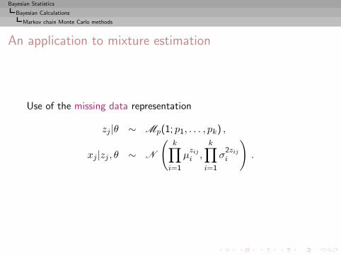
Bayesian Statistics
Bayesian Calculations
Markov chain Monte Carlo methods
An application to mixture estimation
Use of the missing data representation
zj |θ ∼ Mp(1; p1, . . . , pk) ,
xj |zj , θ ∼ N
(k∏
i=1
µzij
i ,
k∏
i=1
σ2zij
i
)
.
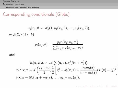
Bayesian Statistics
Bayesian Calculations
Markov chain Monte Carlo methods
Corresponding conditionals (Gibbs)
zj |xj , θ ∼ Mk(1; p1(xj , θ), . . . , pk(xj , θ)),
with (1 ≤ i ≤ k)
pi(xj , θ) =piϕ(xj ;µi, σi)∑kt=1 ptϕ(xj ;µt, σt)
and
µi|x, z, σi ∼ N (ξi(x, z), σ2i /(n + σ2
i )),
σ−2i |x, z ∼ G
(νi + ni
2,1
2
[s2i + s2i (x, z) +
nimi(z)
ni +mi(z)(xi(z) − ξi)
2
])
p|x, z ∼ Dk(α1 +m1(z), . . . , αk +mk(z)),
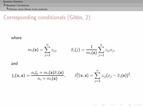
Bayesian Statistics
Bayesian Calculations
Markov chain Monte Carlo methods
Corresponding conditionals (Gibbs, 2)
where
mi(z) =
n∑
j=1
zij , xi(j) =1
mi(z)
n∑
j=1
zijxj ,
and
ξi(x, z) =niξi +mi(z)xi(z)
ni +mi(z), s2i (x, z) =
n∑
j=1
zij(xj − xi(z))2.

Bayesian Statistics
Bayesian Calculations
Markov chain Monte Carlo methods
Properties
◮ Slow moves sometimes
◮ Large increase in dimension, order O(n)
◮ Good theoretical properties (Duality principle)
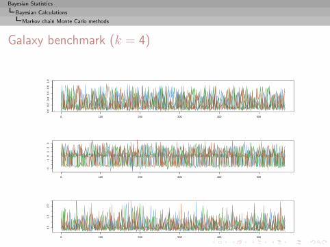
Bayesian Statistics
Bayesian Calculations
Markov chain Monte Carlo methods
Galaxy benchmark (k = 4)
0 100 200 300 400 500
0.0
0.2
0.4
0.6
0.8
1.0
0 100 200 300 400 500
−3
−1
01
23
0 100 200 300 400 500
0.5
1.5
2.5

Bayesian Statistics
Bayesian Calculations
Markov chain Monte Carlo methods
Galaxy benchmark (k = 4)
Average density
data
Rel
ativ
e F
requ
ency
−2 −1 0 1 2 3
0.0
0.2
0.4
0.6
0.8
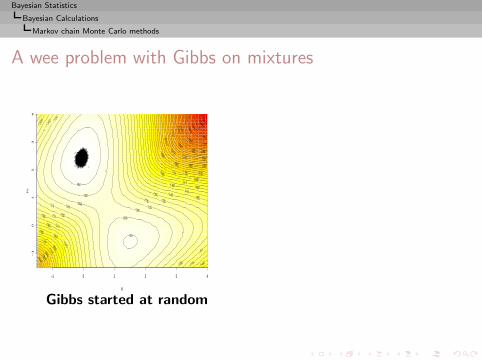
Bayesian Statistics
Bayesian Calculations
Markov chain Monte Carlo methods
A wee problem with Gibbs on mixtures
−1 0 1 2 3 4
−1
01
23
4
µ1
µ2
Gibbs started at random
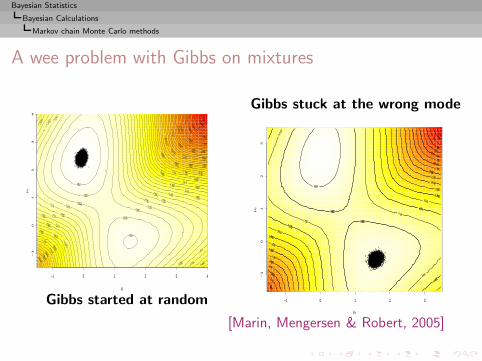
Bayesian Statistics
Bayesian Calculations
Markov chain Monte Carlo methods
A wee problem with Gibbs on mixtures
−1 0 1 2 3 4
−1
01
23
4
µ1
µ2
Gibbs started at random
Gibbs stuck at the wrong mode
−1 0 1 2 3
−1
01
23
µ1
µ2
[Marin, Mengersen & Robert, 2005]
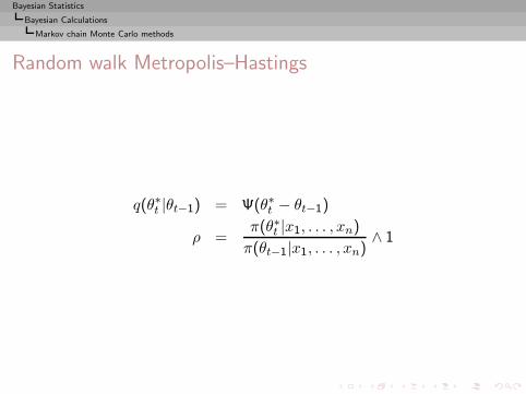
Bayesian Statistics
Bayesian Calculations
Markov chain Monte Carlo methods
Random walk Metropolis–Hastings
q(θ∗t |θt−1) = Ψ(θ∗t − θt−1)
ρ =π(θ∗t |x1, . . . , xn)
π(θt−1|x1, . . . , xn)∧ 1
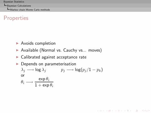
Bayesian Statistics
Bayesian Calculations
Markov chain Monte Carlo methods
Properties
◮ Avoids completion
◮ Available (Normal vs. Cauchy vs... moves)
◮ Calibrated against acceptance rate
◮ Depends on parameterisationλj −→ log λj pj −→ log(pj/1 − pk)or
θi −→exp θi
1 + exp θi
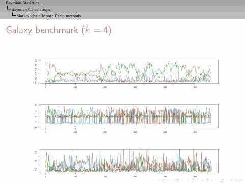
Bayesian Statistics
Bayesian Calculations
Markov chain Monte Carlo methods
Galaxy benchmark (k = 4)
0 100 200 300 400 500
0.0
0.2
0.4
0.6
0.8
1.0
0 100 200 300 400 500
−4
−2
02
4
0 100 200 300 400 500
0.5
1.5
2.5
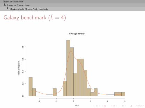
Bayesian Statistics
Bayesian Calculations
Markov chain Monte Carlo methods
Galaxy benchmark (k = 4)
Average density
data
Rel
ativ
e F
requ
ency
−2 −1 0 1 2 3
0.0
0.2
0.4
0.6
0.8
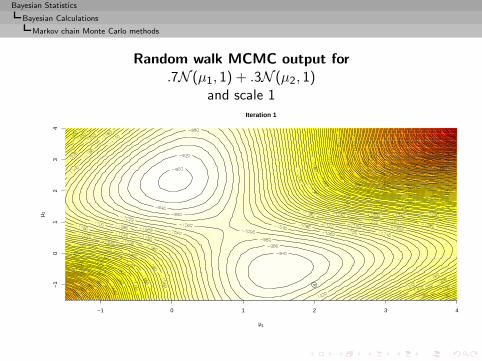
Bayesian Statistics
Bayesian Calculations
Markov chain Monte Carlo methods
Random walk MCMC output for.7N (µ1, 1) + .3N (µ2, 1)
and scale 1
−1 0 1 2 3 4
−1
01
23
4
µ1
µ 2
Iteration 1

Bayesian Statistics
Bayesian Calculations
Markov chain Monte Carlo methods
Random walk MCMC output for.7N (µ1, 1) + .3N (µ2, 1)
and scale 1
−1 0 1 2 3 4
−1
01
23
4
µ1
µ 2
Iteration 10
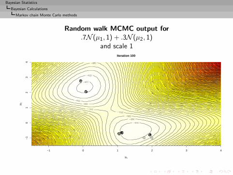
Bayesian Statistics
Bayesian Calculations
Markov chain Monte Carlo methods
Random walk MCMC output for.7N (µ1, 1) + .3N (µ2, 1)
and scale 1
−1 0 1 2 3 4
−1
01
23
4
µ1
µ 2
Iteration 100
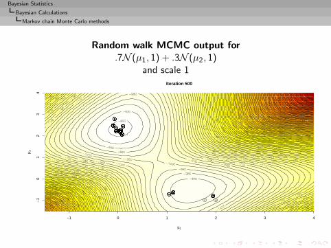
Bayesian Statistics
Bayesian Calculations
Markov chain Monte Carlo methods
Random walk MCMC output for.7N (µ1, 1) + .3N (µ2, 1)
and scale 1
−1 0 1 2 3 4
−1
01
23
4
µ1
µ 2
Iteration 500
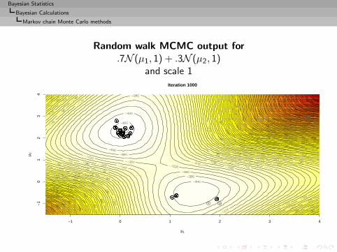
Bayesian Statistics
Bayesian Calculations
Markov chain Monte Carlo methods
Random walk MCMC output for.7N (µ1, 1) + .3N (µ2, 1)
and scale 1
−1 0 1 2 3 4
−1
01
23
4
µ1
µ 2
Iteration 1000
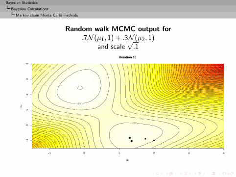
Bayesian Statistics
Bayesian Calculations
Markov chain Monte Carlo methods
Random walk MCMC output for.7N (µ1, 1) + .3N (µ2, 1)
and scale√.1
−1 0 1 2 3 4
−1
01
23
4
µ1
µ 2
Iteration 10
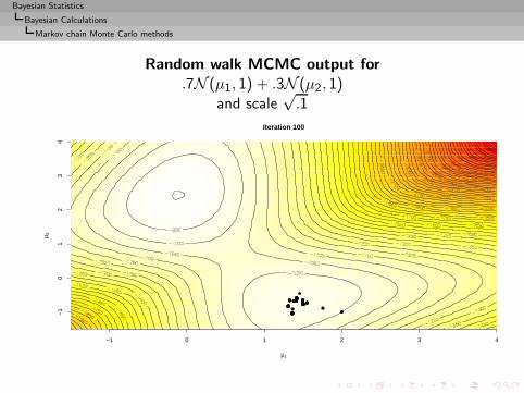
Bayesian Statistics
Bayesian Calculations
Markov chain Monte Carlo methods
Random walk MCMC output for.7N (µ1, 1) + .3N (µ2, 1)
and scale√.1
−1 0 1 2 3 4
−1
01
23
4
µ1
µ 2
Iteration 100
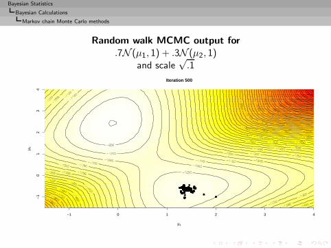
Bayesian Statistics
Bayesian Calculations
Markov chain Monte Carlo methods
Random walk MCMC output for.7N (µ1, 1) + .3N (µ2, 1)
and scale√.1
−1 0 1 2 3 4
−1
01
23
4
µ1
µ 2
Iteration 500
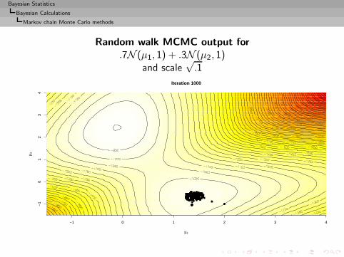
Bayesian Statistics
Bayesian Calculations
Markov chain Monte Carlo methods
Random walk MCMC output for.7N (µ1, 1) + .3N (µ2, 1)
and scale√.1
−1 0 1 2 3 4
−1
01
23
4
µ1
µ 2
Iteration 1000
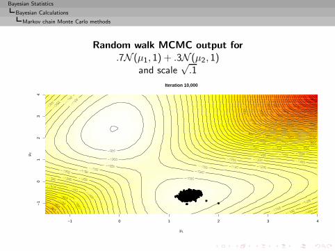
Bayesian Statistics
Bayesian Calculations
Markov chain Monte Carlo methods
Random walk MCMC output for.7N (µ1, 1) + .3N (µ2, 1)
and scale√.1
−1 0 1 2 3 4
−1
01
23
4
µ1
µ 2
Iteration 10,000

Bayesian Statistics
Bayesian Calculations
Markov chain Monte Carlo methods
Random walk MCMC output for.7N (µ1, 1) + .3N (µ2, 1)
and scale√.1
−1 0 1 2 3 4
−1
01
23
4
µ1
µ 2
Iteration 5000
Bayesian Statistics
Tests and model choice
Tests and model choice
Introduction
Decision-Theoretic Foundations of Statistical Inference
From Prior Information to Prior Distributions
Bayesian Point Estimation
Bayesian Calculations
Tests and model choiceBayesian testsBayes factorsPseudo-Bayes factorsIntrinsic priors
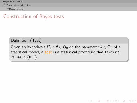
Bayesian Statistics
Tests and model choice
Bayesian tests
Construction of Bayes tests
Definition (Test)
Given an hypothesis H0 : θ ∈ Θ0 on the parameter θ ∈ Θ0 of astatistical model, a test is a statistical procedure that takes itsvalues in {0, 1}.
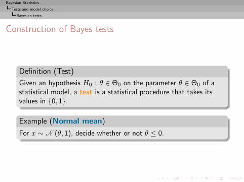
Bayesian Statistics
Tests and model choice
Bayesian tests
Construction of Bayes tests
Definition (Test)
Given an hypothesis H0 : θ ∈ Θ0 on the parameter θ ∈ Θ0 of astatistical model, a test is a statistical procedure that takes itsvalues in {0, 1}.
Example (Normal mean)
For x ∼ N (θ, 1), decide whether or not θ ≤ 0.
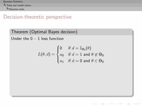
Bayesian Statistics
Tests and model choice
Bayesian tests
Decision-theoretic perspective
Theorem (Optimal Bayes decision)
Under the 0 − 1 loss function
L(θ, d) =
0 if d = IΘ0(θ)
a0 if d = 1 and θ 6∈ Θ0
a1 if d = 0 and θ ∈ Θ0
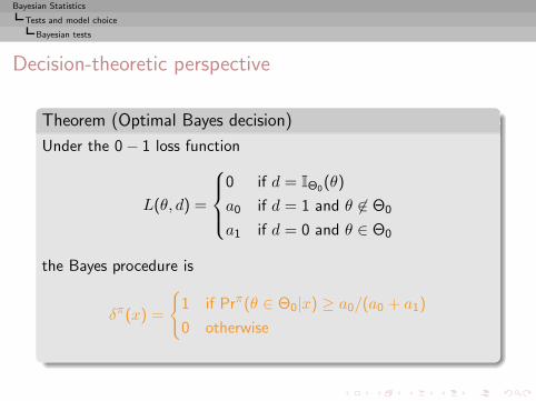
Bayesian Statistics
Tests and model choice
Bayesian tests
Decision-theoretic perspective
Theorem (Optimal Bayes decision)
Under the 0 − 1 loss function
L(θ, d) =
0 if d = IΘ0(θ)
a0 if d = 1 and θ 6∈ Θ0
a1 if d = 0 and θ ∈ Θ0
the Bayes procedure is
δπ(x) =
{1 if Prπ(θ ∈ Θ0|x) ≥ a0/(a0 + a1)
0 otherwise
Bayesian Statistics
Tests and model choice
Bayesian tests
Bound comparison
Determination of a0/a1 depends on consequences of “wrongdecision” under both circumstances
Bayesian Statistics
Tests and model choice
Bayesian tests
Bound comparison
Determination of a0/a1 depends on consequences of “wrongdecision” under both circumstancesOften difficult to assess in practice and replacement with “golden”bounds like .05, biased towards H0
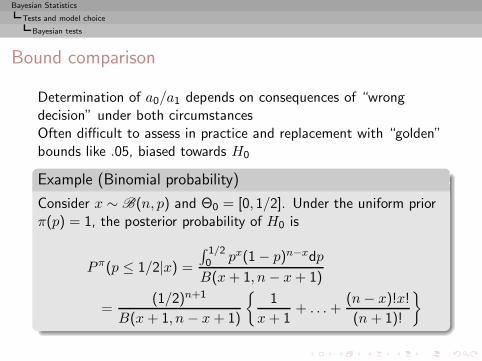
Bayesian Statistics
Tests and model choice
Bayesian tests
Bound comparison
Determination of a0/a1 depends on consequences of “wrongdecision” under both circumstancesOften difficult to assess in practice and replacement with “golden”bounds like .05, biased towards H0
Example (Binomial probability)
Consider x ∼ B(n, p) and Θ0 = [0, 1/2]. Under the uniform priorπ(p) = 1, the posterior probability of H0 is
P π(p ≤ 1/2|x) =
∫ 1/20 px(1 − p)n−xdp
B(x+ 1, n− x+ 1)
=(1/2)n+1
B(x+ 1, n − x+ 1)
{1
x+ 1+ . . .+
(n− x)!x!
(n + 1)!
}
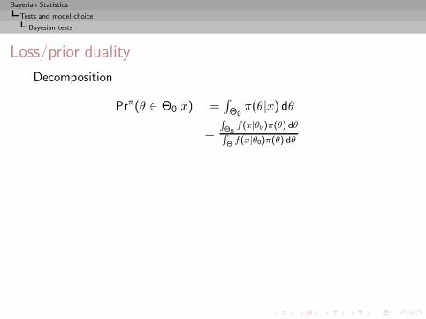
Bayesian Statistics
Tests and model choice
Bayesian tests
Loss/prior duality
Decomposition
Prπ(θ ∈ Θ0|x) =∫Θ0π(θ|x) dθ
=
R
Θ0f(x|θ0)π(θ) dθ
R
Θ f(x|θ0)π(θ) dθ
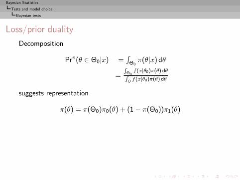
Bayesian Statistics
Tests and model choice
Bayesian tests
Loss/prior duality
Decomposition
Prπ(θ ∈ Θ0|x) =∫Θ0π(θ|x) dθ
=
R
Θ0f(x|θ0)π(θ) dθ
R
Θ f(x|θ0)π(θ) dθ
suggests representation
π(θ) = π(Θ0)π0(θ) + (1 − π(Θ0))π1(θ)
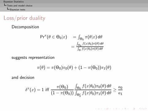
Bayesian Statistics
Tests and model choice
Bayesian tests
Loss/prior duality
Decomposition
Prπ(θ ∈ Θ0|x) =∫Θ0π(θ|x) dθ
=
R
Θ0f(x|θ0)π(θ) dθ
R
Θ f(x|θ0)π(θ) dθ
suggests representation
π(θ) = π(Θ0)π0(θ) + (1 − π(Θ0))π1(θ)
and decision
δπ(x) = 1 iffπ(Θ0)
(1 − π(Θ0))
∫Θ0f(x|θ0)π0(θ) dθ
∫Θc
0f(x|θ0)π1(θ) dθ
≥ a0
a1
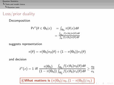
c©What matters is (π(Θ0)/a0, (1 − π(Θ0))/a1)
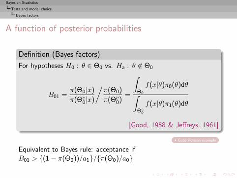
Bayesian Statistics
Tests and model choice
Bayes factors
A function of posterior probabilities
Definition (Bayes factors)
For hypotheses H0 : θ ∈ Θ0 vs. Ha : θ 6∈ Θ0
B01 =π(Θ0|x)π(Θc
0|x)
/π(Θ0)
π(Θc0)
=
∫
Θ0
f(x|θ)π0(θ)dθ
∫
Θc0
f(x|θ)π1(θ)dθ
[Good, 1958 & Jeffreys, 1961]
Goto Poisson example
Equivalent to Bayes rule: acceptance ifB01 > {(1 − π(Θ0))/a1}/{π(Θ0)/a0}

Bayesian Statistics
Tests and model choice
Bayes factors
Self-contained concept
Outside decision-theoretic environment:
◮ eliminates choice of π(Θ0)

Bayesian Statistics
Tests and model choice
Bayes factors
Self-contained concept
Outside decision-theoretic environment:
◮ eliminates choice of π(Θ0)
◮ but depends on the choice of (π0, π1)
Bayesian Statistics
Tests and model choice
Bayes factors
Self-contained concept
Outside decision-theoretic environment:
◮ eliminates choice of π(Θ0)
◮ but depends on the choice of (π0, π1)
◮ Bayesian/marginal equivalent to the likelihood ratio

Bayesian Statistics
Tests and model choice
Bayes factors
Self-contained concept
Outside decision-theoretic environment:
◮ eliminates choice of π(Θ0)
◮ but depends on the choice of (π0, π1)
◮ Bayesian/marginal equivalent to the likelihood ratio
◮ Jeffreys’ scale of evidence:◮ if log10(B
π10) between 0 and 0.5, evidence against H0 weak,
◮ if log10(Bπ10) 0.5 and 1, evidence substantial,
◮ if log10(Bπ10) 1 and 2, evidence strong and
◮ if log10(Bπ10) above 2, evidence decisive
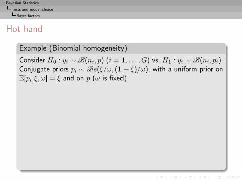
Bayesian Statistics
Tests and model choice
Bayes factors
Hot hand
Example (Binomial homogeneity)
Consider H0 : yi ∼ B(ni, p) (i = 1, . . . , G) vs. H1 : yi ∼ B(ni, pi).Conjugate priors pi ∼ Be(ξ/ω, (1 − ξ)/ω), with a uniform prior onE[pi|ξ, ω] = ξ and on p (ω is fixed)
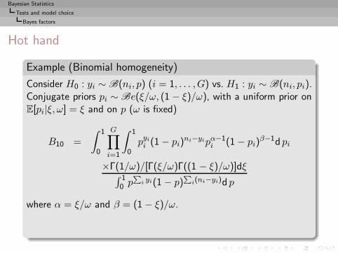
Bayesian Statistics
Tests and model choice
Bayes factors
Hot hand
Example (Binomial homogeneity)
Consider H0 : yi ∼ B(ni, p) (i = 1, . . . , G) vs. H1 : yi ∼ B(ni, pi).Conjugate priors pi ∼ Be(ξ/ω, (1 − ξ)/ω), with a uniform prior onE[pi|ξ, ω] = ξ and on p (ω is fixed)
B10 =
∫ 1
0
G∏
i=1
∫ 1
0pyi
i (1 − pi)ni−yipα−1
i (1 − pi)β−1d pi
×Γ(1/ω)/[Γ(ξ/ω)Γ((1 − ξ)/ω)]dξ∫ 10 p
P
i yi(1 − p)P
i(ni−yi)d p
where α = ξ/ω and β = (1 − ξ)/ω.
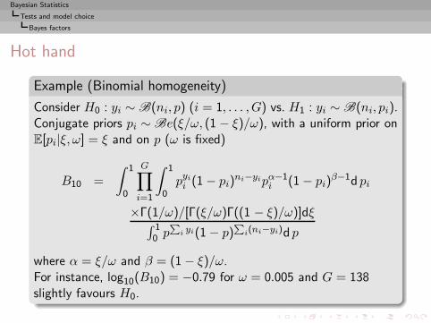
Bayesian Statistics
Tests and model choice
Bayes factors
Hot hand
Example (Binomial homogeneity)
Consider H0 : yi ∼ B(ni, p) (i = 1, . . . , G) vs. H1 : yi ∼ B(ni, pi).Conjugate priors pi ∼ Be(ξ/ω, (1 − ξ)/ω), with a uniform prior onE[pi|ξ, ω] = ξ and on p (ω is fixed)
B10 =
∫ 1
0
G∏
i=1
∫ 1
0pyi
i (1 − pi)ni−yipα−1
i (1 − pi)β−1d pi
×Γ(1/ω)/[Γ(ξ/ω)Γ((1 − ξ)/ω)]dξ∫ 10 p
P
i yi(1 − p)P
i(ni−yi)d p
where α = ξ/ω and β = (1 − ξ)/ω.For instance, log10(B10) = −0.79 for ω = 0.005 and G = 138slightly favours H0.

Bayesian Statistics
Tests and model choice
Bayes factors
A major modification
When the null hypothesis is supported by a set of measure 0,π(Θ0) = 0
[End of the story?!]
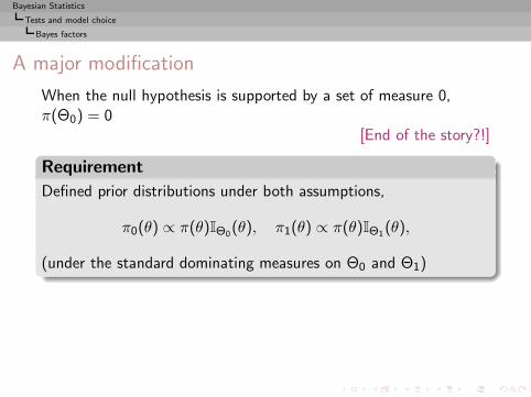
Bayesian Statistics
Tests and model choice
Bayes factors
A major modification
When the null hypothesis is supported by a set of measure 0,π(Θ0) = 0
[End of the story?!]
Requirement
Defined prior distributions under both assumptions,
π0(θ) ∝ π(θ)IΘ0(θ), π1(θ) ∝ π(θ)IΘ1
(θ),
(under the standard dominating measures on Θ0 and Θ1)
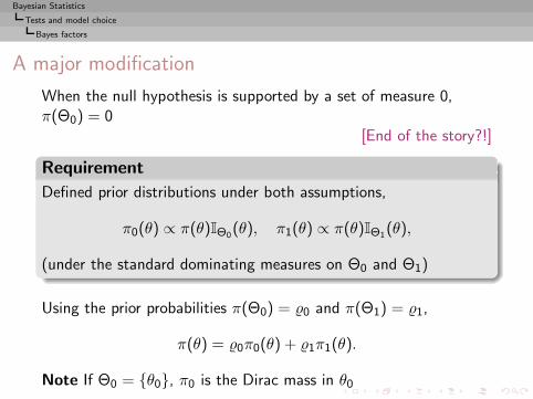
Using the prior probabilities π(Θ0) = 0 and π(Θ1) = 1,
π(θ) = 0π0(θ) + 1π1(θ).
Note If Θ0 = {θ0}, π0 is the Dirac mass in θ0
Bayesian Statistics
Tests and model choice
Bayes factors
Point null hypotheses
Particular case H0 : θ = θ0Take ρ0 = Prπ(θ = θ0) and g1 prior density under Ha.
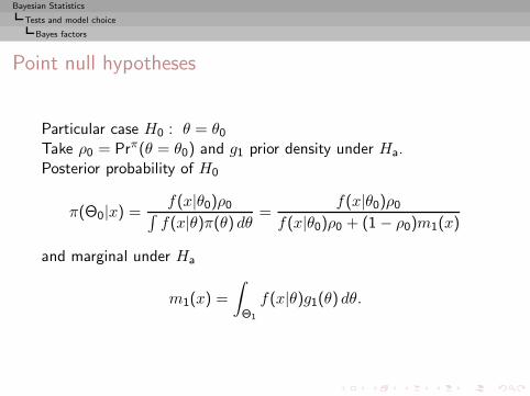
Bayesian Statistics
Tests and model choice
Bayes factors
Point null hypotheses
Particular case H0 : θ = θ0Take ρ0 = Prπ(θ = θ0) and g1 prior density under Ha.Posterior probability of H0
π(Θ0|x) =f(x|θ0)ρ0∫f(x|θ)π(θ) dθ
=f(x|θ0)ρ0
f(x|θ0)ρ0 + (1 − ρ0)m1(x)
and marginal under Ha
m1(x) =
∫
Θ1
f(x|θ)g1(θ) dθ.
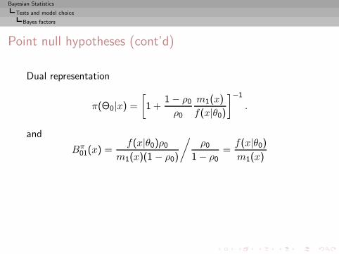
Bayesian Statistics
Tests and model choice
Bayes factors
Point null hypotheses (cont’d)
Dual representation
π(Θ0|x) =
[1 +
1 − ρ0
ρ0
m1(x)
f(x|θ0)
]−1
.
and
Bπ01(x) =
f(x|θ0)ρ0
m1(x)(1 − ρ0)
/ρ0
1 − ρ0=f(x|θ0)m1(x)
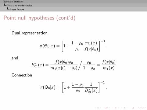
Bayesian Statistics
Tests and model choice
Bayes factors
Point null hypotheses (cont’d)
Dual representation
π(Θ0|x) =
[1 +
1 − ρ0
ρ0
m1(x)
f(x|θ0)
]−1
.
and
Bπ01(x) =
f(x|θ0)ρ0
m1(x)(1 − ρ0)
/ρ0
1 − ρ0=f(x|θ0)m1(x)
Connection
π(Θ0|x) =
[1 +
1 − ρ0
ρ0
1
Bπ01(x)
]−1
.
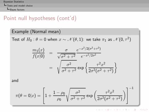
Bayesian Statistics
Tests and model choice
Bayes factors
Point null hypotheses (cont’d)
Example (Normal mean)
Test of H0 : θ = 0 when x ∼ N (θ, 1): we take π1 as N (0, τ2)
m1(x)
f(x|0) =σ√
σ2 + τ2
e−x2/2(σ2+τ2)
e−x2/2σ2
=
√σ2
σ2 + τ2exp
{τ2x2
2σ2(σ2 + τ2)
}
and
π(θ = 0|x) =
1 +1 − ρ0
ρ0
√σ2
σ2 + τ2exp
(τ2x2
2σ2(σ2 + τ2)
)
−1
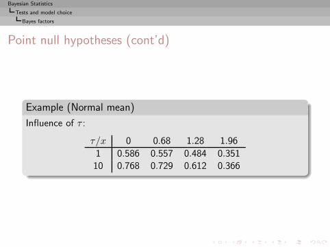
Bayesian Statistics
Tests and model choice
Bayes factors
Point null hypotheses (cont’d)
Example (Normal mean)
Influence of τ :
τ/x 0 0.68 1.28 1.96
1 0.586 0.557 0.484 0.35110 0.768 0.729 0.612 0.366
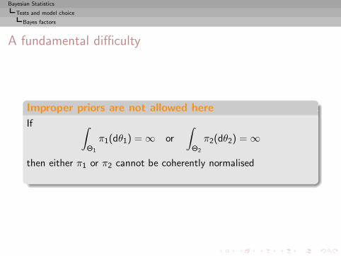
Bayesian Statistics
Tests and model choice
Bayes factors
A fundamental difficulty
Improper priors are not allowed here
If ∫
Θ1
π1(dθ1) = ∞ or
∫
Θ2
π2(dθ2) = ∞
then either π1 or π2 cannot be coherently normalised
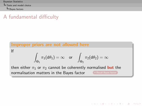
Bayesian Statistics
Tests and model choice
Bayes factors
A fundamental difficulty
Improper priors are not allowed here
If ∫
Θ1
π1(dθ1) = ∞ or
∫
Θ2
π2(dθ2) = ∞
then either π1 or π2 cannot be coherently normalised but thenormalisation matters in the Bayes factor Recall Bayes factor
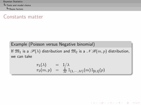
Bayesian Statistics
Tests and model choice
Bayes factors
Constants matter
Example (Poisson versus Negative binomial)
If M1 is a P(λ) distribution and M2 is a N B(m,p) distribution,we can take
π1(λ) = 1/λπ2(m, p) = 1
M I{1,··· ,M}(m) I[0,1](p)
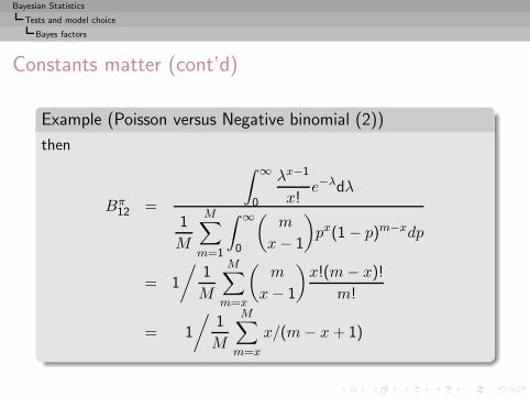
Bayesian Statistics
Tests and model choice
Bayes factors
Constants matter (cont’d)
Example (Poisson versus Negative binomial (2))
then
Bπ12 =
∫ ∞
0
λx−1
x!e−λdλ
1
M
M∑
m=1
∫ ∞
0
(m
x− 1
)px(1 − p)m−xdp
= 1
/1
M
M∑
m=x
(m
x− 1
)x!(m− x)!
m!
= 1
/1
M
M∑
m=x
x/(m− x+ 1)
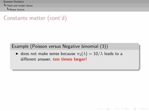
Bayesian Statistics
Tests and model choice
Bayes factors
Constants matter (cont’d)
Example (Poisson versus Negative binomial (3))
◮ does not make sense because π1(λ) = 10/λ leads to adifferent answer, ten times larger!
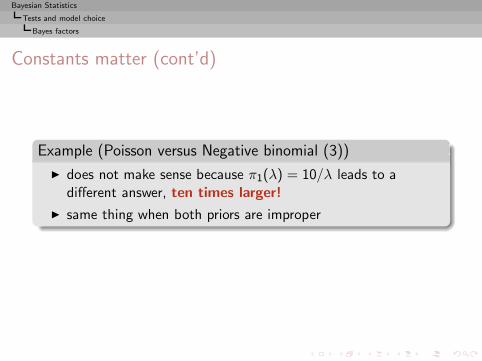
Bayesian Statistics
Tests and model choice
Bayes factors
Constants matter (cont’d)
Example (Poisson versus Negative binomial (3))
◮ does not make sense because π1(λ) = 10/λ leads to adifferent answer, ten times larger!
◮ same thing when both priors are improper
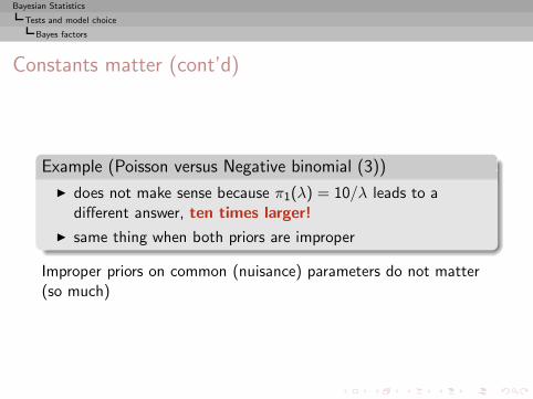
Bayesian Statistics
Tests and model choice
Bayes factors
Constants matter (cont’d)
Example (Poisson versus Negative binomial (3))
◮ does not make sense because π1(λ) = 10/λ leads to adifferent answer, ten times larger!
◮ same thing when both priors are improper
Improper priors on common (nuisance) parameters do not matter(so much)
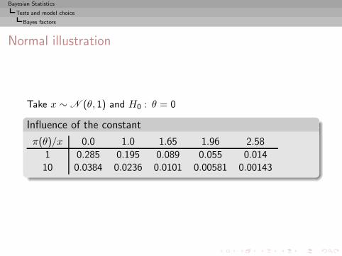
Bayesian Statistics
Tests and model choice
Bayes factors
Normal illustration
Take x ∼ N (θ, 1) and H0 : θ = 0
Influence of the constant
π(θ)/x 0.0 1.0 1.65 1.96 2.58
1 0.285 0.195 0.089 0.055 0.01410 0.0384 0.0236 0.0101 0.00581 0.00143

Bayesian Statistics
Tests and model choice
Bayes factors
Vague proper priors are not the solution
Taking a proper prior and take a “very large” variance (e.g.,BUGS)

Bayesian Statistics
Tests and model choice
Bayes factors
Vague proper priors are not the solution
Taking a proper prior and take a “very large” variance (e.g.,BUGS) will most often result in an undefined or ill-defined limit
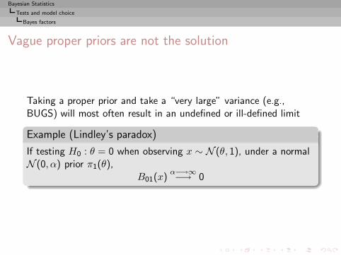
Bayesian Statistics
Tests and model choice
Bayes factors
Vague proper priors are not the solution
Taking a proper prior and take a “very large” variance (e.g.,BUGS) will most often result in an undefined or ill-defined limit
Example (Lindley’s paradox)
If testing H0 : θ = 0 when observing x ∼ N (θ, 1), under a normalN (0, α) prior π1(θ),
B01(x)α−→∞−→ 0
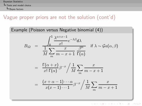
Bayesian Statistics
Tests and model choice
Bayes factors
Vague proper priors are not the solution (cont’d)
Example (Poisson versus Negative binomial (4))
B12 =
∫ 1
0
λα+x−1
x!e−λβdλ
1
M
∑
m
x
m− x+ 1
βα
Γ(α)
if λ ∼ Ga(α, β)
=Γ(α+ x)
x! Γ(α)β−x
/1
M
∑
m
x
m− x+ 1
=(x+ α− 1) · · ·αx(x− 1) · · · 1 β−x
/1
M
∑
m
x
m− x+ 1
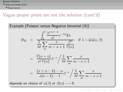
depends on choice of α(β) or β(α) −→ 0
Bayesian Statistics
Tests and model choice
Bayes factors
Learning from the sample
Definition (Learning sample)
Given an improper prior π, (x1, . . . , xn) is a learning sample ifπ(·|x1, . . . , xn) is proper and a minimal learning sample if none ofits subsamples is a learning sample
Bayesian Statistics
Tests and model choice
Bayes factors
Learning from the sample
Definition (Learning sample)
Given an improper prior π, (x1, . . . , xn) is a learning sample ifπ(·|x1, . . . , xn) is proper and a minimal learning sample if none ofits subsamples is a learning sample
There is just enough information in a minimal learning sample tomake inference about θ under the prior π

Bayesian Statistics
Tests and model choice
Pseudo-Bayes factors
Pseudo-Bayes factors
Idea
Use one part x[i] of the data x to make the prior proper:
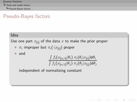
Bayesian Statistics
Tests and model choice
Pseudo-Bayes factors
Pseudo-Bayes factors
Idea
Use one part x[i] of the data x to make the prior proper:
◮ πi improper but πi(·|x[i]) proper
◮ and ∫fi(x[n/i]|θi) πi(θi|x[i])dθi∫fj(x[n/i]|θj) πj(θj|x[i])dθj
independent of normalizing constant
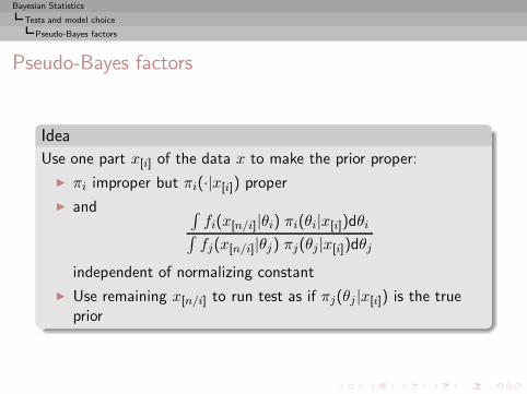
Bayesian Statistics
Tests and model choice
Pseudo-Bayes factors
Pseudo-Bayes factors
Idea
Use one part x[i] of the data x to make the prior proper:
◮ πi improper but πi(·|x[i]) proper
◮ and ∫fi(x[n/i]|θi) πi(θi|x[i])dθi∫fj(x[n/i]|θj) πj(θj|x[i])dθj
independent of normalizing constant
◮ Use remaining x[n/i] to run test as if πj(θj |x[i]) is the trueprior

Bayesian Statistics
Tests and model choice
Pseudo-Bayes factors
Motivation
◮ Provides a working principle for improper priors

Bayesian Statistics
Tests and model choice
Pseudo-Bayes factors
Motivation
◮ Provides a working principle for improper priors
◮ Gather enough information from data to achieve properness
◮ and use this properness to run the test on remaining data
Bayesian Statistics
Tests and model choice
Pseudo-Bayes factors
Motivation
◮ Provides a working principle for improper priors
◮ Gather enough information from data to achieve properness
◮ and use this properness to run the test on remaining data
◮ does not use x twice as in Aitkin’s (1991)
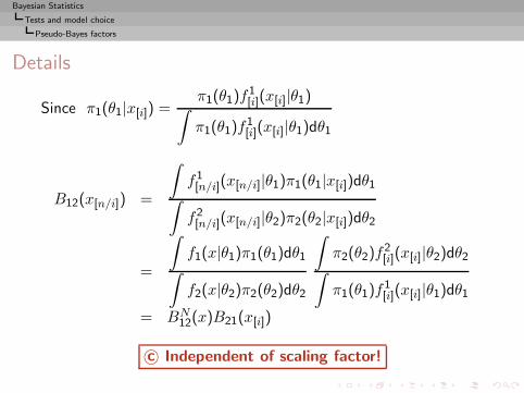
Bayesian Statistics
Tests and model choice
Pseudo-Bayes factors
Details
Since π1(θ1|x[i]) =π1(θ1)f
1[i](x[i]|θ1)∫
π1(θ1)f1[i](x[i]|θ1)dθ1
B12(x[n/i]) =
∫f1[n/i](x[n/i]|θ1)π1(θ1|x[i])dθ1
∫f2[n/i](x[n/i]|θ2)π2(θ2|x[i])dθ2
=
∫f1(x|θ1)π1(θ1)dθ1
∫f2(x|θ2)π2(θ2)dθ2
∫π2(θ2)f
2[i](x[i]|θ2)dθ2
∫π1(θ1)f
1[i](x[i]|θ1)dθ1
= BN12(x)B21(x[i])
c© Independent of scaling factor!

Bayesian Statistics
Tests and model choice
Pseudo-Bayes factors
Unexpected problems!
◮ depends on the choice of x[i]
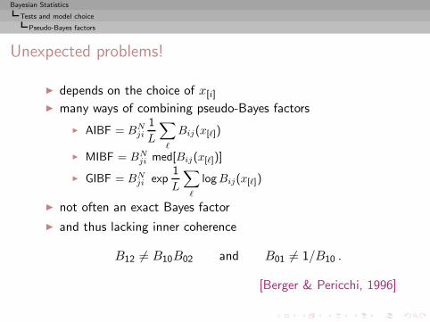
Bayesian Statistics
Tests and model choice
Pseudo-Bayes factors
Unexpected problems!
◮ depends on the choice of x[i]
◮ many ways of combining pseudo-Bayes factors
◮ AIBF = BNji
1
L
∑
ℓ
Bij(x[ℓ])
◮ MIBF = BNji med[Bij(x[ℓ])]
◮ GIBF = BNji exp
1
L
∑
ℓ
logBij(x[ℓ])
◮ not often an exact Bayes factor
◮ and thus lacking inner coherence
B12 6= B10B02 and B01 6= 1/B10 .
[Berger & Pericchi, 1996]
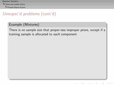
Bayesian Statistics
Tests and model choice
Pseudo-Bayes factors
Unexpec’d problems (cont’d)
Example (Mixtures)
There is no sample size that proper-ises improper priors, except if atraining sample is allocated to each component
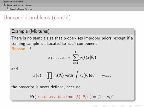
Bayesian Statistics
Tests and model choice
Pseudo-Bayes factors
Unexpec’d problems (cont’d)
Example (Mixtures)
There is no sample size that proper-ises improper priors, except if atraining sample is allocated to each componentReason If
x1, . . . , xn ∼k∑
i=1
pif(x|θi)
and
π(θ) =∏
i
πi(θi) with
∫πi(θi)dθi = +∞ ,
the posterior is never defined, because
Pr(“no observation from f(·|θi)”) = (1 − pi)n

Bayesian Statistics
Tests and model choice
Intrinsic priors
Intrinsic priors
There may exist a true prior that provides the same Bayes factor
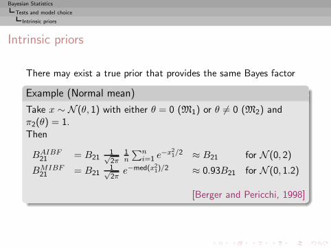
Bayesian Statistics
Tests and model choice
Intrinsic priors
Intrinsic priors
There may exist a true prior that provides the same Bayes factor
Example (Normal mean)
Take x ∼ N (θ, 1) with either θ = 0 (M1) or θ 6= 0 (M2) andπ2(θ) = 1.Then
BAIBF21 = B21
1√2π
1n
∑ni=1 e
−x21/2 ≈ B21 for N (0, 2)
BMIBF21 = B21
1√2πe−med(x2
1)/2 ≈ 0.93B21 for N (0, 1.2)
[Berger and Pericchi, 1998]
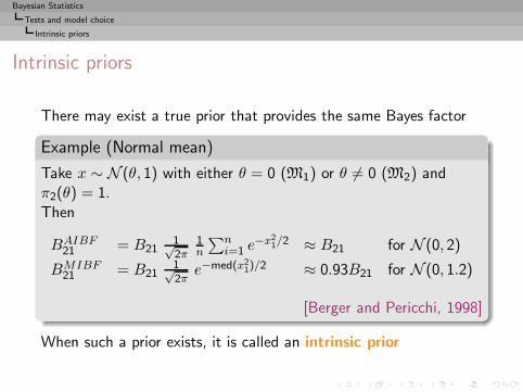
When such a prior exists, it is called an intrinsic prior

Bayesian Statistics
Tests and model choice
Intrinsic priors
Intrinsic priors (cont’d)
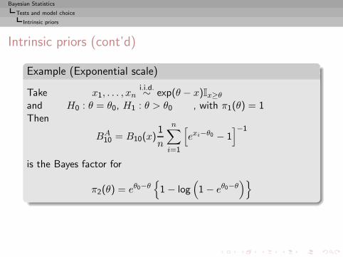
Bayesian Statistics
Tests and model choice
Intrinsic priors
Intrinsic priors (cont’d)
Example (Exponential scale)
Take x1, . . . , xni.i.d.∼ exp(θ − x)Ix≥θ
and H0 : θ = θ0, H1 : θ > θ0 , with π1(θ) = 1Then
BA10 = B10(x)
1
n
n∑
i=1
[exi−θ0 − 1
]−1
is the Bayes factor for
π2(θ) = eθ0−θ{1 − log
(1 − eθ0−θ
)}
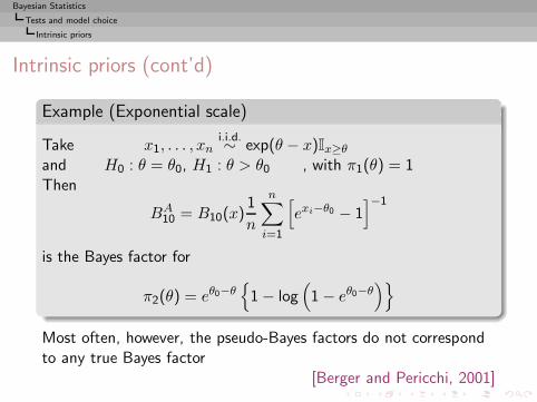
Most often, however, the pseudo-Bayes factors do not correspondto any true Bayes factor
[Berger and Pericchi, 2001]
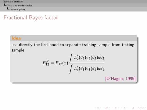
Bayesian Statistics
Tests and model choice
Intrinsic priors
Fractional Bayes factor
Idea
use directly the likelihood to separate training sample from testingsample
BF12 = B12(x)
∫Lb2(θ2)π2(θ2)dθ2
∫Lb1(θ1)π1(θ1)dθ1
[O’Hagan, 1995]
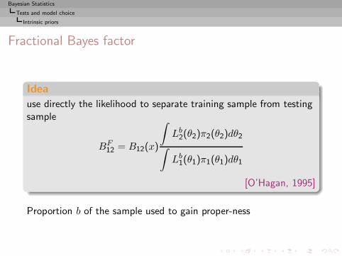
Bayesian Statistics
Tests and model choice
Intrinsic priors
Fractional Bayes factor
Idea
use directly the likelihood to separate training sample from testingsample
BF12 = B12(x)
∫Lb2(θ2)π2(θ2)dθ2
∫Lb1(θ1)π1(θ1)dθ1
[O’Hagan, 1995]
Proportion b of the sample used to gain proper-ness
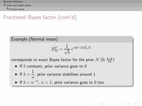
Bayesian Statistics
Tests and model choice
Intrinsic priors
Fractional Bayes factor (cont’d)
Example (Normal mean)
BF12 =
1√ben(b−1)x2
n/2
corresponds to exact Bayes factor for the prior N(0, 1−b
nb
)
◮ If b constant, prior variance goes to 0
◮ If b =1
n, prior variance stabilises around 1
◮ If b = n−α, α < 1, prior variance goes to 0 too.
Bayesian Statistics
Tests and model choice
Opposition to classical tests
Comparison with classical tests
Standard answer
Definition (p-value)
The p-value p(x) associated with a test is the largest significancelevel for which H0 is rejected
Bayesian Statistics
Tests and model choice
Opposition to classical tests
Comparison with classical tests
Standard answer
Definition (p-value)
The p-value p(x) associated with a test is the largest significancelevel for which H0 is rejected
Note
An alternative definition is that a p-value is distributed uniformlyunder the null hypothesis.
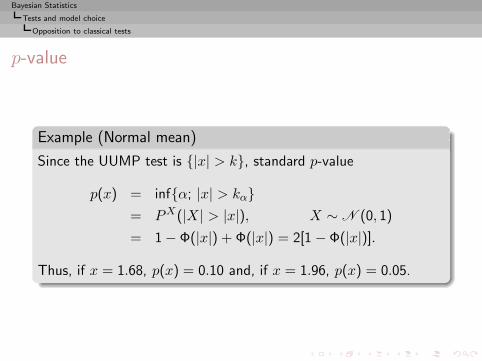
Bayesian Statistics
Tests and model choice
Opposition to classical tests
p-value
Example (Normal mean)
Since the UUMP test is {|x| > k}, standard p-value
p(x) = inf{α; |x| > kα}= PX(|X| > |x|), X ∼ N (0, 1)
= 1 − Φ(|x|) + Φ(|x|) = 2[1 − Φ(|x|)].
Thus, if x = 1.68, p(x) = 0.10 and, if x = 1.96, p(x) = 0.05.
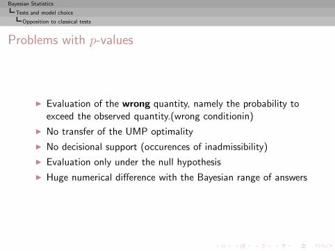
Bayesian Statistics
Tests and model choice
Opposition to classical tests
Problems with p-values
◮ Evaluation of the wrong quantity, namely the probability toexceed the observed quantity.(wrong conditionin)
◮ No transfer of the UMP optimality
◮ No decisional support (occurences of inadmissibility)
◮ Evaluation only under the null hypothesis
◮ Huge numerical difference with the Bayesian range of answers
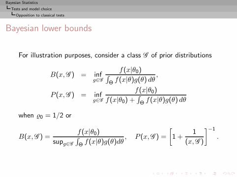
Bayesian Statistics
Tests and model choice
Opposition to classical tests
Bayesian lower bounds
For illustration purposes, consider a class G of prior distributions
B(x,G ) = infg∈G
f(x|θ0)∫Θ f(x|θ)g(θ) dθ ,
P (x,G ) = infg∈G
f(x|θ0)f(x|θ0) +
∫Θ f(x|θ)g(θ) dθ
when 0 = 1/2 or
B(x,G ) =f(x|θ0)
supg∈G
∫Θ f(x|θ)g(θ)dθ , P (x,G ) =
[1 +
1
(x,G )
]−1
.
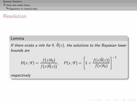
Bayesian Statistics
Tests and model choice
Opposition to classical tests
Resolution
Lemma
If there exists a mle for θ, θ(x), the solutions to the Bayesian lowerbounds are
B(x,G ) =f(x|θ0)f(x|θ(x))
, P (x,G ) =
[
1 +f(x|θ(x))f(x|θ0)
]−1
respectively
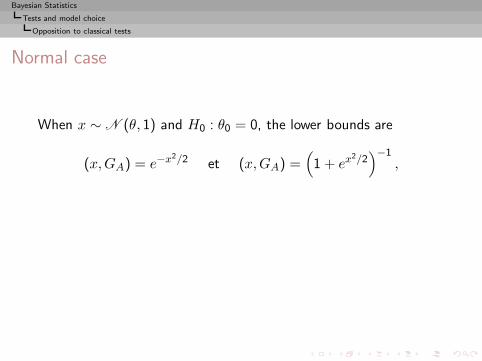
Bayesian Statistics
Tests and model choice
Opposition to classical tests
Normal case
When x ∼ N (θ, 1) and H0 : θ0 = 0, the lower bounds are
(x,GA) = e−x2/2 et (x,GA) =
(1 + ex
2/2)−1
,
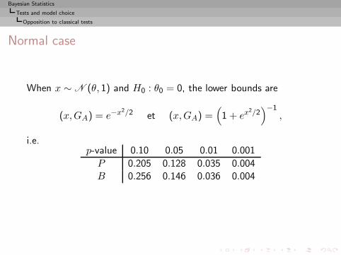
Bayesian Statistics
Tests and model choice
Opposition to classical tests
Normal case
When x ∼ N (θ, 1) and H0 : θ0 = 0, the lower bounds are
(x,GA) = e−x2/2 et (x,GA) =
(1 + ex
2/2)−1
,
i.e.p-value 0.10 0.05 0.01 0.001
P 0.205 0.128 0.035 0.004B 0.256 0.146 0.036 0.004

Bayesian Statistics
Tests and model choice
Opposition to classical tests
Normal case
When x ∼ N (θ, 1) and H0 : θ0 = 0, the lower bounds are
(x,GA) = e−x2/2 et (x,GA) =
(1 + ex
2/2)−1
,
i.e.p-value 0.10 0.05 0.01 0.001
P 0.205 0.128 0.035 0.004B 0.256 0.146 0.036 0.004
[Quite different!]
Bayesian Statistics
Tests and model choice
Opposition to classical tests
Unilateral case
Different situation when H0 : θ ≤ 0
Bayesian Statistics
Tests and model choice
Opposition to classical tests
Unilateral case
Different situation when H0 : θ ≤ 0
◮ Single prior can be used both for H0 and Ha
Bayesian Statistics
Tests and model choice
Opposition to classical tests
Unilateral case
Different situation when H0 : θ ≤ 0
◮ Single prior can be used both for H0 and Ha
◮ Improper priors are therefore acceptable
Bayesian Statistics
Tests and model choice
Opposition to classical tests
Unilateral case
Different situation when H0 : θ ≤ 0
◮ Single prior can be used both for H0 and Ha
◮ Improper priors are therefore acceptable
◮ Similar numerical values compared with p-values
Bayesian Statistics
Tests and model choice
Opposition to classical tests
Unilateral agreement
Theorem
When x ∼ f(x− θ), with f symmetric around 0 and endowed withthe monotone likelihood ratio property, if H0 : θ ≤ 0, the p-valuep(x) is equal to the lower bound of the posterior probabilities,P (x,GSU ), when GSU is the set of symmetric unimodal priors andwhen x > 0.
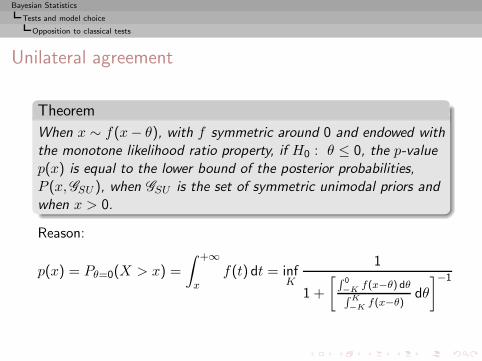
Reason:
p(x) = Pθ=0(X > x) =
∫ +∞
xf(t) dt = inf
K
1
1 +
[R 0−K
f(x−θ) dθR K−K
f(x−θ)dθ
]−1
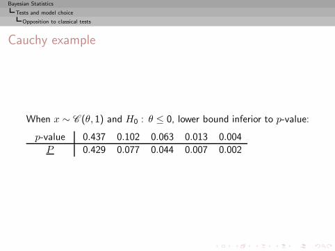
Bayesian Statistics
Tests and model choice
Opposition to classical tests
Cauchy example
When x ∼ C (θ, 1) and H0 : θ ≤ 0, lower bound inferior to p-value:
p-value 0.437 0.102 0.063 0.013 0.004
P 0.429 0.077 0.044 0.007 0.002
Bayesian Statistics
Tests and model choice
Model choice
Model choice and model comparison
Choice of models
Several models available for the same observation
Mi : x ∼ fi(x|θi), i ∈ I
where I can be finite or infinite
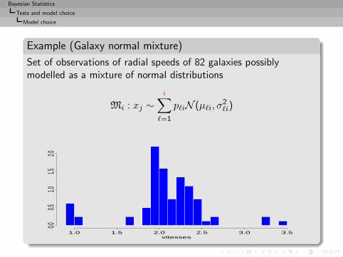
Bayesian Statistics
Tests and model choice
Model choice
Example (Galaxy normal mixture)
Set of observations of radial speeds of 82 galaxies possiblymodelled as a mixture of normal distributions
Mi : xj ∼i∑
ℓ=1
pℓiN (µℓi, σ2ℓi)
1.0 1.5 2.0 2.5 3.0 3.5
0.00.5
1.01.5
2.0
vitesses
Bayesian Statistics
Tests and model choice
Bayesian resolution
Bayesian resolution
B Framework
Probabilises the entire model/parameter space
Bayesian Statistics
Tests and model choice
Bayesian resolution
Bayesian resolution
B Framework
Probabilises the entire model/parameter spaceThis means:
◮ allocating probabilities pi to all models Mi
◮ defining priors πi(θi) for each parameter space Θi
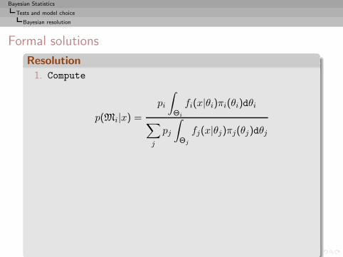
Bayesian Statistics
Tests and model choice
Bayesian resolution
Formal solutions
Resolution
1. Compute
p(Mi|x) =
pi
∫
Θi
fi(x|θi)πi(θi)dθi∑
j
pj
∫
Θj
fj(x|θj)πj(θj)dθj
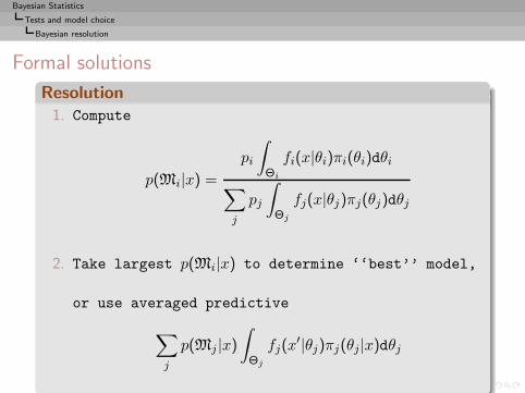
Bayesian Statistics
Tests and model choice
Bayesian resolution
Formal solutions
Resolution
1. Compute
p(Mi|x) =
pi
∫
Θi
fi(x|θi)πi(θi)dθi∑
j
pj
∫
Θj
fj(x|θj)πj(θj)dθj
2. Take largest p(Mi|x) to determine ‘‘best’’ model,
or use averaged predictive
∑
j
p(Mj |x)∫
Θj
fj(x′|θj)πj(θj|x)dθj
Bayesian Statistics
Tests and model choice
Problems
Several types of problems
◮ Concentrate on selection perspective:◮ averaging = estimation = non-parsimonious = no-decision◮ how to integrate loss function/decision/consequences
Bayesian Statistics
Tests and model choice
Problems
Several types of problems
◮ Concentrate on selection perspective:◮ averaging = estimation = non-parsimonious = no-decision◮ how to integrate loss function/decision/consequences◮ representation of parsimony/sparcity (Ockham’s rule)◮ how to fight overfitting for nested models
Which loss ?
Bayesian Statistics
Tests and model choice
Problems
Several types of problems (2)
◮ Choice of prior structures◮ adequate weights pi:
if M1 = M2 ∪ M3,
Bayesian Statistics
Tests and model choice
Problems
Several types of problems (2)
◮ Choice of prior structures◮ adequate weights pi:
if M1 = M2 ∪ M3, p(M1) = p(M2) + p(M3) ?◮ priors distributions
◮ πi(θi) defined for every i ∈ I
Bayesian Statistics
Tests and model choice
Problems
Several types of problems (2)
◮ Choice of prior structures◮ adequate weights pi:
if M1 = M2 ∪ M3, p(M1) = p(M2) + p(M3) ?◮ priors distributions
◮ πi(θi) defined for every i ∈ I
◮ πi(θi) proper (Jeffreys)
Bayesian Statistics
Tests and model choice
Problems
Several types of problems (2)
◮ Choice of prior structures◮ adequate weights pi:
if M1 = M2 ∪ M3, p(M1) = p(M2) + p(M3) ?◮ priors distributions
◮ πi(θi) defined for every i ∈ I
◮ πi(θi) proper (Jeffreys)◮ πi(θi) coherent (?) for nested models
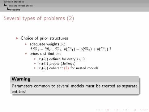
Bayesian Statistics
Tests and model choice
Problems
Several types of problems (2)
◮ Choice of prior structures◮ adequate weights pi:
if M1 = M2 ∪ M3, p(M1) = p(M2) + p(M3) ?◮ priors distributions
◮ πi(θi) defined for every i ∈ I
◮ πi(θi) proper (Jeffreys)◮ πi(θi) coherent (?) for nested models
Warning
Parameters common to several models must be treated as separateentities!

Bayesian Statistics
Tests and model choice
Problems
Several types of problems (3)
◮ Computation of predictives and marginals
- infinite dimensional spaces- integration over parameter spaces- integration over different spaces- summation over many models (2k)
Bayesian Statistics
Tests and model choice
Compatible priors
Compatibility principle
Difficulty of finding simultaneously priors on a collection of modelsMi (i ∈ I)

Bayesian Statistics
Tests and model choice
Compatible priors
Compatibility principle
Difficulty of finding simultaneously priors on a collection of modelsMi (i ∈ I)Easier to start from a single prior on a “big” model and to derivethe others from a coherence principle
[Dawid & Lauritzen, 2000]
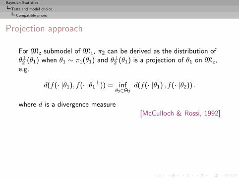
Bayesian Statistics
Tests and model choice
Compatible priors
Projection approach
For M2 submodel of M1, π2 can be derived as the distribution ofθ⊥2 (θ1) when θ1 ∼ π1(θ1) and θ⊥2 (θ1) is a projection of θ1 on M2,e.g.
d(f(· |θ1), f(· |θ1⊥)) = infθ2∈Θ2
d(f(· |θ1) , f(· |θ2)) .
where d is a divergence measure[McCulloch & Rossi, 1992]
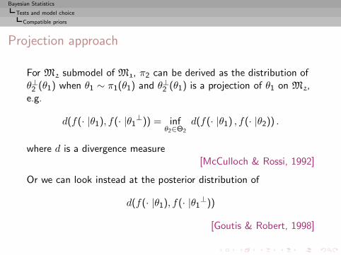
Or we can look instead at the posterior distribution of
d(f(· |θ1), f(· |θ1⊥))
[Goutis & Robert, 1998]
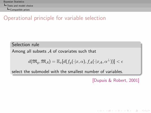
Bayesian Statistics
Tests and model choice
Compatible priors
Operational principle for variable selection
Selection rule
Among all subsets A of covariates such that
d(Mg,MA) = Ex[d(fg(·|x, α), fA(·|xA, α⊥))] < ǫ
select the submodel with the smallest number of variables.
[Dupuis & Robert, 2001]

Bayesian Statistics
Tests and model choice
Compatible priors
Kullback proximity
Alternative to above
Definition (Compatible prior)
Given a prior π1 on a model M1 and a submodel M2, a prior π2 onM2 is compatible with π1
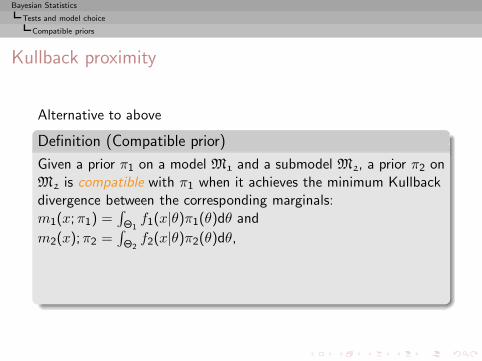
Bayesian Statistics
Tests and model choice
Compatible priors
Kullback proximity
Alternative to above
Definition (Compatible prior)
Given a prior π1 on a model M1 and a submodel M2, a prior π2 onM2 is compatible with π1 when it achieves the minimum Kullbackdivergence between the corresponding marginals:m1(x;π1) =
∫Θ1f1(x|θ)π1(θ)dθ and
m2(x);π2 =∫Θ2f2(x|θ)π2(θ)dθ,
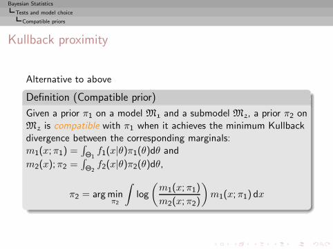
π2 = arg minπ2
∫log
(m1(x;π1)
m2(x;π2)
)m1(x;π1) dx

Bayesian Statistics
Tests and model choice
Compatible priors
Difficulties
◮ Does not give a working principle when M2 is not a submodelM1

Bayesian Statistics
Tests and model choice
Compatible priors
Difficulties
◮ Does not give a working principle when M2 is not a submodelM1
◮ Depends on the choice of π1
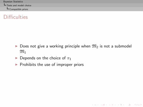
Bayesian Statistics
Tests and model choice
Compatible priors
Difficulties
◮ Does not give a working principle when M2 is not a submodelM1
◮ Depends on the choice of π1
◮ Prohibits the use of improper priors
Bayesian Statistics
Tests and model choice
Compatible priors
Difficulties
◮ Does not give a working principle when M2 is not a submodelM1
◮ Depends on the choice of π1
◮ Prohibits the use of improper priors
◮ Worse: useless in unconstrained settings...
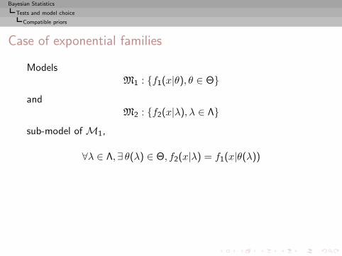
Bayesian Statistics
Tests and model choice
Compatible priors
Case of exponential families
ModelsM1 : {f1(x|θ), θ ∈ Θ}
andM2 : {f2(x|λ), λ ∈ Λ}
sub-model of M1,
∀λ ∈ Λ,∃ θ(λ) ∈ Θ, f2(x|λ) = f1(x|θ(λ))
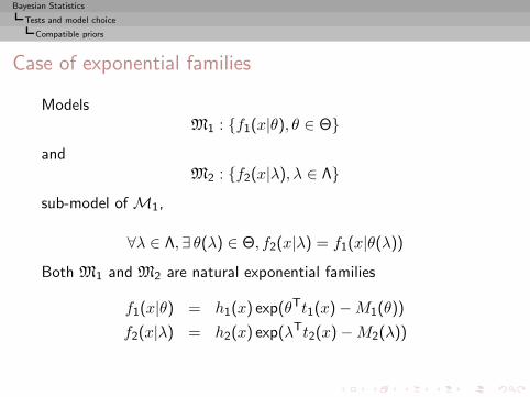
Bayesian Statistics
Tests and model choice
Compatible priors
Case of exponential families
ModelsM1 : {f1(x|θ), θ ∈ Θ}
andM2 : {f2(x|λ), λ ∈ Λ}
sub-model of M1,
∀λ ∈ Λ,∃ θ(λ) ∈ Θ, f2(x|λ) = f1(x|θ(λ))
Both M1 and M2 are natural exponential families
f1(x|θ) = h1(x) exp(θTt1(x) −M1(θ))
f2(x|λ) = h2(x) exp(λTt2(x) −M2(λ))
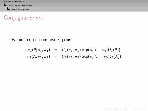
Bayesian Statistics
Tests and model choice
Compatible priors
Conjugate priors
Parameterised (conjugate) priors
π1(θ; s1, n1) = C1(s1, n1) exp(sT1 θ − n1M1(θ))
π2(λ; s2, n2) = C2(s2, n2) exp(sT2 λ− n2M2(λ))
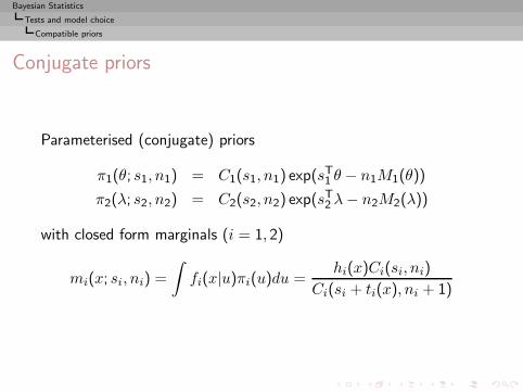
Bayesian Statistics
Tests and model choice
Compatible priors
Conjugate priors
Parameterised (conjugate) priors
π1(θ; s1, n1) = C1(s1, n1) exp(sT1 θ − n1M1(θ))
π2(λ; s2, n2) = C2(s2, n2) exp(sT2 λ− n2M2(λ))
with closed form marginals (i = 1, 2)
mi(x; si, ni) =
∫fi(x|u)πi(u)du =
hi(x)Ci(si, ni)
Ci(si + ti(x), ni + 1)
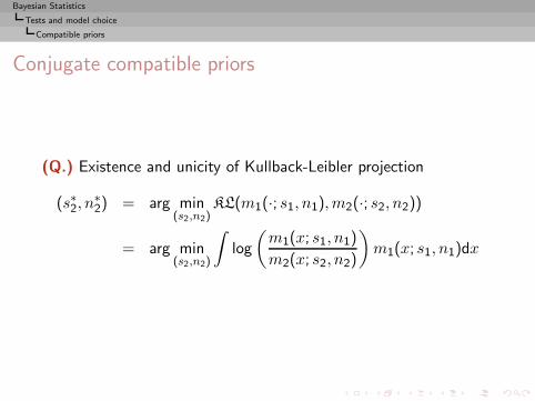
Bayesian Statistics
Tests and model choice
Compatible priors
Conjugate compatible priors
(Q.) Existence and unicity of Kullback-Leibler projection
(s∗2, n∗2) = arg min
(s2,n2)KL(m1(·; s1, n1),m2(·; s2, n2))
= arg min(s2,n2)
∫log
(m1(x; s1, n1)
m2(x; s2, n2)
)m1(x; s1, n1)dx
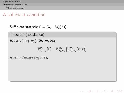
Bayesian Statistics
Tests and model choice
Compatible priors
A sufficient condition
Sufficient statistic ψ = (λ,−M2(λ))
Theorem (Existence)
If, for all (s2, n2), the matrix
Vπ2s2,n2
[ψ] − Em1s1,n1
[Vπ2s2,n2
(ψ|x)]
is semi-definite negative,
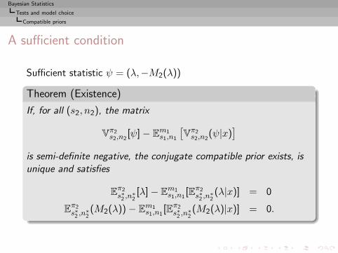
Bayesian Statistics
Tests and model choice
Compatible priors
A sufficient condition
Sufficient statistic ψ = (λ,−M2(λ))
Theorem (Existence)
If, for all (s2, n2), the matrix
Vπ2s2,n2
[ψ] − Em1s1,n1
[Vπ2s2,n2
(ψ|x)]
is semi-definite negative, the conjugate compatible prior exists, isunique and satisfies
Eπ2s∗2 ,n
∗2[λ] − E
m1s1,n1
[Eπ2s∗2 ,n
∗2(λ|x)] = 0
Eπ2s∗2 ,n
∗2(M2(λ)) − E
m1s1,n1
[Eπ2s∗2 ,n
∗2(M2(λ)|x)] = 0.
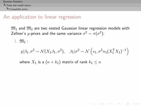
Bayesian Statistics
Tests and model choice
Compatible priors
An application to linear regression
M1 and M2 are two nested Gaussian linear regression models withZellner’s g-priors and the same variance σ2 ∼ π(σ2):
1. M1 :
y|β1, σ2 ∼ N (X1β1, σ
2), β1|σ2 ∼ N(s1, σ
2n1(XT1 X1)
−1)
where X1 is a (n× k1) matrix of rank k1 ≤ n
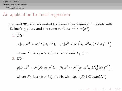
2. M2 :
y|β2, σ2 ∼ N (X2β2, σ
2), β2|σ2 ∼ N(s2, σ
2n2(XT2 X2)
−1),
where X2 is a (n× k2) matrix with span(X2) ⊆ span(X1)
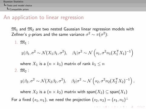
For a fixed (s1, n1), we need the projection (s2, n2) = (s1, n1)⊥

Bayesian Statistics
Tests and model choice
Compatible priors
Compatible g-priors
Since σ2 is a nuisance parameter, we can minimize theKullback-Leibler divergence between the two marginal distributionsconditional on σ2: m1(y|σ2; s1, n1) and m2(y|σ2; s2, n2)
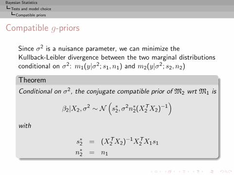
Bayesian Statistics
Tests and model choice
Compatible priors
Compatible g-priors
Since σ2 is a nuisance parameter, we can minimize theKullback-Leibler divergence between the two marginal distributionsconditional on σ2: m1(y|σ2; s1, n1) and m2(y|σ2; s2, n2)
Theorem
Conditional on σ2, the conjugate compatible prior of M2 wrt M1 is
β2|X2, σ2 ∼ N
(s∗2, σ
2n∗2(XT
2 X2)−1)
with
s∗2 = (XT
2 X2)−1XT
2 X1s1
n∗2 = n1
Bayesian Statistics
Tests and model choice
Variable selection
Variable selection
Regression setup where y regressed on a set {x1, . . . , xp} of ppotential explanatory regressors (plus intercept)
Bayesian Statistics
Tests and model choice
Variable selection
Variable selection
Regression setup where y regressed on a set {x1, . . . , xp} of ppotential explanatory regressors (plus intercept)
Corresponding 2p submodels Mγ , where γ ∈ Γ = {0, 1}p indicatesinclusion/exclusion of variables by a binary representation,
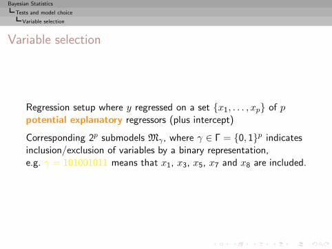
Bayesian Statistics
Tests and model choice
Variable selection
Variable selection
Regression setup where y regressed on a set {x1, . . . , xp} of ppotential explanatory regressors (plus intercept)
Corresponding 2p submodels Mγ , where γ ∈ Γ = {0, 1}p indicatesinclusion/exclusion of variables by a binary representation,e.g. γ = 101001011 means that x1, x3, x5, x7 and x8 are included.
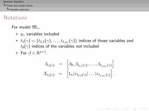
Bayesian Statistics
Tests and model choice
Variable selection
Notations
For model Mγ ,
◮ qγ variables included
◮ t1(γ) = {t1,1(γ), . . . , t1,qγ (γ)} indices of those variables andt0(γ) indices of the variables not included
◮ For β ∈ Rp+1,
βt1(γ) =[β0, βt1,1(γ), . . . , βt1,qγ (γ)
]
Xt1(γ) =[1n|xt1,1(γ)| . . . |xt1,qγ (γ)
].
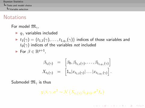
Submodel Mγ is thus
y|β, γ, σ2 ∼ N(Xt1(γ)βt1(γ), σ
2In)
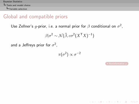
Bayesian Statistics
Tests and model choice
Variable selection
Global and compatible priors
Use Zellner’s g-prior, i.e. a normal prior for β conditional on σ2,
β|σ2 ∼ N (β, cσ2(XTX)−1)
and a Jeffreys prior for σ2,
π(σ2) ∝ σ−2
Noninformative g

Bayesian Statistics
Tests and model choice
Variable selection
Global and compatible priors
Use Zellner’s g-prior, i.e. a normal prior for β conditional on σ2,
β|σ2 ∼ N (β, cσ2(XTX)−1)
and a Jeffreys prior for σ2,
π(σ2) ∝ σ−2
Noninformative g
Resulting compatible prior
N((
XTt1(γ)
Xt1(γ)
)−1XTt1(γ)
Xβ, cσ2(XTt1(γ)
Xt1(γ)
)−1)
[Surprise!]

Bayesian Statistics
Tests and model choice
Variable selection
Global and compatible priors
Use Zellner’s g-prior, i.e. a normal prior for β conditional on σ2,
β|σ2 ∼ N (β, cσ2(XTX)−1)
and a Jeffreys prior for σ2,
π(σ2) ∝ σ−2
Noninformative g
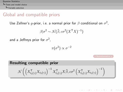
Bayesian Statistics
Tests and model choice
Variable selection
Global and compatible priors
Use Zellner’s g-prior, i.e. a normal prior for β conditional on σ2,
β|σ2 ∼ N (β, cσ2(XTX)−1)
and a Jeffreys prior for σ2,
π(σ2) ∝ σ−2
Noninformative g
Resulting compatible prior
N((
XTt1(γ)
Xt1(γ)
)−1XTt1(γ)
Xβ, cσ2(XTt1(γ)
Xt1(γ)
)−1)
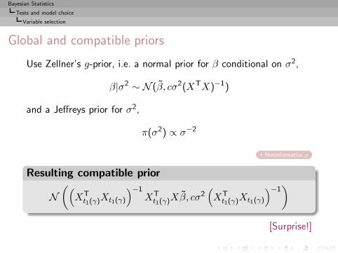
[Surprise!]
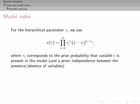
Bayesian Statistics
Tests and model choice
Variable selection
Model index
For the hierarchical parameter γ, we use
π(γ) =
p∏
i=1
τγi
i (1 − τi)1−γi ,
where τi corresponds to the prior probability that variable i ispresent in the model (and a priori independence between thepresence/absence of variables)
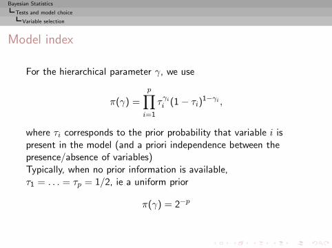
Bayesian Statistics
Tests and model choice
Variable selection
Model index
For the hierarchical parameter γ, we use
π(γ) =
p∏
i=1
τγi
i (1 − τi)1−γi ,
where τi corresponds to the prior probability that variable i ispresent in the model (and a priori independence between thepresence/absence of variables)Typically, when no prior information is available,τ1 = . . . = τp = 1/2, ie a uniform prior
π(γ) = 2−p
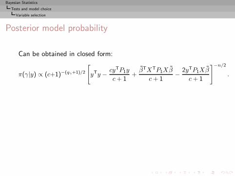
Bayesian Statistics
Tests and model choice
Variable selection
Posterior model probability
Can be obtained in closed form:
π(γ|y) ∝ (c+1)−(qγ+1)/2
[yTy − cyTP1y
c+ 1+βTXTP1Xβ
c+ 1− 2yTP1Xβ
c+ 1
]−n/2
.
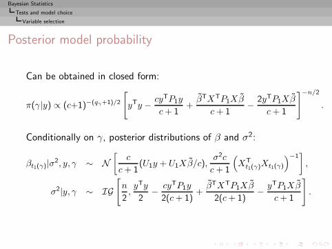
Bayesian Statistics
Tests and model choice
Variable selection
Posterior model probability
Can be obtained in closed form:
π(γ|y) ∝ (c+1)−(qγ+1)/2
[yTy − cyTP1y
c+ 1+βTXTP1Xβ
c+ 1− 2yTP1Xβ
c+ 1
]−n/2
.
Conditionally on γ, posterior distributions of β and σ2:
βt1(γ)|σ2, y, γ ∼ N[
c
c+ 1(U1y + U1Xβ/c),
σ2c
c+ 1
(XT
t1(γ)Xt1(γ)
)−1],
σ2|y, γ ∼ IG[n
2,yTy
2− cyTP1y
2(c+ 1)+βTXTP1Xβ
2(c+ 1)− yTP1Xβ
c+ 1
].
Bayesian Statistics
Tests and model choice
Variable selection
Noninformative case
Use the same compatible informative g-prior distribution withβ = 0p+1 and a hierarchical diffuse prior distribution on c,
π(c) ∝ c−1IN∗(c)
Recall g-prior
Bayesian Statistics
Tests and model choice
Variable selection
Noninformative case
Use the same compatible informative g-prior distribution withβ = 0p+1 and a hierarchical diffuse prior distribution on c,
π(c) ∝ c−1IN∗(c)
Recall g-prior
The choice of this hierarchical diffuse prior distribution on c is dueto the model posterior sensitivity to large values of c:
Taking β = 0p+1 and c large does not work
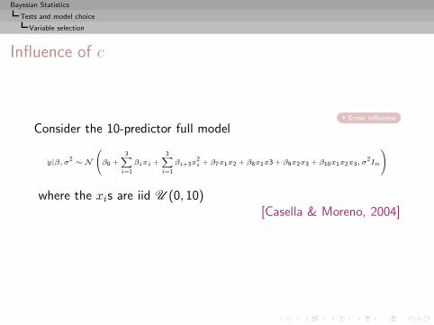
Bayesian Statistics
Tests and model choice
Variable selection
Influence of c
Erase influence
Consider the 10-predictor full model
y|β, σ2 ∼ N
0
@β0 +3
X
i=1
βixi +3
X
i=1
βi+3x2i + β7x1x2 + β8x1x3 + β9x2x3 + β10x1x2x3, σ
2In
1
A
where the xis are iid U (0, 10)[Casella & Moreno, 2004]
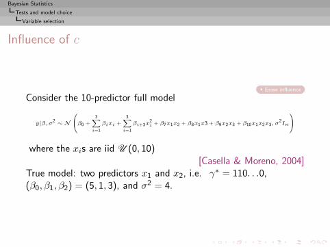
Bayesian Statistics
Tests and model choice
Variable selection
Influence of c
Erase influence
Consider the 10-predictor full model
y|β, σ2 ∼ N
0
@β0 +3
X
i=1
βixi +3
X
i=1
βi+3x2i + β7x1x2 + β8x1x3 + β9x2x3 + β10x1x2x3, σ
2In
1
A
where the xis are iid U (0, 10)[Casella & Moreno, 2004]
True model: two predictors x1 and x2, i.e. γ∗ = 110. . .0,(β0, β1, β2) = (5, 1, 3), and σ2 = 4.
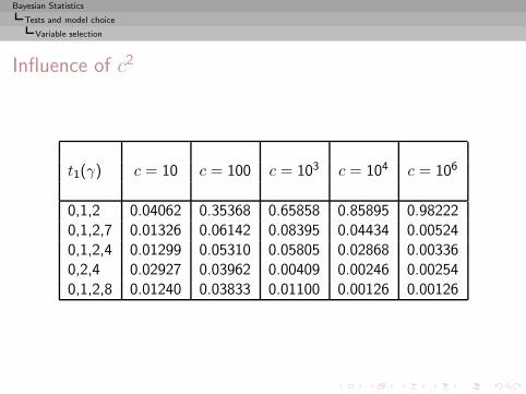
Bayesian Statistics
Tests and model choice
Variable selection
Influence of c2
t1(γ) c = 10 c = 100 c = 103 c = 104 c = 106
0,1,2 0.04062 0.35368 0.65858 0.85895 0.982220,1,2,7 0.01326 0.06142 0.08395 0.04434 0.005240,1,2,4 0.01299 0.05310 0.05805 0.02868 0.003360,2,4 0.02927 0.03962 0.00409 0.00246 0.002540,1,2,8 0.01240 0.03833 0.01100 0.00126 0.00126
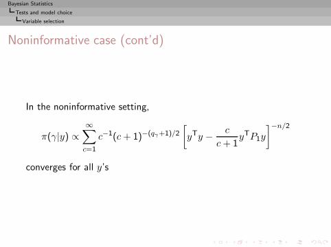
Bayesian Statistics
Tests and model choice
Variable selection
Noninformative case (cont’d)
In the noninformative setting,
π(γ|y) ∝∞∑
c=1
c−1(c+ 1)−(qγ+1)/2
[yTy − c
c+ 1yTP1y
]−n/2
converges for all y’s
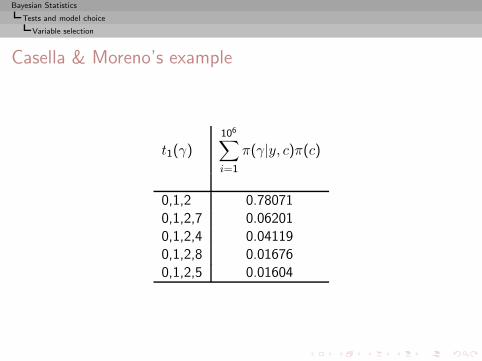
Bayesian Statistics
Tests and model choice
Variable selection
Casella & Moreno’s example
t1(γ)106∑
i=1
π(γ|y, c)π(c)
0,1,2 0.780710,1,2,7 0.062010,1,2,4 0.041190,1,2,8 0.016760,1,2,5 0.01604

Bayesian Statistics
Tests and model choice
Variable selection
Gibbs approximation
When p large, impossible to compute the posterior probabilities ofthe 2p models.
Bayesian Statistics
Tests and model choice
Variable selection
Gibbs approximation
When p large, impossible to compute the posterior probabilities ofthe 2p models.Use of a Monte Carlo approximation of π(γ|y)
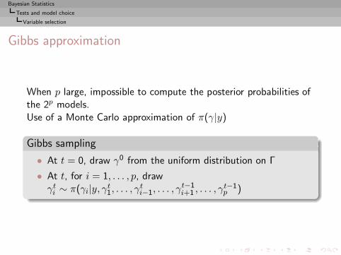
Bayesian Statistics
Tests and model choice
Variable selection
Gibbs approximation
When p large, impossible to compute the posterior probabilities ofthe 2p models.Use of a Monte Carlo approximation of π(γ|y)
Gibbs sampling
• At t = 0, draw γ0 from the uniform distribution on Γ
• At t, for i = 1, . . . , p, drawγti ∼ π(γi|y, γt1, . . . , γti−1, . . . , γ
t−1i+1 , . . . , γ
t−1p )
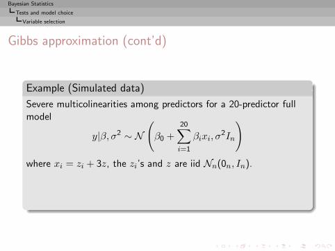
Bayesian Statistics
Tests and model choice
Variable selection
Gibbs approximation (cont’d)
Example (Simulated data)
Severe multicolinearities among predictors for a 20-predictor fullmodel
y|β, σ2 ∼ N(
β0 +
20∑
i=1
βixi, σ2In
)
where xi = zi + 3z, the zi’s and z are iid Nn(0n, In).
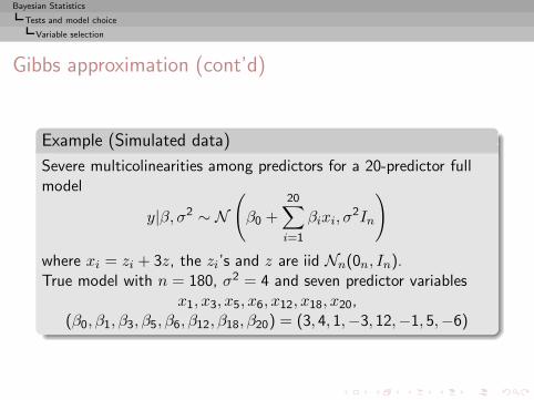
Bayesian Statistics
Tests and model choice
Variable selection
Gibbs approximation (cont’d)
Example (Simulated data)
Severe multicolinearities among predictors for a 20-predictor fullmodel
y|β, σ2 ∼ N(
β0 +
20∑
i=1
βixi, σ2In
)
where xi = zi + 3z, the zi’s and z are iid Nn(0n, In).True model with n = 180, σ2 = 4 and seven predictor variables
x1, x3, x5, x6, x12, x18, x20,(β0, β1, β3, β5, β6, β12, β18, β20) = (3, 4, 1,−3, 12,−1, 5,−6)
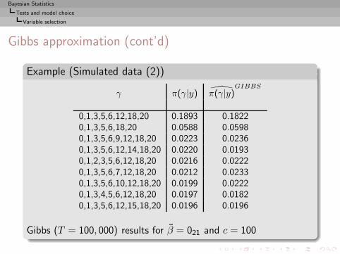
Bayesian Statistics
Tests and model choice
Variable selection
Gibbs approximation (cont’d)
Example (Simulated data (2))
γ π(γ|y) π(γ|y)GIBBS
0,1,3,5,6,12,18,20 0.1893 0.18220,1,3,5,6,18,20 0.0588 0.05980,1,3,5,6,9,12,18,20 0.0223 0.02360,1,3,5,6,12,14,18,20 0.0220 0.01930,1,2,3,5,6,12,18,20 0.0216 0.02220,1,3,5,6,7,12,18,20 0.0212 0.02330,1,3,5,6,10,12,18,20 0.0199 0.02220,1,3,4,5,6,12,18,20 0.0197 0.01820,1,3,5,6,12,15,18,20 0.0196 0.0196
Gibbs (T = 100, 000) results for β = 021 and c = 100

Bayesian Statistics
Tests and model choice
Variable selection
Processionary caterpillar
Influence of some forest settlement characteristics on thedevelopment of caterpillar colonies

Bayesian Statistics
Tests and model choice
Variable selection
Processionary caterpillar
Influence of some forest settlement characteristics on thedevelopment of caterpillar colonies

Bayesian Statistics
Tests and model choice
Variable selection
Processionary caterpillar
Influence of some forest settlement characteristics on thedevelopment of caterpillar colonies
Response y log-transform of the average number of nests ofcaterpillars per tree on an area of 500 square meters (n = 33 areas)
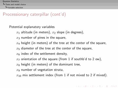
Bayesian Statistics
Tests and model choice
Variable selection
Processionary caterpillar (cont’d)
Potential explanatory variables
x1 altitude (in meters), x2 slope (in degrees),
x3 number of pines in the square,
x4 height (in meters) of the tree at the center of the square,
x5 diameter of the tree at the center of the square,
x6 index of the settlement density,
x7 orientation of the square (from 1 if southb’d to 2 ow),
x8 height (in meters) of the dominant tree,
x9 number of vegetation strata,
x10 mix settlement index (from 1 if not mixed to 2 if mixed).
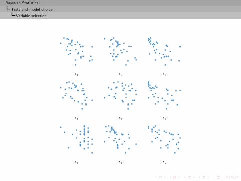
Bayesian Statistics
Tests and model choice
Variable selection
x1 x2 x3
x4 x5 x6
x7 x8 x9
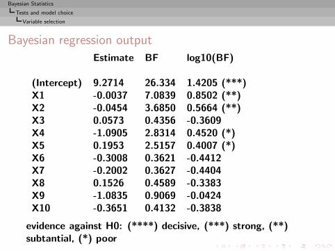
Bayesian Statistics
Tests and model choice
Variable selection
Bayesian regression output
Estimate BF log10(BF)
(Intercept) 9.2714 26.334 1.4205 (***)X1 -0.0037 7.0839 0.8502 (**)X2 -0.0454 3.6850 0.5664 (**)X3 0.0573 0.4356 -0.3609X4 -1.0905 2.8314 0.4520 (*)X5 0.1953 2.5157 0.4007 (*)X6 -0.3008 0.3621 -0.4412X7 -0.2002 0.3627 -0.4404X8 0.1526 0.4589 -0.3383X9 -1.0835 0.9069 -0.0424X10 -0.3651 0.4132 -0.3838
evidence against H0: (****) decisive, (***) strong, (**)subtantial, (*) poor
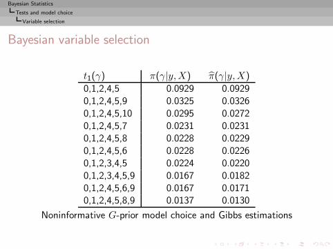
Bayesian Statistics
Tests and model choice
Variable selection
Bayesian variable selection
t1(γ) π(γ|y,X) π(γ|y,X)
0,1,2,4,5 0.0929 0.09290,1,2,4,5,9 0.0325 0.03260,1,2,4,5,10 0.0295 0.02720,1,2,4,5,7 0.0231 0.02310,1,2,4,5,8 0.0228 0.02290,1,2,4,5,6 0.0228 0.02260,1,2,3,4,5 0.0224 0.02200,1,2,3,4,5,9 0.0167 0.01820,1,2,4,5,6,9 0.0167 0.01710,1,2,4,5,8,9 0.0137 0.0130
Noninformative G-prior model choice and Gibbs estimations

Bayesian Statistics
Tests and model choice
Symmetrised compatible priors
Postulate
Previous principle requires embedded models (or an encompassingmodel) and proper priors, while being hard to implement outsideexponential families
Bayesian Statistics
Tests and model choice
Symmetrised compatible priors
Postulate
Previous principle requires embedded models (or an encompassingmodel) and proper priors, while being hard to implement outsideexponential familiesNow we determine prior measures on two models M1 and M2, π1
and π2, directly by a compatibility principle.
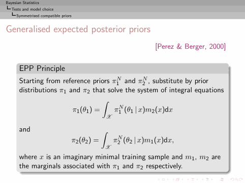
Bayesian Statistics
Tests and model choice
Symmetrised compatible priors
Generalised expected posterior priors
[Perez & Berger, 2000]
EPP Principle
Starting from reference priors πN1 and πN2 , substitute by priordistributions π1 and π2 that solve the system of integral equations
π1(θ1) =
∫
X
πN1 (θ1 |x)m2(x)dx
and
π2(θ2) =
∫
X
πN2 (θ2 |x)m1(x)dx,
where x is an imaginary minimal training sample and m1, m2 arethe marginals associated with π1 and π2 respectively.

Bayesian Statistics
Tests and model choice
Symmetrised compatible priors
Motivations
◮ Eliminates the “imaginary observation” device andproper-isation through part of the data by integration underthe “truth”
Bayesian Statistics
Tests and model choice
Symmetrised compatible priors
Motivations
◮ Eliminates the “imaginary observation” device andproper-isation through part of the data by integration underthe “truth”
◮ Assumes that both models are equally valid and equippedwith ideal unknown priors
πi, i = 1, 2,
that yield “true” marginals balancing each model wrt theother
◮ For a given π1, π2 is an expected posterior priorUsing both equations introduces symmetry into the game
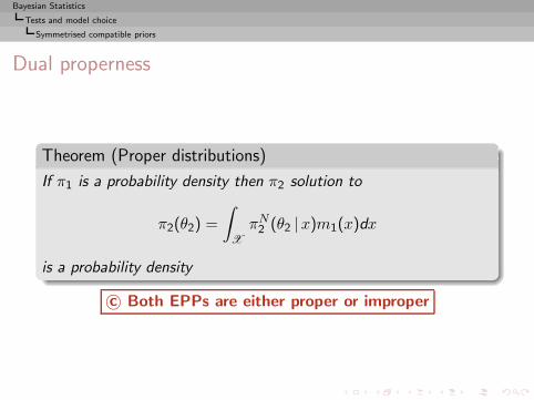
Bayesian Statistics
Tests and model choice
Symmetrised compatible priors
Dual properness
Theorem (Proper distributions)
If π1 is a probability density then π2 solution to
π2(θ2) =
∫
X
πN2 (θ2 |x)m1(x)dx
is a probability density
c© Both EPPs are either proper or improper
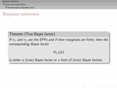
Bayesian Statistics
Tests and model choice
Symmetrised compatible priors
Bayesian coherence
Theorem (True Bayes factor)
If π1 and π2 are the EPPs and if their marginals are finite, then thecorresponding Bayes factor
B1,2(x)
is either a (true) Bayes factor or a limit of (true) Bayes factors.
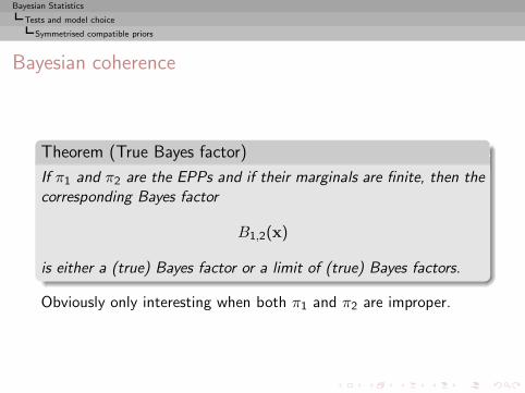
Bayesian Statistics
Tests and model choice
Symmetrised compatible priors
Bayesian coherence
Theorem (True Bayes factor)
If π1 and π2 are the EPPs and if their marginals are finite, then thecorresponding Bayes factor
B1,2(x)
is either a (true) Bayes factor or a limit of (true) Bayes factors.
Obviously only interesting when both π1 and π2 are improper.
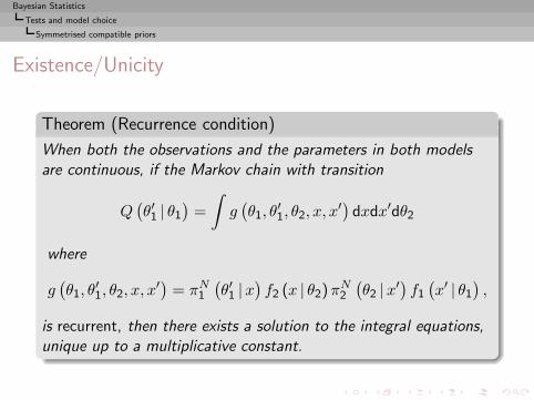
Bayesian Statistics
Tests and model choice
Symmetrised compatible priors
Existence/Unicity
Theorem (Recurrence condition)
When both the observations and the parameters in both modelsare continuous, if the Markov chain with transition
Q(θ′1 | θ1
)=
∫g(θ1, θ
′1, θ2, x, x
′) dxdx′dθ2
where
g(θ1, θ
′1, θ2, x, x
′) = πN1(θ′1 |x
)f2 (x | θ2)πN2
(θ2 |x′
)f1
(x′ | θ1
),
is recurrent, then there exists a solution to the integral equations,unique up to a multiplicative constant.
Bayesian Statistics
Tests and model choice
Symmetrised compatible priors
Consequences
◮ If the M chain is positive recurrent, there exists a unique pairof proper EPPS.
Bayesian Statistics
Tests and model choice
Symmetrised compatible priors
Consequences
◮ If the M chain is positive recurrent, there exists a unique pairof proper EPPS.
◮ The transition density Q (θ′1 | θ1) has a dual transition densityon Θ2.
Bayesian Statistics
Tests and model choice
Symmetrised compatible priors
Consequences
◮ If the M chain is positive recurrent, there exists a unique pairof proper EPPS.
◮ The transition density Q (θ′1 | θ1) has a dual transition densityon Θ2.
◮ There exists a parallel M chain on Θ2 with identicalproperties; if one is (Harris) recurrent, so is the other.
◮ Duality property found both in the MCMC literature and indecision theory
[Diebolt & Robert, 1992; Eaton, 1992]
◮ When Harris recurrence holds but the EPPs cannot be found,the Bayes factor can be approximated by MCMC simulation
Bayesian Statistics
Tests and model choice
Examples
Point null hypothesis testing
Testing H0 : θ = θ∗ versus H1 : θ 6= θ∗, i.e.
M1 : f (x | θ∗) ,M2 : f (x | θ) , θ ∈ Θ.
Bayesian Statistics
Tests and model choice
Examples
Point null hypothesis testing
Testing H0 : θ = θ∗ versus H1 : θ 6= θ∗, i.e.
M1 : f (x | θ∗) ,M2 : f (x | θ) , θ ∈ Θ.
Default priors
πN1 (θ) = δθ∗ (θ) and πN2 (θ) = πN (θ)
Bayesian Statistics
Tests and model choice
Examples
Point null hypothesis testing
Testing H0 : θ = θ∗ versus H1 : θ 6= θ∗, i.e.
M1 : f (x | θ∗) ,M2 : f (x | θ) , θ ∈ Θ.
Default priors
πN1 (θ) = δθ∗ (θ) and πN2 (θ) = πN (θ)
For x minimal training sample, consider the proper priors
π1 (θ) = δθ∗ (θ) and π2 (θ) =
∫πN (θ |x) f (x | θ∗) dx
Bayesian Statistics
Tests and model choice
Examples
Point null hypothesis testing (cont’d)
Then∫πN1 (θ |x)m2 (x) dx = δθ∗ (θ)
∫m2 (x) dx = δθ∗ (θ) = π1 (θ)
and∫πN2 (θ |x)m1 (x) dx =
∫πN (θ |x) f (x | θ∗) dx = π2 (θ)
Bayesian Statistics
Tests and model choice
Examples
Point null hypothesis testing (cont’d)
Then∫πN1 (θ |x)m2 (x) dx = δθ∗ (θ)
∫m2 (x) dx = δθ∗ (θ) = π1 (θ)
and∫πN2 (θ |x)m1 (x) dx =
∫πN (θ |x) f (x | θ∗) dx = π2 (θ)
c©π1 (θ) and π2 (θ) are integral priors
Bayesian Statistics
Tests and model choice
Examples
Point null hypothesis testing (cont’d)
Then∫πN1 (θ |x)m2 (x) dx = δθ∗ (θ)
∫m2 (x) dx = δθ∗ (θ) = π1 (θ)
and∫πN2 (θ |x)m1 (x) dx =
∫πN (θ |x) f (x | θ∗) dx = π2 (θ)
c©π1 (θ) and π2 (θ) are integral priors
Note
Uniqueness of the Bayes factorIntegral priors and intrinsic priors coincide
[Moreno, Bertolino and Racugno, 1998]
Bayesian Statistics
Tests and model choice
Examples
Location models
Two location models
M1 : f1 (x | θ1) = f1 (x− θ1)
M2 : f2 (x | θ2) = f2 (x− θ2)
Bayesian Statistics
Tests and model choice
Examples
Location models
Two location models
M1 : f1 (x | θ1) = f1 (x− θ1)
M2 : f2 (x | θ2) = f2 (x− θ2)
Default priorsπNi (θi) = ci, i = 1, 2
with minimal training sample size one
Bayesian Statistics
Tests and model choice
Examples
Location models
Two location models
M1 : f1 (x | θ1) = f1 (x− θ1)
M2 : f2 (x | θ2) = f2 (x− θ2)
Default priorsπNi (θi) = ci, i = 1, 2
with minimal training sample size oneMarginal densities
mNi (x) = ci, i = 1, 2
Bayesian Statistics
Tests and model choice
Examples
Location models (cont’d)
In that case, πN1 (θ1) and πN2 (θ2) are integral priors when c1 = c2:
∫πN1 (θ1 |x)mN
2 (x) dx =
∫c2f1 (x− θ1) dx = c2
∫πN2 (θ2 |x)mN
1 (x) dx =
∫c1f2 (x− θ2) dx = c1.
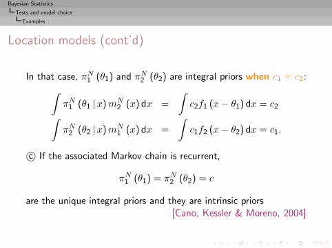
Bayesian Statistics
Tests and model choice
Examples
Location models (cont’d)
In that case, πN1 (θ1) and πN2 (θ2) are integral priors when c1 = c2:
∫πN1 (θ1 |x)mN
2 (x) dx =
∫c2f1 (x− θ1) dx = c2
∫πN2 (θ2 |x)mN
1 (x) dx =
∫c1f2 (x− θ2) dx = c1.
c© If the associated Markov chain is recurrent,
πN1 (θ1) = πN2 (θ2) = c
are the unique integral priors and they are intrinsic priors[Cano, Kessler & Moreno, 2004]
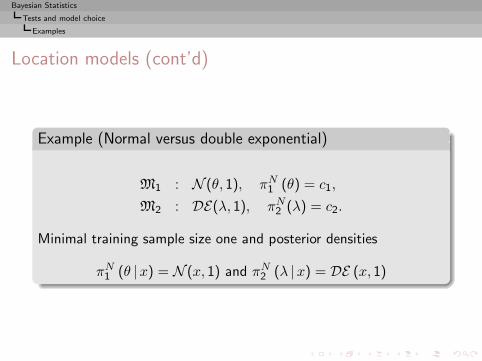
Bayesian Statistics
Tests and model choice
Examples
Location models (cont’d)
Example (Normal versus double exponential)
M1 : N (θ, 1), πN1 (θ) = c1,
M2 : DE(λ, 1), πN2 (λ) = c2.
Minimal training sample size one and posterior densities
πN1 (θ |x) = N (x, 1) and πN2 (λ |x) = DE (x, 1)
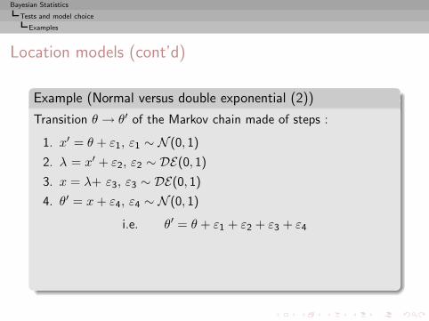
Bayesian Statistics
Tests and model choice
Examples
Location models (cont’d)
Example (Normal versus double exponential (2))
Transition θ → θ′ of the Markov chain made of steps :
1. x′ = θ + ε1, ε1 ∼ N (0, 1)
2. λ = x′ + ε2, ε2 ∼ DE(0, 1)
3. x = λ+ ε3, ε3 ∼ DE(0, 1)
4. θ′ = x+ ε4, ε4 ∼ N (0, 1)
i.e. θ′ = θ + ε1 + ε2 + ε3 + ε4
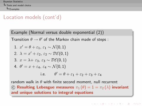
random walk in θ with finite second moment, null recurrentc© Resulting Lebesgue measures π1 (θ) = 1 = π2 (λ) invariantand unique solutions to integral equations

Bayesian Statistics
Admissibility and Complete Classes
Admissibility and Complete Classes
Introduction
Decision-Theoretic Foundations of Statistical Inference
From Prior Information to Prior Distributions
Bayesian Point Estimation
Bayesian Calculations
Tests and model choice
Admissibility and Complete ClassesAdmissibility of Bayes estimators
Bayesian Statistics
Admissibility and Complete Classes
Admissibility of Bayes estimators
Admissibility of Bayes estimators
Warning
Bayes estimators may be inadmissible when the Bayes risk is infinite
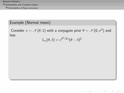
Bayesian Statistics
Admissibility and Complete Classes
Admissibility of Bayes estimators
Example (Normal mean)
Consider x ∼ N (θ, 1) with a conjugate prior θ ∼ N (0, σ2) andloss
Lα(θ, δ) = eθ2/2α(θ − δ)2
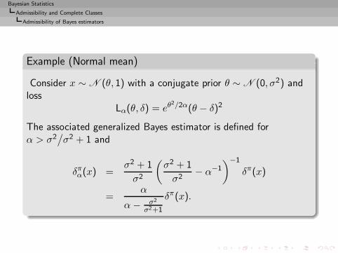
Bayesian Statistics
Admissibility and Complete Classes
Admissibility of Bayes estimators
Example (Normal mean)
Consider x ∼ N (θ, 1) with a conjugate prior θ ∼ N (0, σ2) andloss
Lα(θ, δ) = eθ2/2α(θ − δ)2
The associated generalized Bayes estimator is defined forα > σ2
/σ2 + 1 and
δπα(x) =σ2 + 1
σ2
(σ2 + 1
σ2− α−1
)−1
δπ(x)
=α
α− σ2
σ2+1
δπ(x).
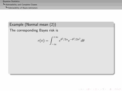
Bayesian Statistics
Admissibility and Complete Classes
Admissibility of Bayes estimators
Example (Normal mean (2))
The corresponding Bayes risk is
r(π) =
∫ +∞
−∞eθ
2/2αe−θ2/2σ2
dθ
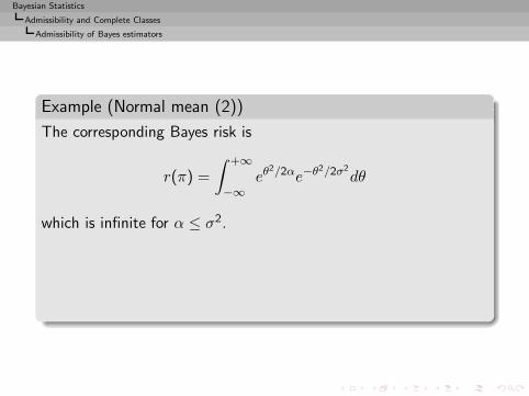
Bayesian Statistics
Admissibility and Complete Classes
Admissibility of Bayes estimators
Example (Normal mean (2))
The corresponding Bayes risk is
r(π) =
∫ +∞
−∞eθ
2/2αe−θ2/2σ2
dθ
which is infinite for α ≤ σ2.
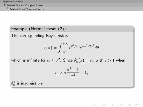
Bayesian Statistics
Admissibility and Complete Classes
Admissibility of Bayes estimators
Example (Normal mean (2))
The corresponding Bayes risk is
r(π) =
∫ +∞
−∞eθ
2/2αe−θ2/2σ2
dθ
which is infinite for α ≤ σ2. Since δπα(x) = cx with c > 1 when
α > ασ2 + 1
σ2− 1,
δπα is inadmissible
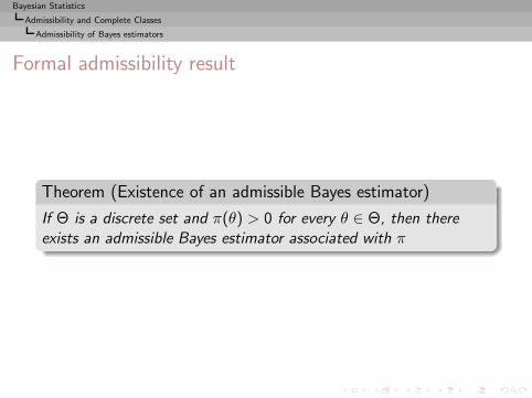
Bayesian Statistics
Admissibility and Complete Classes
Admissibility of Bayes estimators
Formal admissibility result
Theorem (Existence of an admissible Bayes estimator)
If Θ is a discrete set and π(θ) > 0 for every θ ∈ Θ, then thereexists an admissible Bayes estimator associated with π
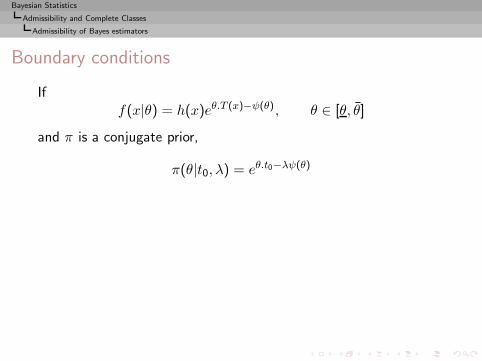
Bayesian Statistics
Admissibility and Complete Classes
Admissibility of Bayes estimators
Boundary conditions
Iff(x|θ) = h(x)eθ.T (x)−ψ(θ), θ ∈ [θ, θ]
and π is a conjugate prior,
π(θ|t0, λ) = eθ.t0−λψ(θ)
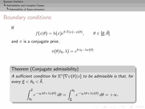
Bayesian Statistics
Admissibility and Complete Classes
Admissibility of Bayes estimators
Boundary conditions
Iff(x|θ) = h(x)eθ.T (x)−ψ(θ), θ ∈ [θ, θ]
and π is a conjugate prior,
π(θ|t0, λ) = eθ.t0−λψ(θ)
Theorem (Conjugate admissibility)
A sufficient condition for Eπ[∇ψ(θ)|x] to be admissible is that, forevery θ < θ0 < θ,
∫ θ
θ0
e−γ0λθ+λψ(θ) dθ =
∫ θ0
θe−γ0λθ+λψ(θ) dθ = +∞.
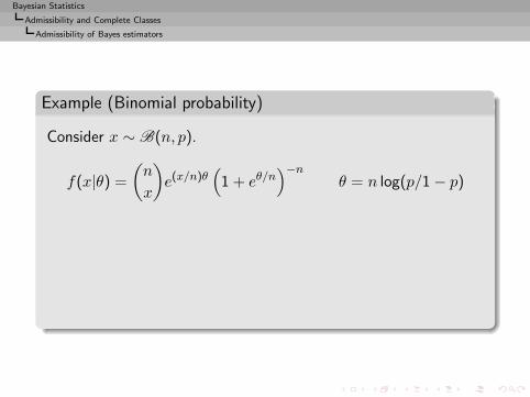
Bayesian Statistics
Admissibility and Complete Classes
Admissibility of Bayes estimators
Example (Binomial probability)
Consider x ∼ B(n, p).
f(x|θ) =
(n
x
)e(x/n)θ
(1 + eθ/n
)−nθ = n log(p/1 − p)
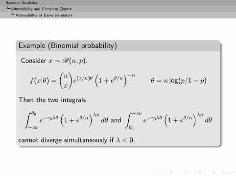
Bayesian Statistics
Admissibility and Complete Classes
Admissibility of Bayes estimators
Example (Binomial probability)
Consider x ∼ B(n, p).
f(x|θ) =
(n
x
)e(x/n)θ
(1 + eθ/n
)−nθ = n log(p/1 − p)
Then the two integrals
∫ θ0
−∞e−γ0λθ
(1 + eθ/n
)λndθ and
∫ +∞
θ0
e−γ0λθ(1 + eθ/n
)λndθ
cannot diverge simultaneously if λ < 0.
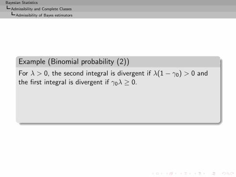
Bayesian Statistics
Admissibility and Complete Classes
Admissibility of Bayes estimators
Example (Binomial probability (2))
For λ > 0, the second integral is divergent if λ(1 − γ0) > 0 andthe first integral is divergent if γ0λ ≥ 0.
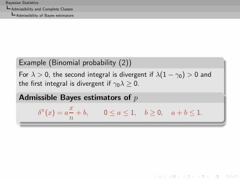
Bayesian Statistics
Admissibility and Complete Classes
Admissibility of Bayes estimators
Example (Binomial probability (2))
For λ > 0, the second integral is divergent if λ(1 − γ0) > 0 andthe first integral is divergent if γ0λ ≥ 0.
Admissible Bayes estimators of p
δπ(x) = ax
n+ b, 0 ≤ a ≤ 1, b ≥ 0, a+ b ≤ 1.
Bayesian Statistics
Admissibility and Complete Classes
Admissibility of Bayes estimators
Differential representations
Setting of multidimensional exponential families
f(x|θ) = h(x)eθ.x−ψ(θ), θ ∈ Rp
Bayesian Statistics
Admissibility and Complete Classes
Admissibility of Bayes estimators
Differential representations
Setting of multidimensional exponential families
f(x|θ) = h(x)eθ.x−ψ(θ), θ ∈ Rp
Measure g such that
Ix(∇g) =
∫||∇g(θ)||eθ.x−ψ(θ) dθ < +∞
Bayesian Statistics
Admissibility and Complete Classes
Admissibility of Bayes estimators
Differential representations
Setting of multidimensional exponential families
f(x|θ) = h(x)eθ.x−ψ(θ), θ ∈ Rp
Measure g such that
Ix(∇g) =
∫||∇g(θ)||eθ.x−ψ(θ) dθ < +∞
Representation of the posterior mean of ∇ψ(θ)
δg(x) = x+Ix(∇g)Ix(g)
.
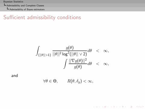
Bayesian Statistics
Admissibility and Complete Classes
Admissibility of Bayes estimators
Sufficient admissibility conditions
∫
{||θ||>1}
g(θ)
||θ||2 log2(||θ|| ∨ 2)dθ < ∞,
∫ ||∇g(θ)||2g(θ)
dθ < ∞,
and∀θ ∈ Θ, R(θ, δg) <∞,
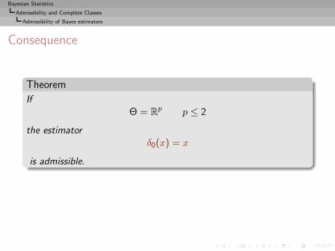
Bayesian Statistics
Admissibility and Complete Classes
Admissibility of Bayes estimators
Consequence
Theorem
IfΘ = R
p p ≤ 2
the estimatorδ0(x) = x
is admissible.
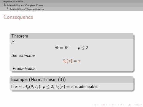
Bayesian Statistics
Admissibility and Complete Classes
Admissibility of Bayes estimators
Consequence
Theorem
IfΘ = R
p p ≤ 2
the estimatorδ0(x) = x
is admissible.
Example (Normal mean (3))
If x ∼ Np(θ, Ip), p ≤ 2, δ0(x) = x is admissible.
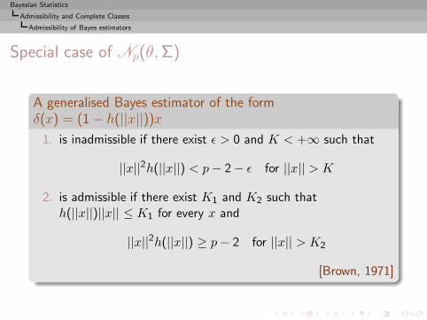
Bayesian Statistics
Admissibility and Complete Classes
Admissibility of Bayes estimators
Special case of Np(θ, Σ)
A generalised Bayes estimator of the formδ(x) = (1 − h(||x||))x
1. is inadmissible if there exist ǫ > 0 and K < +∞ such that
||x||2h(||x||) < p− 2 − ǫ for ||x|| > K
2. is admissible if there exist K1 and K2 such thath(||x||)||x|| ≤ K1 for every x and
||x||2h(||x||) ≥ p− 2 for ||x|| > K2
[Brown, 1971]
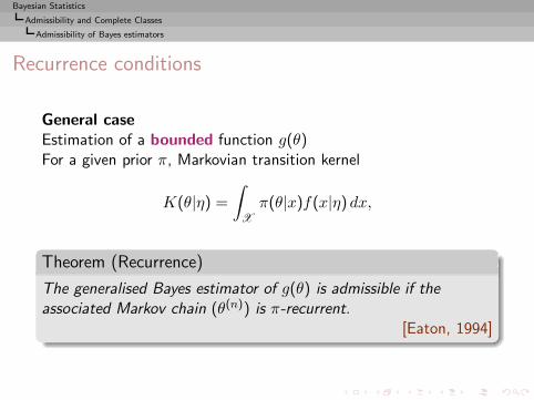
Bayesian Statistics
Admissibility and Complete Classes
Admissibility of Bayes estimators
Recurrence conditions
General caseEstimation of a bounded function g(θ)For a given prior π, Markovian transition kernel
K(θ|η) =
∫
X
π(θ|x)f(x|η) dx,
Theorem (Recurrence)
The generalised Bayes estimator of g(θ) is admissible if theassociated Markov chain (θ(n)) is π-recurrent.
[Eaton, 1994]
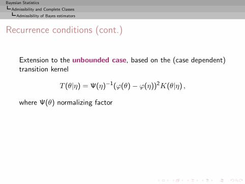
Bayesian Statistics
Admissibility and Complete Classes
Admissibility of Bayes estimators
Recurrence conditions (cont.)
Extension to the unbounded case, based on the (case dependent)transition kernel
T (θ|η) = Ψ(η)−1(ϕ(θ) − ϕ(η))2K(θ|η) ,
where Ψ(θ) normalizing factor
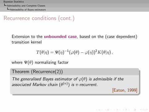
Bayesian Statistics
Admissibility and Complete Classes
Admissibility of Bayes estimators
Recurrence conditions (cont.)
Extension to the unbounded case, based on the (case dependent)transition kernel
T (θ|η) = Ψ(η)−1(ϕ(θ) − ϕ(η))2K(θ|η) ,
where Ψ(θ) normalizing factor
Theorem (Recurrence(2))
The generalised Bayes estimator of ϕ(θ) is admissible if theassociated Markov chain (θ(n)) is π-recurrent.
[Eaton, 1999]

Bayesian Statistics
Admissibility and Complete Classes
Necessary and sufficient admissibility conditions
Necessary and sufficient admissibility conditions
Formalisation of the statement that...

Bayesian Statistics
Admissibility and Complete Classes
Necessary and sufficient admissibility conditions
Necessary and sufficient admissibility conditions
Formalisation of the statement that......all admissible estimators are limits of Bayes estimators...
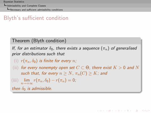
Bayesian Statistics
Admissibility and Complete Classes
Necessary and sufficient admissibility conditions
Blyth’s sufficient condition
Theorem (Blyth condition)
If, for an estimator δ0, there exists a sequence (πn) of generalisedprior distributions such that
(i) r(πn, δ0) is finite for every n;
(ii) for every nonempty open set C ⊂ Θ, there exist K > 0 and Nsuch that, for every n ≥ N , πn(C) ≥ K; and
(iii) limn→+∞
r(πn, δ0) − r(πn) = 0;
then δ0 is admissible.
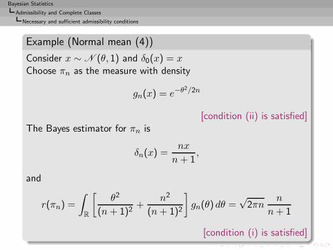
Bayesian Statistics
Admissibility and Complete Classes
Necessary and sufficient admissibility conditions
Example (Normal mean (4))
Consider x ∼ N (θ, 1) and δ0(x) = xChoose πn as the measure with density
gn(x) = e−θ2/2n
[condition (ii) is satisfied]The Bayes estimator for πn is
δn(x) =nx
n+ 1,
and
r(πn) =
∫
R
[θ2
(n+ 1)2+
n2
(n+ 1)2
]gn(θ) dθ =
√2πn
n
n+ 1
[condition (i) is satisfied]
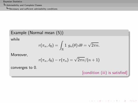
Bayesian Statistics
Admissibility and Complete Classes
Necessary and sufficient admissibility conditions
Example (Normal mean (5))
while
r(πn, δ0) =
∫
R
1 gn(θ) dθ =√
2πn.
Moreover,r(πn, δ0) − r(πn) =
√2πn/(n+ 1)
converges to 0.[condition (iii) is satisfied]
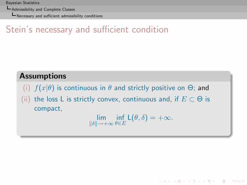
Bayesian Statistics
Admissibility and Complete Classes
Necessary and sufficient admissibility conditions
Stein’s necessary and sufficient condition
Assumptions
(i) f(x|θ) is continuous in θ and strictly positive on Θ; and
(ii) the loss L is strictly convex, continuous and, if E ⊂ Θ iscompact,
lim‖δ‖→+∞
infθ∈E
L(θ, δ) = +∞.
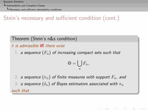
Bayesian Statistics
Admissibility and Complete Classes
Necessary and sufficient admissibility conditions
Stein’s necessary and sufficient condition (cont.)
Theorem (Stein’s n&s condition)
δ is admissible iff there exist
1. a sequence (Fn) of increasing compact sets such that
Θ =⋃
n
Fn,
2. a sequence (πn) of finite measures with support Fn, and
3. a sequence (δn) of Bayes estimators associated with πn
such that
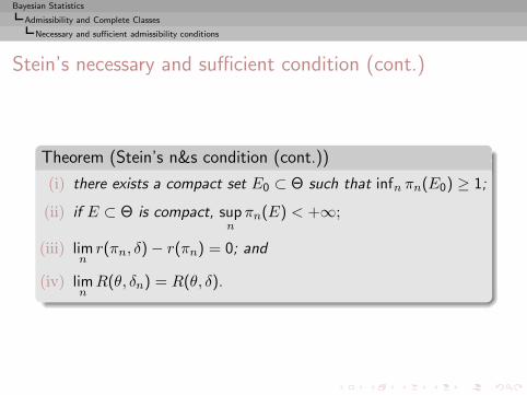
Bayesian Statistics
Admissibility and Complete Classes
Necessary and sufficient admissibility conditions
Stein’s necessary and sufficient condition (cont.)
Theorem (Stein’s n&s condition (cont.))
(i) there exists a compact set E0 ⊂ Θ such that infn πn(E0) ≥ 1;
(ii) if E ⊂ Θ is compact, supnπn(E) < +∞;
(iii) limnr(πn, δ) − r(πn) = 0; and
(iv) limnR(θ, δn) = R(θ, δ).
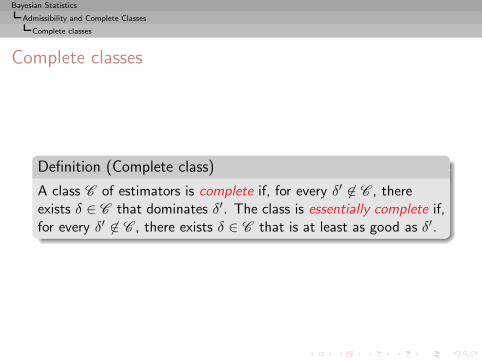
Bayesian Statistics
Admissibility and Complete Classes
Complete classes
Complete classes
Definition (Complete class)
A class C of estimators is complete if, for every δ′ 6∈ C , thereexists δ ∈ C that dominates δ′. The class is essentially complete if,for every δ′ 6∈ C , there exists δ ∈ C that is at least as good as δ′.
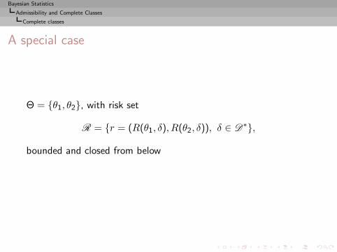
Bayesian Statistics
Admissibility and Complete Classes
Complete classes
A special case
Θ = {θ1, θ2}, with risk set
R = {r = (R(θ1, δ), R(θ2, δ)), δ ∈ D∗},
bounded and closed from below
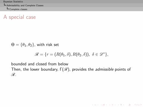
Bayesian Statistics
Admissibility and Complete Classes
Complete classes
A special case
Θ = {θ1, θ2}, with risk set
R = {r = (R(θ1, δ), R(θ2, δ)), δ ∈ D∗},
bounded and closed from belowThen, the lower boundary, Γ(R), provides the admissible points ofR.
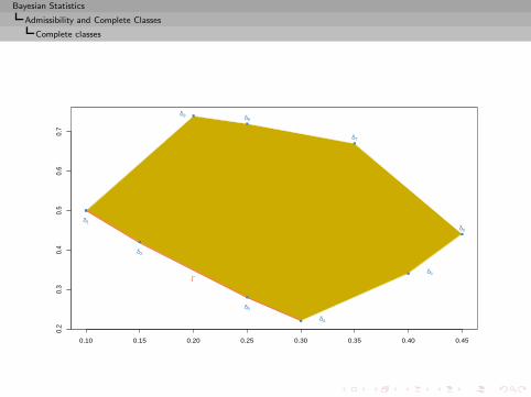
Bayesian Statistics
Admissibility and Complete Classes
Complete classes
0.10 0.15 0.20 0.25 0.30 0.35 0.40 0.45
0.2
0.3
0.4
0.5
0.6
0.7
δ1
δ2
δ3
δ4
δ5
δ6
δ7
δ8δ9
Γ
Bayesian Statistics
Admissibility and Complete Classes
Complete classes
A special case (cont.)
Reason
For every r ∈ Γ(R), there exists a tangent line to R going throughr, with positive slope and equation
p1r1 + p2r2 = k
Bayesian Statistics
Admissibility and Complete Classes
Complete classes
A special case (cont.)
Reason
For every r ∈ Γ(R), there exists a tangent line to R going throughr, with positive slope and equation
p1r1 + p2r2 = k
Therefore r is a Bayes estimator for π(θi) = pi (i = 1, 2)
Bayesian Statistics
Admissibility and Complete Classes
Complete classes
Wald’s theorems
Theorem
If Θ is finite and if R is bounded and closed from below, then theset of Bayes estimators constitutes a complete class
Bayesian Statistics
Admissibility and Complete Classes
Complete classes
Wald’s theorems
Theorem
If Θ is finite and if R is bounded and closed from below, then theset of Bayes estimators constitutes a complete class
Theorem
If Θ is compact and the risk set R is convex, if all estimators havea continuous risk function, the Bayes estimators constitute acomplete class.

Bayesian Statistics
Admissibility and Complete Classes
Complete classes
Extensions
If Θ not compact, in many cases, complete classes are made ofgeneralised Bayes estimators
Bayesian Statistics
Admissibility and Complete Classes
Complete classes
Extensions
If Θ not compact, in many cases, complete classes are made ofgeneralised Bayes estimators
Example
When estimating the natural parameter θ of an exponential family
x ∼ f(x|θ) = eθ·x−ψ(θ)h(x), x, θ ∈ Rk,
under quadratic loss, every admissible estimator is a generalisedBayes estimator.
Bayesian Statistics
Hierarchical and Empirical Bayes Extensions, and the Stein Effect
Hierarchical and Empirical Bayes Extensions
Introduction
Decision-Theoretic Foundations of Statistical Inference
From Prior Information to Prior Distributions
Bayesian Point Estimation
Bayesian Calculations
Tests and model choice
Admissibility and Complete Classes

Bayesian Statistics
Hierarchical and Empirical Bayes Extensions, and the Stein Effect
The Bayesian analysis is sufficiently reductive to produce effectivedecisions, but this efficiency can also be misused.

Bayesian Statistics
Hierarchical and Empirical Bayes Extensions, and the Stein Effect
The Bayesian analysis is sufficiently reductive to produce effectivedecisions, but this efficiency can also be misused.The prior information is rarely rich enough to define a priordistribution exactly.
Bayesian Statistics
Hierarchical and Empirical Bayes Extensions, and the Stein Effect
The Bayesian analysis is sufficiently reductive to produce effectivedecisions, but this efficiency can also be misused.The prior information is rarely rich enough to define a priordistribution exactly.
Uncertainty must be included within the Bayesian model:
◮ Further prior modelling
◮ Upper and lower probabilities [Dempster-Shafer]
◮ Imprecise probabilities [Walley]
Bayesian Statistics
Hierarchical and Empirical Bayes Extensions, and the Stein Effect
Hierarchical Bayes analysis
Hierarchical Bayes analysis
Decomposition of the prior distribution into several conditionallevels of distributions
Bayesian Statistics
Hierarchical and Empirical Bayes Extensions, and the Stein Effect
Hierarchical Bayes analysis
Hierarchical Bayes analysis
Decomposition of the prior distribution into several conditionallevels of distributions
Often two levels: the first-level distribution is generally a conjugateprior, with parameters distributed from the second-level distribution
Real life motivations (multiple experiments, meta-analysis, ...)
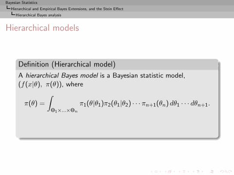
Bayesian Statistics
Hierarchical and Empirical Bayes Extensions, and the Stein Effect
Hierarchical Bayes analysis
Hierarchical models
Definition (Hierarchical model)
A hierarchical Bayes model is a Bayesian statistic model,(f(x|θ), π(θ)), where
π(θ) =
∫
Θ1×...×Θn
π1(θ|θ1)π2(θ1|θ2) · · · πn+1(θn) dθ1 · · · dθn+1.
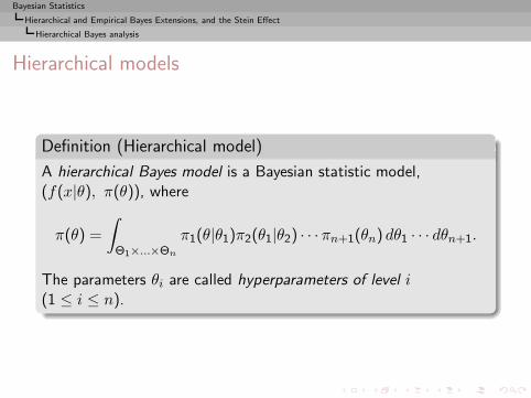
The parameters θi are called hyperparameters of level i(1 ≤ i ≤ n).
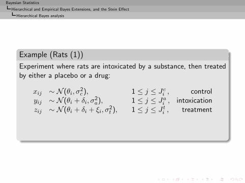
Bayesian Statistics
Hierarchical and Empirical Bayes Extensions, and the Stein Effect
Hierarchical Bayes analysis
Example (Rats (1))
Experiment where rats are intoxicated by a substance, then treatedby either a placebo or a drug:
xij ∼ N (θi, σ2c ), 1 ≤ j ≤ Jci , control
yij ∼ N (θi + δi, σ2a), 1 ≤ j ≤ Jai , intoxication
zij ∼ N (θi + δi + ξi, σ2t ), 1 ≤ j ≤ J ti , treatment
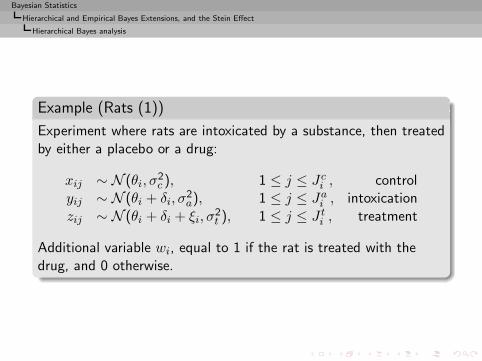
Additional variable wi, equal to 1 if the rat is treated with thedrug, and 0 otherwise.
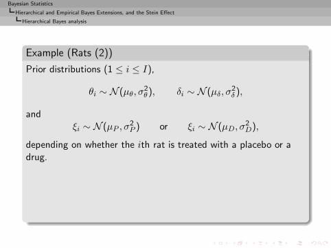
Bayesian Statistics
Hierarchical and Empirical Bayes Extensions, and the Stein Effect
Hierarchical Bayes analysis
Example (Rats (2))
Prior distributions (1 ≤ i ≤ I),
θi ∼ N (µθ, σ2θ), δi ∼ N (µδ, σ
2δ ),
andξi ∼ N (µP , σ
2P ) or ξi ∼ N (µD, σ
2D),
depending on whether the ith rat is treated with a placebo or adrug.
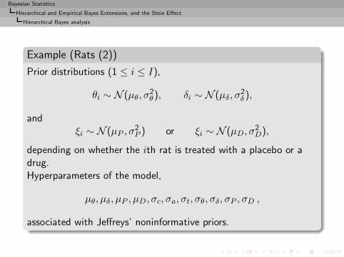
Bayesian Statistics
Hierarchical and Empirical Bayes Extensions, and the Stein Effect
Hierarchical Bayes analysis
Example (Rats (2))
Prior distributions (1 ≤ i ≤ I),
θi ∼ N (µθ, σ2θ), δi ∼ N (µδ, σ
2δ ),
andξi ∼ N (µP , σ
2P ) or ξi ∼ N (µD, σ
2D),
depending on whether the ith rat is treated with a placebo or adrug.Hyperparameters of the model,
µθ, µδ, µP , µD, σc, σa, σt, σθ, σδ, σP , σD ,
associated with Jeffreys’ noninformative priors.

Bayesian Statistics
Hierarchical and Empirical Bayes Extensions, and the Stein Effect
Hierarchical Bayes analysis
Justifications
1. Objective reasons based on prior information
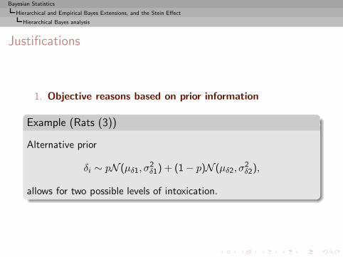
Bayesian Statistics
Hierarchical and Empirical Bayes Extensions, and the Stein Effect
Hierarchical Bayes analysis
Justifications
1. Objective reasons based on prior information
Example (Rats (3))
Alternative prior
δi ∼ pN (µδ1, σ2δ1) + (1 − p)N (µδ2, σ
2δ2),
allows for two possible levels of intoxication.
Bayesian Statistics
Hierarchical and Empirical Bayes Extensions, and the Stein Effect
Hierarchical Bayes analysis
2. Separation of structural information from subjectiveinformation
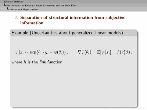
Bayesian Statistics
Hierarchical and Empirical Bayes Extensions, and the Stein Effect
Hierarchical Bayes analysis
2. Separation of structural information from subjectiveinformation
Example (Uncertainties about generalized linear models)
yi|xi ∼ exp{θi · yi − ψ(θi)} , ∇ψ(θi) = E[yi|xi] = h(xtiβ) ,
where h is the link function
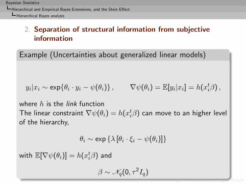
Bayesian Statistics
Hierarchical and Empirical Bayes Extensions, and the Stein Effect
Hierarchical Bayes analysis
2. Separation of structural information from subjectiveinformation
Example (Uncertainties about generalized linear models)
yi|xi ∼ exp{θi · yi − ψ(θi)} , ∇ψ(θi) = E[yi|xi] = h(xtiβ) ,
where h is the link functionThe linear constraint ∇ψ(θi) = h(xtiβ) can move to an higher levelof the hierarchy,
θi ∼ exp {λ [θi · ξi − ψ(θi)]}
with E[∇ψ(θi)] = h(xtiβ) and
β ∼ Nq(0, τ2Iq)

Bayesian Statistics
Hierarchical and Empirical Bayes Extensions, and the Stein Effect
Hierarchical Bayes analysis
3. In noninformative settings, compromise between theJeffreys noninformative distributions, and the conjugatedistributions.
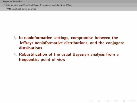
Bayesian Statistics
Hierarchical and Empirical Bayes Extensions, and the Stein Effect
Hierarchical Bayes analysis
3. In noninformative settings, compromise between theJeffreys noninformative distributions, and the conjugatedistributions.
4. Robustification of the usual Bayesian analysis from afrequentist point of view
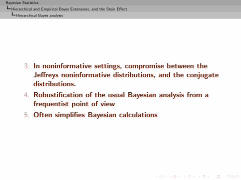
5. Often simplifies Bayesian calculations
Bayesian Statistics
Hierarchical and Empirical Bayes Extensions, and the Stein Effect
Hierarchical Bayes analysis
Conditional decompositions
Easy decomposition of the posterior distribution
Bayesian Statistics
Hierarchical and Empirical Bayes Extensions, and the Stein Effect
Hierarchical Bayes analysis
Conditional decompositions
Easy decomposition of the posterior distributionFor instance, if
θ|θ1 ∼ π1(θ|θ1), θ1 ∼ π2(θ1),
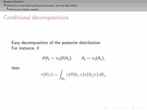
Bayesian Statistics
Hierarchical and Empirical Bayes Extensions, and the Stein Effect
Hierarchical Bayes analysis
Conditional decompositions
Easy decomposition of the posterior distributionFor instance, if
θ|θ1 ∼ π1(θ|θ1), θ1 ∼ π2(θ1),
then
π(θ|x) =
∫
Θ1
π(θ|θ1, x)π(θ1|x) dθ1,
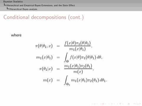
Bayesian Statistics
Hierarchical and Empirical Bayes Extensions, and the Stein Effect
Hierarchical Bayes analysis
Conditional decompositions (cont.)
where
π(θ|θ1, x) =f(x|θ)π1(θ|θ1)m1(x|θ1)
,
m1(x|θ1) =
∫
Θf(x|θ)π1(θ|θ1) dθ,
π(θ1|x) =m1(x|θ1)π2(θ1)
m(x),
m(x) =
∫
Θ1
m1(x|θ1)π2(θ1) dθ1.
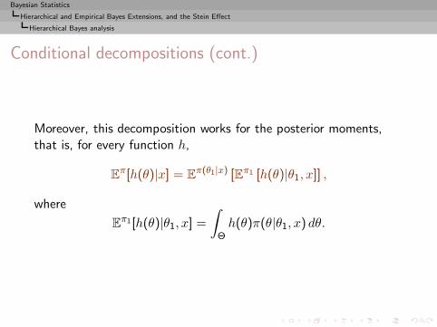
Bayesian Statistics
Hierarchical and Empirical Bayes Extensions, and the Stein Effect
Hierarchical Bayes analysis
Conditional decompositions (cont.)
Moreover, this decomposition works for the posterior moments,that is, for every function h,
Eπ[h(θ)|x] = E
π(θ1|x) [Eπ1 [h(θ)|θ1, x]] ,
where
Eπ1[h(θ)|θ1, x] =
∫
Θh(θ)π(θ|θ1, x) dθ.
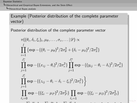
Bayesian Statistics
Hierarchical and Empirical Bayes Extensions, and the Stein Effect
Hierarchical Bayes analysis
Example (Posterior distribution of the complete parametervector)
Posterior distribution of the complete parameter vector
π((θi, δi, ξi)i, µθ, . . . , σc, . . . |D) ∝I∏
i=1
{exp−{(θi − µθ)
2/2σ2θ + (δi − µδ)
2/2σ2δ}
Jci∏
j=1
exp−{(xij − θi)2/2σ2
c}Ja
i∏
j=1
exp−{(yij − θi − δi)2/2σ2
a}
Jti∏
j=1
exp−{(zij − θi − δi − ξi)2/2σ2
t }}
∏
ℓi=0
exp−{(ξi − µP )2/2σ2P }∏
ℓi=1
exp−{(ξi − µD)2/2σ2D}
−P
Jc−1 −P
Ja−1 −P
Jt−1 −I−1 −I −1 −I −1
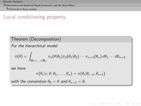
Bayesian Statistics
Hierarchical and Empirical Bayes Extensions, and the Stein Effect
Hierarchical Bayes analysis
Local conditioning property
Theorem (Decomposition)
For the hierarchical model
π(θ) =
∫
Θ1×...×Θn
π1(θ|θ1)π2(θ1|θ2) · · · πn+1(θn) dθ1 · · · dθn+1.
we haveπ(θi|x, θ, θ1, . . . , θn) = π(θi|θi−1, θi+1)
with the convention θ0 = θ and θn+1 = 0.
Bayesian Statistics
Hierarchical and Empirical Bayes Extensions, and the Stein Effect
Hierarchical Bayes analysis
Computational issues
Rarely an explicit derivation of the corresponding Bayes estimatorsNatural solution in hierarchical settings: use a simulation-basedapproach exploiting the hierarchical conditional structure
Example (Rats (4))
The full conditional distributions correspond to standarddistributions and Gibbs sampling applies.
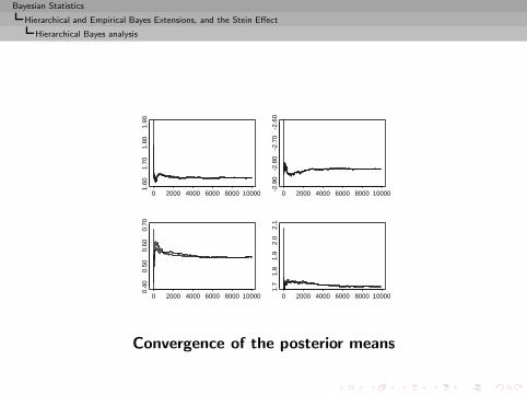
Bayesian Statistics
Hierarchical and Empirical Bayes Extensions, and the Stein Effect
Hierarchical Bayes analysis
0 2000 4000 6000 8000 10000
1.60
1.70
1.80
1.90
0 2000 4000 6000 8000 10000
-2.9
0-2
.80
-2.7
0-2
.60
0 2000 4000 6000 8000 10000
0.40
0.50
0.60
0.70
0 2000 4000 6000 8000 10000
1.7
1.8
1.9
2.0
2.1
Convergence of the posterior means
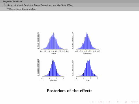
Bayesian Statistics
Hierarchical and Empirical Bayes Extensions, and the Stein Effect
Hierarchical Bayes analysis
1.0 1.2 1.4 1.6 1.8 2.0 2.2 2.4
020
4060
8010
0120
control
-4.0 -3.5 -3.0 -2.5 -2.0 -1.5
020
4060
8010
014
0
intoxication
-1 0 1 2
050
1001
5020
0250
300
placebo
0 1 2 3
050
1001
5020
0250
drug
Posteriors of the effects
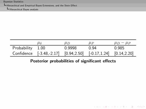
Bayesian Statistics
Hierarchical and Empirical Bayes Extensions, and the Stein Effect
Hierarchical Bayes analysis
µδ µD µP µD − µPProbability 1.00 0.9998 0.94 0.985Confidence [-3.48,-2.17] [0.94,2.50] [-0.17,1.24] [0.14,2.20]
Posterior probabilities of significant effects
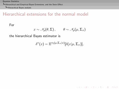
Bayesian Statistics
Hierarchical and Empirical Bayes Extensions, and the Stein Effect
Hierarchical Bayes analysis
Hierarchical extensions for the normal model
Forx ∼ Np(θ,Σ) , θ ∼ Np(µ,Σπ)
the hierarchical Bayes estimator is
δπ(x) = Eπ2(µ,Σπ|x)[δ(x|µ,Σπ)],
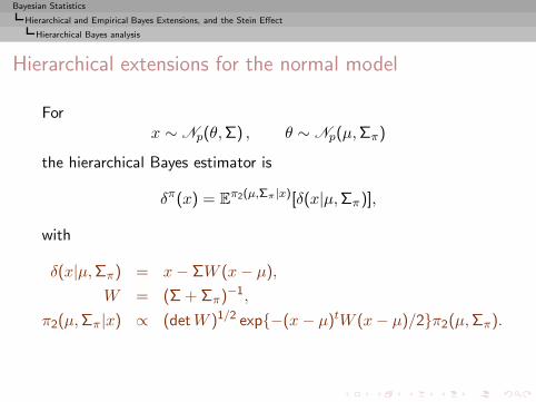
Bayesian Statistics
Hierarchical and Empirical Bayes Extensions, and the Stein Effect
Hierarchical Bayes analysis
Hierarchical extensions for the normal model
Forx ∼ Np(θ,Σ) , θ ∼ Np(µ,Σπ)
the hierarchical Bayes estimator is
δπ(x) = Eπ2(µ,Σπ|x)[δ(x|µ,Σπ)],
with
δ(x|µ,Σπ) = x− ΣW (x− µ),
W = (Σ + Σπ)−1,
π2(µ,Σπ|x) ∝ (detW )1/2 exp{−(x− µ)tW (x− µ)/2}π2(µ,Σπ).
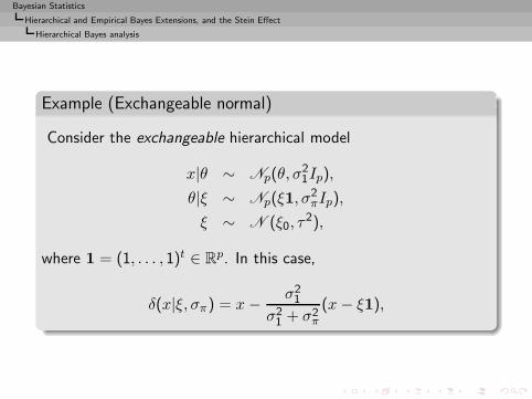
Bayesian Statistics
Hierarchical and Empirical Bayes Extensions, and the Stein Effect
Hierarchical Bayes analysis
Example (Exchangeable normal)
Consider the exchangeable hierarchical model
x|θ ∼ Np(θ, σ21Ip),
θ|ξ ∼ Np(ξ1, σ2πIp),
ξ ∼ N (ξ0, τ2),
where 1 = (1, . . . , 1)t ∈ Rp. In this case,
δ(x|ξ, σπ) = x− σ21
σ21 + σ2
π
(x− ξ1),
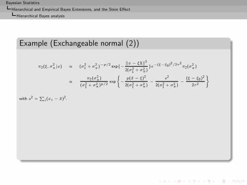
Bayesian Statistics
Hierarchical and Empirical Bayes Extensions, and the Stein Effect
Hierarchical Bayes analysis
Example (Exchangeable normal (2))
π2(ξ, σ2π|x) ∝ (σ
21 + σ
2π)
−p/2exp{−
‖x − ξ1‖2
2(σ21 + σ2
π)}e
−(ξ−ξ0)2/2τ2π2(σ
2π)
∝π2(σ2
π)
(σ21 + σ2
π)p/2exp
(
−p(x − ξ)2
2(σ21 + σ2
π)−
s2
2(σ21 + σ2
π)−
(ξ − ξ0)2
2τ2
)
with s2 =P
i(xi − x)2.
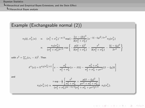
Bayesian Statistics
Hierarchical and Empirical Bayes Extensions, and the Stein Effect
Hierarchical Bayes analysis
Example (Exchangeable normal (2))
π2(ξ, σ2π|x) ∝ (σ
21 + σ
2π)
−p/2exp{−
‖x − ξ1‖2
2(σ21 + σ2
π)}e
−(ξ−ξ0)2/2τ2π2(σ
2π)
∝π2(σ2
π)
(σ21 + σ2
π)p/2exp
(
−p(x − ξ)2
2(σ21 + σ2
π)−
s2
2(σ21 + σ2
π)−
(ξ − ξ0)2
2τ2
)
with s2 =P
i(xi − x)2. Then
δπ
(x) = Eπ2(σ2
π|x)
"
x −σ2
1
σ21 + σ2
π
(x − x1) −σ2
1 + σ2π
σ21 + σ2
π + pτ2(x − ξ0)1
#
and
π2(σ2π|x) ∝
τ exp − 12
"
s2
σ21 + σ2
π
+p(x − ξ0)2
pτ2 + σ21 + σ2
π
#
(σ21 + σ2
π)(p−1)/2(σ21 + σ2
π + pτ2)1/2π2(σ
2π).
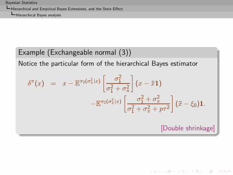
Bayesian Statistics
Hierarchical and Empirical Bayes Extensions, and the Stein Effect
Hierarchical Bayes analysis
Example (Exchangeable normal (3))
Notice the particular form of the hierarchical Bayes estimator
δπ(x) = x− Eπ2(σ
2π |x)
[σ2
1
σ21 + σ2
π
](x− x1)
−Eπ2(σ
2π |x)
[σ2
1 + σ2π
σ21 + σ2
π + pτ2
](x− ξ0)1.
[Double shrinkage]
Bayesian Statistics
Hierarchical and Empirical Bayes Extensions, and the Stein Effect
Hierarchical Bayes analysis
The Stein effect
If a minimax estimator is unique, it is admissible
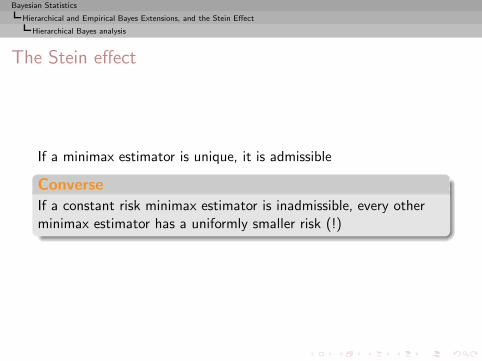
Bayesian Statistics
Hierarchical and Empirical Bayes Extensions, and the Stein Effect
Hierarchical Bayes analysis
The Stein effect
If a minimax estimator is unique, it is admissible
Converse
If a constant risk minimax estimator is inadmissible, every otherminimax estimator has a uniformly smaller risk (!)
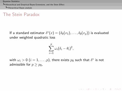
Bayesian Statistics
Hierarchical and Empirical Bayes Extensions, and the Stein Effect
Hierarchical Bayes analysis
The Stein Paradox
If a standard estimator δ∗(x) = (δ0(x1), . . . , δ0(xp)) is evaluatedunder weighted quadratic loss
p∑
i=1
ωi(δi − θi)2,
with ωi > 0 (i = 1, . . . , p), there exists p0 such that δ∗ is notadmissible for p ≥ p0,
Bayesian Statistics
Hierarchical and Empirical Bayes Extensions, and the Stein Effect
Hierarchical Bayes analysis
The Stein Paradox
If a standard estimator δ∗(x) = (δ0(x1), . . . , δ0(xp)) is evaluatedunder weighted quadratic loss
p∑
i=1
ωi(δi − θi)2,
with ωi > 0 (i = 1, . . . , p), there exists p0 such that δ∗ is notadmissible for p ≥ p0, although the components δ0(xi) areseparately admissible to estimate the θi’s.
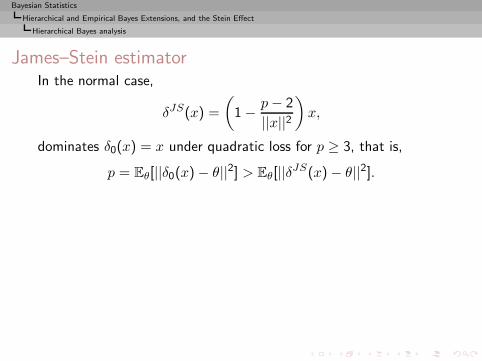
Bayesian Statistics
Hierarchical and Empirical Bayes Extensions, and the Stein Effect
Hierarchical Bayes analysis
James–Stein estimatorIn the normal case,
δJS(x) =
(1 − p− 2
||x||2)x,
dominates δ0(x) = x under quadratic loss for p ≥ 3, that is,
p = Eθ[||δ0(x) − θ||2] > Eθ[||δJS(x) − θ||2].
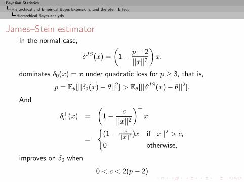
Bayesian Statistics
Hierarchical and Empirical Bayes Extensions, and the Stein Effect
Hierarchical Bayes analysis
James–Stein estimatorIn the normal case,
δJS(x) =
(1 − p− 2
||x||2)x,
dominates δ0(x) = x under quadratic loss for p ≥ 3, that is,
p = Eθ[||δ0(x) − θ||2] > Eθ[||δJS(x) − θ||2].And
δ+c (x) =
(1 − c
||x||2)+
x
=
{(1 − c
||x||2 )x if ||x||2 > c,
0 otherwise,
improves on δ0 when
0 < c < 2(p − 2)

Bayesian Statistics
Hierarchical and Empirical Bayes Extensions, and the Stein Effect
Hierarchical Bayes analysis
Universality
◮ Other distributions than the normal distribution
Bayesian Statistics
Hierarchical and Empirical Bayes Extensions, and the Stein Effect
Hierarchical Bayes analysis
Universality
◮ Other distributions than the normal distribution
◮ Other losses other than the quadratic loss
Bayesian Statistics
Hierarchical and Empirical Bayes Extensions, and the Stein Effect
Hierarchical Bayes analysis
Universality
◮ Other distributions than the normal distribution
◮ Other losses other than the quadratic loss
◮ Connections with admissibility
Bayesian Statistics
Hierarchical and Empirical Bayes Extensions, and the Stein Effect
Hierarchical Bayes analysis
Universality
◮ Other distributions than the normal distribution
◮ Other losses other than the quadratic loss
◮ Connections with admissibility
◮ George’s multiple shrinkage
Bayesian Statistics
Hierarchical and Empirical Bayes Extensions, and the Stein Effect
Hierarchical Bayes analysis
Universality
◮ Other distributions than the normal distribution
◮ Other losses other than the quadratic loss
◮ Connections with admissibility
◮ George’s multiple shrinkage
◮ Robustess against distribution
◮ Applies for confidence regions
◮ Applies for accuracy (or loss) estimation
◮ Cannot occur in finite parameter spaces
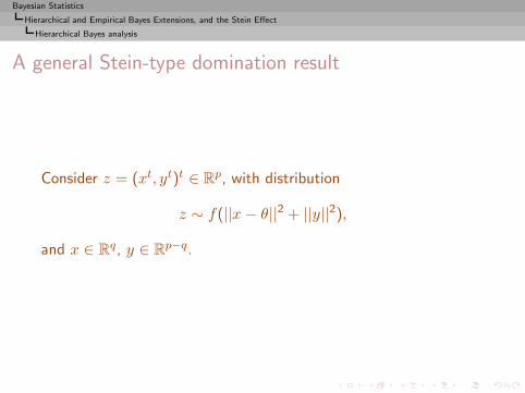
Bayesian Statistics
Hierarchical and Empirical Bayes Extensions, and the Stein Effect
Hierarchical Bayes analysis
A general Stein-type domination result
Consider z = (xt, yt)t ∈ Rp, with distribution
z ∼ f(||x− θ||2 + ||y||2),
and x ∈ Rq, y ∈ Rp−q.
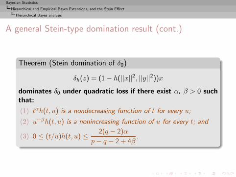
Bayesian Statistics
Hierarchical and Empirical Bayes Extensions, and the Stein Effect
Hierarchical Bayes analysis
A general Stein-type domination result (cont.)
Theorem (Stein domination of δ0)
δh(z) = (1 − h(||x||2, ||y||2))xdominates δ0 under quadratic loss if there exist α, β > 0 suchthat:
(1) tαh(t, u) is a nondecreasing function of t for every u;
(2) u−βh(t, u) is a nonincreasing function of u for every t; and
(3) 0 ≤ (t/u)h(t, u) ≤ 2(q − 2)α
p− q − 2 + 4β.
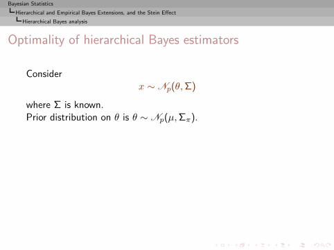
Bayesian Statistics
Hierarchical and Empirical Bayes Extensions, and the Stein Effect
Hierarchical Bayes analysis
Optimality of hierarchical Bayes estimators
Considerx ∼ Np(θ,Σ)
where Σ is known.Prior distribution on θ is θ ∼ Np(µ,Σπ).
Bayesian Statistics
Hierarchical and Empirical Bayes Extensions, and the Stein Effect
Hierarchical Bayes analysis
Optimality of hierarchical Bayes estimators
Considerx ∼ Np(θ,Σ)
where Σ is known.Prior distribution on θ is θ ∼ Np(µ,Σπ).The prior distribution π2 of the hyperparameters
(µ,Σπ)
is decomposed as
π2(µ,Σπ) = π12(Σπ|µ)π2
2(µ).
Bayesian Statistics
Hierarchical and Empirical Bayes Extensions, and the Stein Effect
Hierarchical Bayes analysis
Optimality of hierarchical Bayes estimators
In this case,
m(x) =
∫
Rp
m(x|µ)π22(µ) dµ,
with
m(x|µ) =
∫f(x|θ)π1(θ|µ,Σπ)π
12(Σπ|µ) dθ dΣπ.
Bayesian Statistics
Hierarchical and Empirical Bayes Extensions, and the Stein Effect
Hierarchical Bayes analysis
Optimality of hierarchical Bayes estimators
Moreover, the Bayes estimator
δπ(x) = x+ Σ∇ logm(x)
can be written
δπ(x) =
∫δ(x|µ)π2
2(µ|x) dµ,
with
δ(x|µ) = x+ Σ∇ logm(x|µ),
π22(µ|x) =
m(x|µ)π22(µ)
m(x).
Bayesian Statistics
Hierarchical and Empirical Bayes Extensions, and the Stein Effect
Hierarchical Bayes analysis
A sufficient condition
An estimator δ is minimax under the loss
LQ(θ, δ) = (θ − δ)tQ(θ − δ).
if it satisfies
R(θ, δ) = Eθ[LQ(θ, δ(x))] ≤ tr(ΣQ)
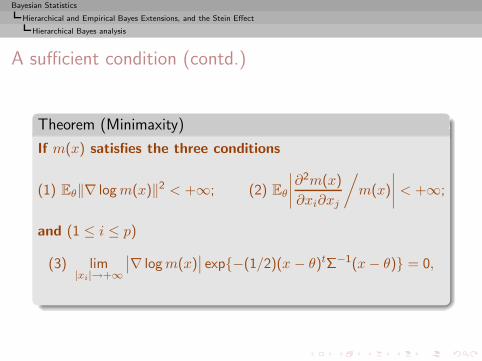
Bayesian Statistics
Hierarchical and Empirical Bayes Extensions, and the Stein Effect
Hierarchical Bayes analysis
A sufficient condition (contd.)
Theorem (Minimaxity)
If m(x) satisfies the three conditions
(1) Eθ‖∇ logm(x)‖2 < +∞; (2) Eθ
∣∣∣∣∂2m(x)
∂xi∂xj
/m(x)
∣∣∣∣ < +∞;
and (1 ≤ i ≤ p)
(3) lim|xi|→+∞
∣∣∇ logm(x)∣∣ exp{−(1/2)(x − θ)tΣ−1(x− θ)} = 0,
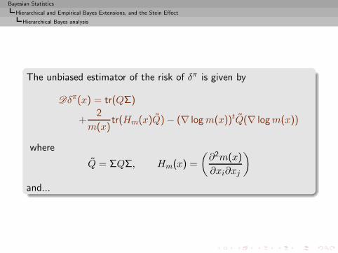
Bayesian Statistics
Hierarchical and Empirical Bayes Extensions, and the Stein Effect
Hierarchical Bayes analysis
The unbiased estimator of the risk of δπ is given by
Dδπ(x) = tr(QΣ)
+2
m(x)tr(Hm(x)Q) − (∇ logm(x))tQ(∇ logm(x))
where
Q = ΣQΣ, Hm(x) =
(∂2m(x)
∂xi∂xj
)
and...
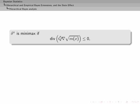
Bayesian Statistics
Hierarchical and Empirical Bayes Extensions, and the Stein Effect
Hierarchical Bayes analysis
δπ is minimax ifdiv(Q∇
√m(x)
)≤ 0,
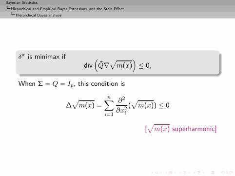
Bayesian Statistics
Hierarchical and Empirical Bayes Extensions, and the Stein Effect
Hierarchical Bayes analysis
δπ is minimax ifdiv(Q∇
√m(x)
)≤ 0,
When Σ = Q = Ip, this condition is
∆√m(x) =
n∑
i=1
∂2
∂x2i
(√m(x)) ≤ 0
[√m(x) superharmonic]
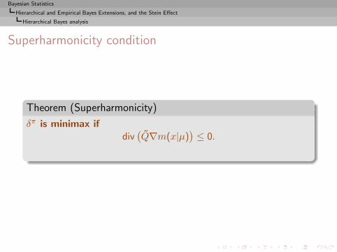
Bayesian Statistics
Hierarchical and Empirical Bayes Extensions, and the Stein Effect
Hierarchical Bayes analysis
Superharmonicity condition
Theorem (Superharmonicity)
δπ is minimax ifdiv(Q∇m(x|µ)
)≤ 0.
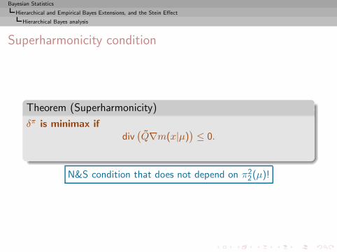
Bayesian Statistics
Hierarchical and Empirical Bayes Extensions, and the Stein Effect
Hierarchical Bayes analysis
Superharmonicity condition
Theorem (Superharmonicity)
δπ is minimax ifdiv(Q∇m(x|µ)
)≤ 0.
N&S condition that does not depend on π22(µ)!
Bayesian Statistics
Hierarchical and Empirical Bayes Extensions, and the Stein Effect
The empirical Bayes alternative
Empirical Bayes alternative
Strictly speaking, not a Bayesian method !
Bayesian Statistics
Hierarchical and Empirical Bayes Extensions, and the Stein Effect
The empirical Bayes alternative
Empirical Bayes alternative
Strictly speaking, not a Bayesian method !
(i) can be perceived as a dual method of the hierarchical Bayesanalysis;
(ii) asymptotically equivalent to the Bayesian approach;
(iii) usually classified as Bayesian by others; and
(iv) may be acceptable in problems for which a genuine Bayesmodeling is too complicated/costly.
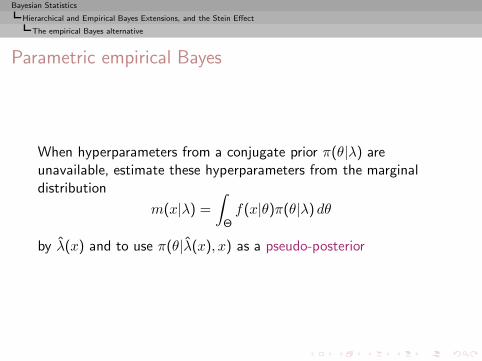
Bayesian Statistics
Hierarchical and Empirical Bayes Extensions, and the Stein Effect
The empirical Bayes alternative
Parametric empirical Bayes
When hyperparameters from a conjugate prior π(θ|λ) areunavailable, estimate these hyperparameters from the marginaldistribution
m(x|λ) =
∫
Θf(x|θ)π(θ|λ) dθ
by λ(x) and to use π(θ|λ(x), x) as a pseudo-posterior
Bayesian Statistics
Hierarchical and Empirical Bayes Extensions, and the Stein Effect
The empirical Bayes alternative
Fundamental ad-hocquery
Which estimate λ(x) for λ ?Moment method or maximum likelihood or Bayes or &tc...
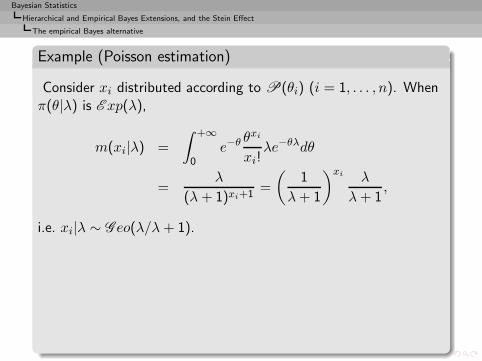
Bayesian Statistics
Hierarchical and Empirical Bayes Extensions, and the Stein Effect
The empirical Bayes alternative
Example (Poisson estimation)
Consider xi distributed according to P(θi) (i = 1, . . . , n). Whenπ(θ|λ) is E xp(λ),
m(xi|λ) =
∫ +∞
0e−θ
θxi
xi!λe−θλdθ
=λ
(λ+ 1)xi+1=
(1
λ+ 1
)xi λ
λ+ 1,
i.e. xi|λ ∼ G eo(λ/λ+ 1).
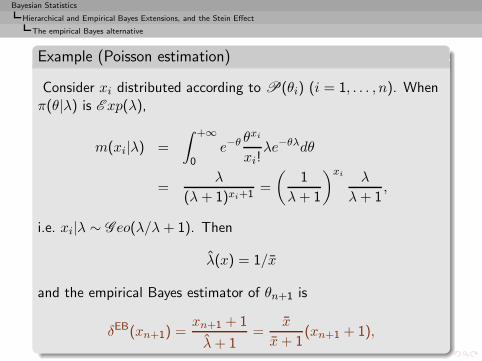
Bayesian Statistics
Hierarchical and Empirical Bayes Extensions, and the Stein Effect
The empirical Bayes alternative
Example (Poisson estimation)
Consider xi distributed according to P(θi) (i = 1, . . . , n). Whenπ(θ|λ) is E xp(λ),
m(xi|λ) =
∫ +∞
0e−θ
θxi
xi!λe−θλdθ
=λ
(λ+ 1)xi+1=
(1
λ+ 1
)xi λ
λ+ 1,
i.e. xi|λ ∼ G eo(λ/λ+ 1). Then
λ(x) = 1/x
and the empirical Bayes estimator of θn+1 is
δEB(xn+1) =xn+1 + 1
λ+ 1=
x
x+ 1(xn+1 + 1),
Bayesian Statistics
Hierarchical and Empirical Bayes Extensions, and the Stein Effect
The empirical Bayes alternative
Empirical Bayes justifications of the Stein effect
A way to unify the different occurrences of this paradox and showits Bayesian roots
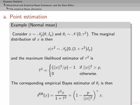
Bayesian Statistics
Hierarchical and Empirical Bayes Extensions, and the Stein Effect
The empirical Bayes alternative
a. Point estimation
Example (Normal mean)
Consider x ∼ Np(θ, Ip) and θi ∼ N (0, τ2). The marginaldistribution of x is then
x|τ2 ∼ Np(0, (1 + τ2)Ip)
and the maximum likelihood estimator of τ2 is
τ2 =
{(||x||2/p) − 1 if ||x||2 > p,
0 otherwise.
The corresponding empirical Bayes estimator of θi is then
δEB(x) =τ2x
1 + τ2=
(1 − p
||x||2)+
x.
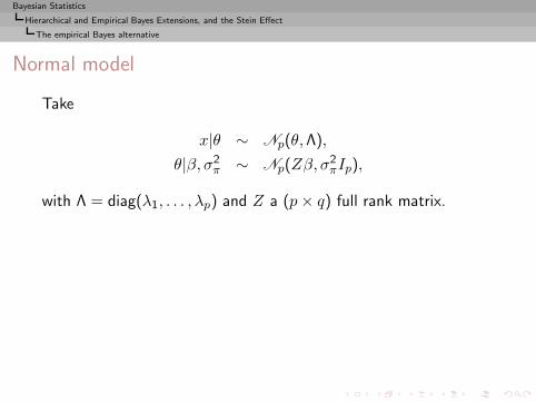
Bayesian Statistics
Hierarchical and Empirical Bayes Extensions, and the Stein Effect
The empirical Bayes alternative
Normal model
Take
x|θ ∼ Np(θ,Λ),
θ|β, σ2π ∼ Np(Zβ, σ
2πIp),
with Λ = diag(λ1, . . . , λp) and Z a (p× q) full rank matrix.
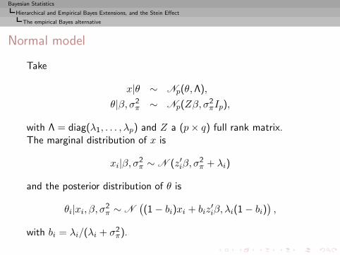
Bayesian Statistics
Hierarchical and Empirical Bayes Extensions, and the Stein Effect
The empirical Bayes alternative
Normal model
Take
x|θ ∼ Np(θ,Λ),
θ|β, σ2π ∼ Np(Zβ, σ
2πIp),
with Λ = diag(λ1, . . . , λp) and Z a (p× q) full rank matrix.The marginal distribution of x is
xi|β, σ2π ∼ N (z′iβ, σ
2π + λi)
and the posterior distribution of θ is
θi|xi, β, σ2π ∼ N
((1 − bi)xi + biz
′iβ, λi(1 − bi)
),
with bi = λi/(λi + σ2π).
Bayesian Statistics
Hierarchical and Empirical Bayes Extensions, and the Stein Effect
The empirical Bayes alternative
Normal model (cont.)
Ifλ1 = . . . = λn = σ2
the best equivariant estimators of β and b are given by
β = (ZtZ)−1Ztx and b =(p− q − 2)σ2
s2,
with s2 =∑p
i=1(xi − z′iβ)2.
Bayesian Statistics
Hierarchical and Empirical Bayes Extensions, and the Stein Effect
The empirical Bayes alternative
Normal model (cont.)
Ifλ1 = . . . = λn = σ2
the best equivariant estimators of β and b are given by
β = (ZtZ)−1Ztx and b =(p− q − 2)σ2
s2,
with s2 =∑p
i=1(xi − z′iβ)2.The corresponding empirical Bayes estimator of θ are
δEB(x) = Zβ +
(
1 − (p− q − 2)σ2
||x− Zβ||2
)
(x− Zβ),
which is of the form of the general Stein estimator
Bayesian Statistics
Hierarchical and Empirical Bayes Extensions, and the Stein Effect
The empirical Bayes alternative
Normal model (cont.)
When the means are assumed to be identical (exchangeability), thematrix Z reduces to the vector 1 and β ∈ R
Bayesian Statistics
Hierarchical and Empirical Bayes Extensions, and the Stein Effect
The empirical Bayes alternative
Normal model (cont.)
When the means are assumed to be identical (exchangeability), thematrix Z reduces to the vector 1 and β ∈ R
The empirical Bayes estimator is then
δEB(x) = x1 +
(1 − (p − 3)σ2
||x− x1||2)
(x− x1).
Bayesian Statistics
Hierarchical and Empirical Bayes Extensions, and the Stein Effect
The empirical Bayes alternative
b. Variance evaluation
Estimation of the hyperparameters β and σ2π considerably modifies
the behavior of the procedures.
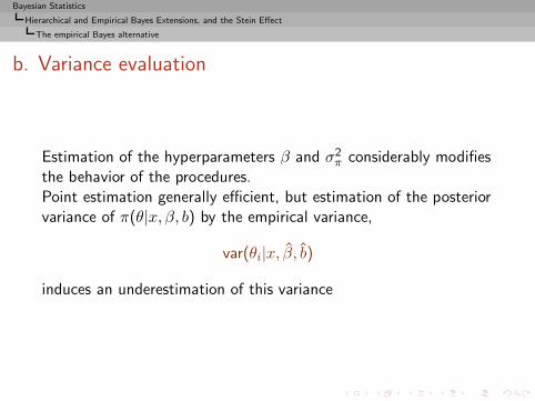
Bayesian Statistics
Hierarchical and Empirical Bayes Extensions, and the Stein Effect
The empirical Bayes alternative
b. Variance evaluation
Estimation of the hyperparameters β and σ2π considerably modifies
the behavior of the procedures.Point estimation generally efficient, but estimation of the posteriorvariance of π(θ|x, β, b) by the empirical variance,
var(θi|x, β, b)
induces an underestimation of this variance
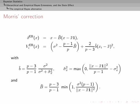
Bayesian Statistics
Hierarchical and Empirical Bayes Extensions, and the Stein Effect
The empirical Bayes alternative
Morris’ correction
δEB(x) = x− B(x− x1),
V EBi (x) =
(σ2 − p− 1
pB
)+
2
p− 3b(xi − x)2,
with
b =p− 3
p− 1
σ2
σ2 + σ2π
, σ2π = max
(0,
||x− x1||2p− 1
− σ2π
)
and
B =p− 3
p− 1min
(1,σ2(p− 1)
||x− x1||2).

Bayesian Statistics
A Defense of the Bayesian Choice
Unlimited range of applications
◮ artificial intelligence
◮ biostatistic
◮ econometrics
◮ epidemiology
◮ environmetrics
◮ finance

Bayesian Statistics
A Defense of the Bayesian Choice
◮ genomics
◮ geostatistics
◮ image processing and pattern recognition
◮ neural networks
◮ signal processing
◮ Bayesian networks
Bayesian Statistics
A Defense of the Bayesian Choice
rabicnameusec@enumi). Choosing a probabilistic representation
Bayesian Statistics appears as the calculus of uncertaintyReminder:A probabilistic model is nothing but an interpretation of agiven phenomenon
Bayesian Statistics
A Defense of the Bayesian Choice
rabicnameusec@enumi). Conditioning on the dataAt the basis of inference lies an inversion process betweencause and effect. Using a prior brings a necessary balancebetween observations and parameters and enable to operateconditional upon x
Bayesian Statistics
A Defense of the Bayesian Choice
rabicnameusec@enumi). Exhibiting the true likelihoodProvides a complete quantitative inference on the parametersand predictive that points out inadequacies of frequentiststatistics, while implementing the Likelihood Principle.

Bayesian Statistics
A Defense of the Bayesian Choice
rabicnameusec@enumi). Using priors as tools and summariesThe choice of a prior π does not require any kind ofbelief belief in this : rather consider it as a tool thatsummarizes the available prior and the uncertaintysurrounding this
Bayesian Statistics
A Defense of the Bayesian Choice
rabicnameusec@enumi). Accepting the subjective basis of knowledgeKnowledge is a critical confrontation between a prioris andexperiments. Ignoring these a prioris impoverishes analysis.

Bayesian Statistics
A Defense of the Bayesian Choice
We have, for one thing, to use a language andour language is entirely made of preconceived ideasand has to be so. However, these are unconsciouspreconceived ideas, which are a million times moredangerous than the other ones. Were we to assertthat if we are including other preconceived ideas,consciously stated, we would aggravate the evil! I donot believe so: I rather maintain that they wouldbalance one another.
Henri Poincare, 1902
Bayesian Statistics
A Defense of the Bayesian Choice
rabicnameusec@enumi). Choosing a coherent system of inferenceTo force inference into a decision-theoretic mold allows for aclarification of the way inferential tools should be evaluated,and therefore implies a conscious (although subjective) choiceof the retained optimality.Logical inference process Start with requested properties,i.e. loss function and prior , then derive the best solutionsatisfying these properties.
Bayesian Statistics
A Defense of the Bayesian Choice
rabicnameusec@enumi). Looking for optimal proceduresBayesian inference widely intersects with the three notions ofminimaxity, and equivariance. Looking for an optimal mostoften ends up finding a Bayes .Optimality is easier to attain through the Bayes “filter”
Bayesian Statistics
A Defense of the Bayesian Choice
rabicnameusec@enumi). Solving the actual problemFrequentist methods justified on a long-term basis, i.e., fromthe statistician viewpoint. From a decision-maker’s point ofview, only the problem at hand matters! That is, he/she callsfor an inference conditional on x.
Bayesian Statistics
A Defense of the Bayesian Choice
rabicnameusec@enumi). Providing a universal system of inferenceGiven the three factors
(X , f(x|θ), (Θ, π(θ)), (D ,L(θ, d)) ,
the Bayesian approach validates one and only one inferentialprocedure
Bayesian Statistics
A Defense of the Bayesian Choice
rabicnameusec@enumi). Computing procedures as a minimization problemBayesian procedures are easier to compute than procedures ofalternative theories, in the sense that there exists a universalmethodmethod!universal for the computation of BayesestimatorsIn practice, the effective calculation of the Bayes estimators isoften more delicate but this defect is of another magnitude.