Bayesian Structured Prediction using

Gaussian Processes

Sebastien Bratieres, Novi Quadrianto and Zoubin GhahramaniDepartment of Engineering, University of Cambridge, UK

Abstract

We introduce a conceptually novel structured prediction model, GP-struct, which is kernelized, non-parametric and Bayesian, by design. Wemotivate the model with respect to existing approaches, among others,conditional random fields (CRFs), maximum margin Markov networks(M3N), and structured support vector machines (SVMstruct), which em-body only a subset of its properties. We present an inference procedurebased on Markov Chain Monte Carlo. The framework can be instantiatedfor a wide range of structured objects such as linear chains, trees, grids,and other general graphs. As a proof of concept, the model is bench-marked on several natural language processing tasks and a video gesturesegmentation task involving a linear chain structure. We show predictionaccuracies for GPstruct which are comparable to or exceeding those ofCRFs and SVMstruct.

1 Introduction

Much interesting data does not reduce to points, scalars or single categories.Images, DNA sequences and text, for instance, are not just structured objectscomprising simpler indendent atoms (pixels, DNA bases and words). The in-terdependencies among the atoms are rich and define many of the attributesrelevant to practical use. Suppose that we want to label each pixel in an imageas to whether it belongs to background or foreground (image segmentation), orwe want to decide whether DNA bases are coding or not. The output interde-pendencies suggest that we will perform better in these tasks by considering thestructured nature of the output, rather than solving a collection of independentclassification problems.

Existing statistical machine learning models for structured prediction, suchas maximum margin Markov Network (M3N) [1], structured support vector ma-chines (SVMstruct) [2] and conditional random field (CRF) [3], have establishedthemselves as the state-of-the-art solutions for structured problems (cf. figure1 and table 1 for a schematic representation of model relationships).

In this paper, we focus our attention on CRF-like models due to their prob-abilistic nature, which allows us to incorporate prior knowledge in a seamless

1

arX

iv:1

307.

3846

v1 [

stat

.ML

] 1

5 Ju

l 201

3

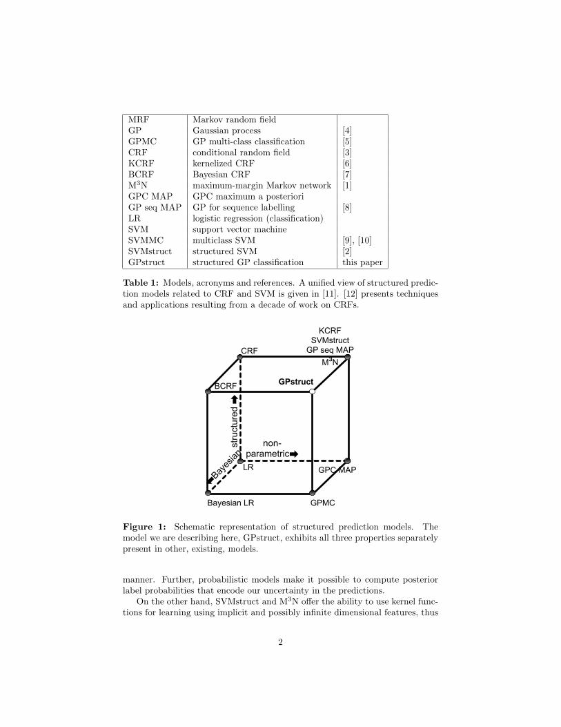
MRF Markov random fieldGP Gaussian process [4]GPMC GP multi-class classification [5]CRF conditional random field [3]KCRF kernelized CRF [6]BCRF Bayesian CRF [7]M3N maximum-margin Markov network [1]GPC MAP GPC maximum a posterioriGP seq MAP GP for sequence labelling [8]LR logistic regression (classification)SVM support vector machineSVMMC multiclass SVM [9], [10]SVMstruct structured SVM [2]GPstruct structured GP classification this paper

Table 1: Models, acronyms and references. A unified view of structured predic-tion models related to CRF and SVM is given in [11]. [12] presents techniquesand applications resulting from a decade of work on CRFs.

KCRFSVMstruct

GP seq MAPM³N

GPC MAP

GPMCBayesian LR

BCRF

LR

CRF

GPstruct

non-parametric�

�Bay

esian

stru

ctur

ed �

Figure 1: Schematic representation of structured prediction models. Themodel we are describing here, GPstruct, exhibits all three properties separatelypresent in other, existing, models.

manner. Further, probabilistic models make it possible to compute posteriorlabel probabilities that encode our uncertainty in the predictions.

On the other hand, SVMstruct and M3N offer the ability to use kernel func-tions for learning using implicit and possibly infinite dimensional features, thus

2

overcoming the drawbacks of finite dimensional parametric models such as theCRF. In addition, kernel combination allows the integration of multiple sourcesof information in a principled manner. These reasons motivate introducingMercer kernels in CRFs [6], an advantage that we wish to maintain.

From training and inference point of views, most CRF models estimate theirparameters point-wise using some form of optimisation. In contrast, [7] providea Bayesian treatment of the CRF which approximates the posterior distributionof the model parameters, in order to subsequently average over this distributionat prediction time. This method avoids important issues such as overfitting, orthe necessity of cross-validation for model selection.

Reflecting on this rich history of CRF models, we ask a very natural question:can we have a CRF model which is able to use implicit features spaces and atthe same time estimates a posterior distribution over model parameters? Themain drive for pursuing this direction is to combine the best of both worlds fromKernelized CRFs and Bayesian CRFs. To achieve this, we investigate the use ofGaussian processes (GP) [4] for modelling structured data where the structureis imposed by a Markov Random Field as in the CRF.

Our contributions are the following:

• a conceptually novel model which combines GPs and CRFs, and its co-herent and general formalisation;

• while the structure in the model is imposed by a Markov Random Field,which is very general, as a proof of concept we investigate a linear chaininstantiation;

• a Bayesian learning algorithm which is able to address model selectionwithout the need of cross-validation, a drawback of many popular struc-tured prediction models;

The present paper is structured as follows. Section 2 describes the modelitself, its parameterization and its application to sequential data, following upwith our proposed learning algorithm in section 3. In section 4, we situate ourmodel with respect to existing structured prediction models. An experimentalevaluation against other models suited to the same task is discussed in section5.

2 The model

The learning problem addressed in the present paper is structured prediction.Assume data consists of observation-label (or input-output) tuples, which wewill note D = {(x(1),y(1)), . . . , (x(N),y(N))}, where N is the size of the dataset,and (x(n),y(n)) ∈ X×Y is a data point. In the structured context, y is an objectsuch as a sequence, a grid, or a tree, which exhibits structure in the sense thatit consists of interdependent categorical atoms. Sometimes the output y isreferred to as the macro-label, while its constituents are termed micro-labels.The observation (input) x may have some structure of its own. Often, the

3

structure of y then reflects the structure of x, so that parts of the label mapto parts of the observation, but this is not required. The goal of the learningproblem is to predict labels for new observations.

The model we introduce here, which we call GPstruct, in analogy to thestructured support vector machine (SVMstruct) [2], can be succinctly describedas follows. Latent variables (LV) mediate the influence of the input on theoutput. The distribution of the output labels given the input and the LV isdefined per clique: in undirected graphical models, a clique is a set of nodessuch that every two nodes are connected. Let this distribution be:

p(y|x, f) =exp(

∑c f(c,xc,yc))∑

y′∈Y exp(∑c f(c,xc,y′c))

(1)

where yc and xc are tuples of nodes belonging to clique c, while f(c,xc,yc) isa LV associated with this particular clique and values for nodes xc and yc. Letf be the collection of all LV of the form f(c,xc,yc). We call the distribution(1) structured softmax, in analogy to the softmax (a.k.a. multinomial logistic)likelihood used in multinomial logistic regression. The conditional distributionin (1) is essentially a CRF over the input-output pairs, where the potentialfor each clique c is given by a Gibbs distribution, whose energy function isE(x,y) =

∑c−f(c,xc,yc).

In the CRF, potentials are log-linear in the parameters, with basis functionwTφc(xc,yc), where w is the weight parameter and φc a feature extractionfunction. Here instead, rather than choosing parametric clique potentials asin the CRF, the GPstruct model assumes that f(c,xc,yc) is a non-parametricfunction of its arguments, and gives this function a GP prior. Note that wesubstitute not only w, but the entire basis function by a LV. In particular,f(c,xc,yc) is drawn from a GP with covariance function (i.e. Mercer kernel)k((c,xc,yc), (c

′,xc′ ,yc′)), so that:

f ∼ GP(0, k(·, ·)) (2)

In summary, the GPstruct is a probabilistic model in which the likelihood isgiven by a structured softmax, with a Markov random field (MRF) modellingoutput interdependencies; the MRF’s LV, one per factor, are given a GP prior.This MRF could take on many shapes: linear for text, grid-shaped to labelpixels in computer vision tasks [13], or even, to take a less trivial example,hierarchical, in order to model probabilistic context-free grammars in a naturallanguage parsing task using CRFs [14].

2.1 Linear chain parameterization

While this model is very general, we will now instantiate it for the case of sequen-tial data, on which our experiments are based. Both the input and output con-sist of a linear chain of equal length T , and where the micro-labels all stem froma common set, i.e. Y = ×

t=1,...,TYt with ∀t,Yt = L (and the same for X and Xt).

4

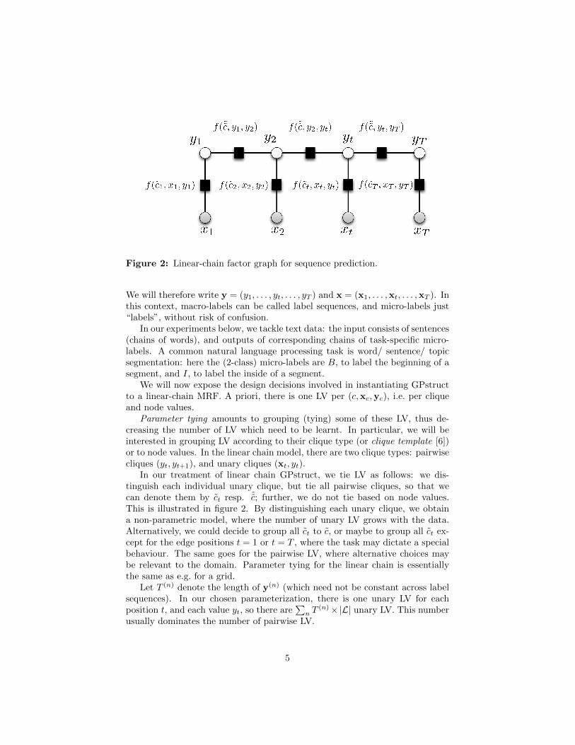
Figure 2: Linear-chain factor graph for sequence prediction.

We will therefore write y = (y1, . . . , yt, . . . , yT ) and x = (x1, . . . ,xt, . . . ,xT ). Inthis context, macro-labels can be called label sequences, and micro-labels just“labels”, without risk of confusion.

In our experiments below, we tackle text data: the input consists of sentences(chains of words), and outputs of corresponding chains of task-specific micro-labels. A common natural language processing task is word/ sentence/ topicsegmentation: here the (2-class) micro-labels are B, to label the beginning of asegment, and I, to label the inside of a segment.

We will now expose the design decisions involved in instantiating GPstructto a linear-chain MRF. A priori, there is one LV per (c,xc,yc), i.e. per cliqueand node values.

Parameter tying amounts to grouping (tying) some of these LV, thus de-creasing the number of LV which need to be learnt. In particular, we will beinterested in grouping LV according to their clique type (or clique template [6])or to node values. In the linear chain model, there are two clique types: pairwisecliques (yt, yt+1), and unary cliques (xt, yt).

In our treatment of linear chain GPstruct, we tie LV as follows: we dis-tinguish each individual unary clique, but tie all pairwise cliques, so that wecan denote them by ct resp. ˜c; further, we do not tie based on node values.This is illustrated in figure 2. By distinguishing each unary clique, we obtaina non-parametric model, where the number of unary LV grows with the data.Alternatively, we could decide to group all ct to c, or maybe to group all ct ex-cept for the edge positions t = 1 or t = T , where the task may dictate a specialbehaviour. The same goes for the pairwise LV, where alternative choices maybe relevant to the domain. Parameter tying for the linear chain is essentiallythe same as e.g. for a grid.

Let T (n) denote the length of y(n) (which need not be constant across labelsequences). In our chosen parameterization, there is one unary LV for eachposition t, and each value yt, so there are

∑n T

(n)×|L| unary LV. This numberusually dominates the number of pairwise LV.

5

Note that we had to define LV for all possible labels yt (more generally,∀y ∈ Y), not just the ones observed. This is because in (1), the normalisationruns over y′ ∈ Y, and also because we want to evaluate p(y|x, f) for any potentialy. By contrast, the input x and therefore xt is always assumed observed in oursupervised setting, and so we do not need to define LV for ranges of xt values.

Now turning to pairwise LV: there is one pairwise LV per (yt, yt+1) tuple;

and so there are |Yt| × |Yt+1| = |L|2 pairwise LV.

2.2 Kernel function specification

The Gaussian process prior defines a multivariate Gaussian density over anysubset of the LV, with usually zero mean and a covariance function given by thepositive definite kernel (Mercer kernel) k [15]. Our choice of kernel decomposesinto a unary and pairwise kernel function:

k((c,xc,yc), (c′,xc′ ,yc′)) =

I[c, c′ ∈ {ct|t}] ku((t,xt, yt), (t′,xt′ , yt′))

+ I[c = c′ = ˜c] kp((ys, ys+1), (ys′ , ys′+1)) (3)

In the above, we make use of Iverson’s bracket notation: I[P ] = 1 when conditionP is true and 0 otherwise. The positions of c, c′ are noted t, t′, and xt,xt′ , yt, yt′

are the corresponding input resp. output node values.We give the unary kernel the form

ku((t,xt, yt), (t′,xt′ , yt′)) = I[yt = yt′ ]kx(xt,xt′). (4)

kx is an “input-only” kernel, for instance the linear kernel 〈xt,xt′〉, or thesquared exponential kernel, defined as the inverse of the exponentiated Eu-clidean distance: exp(− 1

γ ||xt − xt′ ||2), where γ is a kernel hyperparameter.Further, our pairwise kernel takes on the form

kp((yt, yt+1), (yt′ , yt′+1)) = I[yt = yt′ ∧ yt+1 = yt′+1] (5)

With the proper ordering of LV, the Gram matrix has a block-diagonalstructure:

K = cov[f ] =

(Kunary 0

0 Kpairwise

)(6)

It is a square matrix, of length equal to the total number of LV∑n T

(n)×|L|+|L|2. Kunary is block diagonal, with |L| equal square blocks, each the Gram

matrix of kx of size∑n T

(n), and Kpairwise = I|L|2 .

Summing up sections 2 to 2.2, designing an instance of a GPstruct modelrequires three types of decisions: the choice of the MRF, mainly dictated by thetask and the output data structure; parameter tying; kernel design. The nextsection now details attractive properties of this model.

6

2.3 Model properties

The GPstruct model has the following appealing statistical properties:Structured: the output structure is controlled by the design of the MRF,

which is very general. The only practical limitation is the availability of efficientinference procedures on the MRF.

Non-parametric: the number of LV grows with the size of the data. Inthe linear chain case, it is the number of unary LV which grows with the totallength of input sequences.

Bayesian: this is a probabilistic model that supports Bayesian inference,with the usual benefits of Bayesian learning. At prediction time: error bars andreject options. At learning time: model selection and hyperparameter learningwith inbuilt Occam’s razor effect, without the need for cross-validation.

Kernelized: a joint (input-output) kernel is defined over the LV. Kernelspotentially introduce several hyperparameters, making grid search for cross-validation intractable. Kernelized Bayesian models like GPstruct do not sufferfrom this, as they define a posterior over the hyperparameters.

3 Learning

Our learning algorithms are Markov chain Monte Carlo procedures, and as suchare “any-time”, in that they have no predefined stopping criterion.

3.1 Prediction

Given an unseen test point x∗, and assuming the LV f∗ corresponding to x∗ tobe accessible, we wish to predict label y∗ with lowest loss. Now, given f∗, theunderlying MRF is fully specified. In tree-shaped structures, belief propagationgives an exact answer in linear time O(T ); in the linear chain case, under 0/1loss `(y, y) = δ(y = y), we predict the jointly most probable output sequenceobtained from the Viterbi procedure, and under Hamming (micro-label-wise)error `(y, y) =

∑t δ(yt = yt), we predict the micro-label-wise most probable

output sequence. For other cases than trees, where exact inference is impos-sible, approximate inference methods such as loopy belief propagation [16] areavailable.

Given f , due to the GP marginalisation property, the test point LV f∗ aredistributed according to a multivariate Gaussian distribution (cf. e.g. [17, section2] for a derivation): f∗|f ∼ N(KT

∗ K−1f ,K∗∗ − KT

∗ K−1K∗), where matrices

K,K∗,K∗∗ have their element (i, j) equal to k(f i, f (j)) resp. k(f i, f(j)∗ ) resp.

k(f(i)∗ , f

(j)∗ ), with k the kernel described section 2.2.

Uncertainty over f∗|f is accounted for correctly by Bayesian model averaging :y∗ = arg maxy∗∈Y∗ p(y∗|f), with

p(y∗|f) =1

Nf∗|f

∑f∗|f

p(y∗|f∗) (7)

7

where Nf∗|f is the number of samples from f∗|f .

3.2 Sampling from the posterior

We wish to represent the posterior distribution f |D (as opposed to performinga MAP approximation of the posterior to a single value fMAP ). The trainingdata likelihood is p(D|f) =

∏n p(y

(n)|f ,x(n)), with the single point likelihoodgiven by (1). Training aims at maximizing the likelihood, for which we proposeto use elliptical slice sampling (ESS) [18], an efficient MCMC procedure for MLtraining of tightly coupled LV with a Gaussian prior. In all our experimentsbelow, we discard the first third of the samples before carrying out prediction,to allow for burn-in of the MCMC chain.

The computation of the likelihood itself is a non-trivial problem due to thepresence of the normalising constant, which ranges over y′ ∈ Y, of size expo-nential in the number of micro-labels |L|. In the case of tree-shaped MRFs,however, belief propagation yields an exact and usually efficient procedure; inthe linear case, it is referred to as forwards-backwards procedure, and runs inO(T |L|2).

ESS requires computing the full kernel matrix, of size O(N2LV ), where NLV

is the total number of LV, and its Cholesky, obtained in O(N2LV ) time steps.

The large size of the matrices is a limiting factor to our implementation.ESS yields samples of the posterior. To perform prediction, it is necessary

to introduce one more level of Bayesian model averaging: continuing from (7),p(y∗|D) = 1

Nf

∑f p(y∗|f) where Nf is the number of samples of f |D available.

4 Relation to other models

Our proposed method builds upon a large body of existing models, none ofwhich, however, exhibit all properties mentioned in section 2.3.

4.1 GP classification

Gaussian process models (or any regression models such as a linear regression)can be applied to classification problems. In a probabilistic approach to clas-sification, the goal is to model posterior probabilities of an input point x be-longing to one of |L| classes, y ∈ {1, . . . , |L|}. For binary classification (thatis |L| = 2), we can turn the output of a Gaussian process (in R) into a classprobability (in the interval [0, 1]) by using an appropriate non-linear activa-tion function. The most commonly used such function is the logistic function

p(y = 1|f,x) = exp(f(x))exp(f(x))+exp(−f(x)) . The resulting classification model is called

GP binary classification [5]. Let us now move from binary classification tomulti-class classification. This is achieved by maintaining K regression models,each model being indexed by a latent function fk. We use the vector notationf = (f1 . . . fK) to index the collection of latent functions. The desired multi-classmodel is obtained by using a generalisation of the logistic to multiple variables,

8

the softmax function: p(y = k|f ,x) = exp(fk(x))∑Kk=1 exp(fk(x))

. The corresponding model

is called Gaussian process multi-class classification (GPMC) [5]. Note that theabove multiclass distribution is normalised over the set of possible output labelsL (here |Y| = K). Simply extending the multi-class model for a structured pre-diction case is computationally infeasible due to the sheer size of the label setL. We provide a novel extension of Gaussian process for structured problems.Structured prediction itself has a long history of successful methods, which wediscuss in subsequent sections.

4.2 From logistic to structured logistic

A natural way to cater for interdependencies between micro-labels at predic-tion time, is to define an MRF over y, and to condition the resulting dis-tribution on the input x (i.e. in a graphical model representation, insert-ing directed edges from input to output): we thus obtain a mixed graphi-cal model, the conditional random field (CRF) [3], a very popular and suc-cessful model for structured prediction. The CRF defines a log-linear modelfor p(y|x): p(y|x,w) = 1

Z(x,w) exp (∑c 〈wc, φ(xc,yc)〉) , for a weight vector

w, and a joint input-output feature representation φ(x,y). In the above,Z(x,w) =

∑y′∈L

∏c exp(〈wc, φ(xc,yc)〉) is the normalising constant. As be-

fore, we use c to denote a clique. Instead of parameterizing the energy function,E(x,y) := −〈wc, φ(xc,yc)〉, by means of a weight vector, GPstruct place aGaussian process prior over energy functions, effectively side-stepping param-eterization. Recent advances in CRF modelling by [19] also side-step linearparameterization of the energy function. Instead, a random forest is used tomodel the energy function, allowing higher order interactions.

4.3 Kernelizing structured logistic

[6] presents a kernelized variant of the CRF, the kernel conditional random field(KCRF), where a kernel is defined over clique templates. The kernelized ver-sion of the CRF is generally difficult to construct, to train, and have severalhyperparameters that need to be set via cross-validation, therefore, have notbeen adopted as enthusiastically as regular CRF. Structured support vector ma-chines [2], SVMstruct, and maximum margin Markov networks [1], M3N alsomodel p(y|x) as a log-linear function. However, to learn w, while traditionalCRF learning maximizes the conditional log likelihood of the training data,both SVMstruct and M3N perform maximum margin training: learn w whichpredicts the correct outputs with a large margin compared to incorrect outputs(all other outputs except the correct ones). SVMstruct can be easily kernelizedby means of the representer theorem. Our proposed GPstruct is also kernelized,with a practical advantage that kernel hyperparameters can be inferred fromthe data instead of requiring a cross-validation procedure.

9

4.4 Bayesian versus MAP inference

By Bayesian inference (as opposed to maximum likelihood ML or maximum aposteriori MAP inference), we mean the preservation of the uncertainty overLV, that is their representation, not as point-wise estimates, but as randomvariables and their probability distribution.

CRF parameters are usually estimated point-wise, e.g. often with an MLor MAP objective using gradient ascent or approximate likelihood techniques,cf. [12] for a review. An exception to this is Bayesian conditional random field(BCRF) proposed by [7]. Instead of point-wise parameter estimation, the BCRFapproximates the posterior distribution of the CRF parameters as Gaussiandistributions and learns them using expectation propagation [20]. GPstructalso follows a Bayesian inference procedure, and combines it with kernelization.

Despite the similarity in name, the model in [8] is more similar to the KCRFthan to GPstruct. Like KCRF, this work tackles sequence labelling, while wepurposefully formulate GPstruct to apply to any underlying MRF, even thoughwe demonstrate its instantiation in sequences. More importantly, [8] take aMAP estimation of the LV, making the model, among others, unable to inferassociated hyperparameters directly from the data. However, the point-wiseMAP estimate comes with a benefit: sparsification, due to the applicability ofthe representer theorem. The LV appear as a weighted sum of kernel evaluationsover the data. Two methods are applicable from here. The first, applied in[8, 4.2] and [6, 3], consists in greedily selecting the LV/ clique associated tothe direction of steepest gradient, during the optimisation phase. The secondmethod consists of applying the “Taskar trick” [1], and is concerned with the factthat in the LV expression obtained from the representer theorem, the sum runsover Y, i.e. all possible macro-labels, which is exponentially large in |L|. Thistrick consists in a rearrangement of terms inside the objective functions whichallows a lower-dimensional reparameterization. These sparsification techniquesare not accessible to us due to the use of a Bayesian representation; howeveralternative techniques may come from the GP sparsification literature.

4.5 Structured prediction via output kernels

All previously mentioned structured prediction methods explicitly model theoutput interdependency via MRF. A different strand of work aims at buildingan implicit model of output correlations via a kernel similarity measure [21, 22].The twin Gaussian processes of [22] address structured continuous-output prob-lems by forcing input kernels to be similar to output kernels. This objectivereflects the assumption that similar inputs should produce similar outputs. Theinput and output are separately modelled by GPs with different kernels. Learn-ing consists of minimising KL divergence.

10

5 Applications

In order to appreciate how the proposed model and learning scheme compareto existing techniques, we conducted benchmark experiments on a range of lan-guage processing tasks: segmentation, chunking, and named entity recognition,as well as on a video processing task, gesture segmentation, all involving a linearchain structure.

5.1 Text Processing Task

Our data and tasks comes from the CRF++ toolbox1. Four standard naturallanguage processing tasks are available, cf. table 2. Noun phrase identification(Base NP) tags words occurring in noun phrases with B for beginning, I for aword inside a noun phrase, and O for other words. Chunking (i.e. shallow pars-ing) labels sentence constituents. The Segmentation task identifies words (thesegments) in sequences of Chinese ideograms. Japanese named entity recogni-tion (Japanese NE) labels several types of named entities (organisation, person,etc.) occurring in text.

The data was used in pre-processed form, with sparse binary features ex-tracted for each word position in each sentence. Results were averaged over fiveexperiments per task. Each experiment’s training and test data was extractedfrom the full data set (sizes given in table 2) so that the training sets were alwaysdisjoint – except in the case of segmentation, a small-data set of 36 sentencesoverall, which was subjected to five random splits.

Baselines We compared GPstruct to CRF and SVMstruct. The CRF im-plementation2 used LBFGS optimisation. In nested cross-validation, the L2

regularisation parameter ranged over integer powers from 10−8 to 1. Predictionin the CRF and GPstruct minimised Hamming loss (cf. section 3.1). The SVM-struct3 used a linear kernel, for comparison with the CRF. The regularisationparameter in nested cross-validation ranged over integer powers from 10−3 to102.

Computing The CRF package is MEX-compiled Matlab, while the SVM-struct system is coded in C++. Our Matlab implementation of GPstructused MEX functions from the UGM toolbox4 for likelihood (implementing theforward-backward algorithm). To illustrate runtimes, a 10 hour job on a sin-gle core of a 12-core Hex i7-3930K 3.20 GHz machine can accommodate CRF/SVMstruct learning and prediction, including nested cross-validation over theparameter grid mentioned above, for one experiment, for one task. In the samecomputing time, GPstruct can perform 100 000 iterations for one experimentfor the chunking or segmentation task (the fastest), including hyperparame-ter sampling (50 000 resp. 80 000 iterations for Base NP resp. Japanese NE).Getting a precise runtime comparison of CRF, SVMstruct and GPstruct code

1by Taku Kudo http://crfpp.googlecode.com/svn/trunk/doc/index.html2by Mark Schmidt http://www.di.ens.fr/~mschmidt/Software/crfChain.html3by Thorsten Joachims http://www.cs.cornell.edu/people/tj/svm_light/svm_hmm.html4also by Mark Schmidt http://www.di.ens.fr/~mschmidt/Software/UGM.html

11

Base NP Chunking Segmentation Japanese NE

number of categories 3 14 2 17number of features 6,438 29,764 1,386 102,799size training/ test set (sentences) 150 / 150 50 / 50 20 / 16 50 / 50

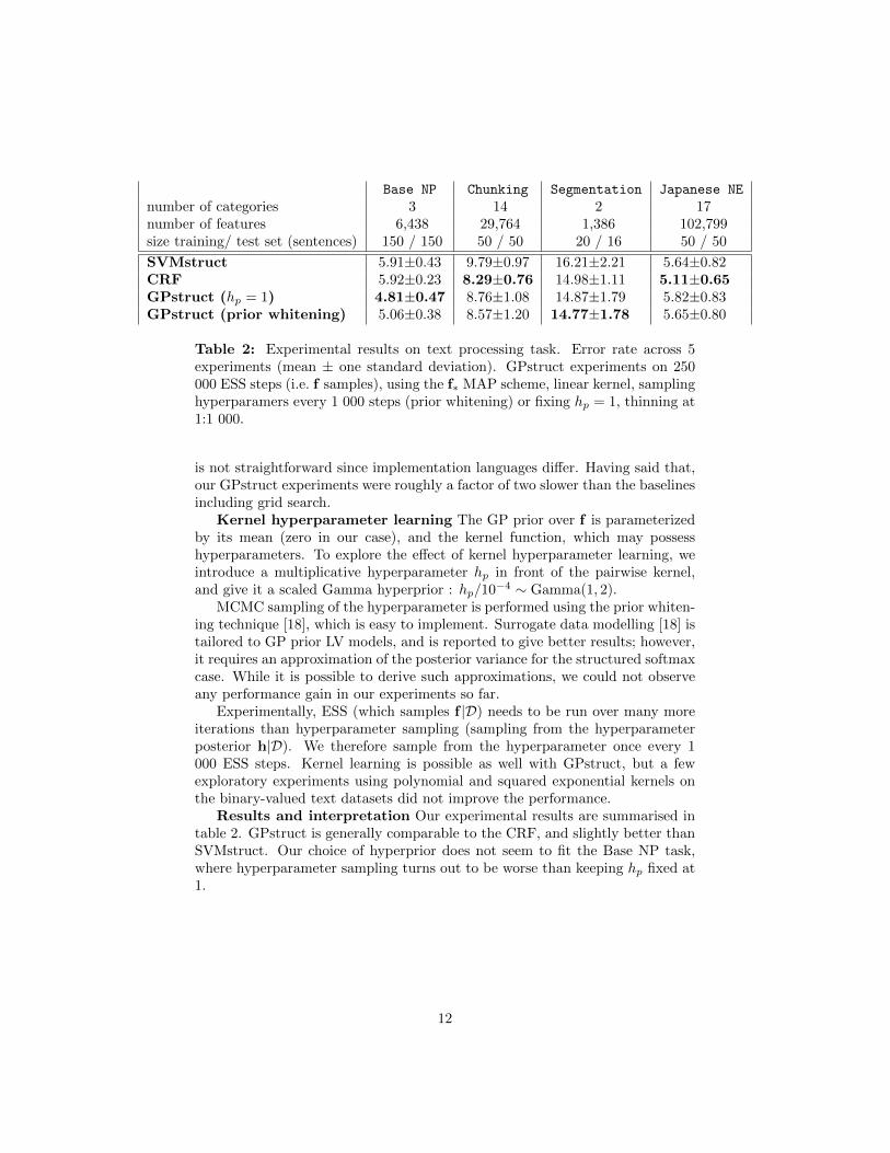
SVMstruct 5.91±0.43 9.79±0.97 16.21±2.21 5.64±0.82CRF 5.92±0.23 8.29±0.76 14.98±1.11 5.11±0.65GPstruct (hp = 1) 4.81±0.47 8.76±1.08 14.87±1.79 5.82±0.83GPstruct (prior whitening) 5.06±0.38 8.57±1.20 14.77±1.78 5.65±0.80

Table 2: Experimental results on text processing task. Error rate across 5experiments (mean ± one standard deviation). GPstruct experiments on 250000 ESS steps (i.e. f samples), using the f∗ MAP scheme, linear kernel, samplinghyperparamers every 1 000 steps (prior whitening) or fixing hp = 1, thinning at1:1 000.

is not straightforward since implementation languages differ. Having said that,our GPstruct experiments were roughly a factor of two slower than the baselinesincluding grid search.

Kernel hyperparameter learning The GP prior over f is parameterizedby its mean (zero in our case), and the kernel function, which may possesshyperparameters. To explore the effect of kernel hyperparameter learning, weintroduce a multiplicative hyperparameter hp in front of the pairwise kernel,and give it a scaled Gamma hyperprior : hp/10−4 ∼ Gamma(1, 2).

MCMC sampling of the hyperparameter is performed using the prior whiten-ing technique [18], which is easy to implement. Surrogate data modelling [18] istailored to GP prior LV models, and is reported to give better results; however,it requires an approximation of the posterior variance for the structured softmaxcase. While it is possible to derive such approximations, we could not observeany performance gain in our experiments so far.

Experimentally, ESS (which samples f |D) needs to be run over many moreiterations than hyperparameter sampling (sampling from the hyperparameterposterior h|D). We therefore sample from the hyperparameter once every 1000 ESS steps. Kernel learning is possible as well with GPstruct, but a fewexploratory experiments using polynomial and squared exponential kernels onthe binary-valued text datasets did not improve the performance.

Results and interpretation Our experimental results are summarised intable 2. GPstruct is generally comparable to the CRF, and slightly better thanSVMstruct. Our choice of hyperprior does not seem to fit the Base NP task,where hyperparameter sampling turns out to be worse than keeping hp fixed at1.

12

20 30 40 50 60 70 80CRF, Error rate

20

30

40

50

60

70

80G

Pst

ruct

SE k

ern

el, E

rror

rate

5 / 20

15 / 20

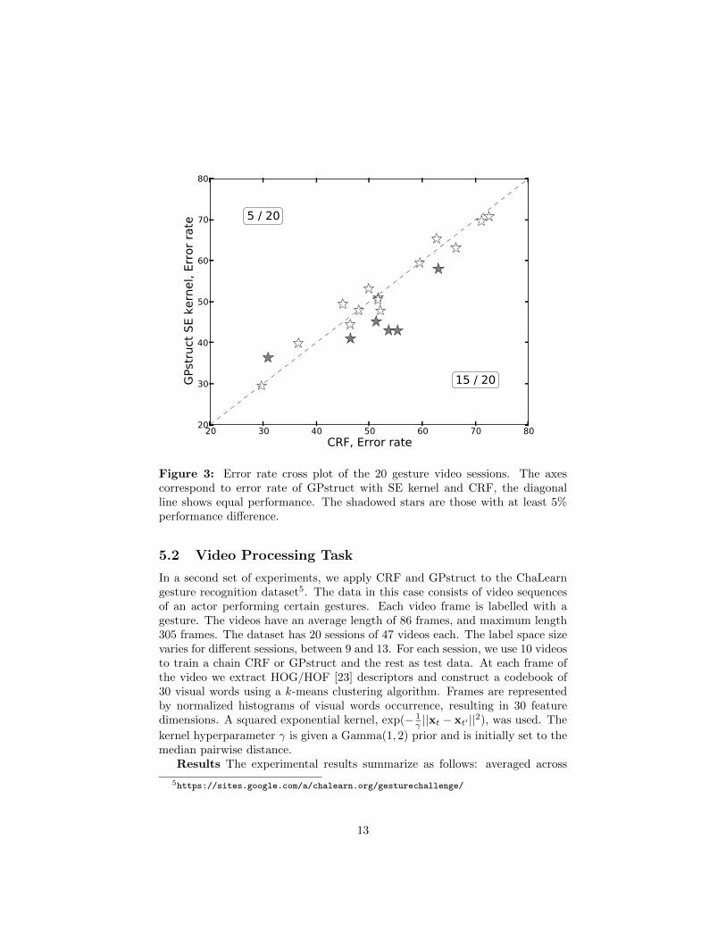
Figure 3: Error rate cross plot of the 20 gesture video sessions. The axescorrespond to error rate of GPstruct with SE kernel and CRF, the diagonalline shows equal performance. The shadowed stars are those with at least 5%performance difference.

5.2 Video Processing Task

In a second set of experiments, we apply CRF and GPstruct to the ChaLearngesture recognition dataset5. The data in this case consists of video sequencesof an actor performing certain gestures. Each video frame is labelled with agesture. The videos have an average length of 86 frames, and maximum length305 frames. The dataset has 20 sessions of 47 videos each. The label space sizevaries for different sessions, between 9 and 13. For each session, we use 10 videosto train a chain CRF or GPstruct and the rest as test data. At each frame ofthe video we extract HOG/HOF [23] descriptors and construct a codebook of30 visual words using a k-means clustering algorithm. Frames are representedby normalized histograms of visual words occurrence, resulting in 30 featuredimensions. A squared exponential kernel, exp(− 1

γ ||xt − xt′ ||2), was used. The

kernel hyperparameter γ is given a Gamma(1, 2) prior and is initially set to themedian pairwise distance.

Results The experimental results summarize as follows: averaged across

5https://sites.google.com/a/chalearn.org/gesturechallenge/

13

all 20 sessions, the error rates were 52.12 ± 11.73 for the CRF, 51.91 ± 11.02for GPstruct linear kernel, and 50.42 ± 11.24 for GPstruct SE kernel. Sinceeach session effectively represents one specific learning task, we compare thepairwise performances across 20 sessions between GPstruct SE kernel and CRFin figure 3. GPstruct outperforms the CRF baseline by more than 5% in fivecases, while it underperforms it in one case. The performance between GPstructlinear kernel and CRF are comparable and we did not include details here dueto space constraints.

5.3 Practical insights

We will open-source our GPstruct code on MLOSS6 to expose the GPstructmodel more widely and encourage experimentation.

Kernel matrix positive-definiteness To preserve numerical stability ofthe Cholesky operation, diagonal jitter of 10−4 is added to the kernel matrices.Depending on the hyperprior, some hyperparameter samples may make thekernel matrices badly conditioned: this is best prevented by rejecting such aproposal by simulating a very low likelihood value.

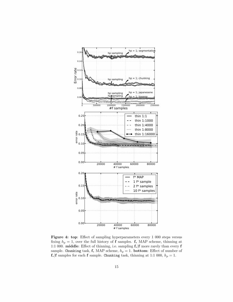
How many f samples? All subplots in figure 4 plot the error rate ofsome configuration against the number of f samples generated (i.e. iterationsof the ESS procedure). For all our tasks, the error rate improves until 100000 iterations, which shows heuristically that sampling histories of at least thislength are needed to attain equilibrium for these problems.

How many f∗|f samples? f∗ need not be sampled for every f samplewhich is generated; to save computing time, we can thin and e.g. sample f∗|fonly every 10th f sample, disregarding the other nine samples entirely. Ourexploratory experiments show the following: high thinning rates, such as 1:4000, seem to have very limited impact on the error rate, cf. figure 4 (middle).Similarly, how many samples f∗|f do we need? Do we need any at all, or could weuse only the mean of the predictive posterior? This would save computing thepredictive variance, which involves a Cholesky matrix inversion, and is called“f∗ MAP” here. Figure 4 (bottom) answers this: sampling more often doesnot decrease the error rate. These findings are very valuable in practice, andseem to indicate that the predictive posterior is peaked, while the posterioris rather flat, and requires a long MCMC exploration path to be adequatelysampled from. Computing time is dictated by the ESS sampling procedure, soperformance improvement efforts should clearly aim at obtaining decorrelatedposterior samples.

6 Conclusions and future work

As a model, GPstruct possesses many desirable properties, discussed in detailabove. Our experiments with sequential data yielded encouraging results: we

6www.mloss.org

14

0 500000 1000000 1500000 2000000 2500000

#f samples

0.06

0.08

0.10

0.12

0.14

0.16

Err

or

rate

hp = 1; chunkinghp sampling

hp = 1; segmentationhp sampling

hp = 1; japanesenehp samplinghp = 1; basenphp sampling

20000 40000 60000 80000# f samples

0.00

0.05

0.10

0.15

0.20

0.25

err

or

rate

thin 1:1thin 1:1000thin 1:4000thin 1:8000thin 1:16000

20000 40000 60000 80000# f samples

0.00

0.05

0.10

0.15

0.20

err

or

rate

f* MAP1 f* sample2 f* samples10 f* samples

Figure 4: top: Effect of sampling hyperparameters every 1 000 steps versusfixing hp = 1, over the full history of f samples. f∗ MAP scheme, thinning at1:1 000. middle: Effect of thinning, i.e. sampling f∗|f more rarely than every fsample. Chunking task, f∗ MAP scheme, hp = 1. bottom: Effect of number off∗|f samples for each f sample. Chunking task, thinning at 1:1 000, hp = 1.

15

achieve performance comparable to CRF and exceed SVMstruct in text pro-cessing tasks, and exceed CRF in a video processing task. While GPstruct istheoretically attractive and empirically promising, we have clearly only touchedthe surface of the model’s possibilities. An important limitation preventing theapplication to larger data sets is the size of the kernel matrix K, square inthe number of LV. One promising direction is an ensemble learning approachin which weak learners can be trained on subsets of the LV constrained bythe underlying MRF (thus with quadratically smaller K), and their predictionscombined, by Bayesian model combination, into a strong learner.

References

[1] Ben Taskar, Carlos Guestrin, and Daphne Koller. Max-margin Markovnetworks. In NIPS, 2004.

[2] Ioannis Tsochantaridis, Thorsten Joachims, Thomas Hofmann, andYasemin Altun. Large margin methods for structured and interdependentoutput variables. JMLR, 6:1453–1484, 2005.

[3] John D. Lafferty, Andrew McCallum, and Fernando C. N. Pereira. Con-ditional random fields: Probabilistic models for segmenting and labelingsequence data. In ICML, 2001.

[4] Carl E. Rasmussen and Christopher K. I. Williams. Gaussian Processesfor Machine Learning. MIT Press, 2006.

[5] Christopher K. I. Williams and David Barber. Bayesian ClassificationWith Gaussian Processes. IEEE Trans. Pattern Anal. Mach. Intelligence,20(12):1342–1351, 1998.

[6] John Lafferty, Xiaojin Zhu, and Yan Liu. Kernel conditional random fields:representation and clique selection. In ICML, 2004.

[7] Yuan Qi, Martin Szummer, and Thomas P. Minka. Bayesian conditionalrandom fields. In AISTATS, 2005.

[8] Yasemin Altun, Thomas Hofmann, and Alexander J. Smola. Gaussianprocess classification for segmenting and annotating sequences. In ICML,2004.

[9] Jason Weston and Chris Watkins. Support vector machines for multi-classpattern recognition. In Proceedings of the Seventh European SymposiumOn Artificial Neural Networks, 1999.

[10] Koby Crammer and Yoram Singer. On the algorithmic implementation ofmulticlass kernel-based vector machines. JMLR, 2:265–292, 2001.

16

[11] Fernando Perez-Cruz, Massimiliano Pontil, and Zoubin Ghahramani. Con-ditional graphical models. In Predicting Structured Data, pages 265–282.MIT Press, 2007.

[12] Charles A. Sutton and Andrew McCallum. An introduction to conditionalrandom fields. Foundations and Trends in Machine Learning, 4(4):267–373,2012.

[13] Sebastian Nowozin and Christoph H. Lampert. Structured learning and pre-diction in computer vision. Foundations and Trends in Computer Graphicsand Vision, 2011.

[14] Ben Taskar, Dan Klein, Michael Collins, Daphne Koller, and ChristopherManning. Max-margin parsing. In Conference on Empirical Methods onNatural Language Processing (EMNLP), 2004.

[15] Bernhard Scholkopf and Alexander J. Smola. Learning with Kernels: Sup-port Vector Machines, Regularization, Optimization, and Beyond. MITPress, 2001.

[16] Kevin P. Murphy, Yair Weiss, and Michael I. Jordan. Loopy belief propa-gation for approximate inference: An empirical study. In UAI, 1999.

[17] Hannes Nickisch. Approximations for Binary Gaussian Process Classifica-tion. JMLR, 2008.

[18] Iain Murray, Ryan P. Adams, and David J. C. MacKay. Elliptical slicesampling. JMLR - Proceedings Track, 9:541–548, 2010.

[19] Jeremy Jancsary, Sebastian Nowozin, Toby Sharp, and Carsten Rother. Re-gression tree fields - an efficient, non-parametric approach to image labelingproblems. In CVPR, 2012.

[20] Thomas P. Minka. A family of algorithms for approximate bayesian infer-ence. PhD thesis, MIT, 2001.

[21] Jason Weston, Olivier Chapelle, Andre Elisseeff, Bernhard Scholkopf, andVladimir Vapnik. Kernel dependency estimation. In NIPS, 2002.

[22] Liefeng Bo and Cristian Sminchisescu. Twin gaussian processes for struc-tured prediction. IJCV, 2010.

[23] Ivan Laptev, Marcin Marszalek, Cordelia Schmid, and Benjamin Rozenfeld.Learning realistic human actions from movies. In CVPR, 2008.

Acknowledgments

The authors would like to thank Simon Lacoste-Julien, Viktoriia Sharmanska,and Chao Chen for discussions.

17