bayesian uncertainty estimation for batch normalized deep ... · bayesian uncertainty estimation...
TRANSCRIPT
Bayesian Uncertainty Estimation for Batch Normalized Deep Networks
Mattias Teye 1 2 * Hossein Azizpour 1 * Kevin Smith 1 3
AbstractWe show that training a deep network using batchnormalization is equivalent to approximate infer-ence in Bayesian models. We further demon-strate that this finding allows us to make mean-ingful estimates of the model uncertainty us-ing conventional architectures, without modifi-cations to the network or the training proce-dure. Our approach is thoroughly validated bymeasuring the quality of uncertainty in a seriesof empirical experiments on different tasks. Itoutperforms baselines with strong statistical sig-nificance, and displays competitive performancewith recent Bayesian approaches.
1. IntroductionDeep learning has dramatically advanced the state of theart in a number of domains. Despite their unprecedenteddiscriminative power, deep networks are prone to makemistakes. Nevertheless, they can already be found in set-tings where errors carry serious repercussions such as au-tonomous vehicles (Chen et al., 2016) and high frequencytrading. We can soon expect automated systems to screenfor various types of cancer (Esteva et al., 2017; Shen, 2017)and diagnose biopsies (Djuric et al., 2017). As autonomoussystems based on deep learning are increasingly deployedin settings with the potential to cause physical or economicharm, we need to develop a better understanding of whenwe can be confident in the estimates produced by deep net-works, and when we should be less certain.
Standard deep learning techniques used for supervisedlearning lack methods to account for uncertainty in themodel. This can be problematic when the network en-counters conditions it was not exposed to during training,
* Co-first authorship 1School of Electrical Engineering andComputer Science, KTH Royal Institute of Technology, Stock-holm, Sweden 2Current address: Electronic Arts, SEED, Stock-holm, Sweden. This work was carried out at Budbee AB.3Science for Life Laboratory. Correspondence to: Kevin Smith<[email protected]>.
Proceedings of the 35 th International Conference on MachineLearning, Stockholm, Sweden, PMLR 80, 2018. Copyright 2018by the author(s).
or if the network is confronted with adversarial examples(Goodfellow et al., 2014). When exposed to data outsidethe distribution it was trained on, the network is forced toextrapolate, which can lead to unpredictable behavior.
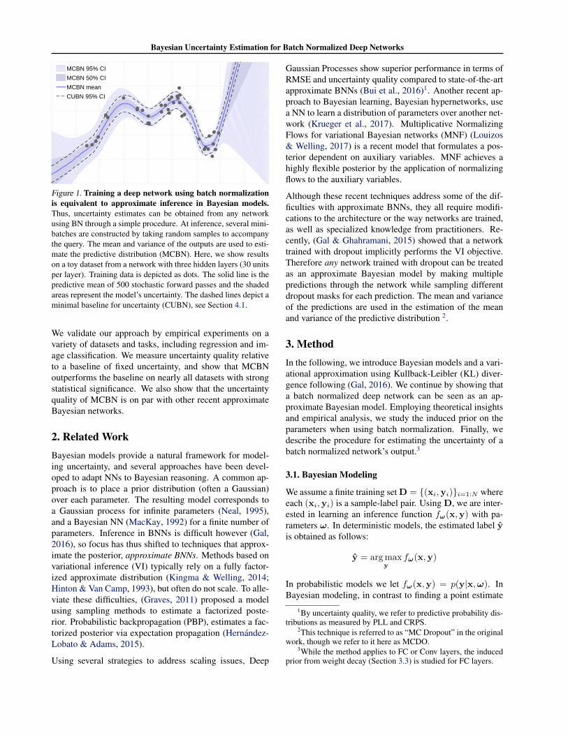
If the network can provide information about its uncer-tainty in addition to its point estimate, disaster may beavoided. In this work, we focus on estimating such pre-dictive uncertainties in deep networks (Figure 1).
The Bayesian approach provides a theoretical frameworkfor modeling uncertainty (Ghahramani, 2015), which hasprompted several attempts to extend neural networks (NN)into a Bayesian setting. Most notably, Bayesian neural net-works (BNNs) have been studied since the 1990’s (Neal,2012), but do not scale well and struggle to compete withmodern deep learning architectures. Recently, (Gal &Ghahramani, 2015) developed a practical solution to obtainuncertainty estimates by casting dropout training in con-ventional deep networks as a Bayesian approximation of aGaussian Process (its correspondence to a general approx-imate Bayesian model was shown in (Gal, 2016)). Theyshowed that any network trained with dropout is an ap-proximate Bayesian model, and uncertainty estimates canbe obtained by computing the variance on multiple predic-tions with different dropout masks.
The inference in this technique, called Monte CarloDropout (MCDO), has an attractive quality: it can be ap-plied to any pre-trained networks with dropout layers. Un-certainty estimates come (nearly) for free. However, not allarchitectures use dropout, and most modern networks haveadopted other regularization techniques. Batch normaliza-tion (BN), in particular, has become widespread thanks toits ability to stabilize learning with improved generalization(Ioffe & Szegedy, 2015).
An interesting aspect of BN is that the mini-batch statis-tics used for training each iteration depend on randomlyselected batch members. We exploit this stochasticity andshow that training using batch normalization, like dropout,can be cast as an approximate Bayesian inference. Wedemonstrate how this finding allows us to make meaning-ful estimates of the model uncertainty in a technique wecall Monte Carlo Batch Normalization (MCBN) (Figure 1).The method we propose can be applied to any network us-ing standard batch normalization.
arX
iv:1
802.
0645
5v2
[st
at.M
L]
16
Jul 2
018
Bayesian Uncertainty Estimation for Batch Normalized Deep Networks
MCBN 95% CI
MCBN 50% CI
MCBN mean
CUBN 95% CI
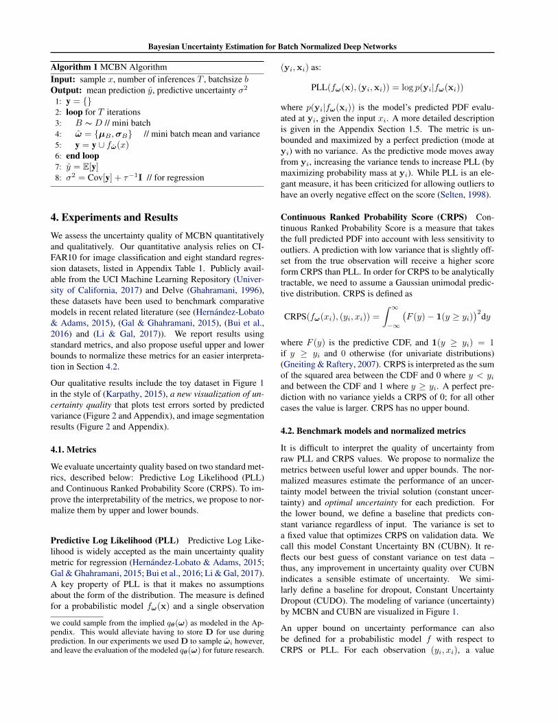
Figure 1. Training a deep network using batch normalizationis equivalent to approximate inference in Bayesian models.Thus, uncertainty estimates can be obtained from any networkusing BN through a simple procedure. At inference, several mini-batches are constructed by taking random samples to accompanythe query. The mean and variance of the outputs are used to esti-mate the predictive distribution (MCBN). Here, we show resultson a toy dataset from a network with three hidden layers (30 unitsper layer). Training data is depicted as dots. The solid line is thepredictive mean of 500 stochastic forward passes and the shadedareas represent the model’s uncertainty. The dashed lines depict aminimal baseline for uncertainty (CUBN), see Section 4.1.
We validate our approach by empirical experiments on avariety of datasets and tasks, including regression and im-age classification. We measure uncertainty quality relativeto a baseline of fixed uncertainty, and show that MCBNoutperforms the baseline on nearly all datasets with strongstatistical significance. We also show that the uncertaintyquality of MCBN is on par with other recent approximateBayesian networks.
2. Related WorkBayesian models provide a natural framework for model-ing uncertainty, and several approaches have been devel-oped to adapt NNs to Bayesian reasoning. A common ap-proach is to place a prior distribution (often a Gaussian)over each parameter. The resulting model corresponds toa Gaussian process for infinite parameters (Neal, 1995),and a Bayesian NN (MacKay, 1992) for a finite number ofparameters. Inference in BNNs is difficult however (Gal,2016), so focus has thus shifted to techniques that approx-imate the posterior, approximate BNNs. Methods based onvariational inference (VI) typically rely on a fully factor-ized approximate distribution (Kingma & Welling, 2014;Hinton & Van Camp, 1993), but often do not scale. To alle-viate these difficulties, (Graves, 2011) proposed a modelusing sampling methods to estimate a factorized poste-rior. Probabilistic backpropagation (PBP), estimates a fac-torized posterior via expectation propagation (Hernandez-Lobato & Adams, 2015).
Using several strategies to address scaling issues, Deep
Gaussian Processes show superior performance in terms ofRMSE and uncertainty quality compared to state-of-the-artapproximate BNNs (Bui et al., 2016)1. Another recent ap-proach to Bayesian learning, Bayesian hypernetworks, usea NN to learn a distribution of parameters over another net-work (Krueger et al., 2017). Multiplicative NormalizingFlows for variational Bayesian networks (MNF) (Louizos& Welling, 2017) is a recent model that formulates a pos-terior dependent on auxiliary variables. MNF achieves ahighly flexible posterior by the application of normalizingflows to the auxiliary variables.
Although these recent techniques address some of the dif-ficulties with approximate BNNs, they all require modifi-cations to the architecture or the way networks are trained,as well as specialized knowledge from practitioners. Re-cently, (Gal & Ghahramani, 2015) showed that a networktrained with dropout implicitly performs the VI objective.Therefore any network trained with dropout can be treatedas an approximate Bayesian model by making multiplepredictions through the network while sampling differentdropout masks for each prediction. The mean and varianceof the predictions are used in the estimation of the meanand variance of the predictive distribution 2.
3. MethodIn the following, we introduce Bayesian models and a vari-ational approximation using Kullback-Leibler (KL) diver-gence following (Gal, 2016). We continue by showing thata batch normalized deep network can be seen as an ap-proximate Bayesian model. Employing theoretical insightsand empirical analysis, we study the induced prior on theparameters when using batch normalization. Finally, wedescribe the procedure for estimating the uncertainty of abatch normalized network’s output.3
3.1. Bayesian Modeling
We assume a finite training set D = (xi,yi)i=1:N whereeach (xi,yi) is a sample-label pair. Using D, we are inter-ested in learning an inference function fω(x,y) with pa-rameters ω. In deterministic models, the estimated label yis obtained as follows:
y = arg maxy
fω(x,y)
In probabilistic models we let fω(x,y) = p(y|x,ω). InBayesian modeling, in contrast to finding a point estimate
1By uncertainty quality, we refer to predictive probability dis-tributions as measured by PLL and CRPS.
2This technique is referred to as “MC Dropout” in the originalwork, though we refer to it here as MCDO.
3While the method applies to FC or Conv layers, the inducedprior from weight decay (Section 3.3) is studied for FC layers.
Bayesian Uncertainty Estimation for Batch Normalized Deep Networks
of the model parameters, the idea is to estimate an (ap-proximate) posterior distribution of the model parametersp(ω|D) to be used for probabilistic prediction:
p(y|x,D) =
∫fω(x,y)p(ω|D)dω
The predicted label, y, can then be accordingly obtained bysampling p(y|x,D) or taking its maxima.
Variational Approximation In approximate Bayesianmodeling, a common approach is to learn a parame-terized approximating distribution qθ(ω) that minimizesKL(qθ(ω)||p(ω|D)); the Kullback-Leibler divergence ofthe true posterior w.r.t. its approximation. Minimizing thisKL divergence is equivalent to the following minimizationwhile being free of the data term p(D) 4:
LVA(θ) :=−N∑i=1
∫qθ(ω) ln fω(xi,yi)dω
+ KL(qθ(ω)||p(ω))
During optimization, we want to take the derivative of theexpected likelihood w.r.t. the learnable parameters θ. Weuse the same MC estimate as in (Gal, 2016) (explained inAppendix Section 1.1), such that one realized ωi is takenfor each sample i 5. Optimizing over mini-batches of sizeM , the approximated objective becomes:
LVA(θ) := −NM
M∑i=1
ln fωi(xi,yi) + KL(qθ(ω)||p(ω)) (1)
The first term is the data likelihood and the second termis the divergence of the prior w.r.t. the approximated poste-rior.
3.2. Batch Normalized Deep Nets as Bayesian Modeling
We now describe the optimization procedure of a deep net-work with batch normalization and draw the resemblanceto the approximate Bayesian modeling in Eq (1).
The inference function of a feed-forward deep networkwith L layers can be described as:
fω(x) = WLa(WL−1...a(W2a(W1x))
4Achieved by constructing the Evidence Lower Bound, calledELBO, and assuming i.i.d. observation noise; details can be foundin Appendix Section 1.1.
5While a MC integration using a single sample is a weak ap-proximation, in an iterative optimization for θ several sampleswill be taken over time.
where a(.) is an element-wise nonlinearity function andWl is the weight vector at layer l. Furthermore, we de-note the input to layer l as xl with x1 = x and we then sethl = Wlxl. Parenthesized super-index for matrices (e.g.W(j)) and vectors (e.g. x(j)) indicates jth row and elementrespectively. Super-index u refers to a specific unit at layerl, (e.g. Wu = Wl,(j), hu = hl,(j)). 6
Batch Normalization Each layer of a deep network isconstructed by several linear units whose parameters arethe rows of the weight matrix W. Batch normalization isa unit-wise operation proposed in (Ioffe & Szegedy, 2015)to standardize the distribution of each unit’s input. For FClayers, it converts a unit’s input hu in the following way:
hu =hu − E[hu]√
Var[hu]
where the expectations are computed over the trainingset during evaluation, and mini-batch during training (indeep networks, the weight matrices are often optimized us-ing back-propagated errors calculated on mini-batches ofdata)7. Therefore, during training, the estimated mean andvariance on the mini-batch B is used, which we denote byµB and σB respectively. This makes the inference at train-ing time for a sample x a stochastic process, varying basedon other samples in the mini-batch.
Loss Function and Optimization Training deep net-works with mini-batch optimization involves a (regular-ized) risk minimization with the following form:
LRR(ω) :=1
M
M∑i=1
l(yi,yi) + Ω(ω)
where the first term is the empirical loss on the trainingdata and the second term is a regularization penalty act-ing as a prior on model parameters ω. If the loss l iscross-entropy for classification or sum-of-squares for re-gression problems (assuming i.i.d. Gaussian noise on la-bels), the first term is equivalent to minimizing the negativelog-likelihood:
LRR(ω) := − 1
Mτ
M∑i=1
ln fω(xi,yi) + Ω(ω)
6For a (softmax) classification network, fω(x) is a vector withfω(x,y) = fω(x)(y), for regression networks with i.i.d. Gaus-sian noise we have fω(x,y) = N (fω(x), τ−1I).
7It also learns an affine transformation for each unit with pa-rameters γ and β, omitted for brevity: x(j)affine = γ(j)x(j) + β(j).
Bayesian Uncertainty Estimation for Batch Normalized Deep Networks
with τ = 1 for classification. In a networkwith batch normalization, the model parameters includeW1:L,γ1:L,β1:L,µ1:L
B ,σ1:LB . If we decouple the learn-
able parameters θ = W1:L,γ1:L,β1:L from the stochas-tic parameters ω = µ1:L
B ,σ1:LB , we get the following ob-
jective at each step of the mini-batch optimization:
LRR(θ) := − 1
Mτ
M∑i=1
ln fθ,ωi(xi,yi) + Ω(θ) (2)
where ωi is the means and variances for sample i’s mini-batch at a certain training step. Note that while ωi formallyneeds to be i.i.d. for each training example, a batch normal-ized network samples the stochastic parameters once pertraining step (mini-batch). For a large number of epochs,however, the distribution of sampled batch members for agiven training example converges to the i.i.d. case.
In a batch normalized network, qθ(ω) corresponds to thejoint distribution of the weights, induced by the random-ness of the normalization parameters µ1:L
B ,σ1:LB , as im-
plied by the repeated sampling from D during training.This is an approximation of the true posterior, where wehave restricted the posterior to lie within the domain ofour parametric network and source of randomness. Withthat, we can estimate the uncertainty of predictions froma trained batch normalized network using the inherentstochasticity of BN (Section 3.4).
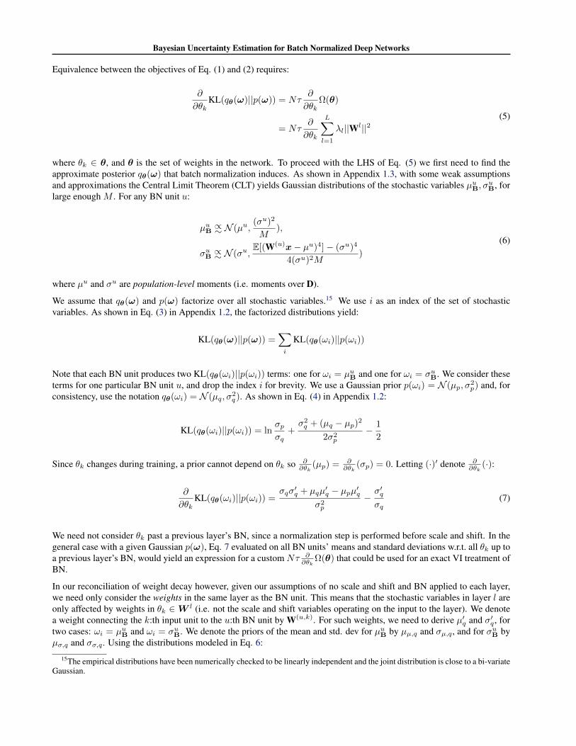
3.3. Prior p(ω)
Equivalence between the VA and BN training proceduresrequires ∂
∂θ of Eq. (1) and Eq. (2) to be equivalent up to ascaling factor. This is the case if ∂
∂θKL(qθ(ω)||p(ω)) =
Nτ ∂∂θΩ(θ).
To reconcile this condition, one option is to let the priorp(ω) imply the regularization term Ω(θ). Eq. (1) revealsthat the contribution of KL(qθ(ω)||p(ω)) to the optimiza-tion objective is inversely scaled with N . For BN, this cor-responds to a model with a small Ω(θ) when N is large. Inthe limit as N →∞, the optimization objectives of Eq. (1)and Eq. (2) become identical with no regularization.8
Another option is to let some Ω(θ) imply p(ω). In Ap-pendix Section 1.4 we explore this with L2-regularization,also called weight decay (Ω(θ) = λ
∑l=1:L ||W l||2). We
find that unlike in MCDO (Gal, 2016), some simplifying
8To prove the existence and find an expression ofKL(qθ(ω)||p(ω)), in Appendix Section 1.3 we find that BN ap-proximately induces Gaussian distributions over BN units’ meansand standard deviations, centered around the population valuesgiven by D. We assume a factorized distribution and Gaussianpriors, and find the corresponding KL(qθ(ω)||p(ω)) componentsin Appendix Section 1.4 Eq. (7). These could be used to constructa custom Ω(θ) for any Gaussian choice of p(ω).
assumptions are necessary to reconcile the VA and BN ob-jectives with weight decay: no scale and shift applied toBN layers, uncorrelated units in each layer, BN applied onall layers, and large N and M . Given these conditions:
p(µuB) = N (µµ,p, σµ,p)
p(σuB) = N (µσ,p, σσ,p)
where µµ,p = 0, σµ,p →∞, µσ,p = 0 and σσ,p → 12Nτλl
.
This corresponds to a wide and narrow distribution on BNunits’ means and std. devs respectively, where N accountsfor the narrowness of the prior. Due to its popularity indeep learning, our experiments in Section 4 are performedwith weight decay.
3.4. Predictive Uncertainty in Batch Normalized DeepNets
In the absence of the true posterior, we rely on the approx-imate posterior to express an approximate predictive distri-bution:
p∗(y|x,D) :=
∫fω(x,y)qθ(ω)dω
Following (Gal, 2016) we estimate the first (for regressionand classification) and second (for regression) moments ofthe predictive distribution empirically (see Appendix Sec-tion 1.5 for details):
Ep∗ [y] ≈ 1
T
T∑i=1
fωi(x)
Covp∗ [y] ≈ τ−1I +1
T
T∑i=1
fωi(x)ᵀfωi
(x)
− Ep∗ [y]ᵀEp∗ [y]
where each ωi corresponds to sampling the net’s stochas-tic parameters ω = µ1:L
B ,σ1:LB the same way as during
training. Sampling ωi therefore involves sampling a batchB from the training set and updating the parameters in theBN units, just as if we were taking a training step with B.From a VA perspective, training the network amounted tominimizing KL(qθ(ω)||p(ω|D)) wrt θ. Sampling ωi fromthe training set, and keeping the size of B consistent withthe mini-batch size used during training, ensures that qθ(ω)during inference remains identical to the approximate pos-terior optimized during training.
The network is trained just as a regular BN network, butinstead of replacing ω = µ1:L
B ,σ1:LB with population
values from D for inference, we update these parametersstochastically, once for each forward pass.9 Pseudocodefor estimating predictive mean and variance is given in Al-gorithm 1.
9As an alternative to using the training set D to sample ωi,
Bayesian Uncertainty Estimation for Batch Normalized Deep Networks
Algorithm 1 MCBN AlgorithmInput: sample x, number of inferences T , batchsize bOutput: mean prediction y, predictive uncertainty σ2
1: y = 2: loop for T iterations3: B ∼ D // mini batch4: ω = µB ,σB // mini batch mean and variance5: y = y ∪ fω(x)6: end loop7: y = E[y]8: σ2 = Cov[y] + τ−1I // for regression
4. Experiments and ResultsWe assess the uncertainty quality of MCBN quantitativelyand qualitatively. Our quantitative analysis relies on CI-FAR10 for image classification and eight standard regres-sion datasets, listed in Appendix Table 1. Publicly avail-able from the UCI Machine Learning Repository (Univer-sity of California, 2017) and Delve (Ghahramani, 1996),these datasets have been used to benchmark comparativemodels in recent related literature (see (Hernandez-Lobato& Adams, 2015), (Gal & Ghahramani, 2015), (Bui et al.,2016) and (Li & Gal, 2017)). We report results usingstandard metrics, and also propose useful upper and lowerbounds to normalize these metrics for an easier interpreta-tion in Section 4.2.
Our qualitative results include the toy dataset in Figure 1in the style of (Karpathy, 2015), a new visualization of un-certainty quality that plots test errors sorted by predictedvariance (Figure 2 and Appendix), and image segmentationresults (Figure 2 and Appendix).
4.1. Metrics
We evaluate uncertainty quality based on two standard met-rics, described below: Predictive Log Likelihood (PLL)and Continuous Ranked Probability Score (CRPS). To im-prove the interpretability of the metrics, we propose to nor-malize them by upper and lower bounds.
Predictive Log Likelihood (PLL) Predictive Log Like-lihood is widely accepted as the main uncertainty qualitymetric for regression (Hernandez-Lobato & Adams, 2015;Gal & Ghahramani, 2015; Bui et al., 2016; Li & Gal, 2017).A key property of PLL is that it makes no assumptionsabout the form of the distribution. The measure is definedfor a probabilistic model fω(x) and a single observation
we could sample from the implied qθ(ω) as modeled in the Ap-pendix. This would alleviate having to store D for use duringprediction. In our experiments we used D to sample ωi however,and leave the evaluation of the modeled qθ(ω) for future research.
(yi,xi) as:
PLL(fω(x), (yi,xi)) = log p(yi|fω(xi))
where p(yi|fω(xi)) is the model’s predicted PDF evalu-ated at yi, given the input xi. A more detailed descriptionis given in the Appendix Section 1.5. The metric is un-bounded and maximized by a perfect prediction (mode atyi) with no variance. As the predictive mode moves awayfrom yi, increasing the variance tends to increase PLL (bymaximizing probability mass at yi). While PLL is an ele-gant measure, it has been criticized for allowing outliers tohave an overly negative effect on the score (Selten, 1998).
Continuous Ranked Probability Score (CRPS) Con-tinuous Ranked Probability Score is a measure that takesthe full predicted PDF into account with less sensitivity tooutliers. A prediction with low variance that is slightly off-set from the true observation will receive a higher scoreform CRPS than PLL. In order for CRPS to be analyticallytractable, we need to assume a Gaussian unimodal predic-tive distribution. CRPS is defined as
CRPS(fω(xi), (yi, xi)) =
∫ ∞−∞
(F (y)− 1(y ≥ yi)
)2dy
where F (y) is the predictive CDF, and 1(y ≥ yi) = 1if y ≥ yi and 0 otherwise (for univariate distributions)(Gneiting & Raftery, 2007). CRPS is interpreted as the sumof the squared area between the CDF and 0 where y < yiand between the CDF and 1 where y ≥ yi. A perfect pre-diction with no variance yields a CRPS of 0; for all othercases the value is larger. CRPS has no upper bound.
4.2. Benchmark models and normalized metrics
It is difficult to interpret the quality of uncertainty fromraw PLL and CRPS values. We propose to normalize themetrics between useful lower and upper bounds. The nor-malized measures estimate the performance of an uncer-tainty model between the trivial solution (constant uncer-tainty) and optimal uncertainty for each prediction. Forthe lower bound, we define a baseline that predicts con-stant variance regardless of input. The variance is set toa fixed value that optimizes CRPS on validation data. Wecall this model Constant Uncertainty BN (CUBN). It re-flects our best guess of constant variance on test data –thus, any improvement in uncertainty quality over CUBNindicates a sensible estimate of uncertainty. We simi-larly define a baseline for dropout, Constant UncertaintyDropout (CUDO). The modeling of variance (uncertainty)by MCBN and CUBN are visualized in Figure 1.
An upper bound on uncertainty performance can alsobe defined for a probabilistic model f with respect toCRPS or PLL. For each observation (yi, xi), a value
Bayesian Uncertainty Estimation for Batch Normalized Deep Networks
for the predictive variance Ti can be chosen that max-imizes PLL or minimizes CRPS10. Using CUBN as alower bound and the optimized CRPS score as the up-per bound, uncertainty estimates can be normalized be-tween these bounds (1 indicating optimal performance,and 0 indicating same performance as fixed uncer-tainty). We call this normalized measure CRPS =
CRPS(f,(yi,xi))−CRPS(fCU ,(yi,xi))minT CRPS(f,(yi,xi))−CRPS(fCU ,(yi,xi))
× 100, and the PLL
analogue PLL = PLL(f,(yi,xi))−PLL(fCU ,(yi,xi))maxT PLL(f,(yi,xi))−PLL(fCU ,(yi,xi))
×100.
4.3. Test setup
Our evaluation compares MCBN to MCDO (Gal &Ghahramani, 2015) and MNF (Louizos & Welling, 2017)using the datasets and metrics described above. Our setupis similar to (Hernandez-Lobato & Adams, 2015), whichwas also followed by (Gal & Ghahramani, 2015). How-ever, our comparison implements a different hyperparame-ter selection, allows for a larger range of dropout rates, anduses larger networks with two hidden layers.
For the regression task, all models share a similar archi-tecture: two hidden layers with 50 units each, and ReLUactivations, with the exception of Protein Tertiary Struc-ture dataset (100 units per hidden layer). Inputs and out-puts were normalized during training. Results were aver-aged over five random splits of 20% test and 80% train-ing and cross-validation (CV) data. For each split, 5-foldCV by grid search with a RMSE minimization objectivewas used to find training hyperparameters and optimal n.o.epochs, out of a maximum of 2000. For BN-based mod-els, the hyperparameter grid consisted of a weight decayfactor ranging from 0.1 to 1−15 by a log 10 scale, and abatch size range from 32 to 1024 by a log 2 scale. ForDO-based models, the hyperparameter grid consisted ofthe same weight decay range, and dropout probabilitiesin 0.2, 0.1, 0.05, 0.01, 0.005, 0.001. DO-based modelsused a batch size of 32 in all evaluations. For MNF11, then.o. epochs was optimized, the batch size was set to 100,and early stopping test performed each epoch (compared toevery 20th for MCBN, MCDO).
For MCBN and MCDO, the model with optimal traininghyperparameters was used to optimize τ numerically. Thisoptimization was made in terms of average CV CRPS forMCBN, CUBN, MCDO, and CUDO respectively.
Estimates for the predictive distribution were obtained bytaking T = 500 stochastic forward passes through the net-work. For each split, test set evaluation was done 5 timeswith different seeds. Implementation was done in Tensor-Flow with the Adam optimizer and a learning rate of 0.001.
10Ti can be found analytically for PLL, but must be found nu-merically for CRPS.
11Where we used an adapted version of the authors’ code.
For the image classification test we use CIFAR10(Krizhevsky & Hinton, 2009) which includes 10 objectclasses with 5,000 and 1,000 images in the training andtest sets, respectively. Images are 32x32 RGB format. Wetrained a ResNet32 architecture with a batch size of 32,learning rate of 0.1, weight decay of 0.0002, leaky ReLUslope of 0.1, and 5 residual units. SGD with momentumwas used as the optimizer.
Code for reproducing our experiments is available athttps://github.com/icml-mcbn/mcbn.
4.4. Test results
The regression experiment comparing uncertainty qualityis summarized in Table 1. We report CRPS and PLL, ex-pressed as a percentage, which reflects how close the modelis to the upper bound, and check to see if the model signif-icantly exceeds the lower bound using a one sample t-test(significance level is indicated by *’s). Further details areprovided in Appendix Section 1.7.
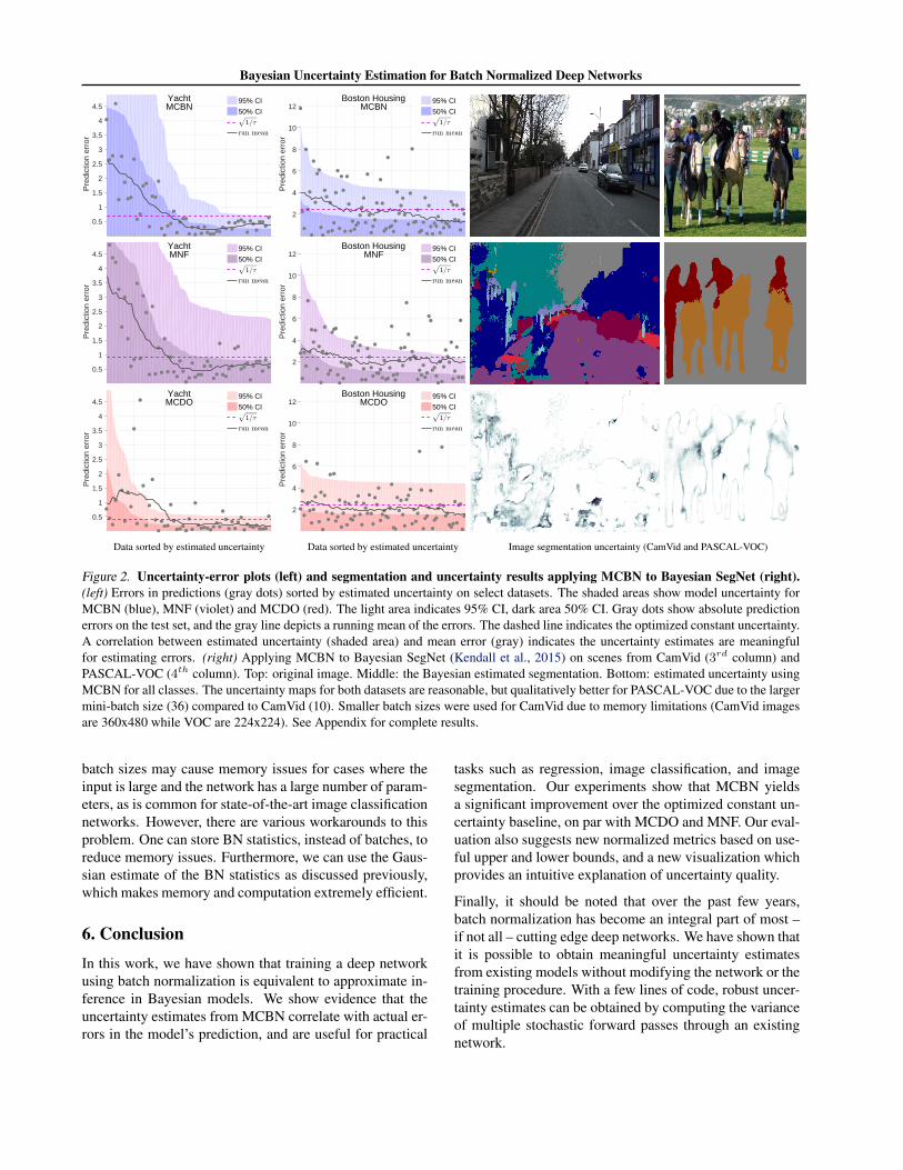
In Figure 2 (left), we present a novel visualization of un-certainty quality for regression problems. Data are sortedby estimated uncertainty in the x-axis. Grey dots show theerrors in model predictions, and the shaded areas show themodel uncertainty. A running mean of the errors appearsas a gray line. If uncertainty estimation is working well,a correlation should exist between the mean error (grayline) and uncertainty (shaded area). This indicates that theuncertainty estimation recognizes samples with larger (orsmaller) potential for predictive errors.
We applied MCBN on the image classification task of CI-FAR10. The baseline in this case is the softmax distribu-tion using the moving average for BN units. Log likeli-hood (PLL) is the metric used to compare with the base-line. The baseline achieves a PLL of -0.32 on the testset, while MCBN obtains a PLL of -0.28. Table 2 showsthe performance of MCBN when using different number ofstochastic forward passes (the MCBN batchsize is fixed tothe training batch size at 32). PLL improves as the numberof the stochastic passes increases, until it is significantlybetter than the softmax baseline.
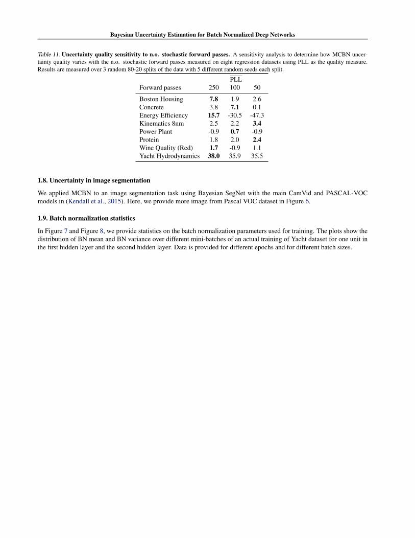
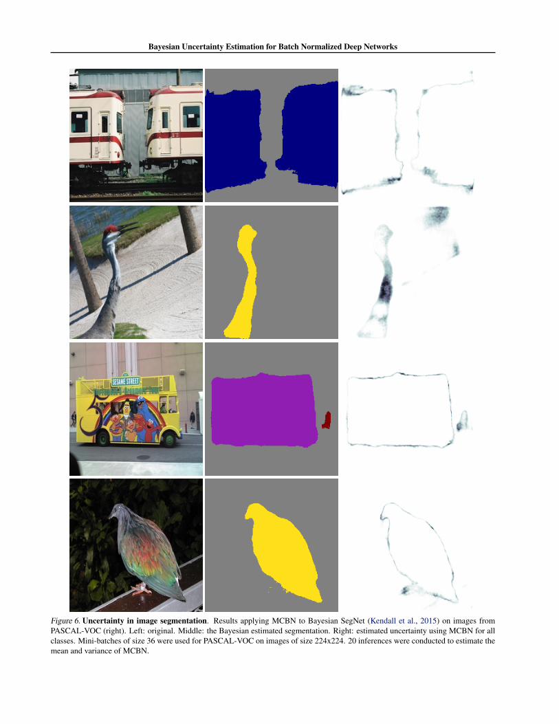
To demonstrate how model uncertainty can be obtainedfrom an existing network with minimal effort, we appliedMCBN to an image segmentation task using Bayesian Seg-Net with the main CamVid and PASCAL-VOC models in(Kendall et al., 2015). We simply ran multiple forwardpasses with different mini-batches randomly taken from thetrain set. The models obtained from the online model zoohave BN blocks after each layer. We recalculate mean andvariance for the first 2 blocks only and use the trainingstatistics for the rest of the blocks. Mini-batches of size10 and 36 were used for CamVid and VOC respectively
Bayesian Uncertainty Estimation for Batch Normalized Deep Networks
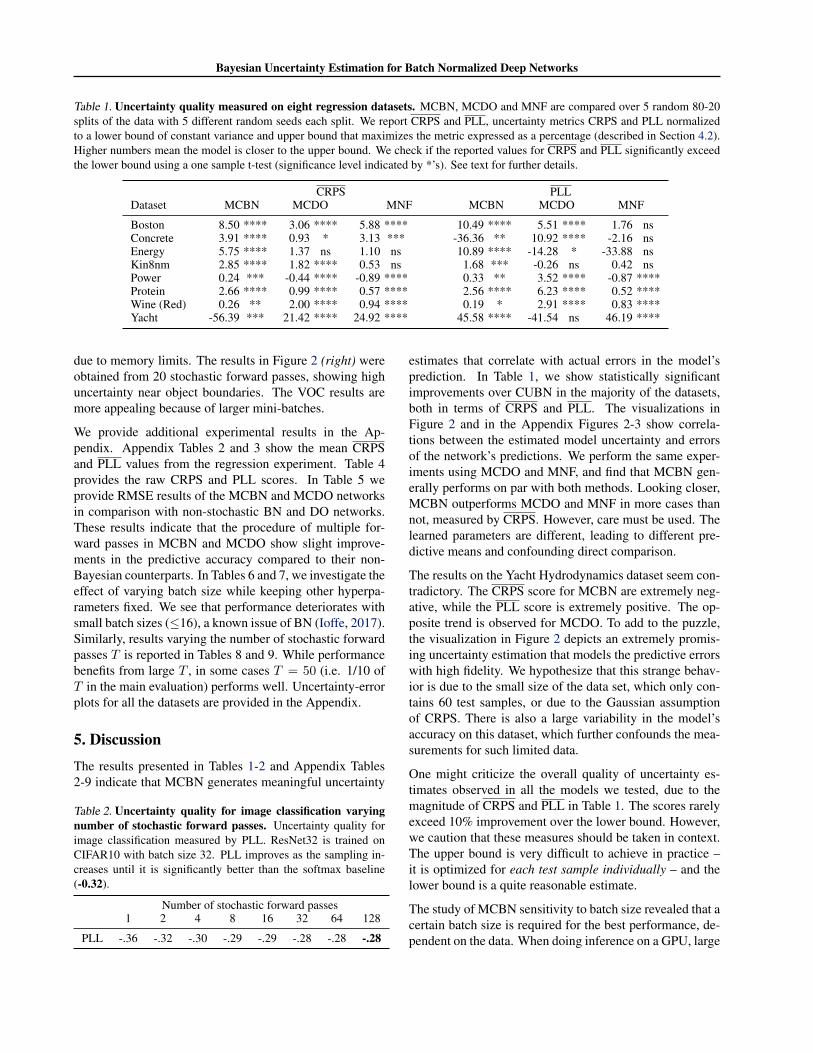
Table 1. Uncertainty quality measured on eight regression datasets. MCBN, MCDO and MNF are compared over 5 random 80-20splits of the data with 5 different random seeds each split. We report CRPS and PLL, uncertainty metrics CRPS and PLL normalizedto a lower bound of constant variance and upper bound that maximizes the metric expressed as a percentage (described in Section 4.2).Higher numbers mean the model is closer to the upper bound. We check if the reported values for CRPS and PLL significantly exceedthe lower bound using a one sample t-test (significance level indicated by *’s). See text for further details.
CRPS PLLDataset MCBN MCDO MNF MCBN MCDO MNF
Boston 8.50 **** 3.06 **** 5.88 **** 10.49 **** 5.51 **** 1.76 nsConcrete 3.91 **** 0.93 * 3.13 *** -36.36 ** 10.92 **** -2.16 nsEnergy 5.75 **** 1.37 ns 1.10 ns 10.89 **** -14.28 * -33.88 nsKin8nm 2.85 **** 1.82 **** 0.53 ns 1.68 *** -0.26 ns 0.42 nsPower 0.24 *** -0.44 **** -0.89 **** 0.33 ** 3.52 **** -0.87 ****Protein 2.66 **** 0.99 **** 0.57 **** 2.56 **** 6.23 **** 0.52 ****Wine (Red) 0.26 ** 2.00 **** 0.94 **** 0.19 * 2.91 **** 0.83 ****Yacht -56.39 *** 21.42 **** 24.92 **** 45.58 **** -41.54 ns 46.19 ****
due to memory limits. The results in Figure 2 (right) wereobtained from 20 stochastic forward passes, showing highuncertainty near object boundaries. The VOC results aremore appealing because of larger mini-batches.
We provide additional experimental results in the Ap-pendix. Appendix Tables 2 and 3 show the mean CRPSand PLL values from the regression experiment. Table 4provides the raw CRPS and PLL scores. In Table 5 weprovide RMSE results of the MCBN and MCDO networksin comparison with non-stochastic BN and DO networks.These results indicate that the procedure of multiple for-ward passes in MCBN and MCDO show slight improve-ments in the predictive accuracy compared to their non-Bayesian counterparts. In Tables 6 and 7, we investigate theeffect of varying batch size while keeping other hyperpa-rameters fixed. We see that performance deteriorates withsmall batch sizes (≤16), a known issue of BN (Ioffe, 2017).Similarly, results varying the number of stochastic forwardpasses T is reported in Tables 8 and 9. While performancebenefits from large T , in some cases T = 50 (i.e. 1/10 ofT in the main evaluation) performs well. Uncertainty-errorplots for all the datasets are provided in the Appendix.
5. DiscussionThe results presented in Tables 1-2 and Appendix Tables2-9 indicate that MCBN generates meaningful uncertainty
Table 2. Uncertainty quality for image classification varyingnumber of stochastic forward passes. Uncertainty quality forimage classification measured by PLL. ResNet32 is trained onCIFAR10 with batch size 32. PLL improves as the sampling in-creases until it is significantly better than the softmax baseline(-0.32).
Number of stochastic forward passes1 2 4 8 16 32 64 128
PLL -.36 -.32 -.30 -.29 -.29 -.28 -.28 -.28
estimates that correlate with actual errors in the model’sprediction. In Table 1, we show statistically significantimprovements over CUBN in the majority of the datasets,both in terms of CRPS and PLL. The visualizations inFigure 2 and in the Appendix Figures 2-3 show correla-tions between the estimated model uncertainty and errorsof the network’s predictions. We perform the same exper-iments using MCDO and MNF, and find that MCBN gen-erally performs on par with both methods. Looking closer,MCBN outperforms MCDO and MNF in more cases thannot, measured by CRPS. However, care must be used. Thelearned parameters are different, leading to different pre-dictive means and confounding direct comparison.
The results on the Yacht Hydrodynamics dataset seem con-tradictory. The CRPS score for MCBN are extremely neg-ative, while the PLL score is extremely positive. The op-posite trend is observed for MCDO. To add to the puzzle,the visualization in Figure 2 depicts an extremely promis-ing uncertainty estimation that models the predictive errorswith high fidelity. We hypothesize that this strange behav-ior is due to the small size of the data set, which only con-tains 60 test samples, or due to the Gaussian assumptionof CRPS. There is also a large variability in the model’saccuracy on this dataset, which further confounds the mea-surements for such limited data.
One might criticize the overall quality of uncertainty es-timates observed in all the models we tested, due to themagnitude of CRPS and PLL in Table 1. The scores rarelyexceed 10% improvement over the lower bound. However,we caution that these measures should be taken in context.The upper bound is very difficult to achieve in practice –it is optimized for each test sample individually – and thelower bound is a quite reasonable estimate.
The study of MCBN sensitivity to batch size revealed that acertain batch size is required for the best performance, de-pendent on the data. When doing inference on a GPU, large
Bayesian Uncertainty Estimation for Batch Normalized Deep Networks
0.5
1
1.5
2
2.5
3
3.5
4
4.5
Pre
dict
ion
erro
r
YachtMCBN
95% CI
50% CI
2
4
6
8
10
12
Pre
dict
ion
erro
r
Boston HousingMCBN
95% CI
50% CI
0.5
1
1.5
2
2.5
3
3.5
4
4.5
Pre
dict
ion
erro
r
YachtMNF
95% CI
50% CI
2
4
6
8
10
12
Pre
dict
ion
erro
r
Boston HousingMNF
95% CI
50% CI
0.5
1
1.5
2
2.5
3
3.5
4
4.5
Pre
dict
ion
erro
r
YachtMCDO
95% CI
50% CI
2
4
6
8
10
12
Pre
dict
ion
erro
r
Boston HousingMCDO
95% CI
50% CI
Data sorted by estimated uncertainty Data sorted by estimated uncertainty Image segmentation uncertainty (CamVid and PASCAL-VOC)
Figure 2. Uncertainty-error plots (left) and segmentation and uncertainty results applying MCBN to Bayesian SegNet (right).(left) Errors in predictions (gray dots) sorted by estimated uncertainty on select datasets. The shaded areas show model uncertainty forMCBN (blue), MNF (violet) and MCDO (red). The light area indicates 95% CI, dark area 50% CI. Gray dots show absolute predictionerrors on the test set, and the gray line depicts a running mean of the errors. The dashed line indicates the optimized constant uncertainty.A correlation between estimated uncertainty (shaded area) and mean error (gray) indicates the uncertainty estimates are meaningfulfor estimating errors. (right) Applying MCBN to Bayesian SegNet (Kendall et al., 2015) on scenes from CamVid (3rd column) andPASCAL-VOC (4th column). Top: original image. Middle: the Bayesian estimated segmentation. Bottom: estimated uncertainty usingMCBN for all classes. The uncertainty maps for both datasets are reasonable, but qualitatively better for PASCAL-VOC due to the largermini-batch size (36) compared to CamVid (10). Smaller batch sizes were used for CamVid due to memory limitations (CamVid imagesare 360x480 while VOC are 224x224). See Appendix for complete results.
batch sizes may cause memory issues for cases where theinput is large and the network has a large number of param-eters, as is common for state-of-the-art image classificationnetworks. However, there are various workarounds to thisproblem. One can store BN statistics, instead of batches, toreduce memory issues. Furthermore, we can use the Gaus-sian estimate of the BN statistics as discussed previously,which makes memory and computation extremely efficient.
6. ConclusionIn this work, we have shown that training a deep networkusing batch normalization is equivalent to approximate in-ference in Bayesian models. We show evidence that theuncertainty estimates from MCBN correlate with actual er-rors in the model’s prediction, and are useful for practical
tasks such as regression, image classification, and imagesegmentation. Our experiments show that MCBN yieldsa significant improvement over the optimized constant un-certainty baseline, on par with MCDO and MNF. Our eval-uation also suggests new normalized metrics based on use-ful upper and lower bounds, and a new visualization whichprovides an intuitive explanation of uncertainty quality.
Finally, it should be noted that over the past few years,batch normalization has become an integral part of most –if not all – cutting edge deep networks. We have shown thatit is possible to obtain meaningful uncertainty estimatesfrom existing models without modifying the network or thetraining procedure. With a few lines of code, robust uncer-tainty estimates can be obtained by computing the varianceof multiple stochastic forward passes through an existingnetwork.

Bayesian Uncertainty Estimation for Batch Normalized Deep Networks
ReferencesBui, T. D., Hernandez-Lobato, D., Li, Y., Hernandez-
Lobato, J. M., and Turner, R. E. Deep Gaussian Pro-cesses for Regression using Approximate ExpectationPropagation. In ICML, 2016.
Chen, X., Kundu, K., Zhang, Z., Ma, H., Fidler, S., and Ur-tasun, R. Monocular 3d object detection for autonomousdriving. In Proceedings of the IEEE Conference on Com-puter Vision and Pattern Recognition, pp. 2147–2156,2016.
Djuric, U., Zadeh, G., Aldape, K., and Diamandis, P. Preci-sion histology: how deep learning is poised to revitalizehistomorphology for personalized cancer care. npj Pre-cision Oncology, 1(1):22, 2017.
Esteva, A., Kuprel, B., Novoa, R. A., Ko, J., Swetter, S. M.,Blau, H. M., and Thrun, S. Dermatologist-level classifi-cation of skin cancer with deep neural networks. Nature,Feb 2017.
Gal, Y. Uncertainty in Deep Learning. PhD thesis, Univer-sity of Cambridge, 2016.
Gal, Y. and Ghahramani, Z. Dropout as a Bayesian Ap-proximation : Representing Model Uncertainty in DeepLearning. ICML, 48:1–10, 2015.
Ghahramani, Z. Delve Datasets. University of Toronto,1996. URL http://www.cs.toronto.edu/˜delve/data/kin/desc.html.
Ghahramani, Z. Probabilistic machine learning and ar-tificial intelligence. Nature, 521(7553):452–459, May2015.
Gneiting, T. and Raftery, A. E. Strictly Proper ScoringRules, Prediction, and Estimation. Journal of the Amer-ican Statistical Association, 102(477):359–378, 2007.
Goodfellow, I. J., Shlens, J., and Szegedy, C. Explain-ing and harnessing adversarial examples. arXiv preprintarXiv:1412.6572, 2014.
Graves, A. Practical Variational Inference for Neural Net-works. NIPS, 2011.
Hernandez-Lobato, J. M. and Adams, R. Probabilisticbackpropagation for scalable learning of bayesian neu-ral networks. In International Conference on MachineLearning, pp. 1861–1869, 2015.
Hinton, G. E. and Van Camp, D. Keeping the neural net-works simple by minimizing the description length ofthe weights. In Proceedings of the sixth annual confer-ence on Computational learning theory, pp. 5–13. ACM,1993.
Ioffe, S. Batch renormalization: Towards reducing mini-batch dependence in batch-normalized models. CoRR,abs/1702.03275, 2017. URL http://arxiv.org/abs/1702.03275.
Ioffe, S. and Szegedy, C. Batch Normalization: Accelerat-ing Deep Network Training by Reducing Internal Co-variate Shift. Arxiv, 2015. URL http://arxiv.org/abs/1502.03167.
Karpathy, A. Convnetjs demo: toy 1d regression, 2015.URL http://cs.stanford.edu/people/karpathy/convnetjs/demo/regression.html.
Kendall, A., Badrinarayanan, V., and Cipolla, R. BayesianSegNet: Model Uncertainty in Deep ConvolutionalEncoder-Decoder Architectures for Scene Understand-ing. CoRR, abs/1511.0, 2015. URL http://arxiv.org/abs/1511.02680.
Kingma, D. P. and Welling, M. Auto-Encoding VariationalBayes. In ICLR, 2014.
Krizhevsky, A. and Hinton, G. Learning multiple layers offeatures from tiny images. 2009.
Krueger, D., Huang, C.-W., Islam, R., Turner, R., Lacoste,A., and Courville, A. Bayesian hypernetworks. arXivpreprint arXiv:1710.04759, 2017.
Lehmann, E. L. Elements of Large-Sample Theory.Springer Verlag, New York, 1999. ISBN 0387985956.
Li, Y. and Gal, Y. Dropout Inference in Bayesian NeuralNetworks with Alpha-divergences. arXiv, 2017.
Louizos, C. and Welling, M. Multiplicative normal-izing flows for variational Bayesian neural networks.In Precup, D. and Teh, Y. W. (eds.), Proceedings ofthe 34th International Conference on Machine Learn-ing, volume 70 of Proceedings of Machine Learn-ing Research, pp. 2218–2227, International ConventionCentre, Sydney, Australia, 06–11 Aug 2017. PMLR.URL http://proceedings.mlr.press/v70/louizos17a.html.
MacKay, D. J. A practical bayesian framework for back-propagation networks. Neural computation, 4(3):448–472, 1992.
Neal, R. M. Bayesian Learning for Neural Networks. PhDthesis, University of Toronto, 1995.
Neal, R. M. Bayesian learning for neural networks, volume118. Springer Science & Business Media, 2012.
Selten, R. Axiomatic characterization of the quadratic scor-ing rule. Experimental Economics, 1(1):43–62, 1998.

Bayesian Uncertainty Estimation for Batch Normalized Deep Networks
Shen, L. End-to-end training for whole image breast can-cer diagnosis using an all convolutional design. arXivpreprint arXiv:1708.09427, 2017.
University of California, I. UC Irvine Machine LearningRepository, 2017. URL https://archive.ics.uci.edu/ml/index.html.
Wang, S. I. and Manning, C. D. Fast dropout train-ing. Proceedings of the 30th International Con-ference on Machine Learning, 28:118–126, 2013.URL http://machinelearning.wustl.edu/mlpapers/papers/wang13a.
Bayesian Uncertainty Estimation for Batch Normalized Deep Networks
1. Appendix1.1. Variational Approximation
Assume we were to come up with a family of distributions parameterized by θ in order to approximate the posterior, qθ(ω).Our goal is to set θ such that qθ(ω) is as similar to the true posterior p(ω|D) as possible.
For clarity, qθ(ω) is a distribution over stochastic parameters ω that is determined by a set of learnable parameters θ andsome source of randomness. The approximation is therefore limited by our choice of parametric function qθ(ω) as wellas the randomness.12 Given ω and an input x, an output distribution p(y|x,ω) = p(y|fω(x)) = fω(x,y) is induced byobservation noise (the conditionality of which is omitted for brevity).
One strategy for optimizing θ is to minimize KL(qθ(ω)||p(ω|D)), the KL divergence of p(ω|D) w.r.t. qθ(ω). MinimizingKL(qθ(ω)||p(ω|D)) is equivalent to maximizing the ELBO:
∫ω
qθ(ω) ln p(Y|X,ω)dω − KL(qθ(ω)||p(ω))
Assuming i.i.d. observation noise, this is equivalent to minimizing:
LVA(θ) := −N∑n=1
∫qθ(ω) ln p(yi|fω(xi))dω + KL(qθ(ω)||p(ω))
Instead of making the optimization on the full training set, we can use a subsampling (yielding an unbiased estimate ofLVA(θ)) for iterative optimization (as in mini-batch optimization):
LVA(θ) := −NM
∑i∈B
∫ω
qθ(ω) ln p(yi|fω(xi))dω + KL(qθ(ω)||p(ω))
During optimization, we want to take the derivative of the expected log likelihood w.r.t. the learnable parameters θ. (Gal,2016) provides an intuitive interpretation of a MC estimate for NNs trained with a SRT (equivalent to the reparametrisationtrick in (Kingma & Welling, 2014)), and this interpretation is followed here. We let an auxillary variable ε represent thestochasticity during training such that ω = g(θ, ε). The function g and the distribution of ε are such that p(g(θ, ε)) =qθ(ω).13 Assuming qθ(ω) can be written
∫εqθ(ω|ε)p(ε)dε where qθ(ω|ε) = δ(ω−g(θ, ε)), this auxiliary variable yields
the estimate (full proof in (Gal, 2016)):
LVA(θ) = −NM
∑i∈B
∫ε
p(ε) ln p(yi|fg(θ,ε)(xi))dε+ KL(qθ(ω)||p(ω))
where taking a single sample MC estimate of the integral yields the optimization objective in Eq. 1.
12In an approx. Bayesian view of a NN, qθ(ω) would correspond to the distribution of weights in the network given by some SRT.13In a NN trained with BN, it is easy to see that g exists if we let ε represent a mini-batch selection from the training data, since all
BN units’ means and variances are completely determined by ε and θ.
Bayesian Uncertainty Estimation for Batch Normalized Deep Networks
1.2. KL Divergence of factorized Gaussians
If qθ(ω) and p(ω) factorize over all stochastic parameters:
KL(qθ(ω)||p(ω)) =−∫ω
∏i
[qθ(ωi)
]ln
∏i p(ωi)∏i qθ(ωi)
dω
=−∫ω
∏i
[qθ(ωi)
]∑i
[ln
p(ωi)
qθ(ωi)
]∏i
dωi
=∑j
[−∫ω
∏i
[qθ(ωi)
]ln
p(ωj)
qθ(ωj)
∏i
dωi]
=∑j
[−∫ωj
qθ(ωj) lnp(ωj)
qθ(ωj)dωj
∫ωi6=j
∏i6=j
qθ(ωi)dωi]
=∑i
−∫ωi
qθ(ωi) lnp(ωi)
qθ(ωi)dωi
=∑i
KL(qθ(ωi)||p(ωi))
(3)
such that KL(qθ(ω)||p(ω)) is the sum of the KL divergence terms for the individual stochastic parameters ωi. If thefactorized distributions are Gaussians, where qθ(ωi) = N (µq, σ
2q ) and p(ωi) = N (µp, σ
2p) we get:
KL(qθ(ωi)||p(ωi)) =
∫ωi
qθ(ωi) lnqθ(ωi)
p(ωi)dωi
=−H(qθ(ωi))−∫ωi
qθ(ωi) ln p(ωi)dωi
=− 1
2(1 + ln(2πσ2
q ))
−∫ωi
qθ(ωi) ln1
(2πσ2p)1/2
exp− (ωi − µp)2
2σ2p
dωi
=− 1
2(1 + ln(2πσ2
q ))
+1
2ln(2πσ2
p) +Eq[ω2
i ]− 2µpEq[ωi] + µ2p
2σ2p
= lnσpσq
+σ2q + (µq − µp)2
2σ2p
− 1
2
(4)
for each KL divergence term. Here H(qθ(ωi)) = 12 (1 + ln(2πσ2
q )) is the differential entropy of qθ(ωi).
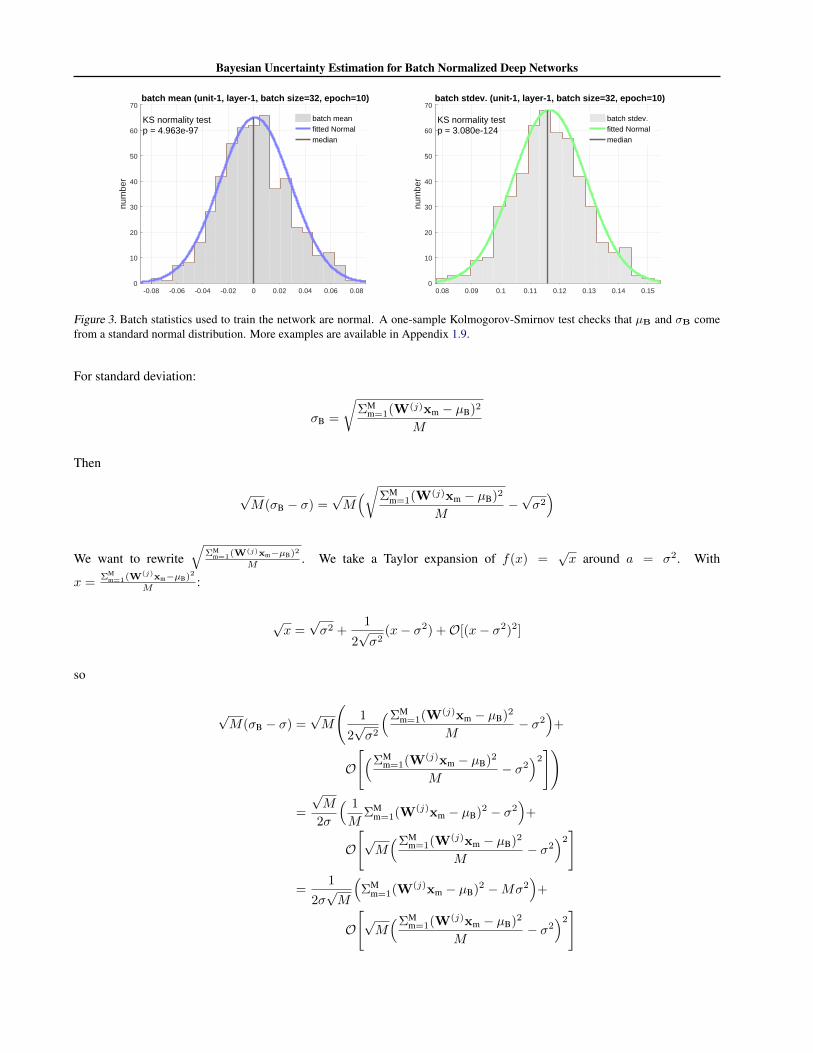
1.3. Distribution of µuB, σuBHere we approximate the distribution of mean and standard deviation of a mini-batch, separately to two Gaussians – Thishas also been empirically verified, see Figure 3 for 2 sample plots and the appendix section 1.9 for more. For the mean weget:
µB =ΣM
m=1W(j)xm
Mwhere xm are the examples in the sampled batch. We will assume these are sampled i.i.d.14. Samples of the randomvariable W(j)xm are then i.i.d.. Then by central limit theorem (CLT) the following holds for sufficiently large M (often≥ 30):
µB ∼ N (µ,σ2
M)
14Although in practice with deep learning, mini-batches are sampled without replacement, stochastic gradient descent samples withreplacement in its standard form.
Bayesian Uncertainty Estimation for Batch Normalized Deep Networks
-0.08 -0.06 -0.04 -0.02 0 0.02 0.04 0.06 0.080
10
20
30
40
50
60
70
num
ber
batch mean (unit-1, layer-1, batch size=32, epoch=10)
KS normality testp = 4.963e-97
batch meanfitted Normalmedian
0.08 0.09 0.1 0.11 0.12 0.13 0.14 0.150
10
20
30
40
50
60
70
num
ber
batch stdev. (unit-1, layer-1, batch size=32, epoch=10)
KS normality testp = 3.080e-124
batch stdev.fitted Normalmedian
Figure 3. Batch statistics used to train the network are normal. A one-sample Kolmogorov-Smirnov test checks that µB and σB comefrom a standard normal distribution. More examples are available in Appendix 1.9.
For standard deviation:
σB =
√ΣM
m=1(W(j)xm − µB)2
M
Then
√M(σB − σ) =
√M(√ΣM
m=1(W(j)xm − µB)2
M−√σ2)
We want to rewrite√
ΣMm=1(W(j)xm−µB)2
M . We take a Taylor expansion of f(x) =√x around a = σ2. With
x =ΣM
m=1(W(j)xm−µB)2
M :
√x =√σ2 +
1
2√σ2
(x− σ2) +O[(x− σ2)2]
so
√M(σB − σ) =
√M
(1
2√σ2
(ΣMm=1(W(j)xm − µB)2
M− σ2
)+
O
[(ΣMm=1(W(j)xm − µB)2
M− σ2
)2])
=
√M
2σ
( 1
MΣM
m=1(W(j)xm − µB)2 − σ2)
+
O
[√M(ΣM
m=1(W(j)xm − µB)2
M− σ2
)2]
=1
2σ√M
(ΣM
m=1(W(j)xm − µB)2 −Mσ2)
+
O
[√M(ΣM
m=1(W(j)xm − µB)2
M− σ2
)2]
Bayesian Uncertainty Estimation for Batch Normalized Deep Networks
consider ΣMm=1(W(j)xm − µB)2. We know that E[W(j)xm] = µ and write
ΣMm=1(W(j)xm − µB)2
=ΣMm=1((W(j)xm − µ)− (µB − µ))2
=ΣMm=1((W(j)xm − µ)2 + (µB − µ)2 − 2(W(j)xm − µ)(µB − µ))
=ΣMm=1(W(j)xm − µ)2 +M(µB − µ)2 − 2(µB − µ)ΣM
m=1(W(j)xm − µ)
=ΣMm=1(W(j)xm − µ)2 −M(µB − µ)2
=ΣMm=1((W(j)xm − µ)2 − (µB − µ)2)
then√M(σB − σ) =
1
2σ√M
(ΣM
m=1((W(j)xm − µ)2 − (µB − µ)2)−Mσ2)
+
O
[√M(ΣM
m=1(W(j)xm − µB)2
M− σ2
)2]
=1
2σ√M
(ΣM
m=1(W(j)xm − µ)2 − ΣMm=1(µB − µ)2 −Mσ2
)+
O
[√M(ΣM
m=1(W(j)xm − µB)2
M− σ2
)2]
=1
2σ√M
(ΣM
m=1((W(j)xm − µ)2 − σ2)− ΣMm=1(µB − µ)2
)+
O
[√M(ΣM
m=1(W(j)xm − µB)2
M− σ2
)2]
=1
2σ√M
ΣMm=1((W(j)xm − µ)2 − σ2)
− 1
2σ√M
ΣMm=1(µB − µ)2
+O
[√M(ΣM
m=1(W(j)xm − µB)2
M− σ2
)2]
=1
2σ√M
ΣMm=1((W(j)xm − µ)2 − σ2)︸ ︷︷ ︸
term A
−√M
2σ(µB − µ)2︸ ︷︷ ︸term B
+O
[√M(ΣM
m=1(W(j)xm − µB)2
M− σ2
)2]
︸ ︷︷ ︸term C
We go through each term in turn
Term AWe have
Term A =1
2σ√M
ΣMm=1((W(j)xm − µ)2 − σ2)
where ΣMm=1(W(j)xm − µ)2 is the sum of M RVs (W(j)xm − µ)2. Note that since E[W(j)xm] = µ it holds that
E[(W(j)xm − µ)2] = σ2. Since (W(j)xm − µ)2 is sampled approximately iid (by assumptions above), for large enough
Bayesian Uncertainty Estimation for Batch Normalized Deep Networks
M by CLT it holds approximately that
ΣMm=1(W(j)xm − µ)2 ∼ N (Mσ2,MVar((W(j)xm − µ)2))
where
Var((W(j)xm − µ)2) = E[(W(j)xm − µ)2∗2]− E[(W(j)xm − µ)2]2
= E[(W(j)xm − µ)4]− σ4
Then
ΣMm=1((W(j)xm − µ)2 − σ2) ∼ N (0,M ∗ E[(W(j)xm − µ)4]−Mσ4)
so
Term A ∼ N (0,E[(W(j)xm − µ)4]− σ4
4σ2)
Term BWe have
Term B =
√M
2σ(µB − µ)2 =
1
2σ
√M(µB − µ)(µB − µ)
Consider (µB − µ). As µBp−→ µ when M →∞ we have µB − µ
p−→ 0. We also have
√M(µB − µ) =
ΣMm=1W
(j)xm√M
−√Mµ
which by CLT is approximately Gaussian for large M . We can then make use of the Cramer-Slutzky Theorem, whichstates that if (Xn)n≥1 and (Yn)n≥1 are two sequences such that Xn
d−→ X and Ynp−→ a as n → ∞ where a is a constant,
then as n→∞, it holds that Xn ∗ Ynd−→ X ∗ a. Thus, Term B is approximately 0 for large M.
Term CWe have
Term C = O
[√M(ΣM
m=1(W(j)xm − µB)2
M− σ2
)2]
Since E[(W(j)xm − µ)2] = σ2 we can make the same use of Cramer-Slutzky as for Term B, such that Term C is approxi-mately 0 for large M.
Finalizing the distributionWe have approximately
√M(σB − σ) ∼ N (0,
E[(W(j)xm − µ)4]− σ4
4σ2)
so
σB ∼ N (σ,E[(W(j)xm − µ)4]− σ4
4σ2M)
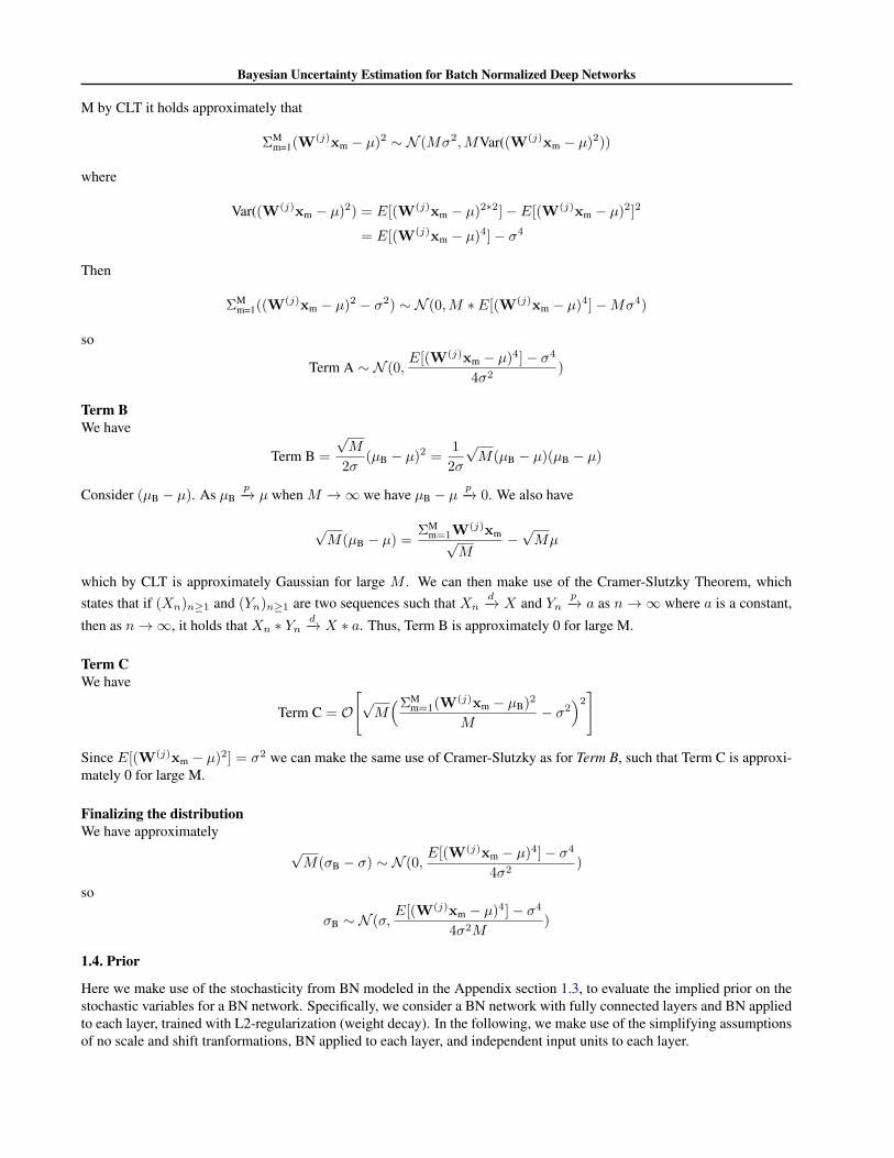
1.4. Prior
Here we make use of the stochasticity from BN modeled in the Appendix section 1.3, to evaluate the implied prior on thestochastic variables for a BN network. Specifically, we consider a BN network with fully connected layers and BN appliedto each layer, trained with L2-regularization (weight decay). In the following, we make use of the simplifying assumptionsof no scale and shift tranformations, BN applied to each layer, and independent input units to each layer.
Bayesian Uncertainty Estimation for Batch Normalized Deep Networks
Equivalence between the objectives of Eq. (1) and (2) requires:
∂
∂θkKL(qθ(ω)||p(ω)) = Nτ
∂
∂θkΩ(θ)
= Nτ∂
∂θk
L∑l=1
λl||Wl||2(5)
where θk ∈ θ, and θ is the set of weights in the network. To proceed with the LHS of Eq. (5) we first need to find theapproximate posterior qθ(ω) that batch normalization induces. As shown in Appendix 1.3, with some weak assumptionsand approximations the Central Limit Theorem (CLT) yields Gaussian distributions of the stochastic variables µuB, σ
uB, for
large enough M . For any BN unit u:
µuB ∝∼ N (µu,(σu)2
M),
σuB ∝∼ N (σu,E[(W(u)x− µu)4]− (σu)4
4(σu)2M)
(6)
where µu and σu are population-level moments (i.e. moments over D).
We assume that qθ(ω) and p(ω) factorize over all stochastic variables.15 We use i as an index of the set of stochasticvariables. As shown in Eq. (3) in Appendix 1.2, the factorized distributions yield:
KL(qθ(ω)||p(ω)) =∑i
KL(qθ(ωi)||p(ωi))
Note that each BN unit produces two KL(qθ(ωi)||p(ωi)) terms: one for ωi = µuB and one for ωi = σuB. We consider theseterms for one particular BN unit u, and drop the index i for brevity. We use a Gaussian prior p(ωi) = N (µp, σ
2p) and, for
consistency, use the notation qθ(ωi) = N (µq, σ2q ). As shown in Eq. (4) in Appendix 1.2:
KL(qθ(ωi)||p(ωi)) = lnσpσq
+σ2q + (µq − µp)2
2σ2p
− 1
2
Since θk changes during training, a prior cannot depend on θk so ∂∂θk
(µp) = ∂∂θk
(σp) = 0. Letting (·)′ denote ∂∂θk
(·):
∂
∂θkKL(qθ(ωi)||p(ωi)) =
σqσ′q + µqµ
′q − µpµ′q
σ2p
−σ′qσq
(7)
We need not consider θk past a previous layer’s BN, since a normalization step is performed before scale and shift. In thegeneral case with a given Gaussian p(ω), Eq. 7 evaluated on all BN units’ means and standard deviations w.r.t. all θk up toa previous layer’s BN, would yield an expression for a custom Nτ ∂
∂θkΩ(θ) that could be used for an exact VI treatment of
BN.
In our reconciliation of weight decay however, given our assumptions of no scale and shift and BN applied to each layer,we need only consider the weights in the same layer as the BN unit. This means that the stochastic variables in layer l areonly affected by weights in θk ∈W l (i.e. not the scale and shift variables operating on the input to the layer). We denotea weight connecting the k:th input unit to the u:th BN unit by W(u,k). For such weights, we need to derive µ′q and σ′q , fortwo cases: ωi = µuB and ωi = σuB. We denote the priors of the mean and std. dev for µuB by µµ,q and σµ,q , and for σuB byµσ,q and σσ,q . Using the distributions modeled in Eq. 6:
15The empirical distributions have been numerically checked to be linearly independent and the joint distribution is close to a bi-variateGaussian.
Bayesian Uncertainty Estimation for Batch Normalized Deep Networks
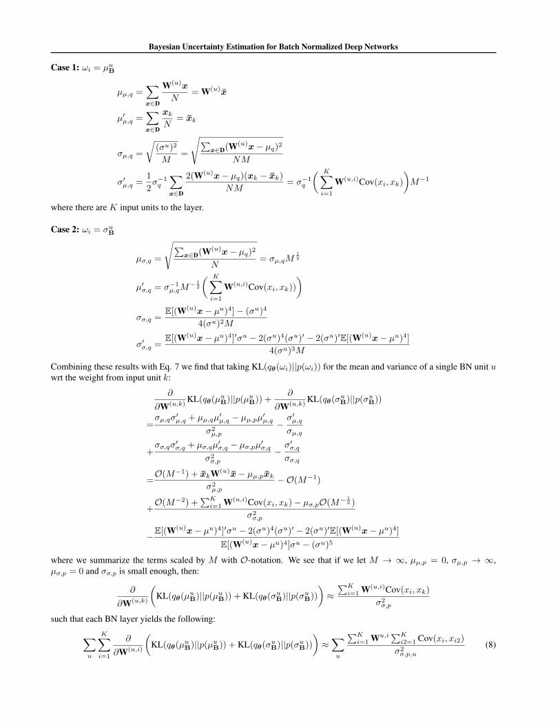
Case 1: ωi = µuB
µµ,q =∑x∈D
W(u)x
N= W(u)x
µ′µ,q =∑x∈D
xkN
= xk
σµ,q =
√(σu)2
M=
√∑x∈D(W(u)x− µq)2
NM
σ′µ,q =1
2σ−1q
∑x∈D
2(W(u)x− µq)(xk − xk)
NM= σ−1
q
( K∑i=1
W(u,i)Cov(xi, xk)
)M−1
where there are K input units to the layer.
Case 2: ωi = σuB
µσ,q =
√∑x∈D(W(u)x− µq)2
N= σµ,qM
12
µ′σ,q = σ−1µ,qM
− 12
( K∑i=1
W(u,i)Cov(xi, xk))
)
σσ,q =E[(W(u)x− µu)4]− (σu)4
4(σu)2M
σ′σ,q =E[(W(u)x− µu)4]′σu − 2(σu)4(σu)′ − 2(σu)′E[(W(u)x− µu)4]
4(σu)3M
Combining these results with Eq. 7 we find that taking KL(qθ(ωi)||p(ωi)) for the mean and variance of a single BN unit uwrt the weight from input unit k:
∂
∂W(u,k)KL(qθ(µuB)||p(µuB)) +
∂
∂W(u,k)KL(qθ(σuB)||p(σuB))
=σµ,qσ
′µ,q + µµ,qµ
′µ,q − µµ,pµ′µ,q
σ2µ,p
−σ′µ,qσµ,q
+σσ,qσ
′σ,q + µσ,qµ
′σ,q − µσ,pµ′σ,q
σ2σ,p
−σ′σ,qσσ,q
=O(M−1) + xkW(u)x− µµ,pxk
σ2µ,p
−O(M−1)
+O(M−2) +
∑Ki=1 W(u,i)Cov(xi, xk)− µσ,pO(M−
12 )
σ2σ,p
−E[(W(u)x− µu)4]′σu − 2(σu)4(σu)′ − 2(σu)′E[(W(u)x− µu)4]
E[(W(u)x− µu)4]σu − (σu)5
where we summarize the terms scaled by M with O-notation. We see that if we let M → ∞, µµ,p = 0, σµ,p → ∞,µσ,p = 0 and σσ,p is small enough, then:
∂
∂W(u,k)
(KL(qθ(µuB)||p(µuB)) + KL(qθ(σuB)||p(σuB))
)≈∑Ki=1 W(u,i)Cov(xi, xk)
σ2σ,p
such that each BN layer yields the following:∑u
K∑i=1
∂
∂W(u,i)
(KL(qθ(µuB)||p(µuB)) + KL(qθ(σuB)||p(σuB))
)≈∑u
∑Ki=1 Wu,i∑K
i2=1 Cov(xi, xi2)
σ2σ,p,u
(8)

Bayesian Uncertainty Estimation for Batch Normalized Deep Networks
where we denote the prior for the std. dev. of the std. dev. of BN unit u by σσ,p,u. Given our assumptions of no scale andshift from the previous layer, and independent input features in every layer, Eq. 8 reduces to:
∑u
K∑i=1
Wu,i
σ2σ,p
if the same prior is chosen for each BN unit in the layer. We therefore find that Eq. 5 is reconciled by p(µuB)→ N (0,∞)and p(σuB)→ N (0, 1
2Nτλl), if 1
2Nτλlis small enough, which is the case if N is large.
1.5. predictive distribution properties
This section provides derivations of properties of the predictive distribution p∗(y|x,D) in section 3.4, following (Gal,2016). We first find the first two modes of the approximate predictive distribution (with the second mode applicable toregression), then show how to estimate the predictive log likelihood, a measure of uncertainty quality used in the evaluation.
Predictive mean Assuming Gaussian iid noise defined by model precision τ , i.e. fω(x,y) = p(y|fω(x)) =N (y; fω(x), τ−1I):
Ep∗ [y] =
∫yp∗(y|x,D)dy
=
∫y
y(∫
ω
fω(x,y)qθ(ω)dω)
dy
=
∫y
y(∫
ω
N (y; fω(x), τ−1I)qθ(ω)dω)
dy
=
∫ω
(∫y
yN (y; fω(x), τ−1I)dy)qθ(ω)dω
=
∫ω
fω(x)qθ(ω)dω
≈ 1
T
T∑i=1
fωi(x)
where we take the MC Integral with T samples of ω for the approximation in the final step.
Predictive variance For regression, our goal is to estimate:
Covp∗ [y] = Ep∗ [yᵀy]− Ep∗ [y]ᵀEp∗ [y]
We find that:
Ep∗ [yᵀy] =
∫y
yᵀyp∗(y|x,D)dy
=
∫y
yᵀy(∫
ω
fω(x,y)qθ(ω)dω)
dy
=
∫ω
(∫y
yᵀyfω(x,y)dy)qθ(ω)dω
=
∫ω
(Covfω(x,y)(y) + Efω(x,y)[y]ᵀEfω(x,y)[y]
)qθ(ω)dω
=
∫ω
(τ−1I + fω(x)ᵀfω(x)
)qθ(ω)dω
= τ−1I + Eqθ(ω)[fω(x)ᵀfω(x)]
≈ τ−1I +1
T
T∑i=1
fωi(x)ᵀfωi
(x)
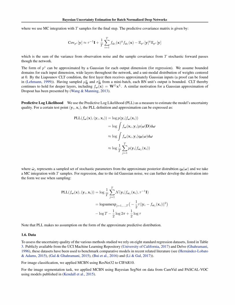
Bayesian Uncertainty Estimation for Batch Normalized Deep Networks
where we use MC integration with T samples for the final step. The predictive covariance matrix is given by:
Covp∗ [y] ≈ τ−1I +1
T
T∑i=1
fωi(x)ᵀfωi
(x)− Ep∗ [y]ᵀEp∗ [y]
which is the sum of the variance from observation noise and the sample covariance from T stochastic forward passesthough the network.
The form of p∗ can be approximated by a Gaussian for each output dimension (for regression). We assume boundeddomains for each input dimension, wide layers throughout the network, and a uni-modal distribution of weights centeredat 0. By the Liapounov CLT condition, the first layer then receives approximately Gaussian inputs (a proof can be foundin (Lehmann, 1999)). Having sampled µuB and σuB from a mini-batch, each BN unit’s output is bounded. CLT therebycontinues to hold for deeper layers, including fω(x) = WLxL. A similar motivation for a Gaussian approximation ofDropout has been presented by (Wang & Manning, 2013).
Predictive Log Likelihood We use the Predictive Log Likelihood (PLL) as a measure to estimate the model’s uncertaintyquality. For a certain test point (yi,xi), the PLL definition and approximation can be expressed as:
PLL(fω(x), (yi,xi)) = log p(yi|fω(xi))
= log
∫fω(xi,yi)p(ω|D)dω
≈ log
∫fω(xi,yi)qθ(ω)dω
≈ log1
T
T∑j=1
p(yi|fωj(xi))
where ωj represents a sampled set of stochastic parameters from the approximate posterior distrubtion qθ(ω) and we takea MC integration with T samples. For regression, due to the iid Gaussian noise, we can further develop the derivation intothe form we use when sampling:
PLL(fω(x), (yi,xi)) = log1
T
T∑j=1
N (yi|fωj(xi), τ
−1I)
= logsumexpj=1,...,T
(− 1
2τ ||yi − fωj
(xi)||2)
− log T − 1
2log 2π +
1
2log τ
Note that PLL makes no assumption on the form of the approximate predictive distribution.
1.6. Data
To assess the uncertainty quality of the various methods studied we rely on eight standard regression datasets, listed in Table3. Publicly available from the UCI Machine Learning Repository (University of California, 2017) and Delve (Ghahramani,1996), these datasets have been used to benchmark comparative models in recent related literature (see (Hernandez-Lobato& Adams, 2015), (Gal & Ghahramani, 2015), (Bui et al., 2016) and (Li & Gal, 2017)).
For image classification, we applied MCBN using ResNet32 to CIFAR10.
For the image segmentation task, we applied MCBN using Bayesian SegNet on data from CamVid and PASCAL-VOCusing models published in (Kendall et al., 2015).
Bayesian Uncertainty Estimation for Batch Normalized Deep Networks
Table 3. Regression dataset summary. Properties of the eight regression datasets used to evaluate MCBN. N is the dataset size and Qis the n.o. input features. Only one target feature was used – we used heating load for the Energy Efficiency dataset, which containsmultiple target features.
Dataset name N Q
Boston Housing 506 13Concrete Compressive Strength 1,030 8Energy Efficiency 768 8Kinematics 8nm 8,192 8Power Plant 9,568 4Protein Tertiary Structure 45,730 9Wine Quality (Red) 1,599 11Yacht Hydrodynamics 308 6
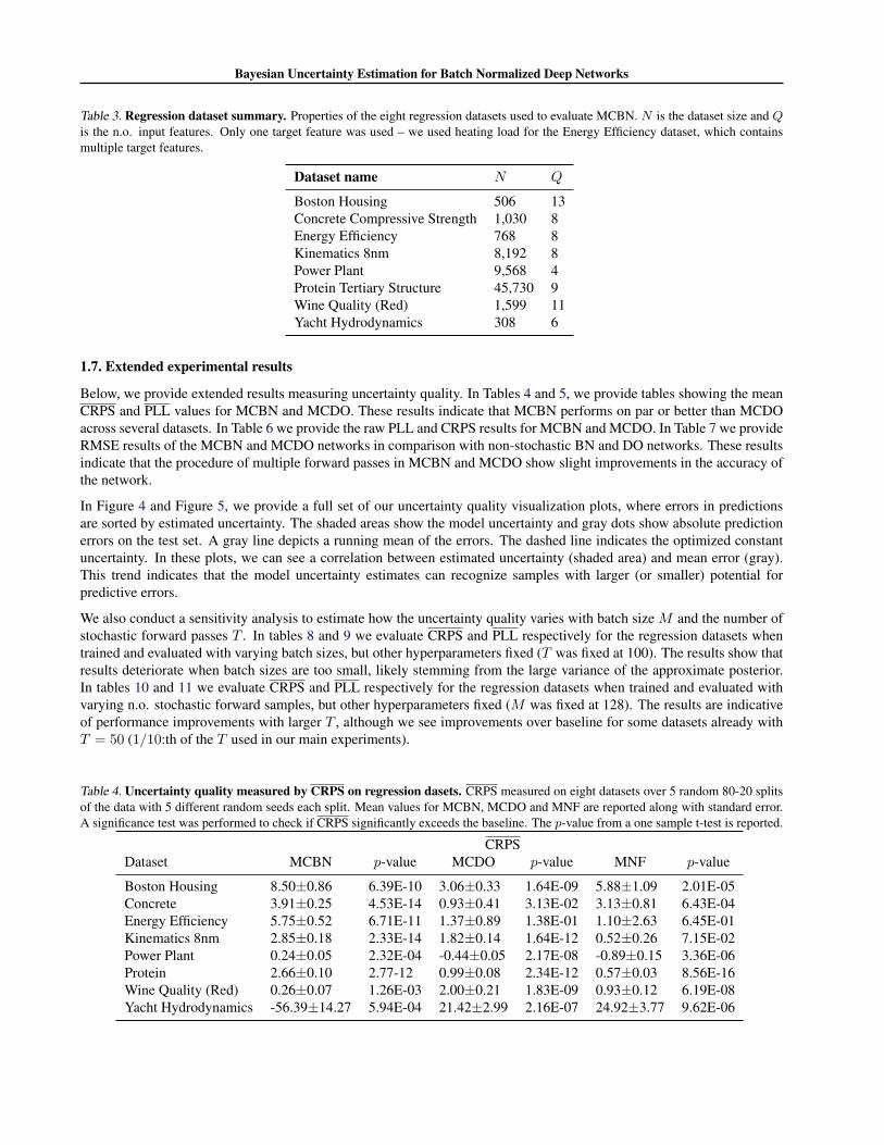
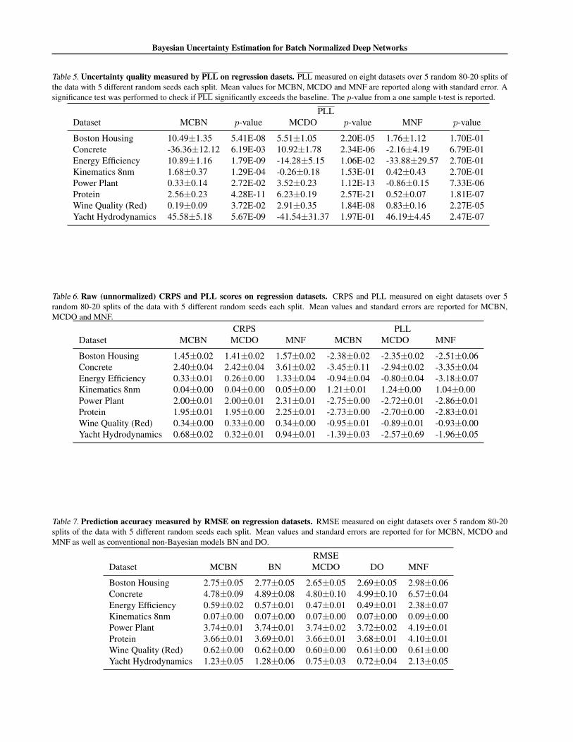
1.7. Extended experimental results
Below, we provide extended results measuring uncertainty quality. In Tables 4 and 5, we provide tables showing the meanCRPS and PLL values for MCBN and MCDO. These results indicate that MCBN performs on par or better than MCDOacross several datasets. In Table 6 we provide the raw PLL and CRPS results for MCBN and MCDO. In Table 7 we provideRMSE results of the MCBN and MCDO networks in comparison with non-stochastic BN and DO networks. These resultsindicate that the procedure of multiple forward passes in MCBN and MCDO show slight improvements in the accuracy ofthe network.
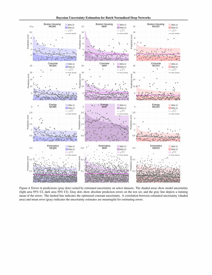
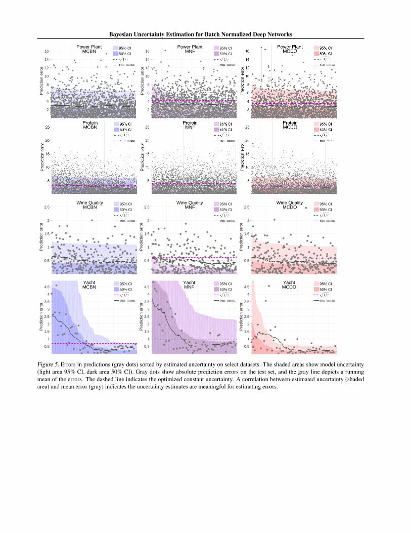
In Figure 4 and Figure 5, we provide a full set of our uncertainty quality visualization plots, where errors in predictionsare sorted by estimated uncertainty. The shaded areas show the model uncertainty and gray dots show absolute predictionerrors on the test set. A gray line depicts a running mean of the errors. The dashed line indicates the optimized constantuncertainty. In these plots, we can see a correlation between estimated uncertainty (shaded area) and mean error (gray).This trend indicates that the model uncertainty estimates can recognize samples with larger (or smaller) potential forpredictive errors.
We also conduct a sensitivity analysis to estimate how the uncertainty quality varies with batch size M and the number ofstochastic forward passes T . In tables 8 and 9 we evaluate CRPS and PLL respectively for the regression datasets whentrained and evaluated with varying batch sizes, but other hyperparameters fixed (T was fixed at 100). The results show thatresults deteriorate when batch sizes are too small, likely stemming from the large variance of the approximate posterior.In tables 10 and 11 we evaluate CRPS and PLL respectively for the regression datasets when trained and evaluated withvarying n.o. stochastic forward samples, but other hyperparameters fixed (M was fixed at 128). The results are indicativeof performance improvements with larger T , although we see improvements over baseline for some datasets already withT = 50 (1/10:th of the T used in our main experiments).
Table 4. Uncertainty quality measured by CRPS on regression dasets. CRPS measured on eight datasets over 5 random 80-20 splitsof the data with 5 different random seeds each split. Mean values for MCBN, MCDO and MNF are reported along with standard error.A significance test was performed to check if CRPS significantly exceeds the baseline. The p-value from a one sample t-test is reported.
CRPSDataset MCBN p-value MCDO p-value MNF p-value
Boston Housing 8.50±0.86 6.39E-10 3.06±0.33 1.64E-09 5.88±1.09 2.01E-05Concrete 3.91±0.25 4.53E-14 0.93±0.41 3.13E-02 3.13±0.81 6.43E-04Energy Efficiency 5.75±0.52 6.71E-11 1.37±0.89 1.38E-01 1.10±2.63 6.45E-01Kinematics 8nm 2.85±0.18 2.33E-14 1.82±0.14 1.64E-12 0.52±0.26 7.15E-02Power Plant 0.24±0.05 2.32E-04 -0.44±0.05 2.17E-08 -0.89±0.15 3.36E-06Protein 2.66±0.10 2.77-12 0.99±0.08 2.34E-12 0.57±0.03 8.56E-16Wine Quality (Red) 0.26±0.07 1.26E-03 2.00±0.21 1.83E-09 0.93±0.12 6.19E-08Yacht Hydrodynamics -56.39±14.27 5.94E-04 21.42±2.99 2.16E-07 24.92±3.77 9.62E-06
Bayesian Uncertainty Estimation for Batch Normalized Deep Networks
Table 5. Uncertainty quality measured by PLL on regression dasets. PLL measured on eight datasets over 5 random 80-20 splits ofthe data with 5 different random seeds each split. Mean values for MCBN, MCDO and MNF are reported along with standard error. Asignificance test was performed to check if PLL significantly exceeds the baseline. The p-value from a one sample t-test is reported.
PLLDataset MCBN p-value MCDO p-value MNF p-value
Boston Housing 10.49±1.35 5.41E-08 5.51±1.05 2.20E-05 1.76±1.12 1.70E-01Concrete -36.36±12.12 6.19E-03 10.92±1.78 2.34E-06 -2.16±4.19 6.79E-01Energy Efficiency 10.89±1.16 1.79E-09 -14.28±5.15 1.06E-02 -33.88±29.57 2.70E-01Kinematics 8nm 1.68±0.37 1.29E-04 -0.26±0.18 1.53E-01 0.42±0.43 2.70E-01Power Plant 0.33±0.14 2.72E-02 3.52±0.23 1.12E-13 -0.86±0.15 7.33E-06Protein 2.56±0.23 4.28E-11 6.23±0.19 2.57E-21 0.52±0.07 1.81E-07Wine Quality (Red) 0.19±0.09 3.72E-02 2.91±0.35 1.84E-08 0.83±0.16 2.27E-05Yacht Hydrodynamics 45.58±5.18 5.67E-09 -41.54±31.37 1.97E-01 46.19±4.45 2.47E-07
Table 6. Raw (unnormalized) CRPS and PLL scores on regression datasets. CRPS and PLL measured on eight datasets over 5random 80-20 splits of the data with 5 different random seeds each split. Mean values and standard errors are reported for MCBN,MCDO and MNF.
CRPS PLLDataset MCBN MCDO MNF MCBN MCDO MNF
Boston Housing 1.45±0.02 1.41±0.02 1.57±0.02 -2.38±0.02 -2.35±0.02 -2.51±0.06Concrete 2.40±0.04 2.42±0.04 3.61±0.02 -3.45±0.11 -2.94±0.02 -3.35±0.04Energy Efficiency 0.33±0.01 0.26±0.00 1.33±0.04 -0.94±0.04 -0.80±0.04 -3.18±0.07Kinematics 8nm 0.04±0.00 0.04±0.00 0.05±0.00 1.21±0.01 1.24±0.00 1.04±0.00Power Plant 2.00±0.01 2.00±0.01 2.31±0.01 -2.75±0.00 -2.72±0.01 -2.86±0.01Protein 1.95±0.01 1.95±0.00 2.25±0.01 -2.73±0.00 -2.70±0.00 -2.83±0.01Wine Quality (Red) 0.34±0.00 0.33±0.00 0.34±0.00 -0.95±0.01 -0.89±0.01 -0.93±0.00Yacht Hydrodynamics 0.68±0.02 0.32±0.01 0.94±0.01 -1.39±0.03 -2.57±0.69 -1.96±0.05
Table 7. Prediction accuracy measured by RMSE on regression datasets. RMSE measured on eight datasets over 5 random 80-20splits of the data with 5 different random seeds each split. Mean values and standard errors are reported for for MCBN, MCDO andMNF as well as conventional non-Bayesian models BN and DO.
RMSEDataset MCBN BN MCDO DO MNF
Boston Housing 2.75±0.05 2.77±0.05 2.65±0.05 2.69±0.05 2.98±0.06Concrete 4.78±0.09 4.89±0.08 4.80±0.10 4.99±0.10 6.57±0.04Energy Efficiency 0.59±0.02 0.57±0.01 0.47±0.01 0.49±0.01 2.38±0.07Kinematics 8nm 0.07±0.00 0.07±0.00 0.07±0.00 0.07±0.00 0.09±0.00Power Plant 3.74±0.01 3.74±0.01 3.74±0.02 3.72±0.02 4.19±0.01Protein 3.66±0.01 3.69±0.01 3.66±0.01 3.68±0.01 4.10±0.01Wine Quality (Red) 0.62±0.00 0.62±0.00 0.60±0.00 0.61±0.00 0.61±0.00Yacht Hydrodynamics 1.23±0.05 1.28±0.06 0.75±0.03 0.72±0.04 2.13±0.05
Bayesian Uncertainty Estimation for Batch Normalized Deep Networks
2
4
6
8
10
12P
redi
ctio
n er
ror
Boston HousingMCBN
95% CI
50% CI
2
4
6
8
10
12
Pre
dict
ion
erro
r
Boston HousingMNF
95% CI
50% CI
2
4
6
8
10
12
Pre
dict
ion
erro
r
Boston HousingMCDO
95% CI
50% CI
5
10
15
20
25
Pre
dict
ion
erro
r
ConcreteMCBN
95% CI
50% CI
5
10
15
20
25
Pre
dict
ion
erro
r
ConcreteMNF
95% CI
50% CI
5
10
15
20
25
Pre
dict
ion
erro
r
ConcreteMCDO
95% CI
50% CI
0.5
1
1.5
2
2.5
3
Pre
dict
ion
erro
r
EnergyMCBN
95% CI
50% CI
0.5
1
1.5
2
2.5
3
Pre
dict
ion
erro
r
EnergyMNF
95% CI
50% CI
0.5
1
1.5
2
2.5
3
Pre
dict
ion
erro
r
EnergyMCDO
95% CI
50% CI
0.1
0.2
0.3
Pre
dict
ion
erro
r
KinematicsMCBN
95% CI
50% CI
0.1
0.2
0.3
Pre
dict
ion
erro
r
KinematicsMNF
95% CI
50% CI
0.1
0.2
0.3
Pre
dict
ion
erro
r
KinematicsMCDO
95% CI
50% CI
Figure 4. Errors in predictions (gray dots) sorted by estimated uncertainty on select datasets. The shaded areas show model uncertainty(light area 95% CI, dark area 50% CI). Gray dots show absolute prediction errors on the test set, and the gray line depicts a runningmean of the errors. The dashed line indicates the optimized constant uncertainty. A correlation between estimated uncertainty (shadedarea) and mean error (gray) indicates the uncertainty estimates are meaningful for estimating errors.
Bayesian Uncertainty Estimation for Batch Normalized Deep Networks
2
4
6
8
10
12
14
16
Pre
dict
ion
erro
rPower Plant
MCBN95% CI
50% CI
2
4
6
8
10
12
14
16
Pre
dict
ion
erro
r
Power PlantMNF
95% CI
50% CI
0.5
1
1.5
2
2.5
Pre
dict
ion
erro
r
Wine QualityMCBN
95% CI
50% CI
0.5
1
1.5
2
2.5
Pre
dict
ion
erro
r
Wine QualityMNF
95% CI
50% CI
0.5
1
1.5
2
2.5
Pre
dict
ion
erro
r
Wine QualityMCDO
95% CI
50% CI
0.5
1
1.5
2
2.5
3
3.5
4
4.5
Pre
dict
ion
erro
r
YachtMCBN
95% CI
50% CI
0.5
1
1.5
2
2.5
3
3.5
4
4.5
Pre
dict
ion
erro
r
YachtMNF
95% CI
50% CI
0.5
1
1.5
2
2.5
3
3.5
4
4.5
Pre
dict
ion
erro
r
YachtMCDO
95% CI
50% CI
Figure 5. Errors in predictions (gray dots) sorted by estimated uncertainty on select datasets. The shaded areas show model uncertainty(light area 95% CI, dark area 50% CI). Gray dots show absolute prediction errors on the test set, and the gray line depicts a runningmean of the errors. The dashed line indicates the optimized constant uncertainty. A correlation between estimated uncertainty (shadedarea) and mean error (gray) indicates the uncertainty estimates are meaningful for estimating errors.
Bayesian Uncertainty Estimation for Batch Normalized Deep Networks
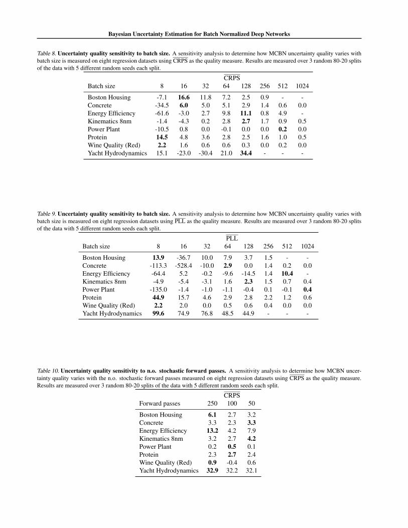
Table 8. Uncertainty quality sensitivity to batch size. A sensitivity analysis to determine how MCBN uncertainty quality varies withbatch size is measured on eight regression datasets using CRPS as the quality measure. Results are measured over 3 random 80-20 splitsof the data with 5 different random seeds each split.
CRPSBatch size 8 16 32 64 128 256 512 1024
Boston Housing -7.1 16.6 11.8 7.2 2.5 0.9 - -Concrete -34.5 6.0 5.0 5.1 2.9 1.4 0.6 0.0Energy Efficiency -61.6 -3.0 2.7 9.8 11.1 0.8 4.9 -Kinematics 8nm -1.4 -4.3 0.2 2.8 2.7 1.7 0.9 0.5Power Plant -10.5 0.8 0.0 -0.1 0.0 0.0 0.2 0.0Protein 14.5 4.8 3.6 2.8 2.5 1.6 1.0 0.5Wine Quality (Red) 2.2 1.6 0.6 0.6 0.3 0.0 0.2 0.0Yacht Hydrodynamics 15.1 -23.0 -30.4 21.0 34.4 - - -
Table 9. Uncertainty quality sensitivity to batch size. A sensitivity analysis to determine how MCBN uncertainty quality varies withbatch size is measured on eight regression datasets using PLL as the quality measure. Results are measured over 3 random 80-20 splitsof the data with 5 different random seeds each split.
PLLBatch size 8 16 32 64 128 256 512 1024
Boston Housing 13.9 -36.7 10.0 7.9 3.7 1.5 - -Concrete -113.3 -528.4 -10.0 2.9 0.0 1.4 0.2 0.0Energy Efficiency -64.4 5.2 -0.2 -9.6 -14.5 1.4 10.4 -Kinematics 8nm -4.9 -5.4 -3.1 1.6 2.3 1.5 0.7 0.4Power Plant -135.0 -1.4 -1.0 -1.1 -0.4 0.1 -0.1 0.4Protein 44.9 15.7 4.6 2.9 2.8 2.2 1.2 0.6Wine Quality (Red) 2.2 2.0 0.0 0.5 0.6 0.4 0.0 0.0Yacht Hydrodynamics 99.6 74.9 76.8 48.5 44.9 - - -
Table 10. Uncertainty quality sensitivity to n.o. stochastic forward passes. A sensitivity analysis to determine how MCBN uncer-tainty quality varies with the n.o. stochastic forward passes measured on eight regression datasets using CRPS as the quality measure.Results are measured over 3 random 80-20 splits of the data with 5 different random seeds each split.
CRPSForward passes 250 100 50
Boston Housing 6.1 2.7 3.2Concrete 3.3 2.3 3.3Energy Efficiency 13.2 4.2 7.9Kinematics 8nm 3.2 2.7 4.2Power Plant 0.2 0.5 0.1Protein 2.3 2.7 2.4Wine Quality (Red) 0.9 -0.4 0.6Yacht Hydrodynamics 32.9 32.2 32.1
Bayesian Uncertainty Estimation for Batch Normalized Deep Networks
Table 11. Uncertainty quality sensitivity to n.o. stochastic forward passes. A sensitivity analysis to determine how MCBN uncer-tainty quality varies with the n.o. stochastic forward passes measured on eight regression datasets using PLL as the quality measure.Results are measured over 3 random 80-20 splits of the data with 5 different random seeds each split.
PLLForward passes 250 100 50
Boston Housing 7.8 1.9 2.6Concrete 3.8 7.1 0.1Energy Efficiency 15.7 -30.5 -47.3Kinematics 8nm 2.5 2.2 3.4Power Plant -0.9 0.7 -0.9Protein 1.8 2.0 2.4Wine Quality (Red) 1.7 -0.9 1.1Yacht Hydrodynamics 38.0 35.9 35.5
1.8. Uncertainty in image segmentation
We applied MCBN to an image segmentation task using Bayesian SegNet with the main CamVid and PASCAL-VOCmodels in (Kendall et al., 2015). Here, we provide more image from Pascal VOC dataset in Figure 6.
1.9. Batch normalization statistics
In Figure 7 and Figure 8, we provide statistics on the batch normalization parameters used for training. The plots show thedistribution of BN mean and BN variance over different mini-batches of an actual training of Yacht dataset for one unit inthe first hidden layer and the second hidden layer. Data is provided for different epochs and for different batch sizes.
Bayesian Uncertainty Estimation for Batch Normalized Deep Networks
Figure 6. Uncertainty in image segmentation. Results applying MCBN to Bayesian SegNet (Kendall et al., 2015) on images fromPASCAL-VOC (right). Left: original. Middle: the Bayesian estimated segmentation. Right: estimated uncertainty using MCBN for allclasses. Mini-batches of size 36 were used for PASCAL-VOC on images of size 224x224. 20 inferences were conducted to estimate themean and variance of MCBN.

Bayesian Uncertainty Estimation for Batch Normalized Deep Networks
-0.08 -0.06 -0.04 -0.02 0 0.02 0.04 0.06 0.080
10
20
30
40
50
60
70
num
ber
batch mean (unit-1, layer-1, batch size=32, epoch=10)
KS normality testp = 4.963e-97
batch meanfitted Normalmedian
-0.02 -0.015 -0.01 -0.005 0 0.005 0.01 0.015 0.020
10
20
30
40
50
60
70
80
num
ber
batch mean (unit-1, layer-1, batch size=32, epoch=100)
KS normality testp = 2.668e-106
batch meanfitted Normalmedian
-0.06 -0.04 -0.02 0 0.02 0.04 0.060
10
20
30
40
50
60
70
80
num
ber
batch mean (unit-1, layer-1, batch size=128, epoch=10)
KS normality testp = 6.353e-101
batch meanfitted Normalmedian
-6 -4 -2 0 2 4 6 8
10-3
0
10
20
30
40
50
60
70
num
ber
batch mean (unit-1, layer-1, batch size=128, epoch=100)
KS normality testp = 9.099e-109
batch meanfitted Normalmedian
0.06 0.065 0.07 0.075 0.080
10
20
30
40
50
60
70
80
num
ber
batch mean (unit-1, layer-2, batch size=32, epoch=10)
KS normality testp = 3.107e-120
batch meanfitted Normalmedian
-9.5 -9 -8.5 -8 -7.5 -7 -6.5 -6
10-3
0
10
20
30
40
50
60
70
num
ber
batch mean (unit-1, layer-2, batch size=32, epoch=100)
KS normality testp = 5.401e-111
batch meanfitted Normalmedian
0.072 0.074 0.076 0.078 0.08 0.082 0.084 0.086 0.088 0.09 0.0920
10
20
30
40
50
60
70
num
ber
batch mean (unit-1, layer-2, batch size=128, epoch=10)
KS normality testp = 8.417e-123
batch meanfitted Normalmedian
0.021 0.0215 0.022 0.0225 0.0230
10
20
30
40
50
60
num
ber
batch mean (unit-1, layer-2, batch size=128, epoch=100)
KS normality testp = 1.393e-113
batch meanfitted Normalmedian
Figure 7. The distribution of means of mini-batches during training of one of our datasets. The distribution closely follows our analyt-ically approximated Gaussian distribution. The data is collected for one unit of each layer and is provided for different epochs and fordifferent batch sizes.
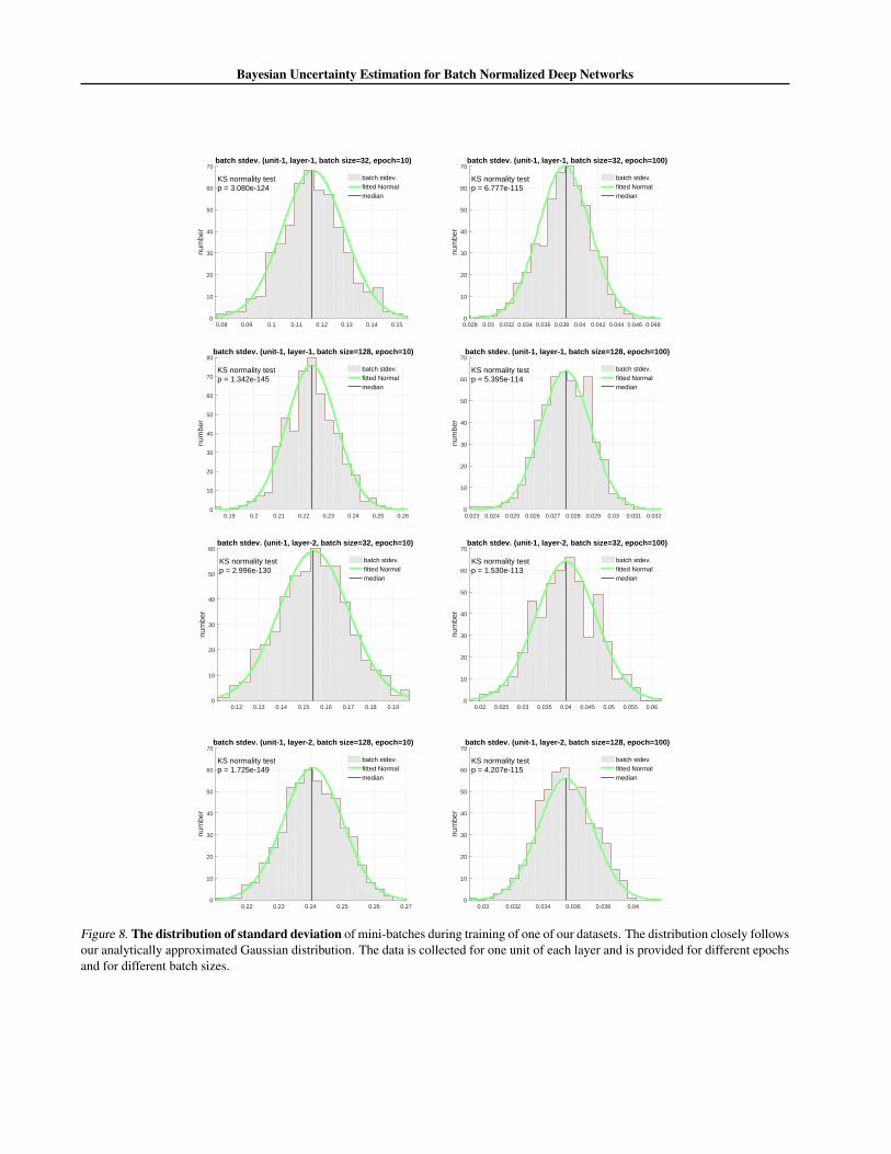
Bayesian Uncertainty Estimation for Batch Normalized Deep Networks
0.08 0.09 0.1 0.11 0.12 0.13 0.14 0.150
10
20
30
40
50
60
70
num
ber
batch stdev. (unit-1, layer-1, batch size=32, epoch=10)
KS normality testp = 3.080e-124
batch stdev.fitted Normalmedian
0.028 0.03 0.032 0.034 0.036 0.038 0.04 0.042 0.044 0.046 0.0480
10
20
30
40
50
60
70
num
ber
batch stdev. (unit-1, layer-1, batch size=32, epoch=100)
KS normality testp = 6.777e-115
batch stdev.fitted Normalmedian
0.19 0.2 0.21 0.22 0.23 0.24 0.25 0.260
10
20
30
40
50
60
70
80
num
ber
batch stdev. (unit-1, layer-1, batch size=128, epoch=10)
KS normality testp = 1.342e-145
batch stdev.fitted Normalmedian
0.023 0.024 0.025 0.026 0.027 0.028 0.029 0.03 0.031 0.0320
10
20
30
40
50
60
70
num
ber
batch stdev. (unit-1, layer-1, batch size=128, epoch=100)
KS normality testp = 5.395e-114
batch stdev.fitted Normalmedian
0.12 0.13 0.14 0.15 0.16 0.17 0.18 0.190
10
20
30
40
50
60
num
ber
batch stdev. (unit-1, layer-2, batch size=32, epoch=10)
KS normality testp = 2.996e-130
batch stdev.fitted Normalmedian
0.02 0.025 0.03 0.035 0.04 0.045 0.05 0.055 0.060
10
20
30
40
50
60
70
num
ber
batch stdev. (unit-1, layer-2, batch size=32, epoch=100)
KS normality testp = 1.530e-113
batch stdev.fitted Normalmedian
0.22 0.23 0.24 0.25 0.26 0.270
10
20
30
40
50
60
70
num
ber
batch stdev. (unit-1, layer-2, batch size=128, epoch=10)
KS normality testp = 1.725e-149
batch stdev.fitted Normalmedian
0.03 0.032 0.034 0.036 0.038 0.040
10
20
30
40
50
60
70
num
ber
batch stdev. (unit-1, layer-2, batch size=128, epoch=100)
KS normality testp = 4.207e-115
batch stdev.fitted Normalmedian
Figure 8. The distribution of standard deviation of mini-batches during training of one of our datasets. The distribution closely followsour analytically approximated Gaussian distribution. The data is collected for one unit of each layer and is provided for different epochsand for different batch sizes.

Bayesian Uncertainty Estimation for Batch Normalized Deep Networks
ReferencesBui, T. D., Hernandez-Lobato, D., Li, Y., Hernandez-Lobato, J. M., and Turner, R. E. Deep Gaussian Processes for
Regression using Approximate Expectation Propagation. In ICML, 2016.
Chen, X., Kundu, K., Zhang, Z., Ma, H., Fidler, S., and Urtasun, R. Monocular 3d object detection for autonomous driving.In Proceedings of the IEEE Conference on Computer Vision and Pattern Recognition, pp. 2147–2156, 2016.
Djuric, U., Zadeh, G., Aldape, K., and Diamandis, P. Precision histology: how deep learning is poised to revitalizehistomorphology for personalized cancer care. npj Precision Oncology, 1(1):22, 2017.
Esteva, A., Kuprel, B., Novoa, R. A., Ko, J., Swetter, S. M., Blau, H. M., and Thrun, S. Dermatologist-level classificationof skin cancer with deep neural networks. Nature, Feb 2017.
Gal, Y. Uncertainty in Deep Learning. PhD thesis, University of Cambridge, 2016.
Gal, Y. and Ghahramani, Z. Dropout as a Bayesian Approximation : Representing Model Uncertainty in Deep Learning.ICML, 48:1–10, 2015.
Ghahramani, Z. Delve Datasets. University of Toronto, 1996. URL http://www.cs.toronto.edu/˜delve/data/kin/desc.html.
Ghahramani, Z. Probabilistic machine learning and artificial intelligence. Nature, 521(7553):452–459, May 2015.
Gneiting, T. and Raftery, A. E. Strictly Proper Scoring Rules, Prediction, and Estimation. Journal of the AmericanStatistical Association, 102(477):359–378, 2007.
Goodfellow, I. J., Shlens, J., and Szegedy, C. Explaining and harnessing adversarial examples. arXiv preprintarXiv:1412.6572, 2014.
Graves, A. Practical Variational Inference for Neural Networks. NIPS, 2011.
Hernandez-Lobato, J. M. and Adams, R. Probabilistic backpropagation for scalable learning of bayesian neural networks.In International Conference on Machine Learning, pp. 1861–1869, 2015.
Hinton, G. E. and Van Camp, D. Keeping the neural networks simple by minimizing the description length of the weights.In Proceedings of the sixth annual conference on Computational learning theory, pp. 5–13. ACM, 1993.
Ioffe, S. Batch renormalization: Towards reducing minibatch dependence in batch-normalized models. CoRR,abs/1702.03275, 2017. URL http://arxiv.org/abs/1702.03275.
Ioffe, S. and Szegedy, C. Batch Normalization: Accelerating Deep Network Training by Reducing Internal Covariate Shift.Arxiv, 2015. URL http://arxiv.org/abs/1502.03167.
Karpathy, A. Convnetjs demo: toy 1d regression, 2015. URL http://cs.stanford.edu/people/karpathy/convnetjs/demo/regression.html.
Kendall, A., Badrinarayanan, V., and Cipolla, R. Bayesian SegNet: Model Uncertainty in Deep Convolutional Encoder-Decoder Architectures for Scene Understanding. CoRR, abs/1511.0, 2015. URL http://arxiv.org/abs/1511.02680.
Kingma, D. P. and Welling, M. Auto-Encoding Variational Bayes. In ICLR, 2014.
Krizhevsky, A. and Hinton, G. Learning multiple layers of features from tiny images. 2009.
Krueger, D., Huang, C.-W., Islam, R., Turner, R., Lacoste, A., and Courville, A. Bayesian hypernetworks. arXiv preprintarXiv:1710.04759, 2017.
Lehmann, E. L. Elements of Large-Sample Theory. Springer Verlag, New York, 1999. ISBN 0387985956.
Li, Y. and Gal, Y. Dropout Inference in Bayesian Neural Networks with Alpha-divergences. arXiv, 2017.
Bayesian Uncertainty Estimation for Batch Normalized Deep Networks
Louizos, C. and Welling, M. Multiplicative normalizing flows for variational Bayesian neural networks. In Precup, D. andTeh, Y. W. (eds.), Proceedings of the 34th International Conference on Machine Learning, volume 70 of Proceedingsof Machine Learning Research, pp. 2218–2227, International Convention Centre, Sydney, Australia, 06–11 Aug 2017.PMLR. URL http://proceedings.mlr.press/v70/louizos17a.html.
MacKay, D. J. A practical bayesian framework for backpropagation networks. Neural computation, 4(3):448–472, 1992.
Neal, R. M. Bayesian Learning for Neural Networks. PhD thesis, University of Toronto, 1995.
Neal, R. M. Bayesian learning for neural networks, volume 118. Springer Science & Business Media, 2012.
Selten, R. Axiomatic characterization of the quadratic scoring rule. Experimental Economics, 1(1):43–62, 1998.
Shen, L. End-to-end training for whole image breast cancer diagnosis using an all convolutional design. arXiv preprintarXiv:1708.09427, 2017.
University of California, I. UC Irvine Machine Learning Repository, 2017. URL https://archive.ics.uci.edu/ml/index.html.
Wang, S. I. and Manning, C. D. Fast dropout training. Proceedings of the 30th International Conference on Machine Learn-ing, 28:118–126, 2013. URL http://machinelearning.wustl.edu/mlpapers/papers/wang13a.