BAYESSTORE: Managing Large, Uncertain Data Repositorieswith Probabilistic Graphical Models

Daisy Zhe Wang∗ , Eirinaios Michelakis∗ , Minos Garofalakis†∗ , and Joseph M. Hellerstein∗∗Univ. of California, Berkeley EECS and † Yahoo! Research

ABSTRACTSeveral real-world applications need to effectively manage and reason aboutlarge amounts of data that are inherently uncertain. For instance, perva-sive computing applications must constantly reason about volumes of noisysensory readings for a variety of reasons, including motion prediction andhuman behavior modeling. Such probabilistic data analyses require so-phisticated machine-learning tools that can effectively model the complexspatio/temporal correlation patterns present in uncertain sensory data. Un-fortunately, to date, most existing approaches to probabilistic database sys-tems have relied on somewhat simplistic models of uncertainty that can beeasily mapped onto existing relational architectures: Probabilistic informa-tion is typically associated with individual data tuples, with only limitedor no support for effectively capturing and reasoning about complex datacorrelations. In this paper, we introduce BAYESSTORE, a novel probabilis-tic data management architecture built on the principle of handling statis-tical models and probabilistic inference tools as first-class citizens of thedatabase system. Adopting a machine-learning view, BAYESSTORE em-ploys concise statistical relational models to effectively encode the correla-tion patterns between uncertain data, and promotes probabilistic inferenceand statistical model manipulation as part of the standard DBMS opera-tor repertoire to support efficient and sound query processing. We presentBAYESSTORE’s uncertainty model based on a novel, first-order statisticalmodel, and we redefine traditional query processing operators, to manip-ulate the data and the probabilistic models of the database in an efficientmanner. Finally, we validate our approach, by demonstrating the value ofexploiting data correlations during query processing, and by evaluating anumber of optimizations which significantly accelerate query processing.

1 IntroductionThere is growing acknowledgment among database researchers andpractitioners that modern database systems need to routinely dealwith large amounts of uncertain information, be it incorrect, incom-plete, or internally inconsistent. Work on Probabilistic DatabaseSystems (PDBSs) has the goal of addressing this problem with tech-niques to help quantify, explain, and manage uncertainty — allwithin the familiar context of relational database models and lan-guages, and without sacrificing scalability over the stored data col-lections.

Permission to copy without fee all or part of this material is granted providedthat the copies are not made or distributed for direct commercial advantage,the VLDB copyright notice and the title of the publication and its date appear,and notice is given that copying is by permission of the Very Large DataBase Endowment. To copy otherwise, or to republish, to post on serversor to redistribute to lists, requires a fee and/or special permission from thepublisher, ACM.VLDB ’08 New ZealandCopyright 2008 VLDB Endowment, ACM 000-0-00000-000-0/00/00.

Of course, the fundamental mathematical tools for managing un-certainty come from probability and statistics. In recent years, thesetools have been aggressively imported into the computational do-main under the rubric of Statistical Machine Learning (SML). Ofspecial note here is the widespread use of Graphical Modeling tech-niques, including the many variants of Bayesian Networks (BNs)and Markov Random Fields (MRFs) [12]. These techniques canprovide robust statistical models that capture complex correlationpatterns among variables, while, at the same time, addressing somecomputational efficiency and scalability issues as well. Graphicalmodels have been applied with great success in applications as di-verse as signal processing, information retrieval, sensornets andpervasive computing, robotics, natural language processing, andcomputer vision.

Recent research efforts in PDBSs have injected new excitementinto the area of uncertainty management in database systems. Un-fortunately, the bulk of this work has, to date, relied on somewhatsimplistic models of uncertainty, placing the focus on simple prob-abilistic extensions that can be easily mapped to existing relationaldatabase architectures, and essentially ignoring the state-of-the-artin SML. For instance, existing PDBSs typically associate probabil-ities directly with data at the level of individual tuples or tuple val-ues. While such fine-grained probabilistic information may be war-ranted in certain scenarios (e.g., data integration), they also oftengive rise to intractably large probabilistic reasoning problems [6].Furthermore, in several application domains, including pervasivecomputing and sensornets, the granularity of uncertainty can bemuch coarser depending on the underlying random process beingobserved (e.g., all readings from sensor-1 follow the same distri-bution pattern). Existing PDBSs also offer very limited or no sup-port for effectively modeling and reasoning about complex corre-lation patterns — unfortunately, as SML work demonstrates, suchcorrelation patterns abound in real-world data. In short, existingPDBSs simply cannot support realistic, state-of-the-art probabilis-tic reasoning within the database system: Such reasoning currentlyneeds to occur outside the database and its results can only be ap-proximately mapped to and stored within the simplified uncertaintymodels supported by the PDBS; see, for instance, [10] for such anapproximate mapping in the context of MRF-based information ex-traction.

Related Work. While traditional SML has provided well-foundedmathematical tools for uncertainty management, such tools are nottargeted at the declarative management and processing of large-scale data sets. Since the early 80’s, a number of PDBSs have beenproposed in an effort to address this issue [11, 4, 2, 9, 6, 3, 16, 1].Moving away from statistical approaches, this work extends the re-lational model with probabilistic information captured at the levelof individual tuple existence (i.e., a tuple may or may not exist in

the DB) [4, 6, 9, 16] or individual tuple-value uncertainty (i.e., anattribute value in a tuple follows a probabilistic distribution) [2, 3,1]. The Trio [3] and MayBMS [1] efforts, in particular, try to adoptboth types of uncertainty, with Trio focusing on promoting datalineage as a first-class citizen in PDBSs and MayBMS aiming atmore efficient tuple-level uncertainty representations through effec-tive relational table decompositions. In all cases, probabilities aredirectly associated (and, stored) with individual tuples and/or tuplevalues and are processed using standard relational query operatorsover uncertain tables — this is another major departure from SML,that typically imposes a clear separation between observed data(i.e., evidence) and uncertainty models (e.g., BNs or MRFs) [12].

Query processing in PDBSs is typically based on the standardpossible worlds semantics, where a PDB is viewed as encodinga probability distribution over all possible deterministic instances.As demonstrated by Dalvi and Suciu [6], such query processingquickly gives rise to computationally-intractable probabilistic in-ference problems, as complex correlation patterns can emerge dur-ing processing even if naive independence assumptions are madeon the base data tables. In fact, modulo a restricted class of “safe”query execution plans, query processing in tuple-uncertain PDBSsis #P -complete in the size of the database [6]. This clearly raisessome serious practicality concerns for PDBSs, which, in our view,are largely due to the intractably fine granularity of uncertaintymodeling in current PDBS architectures. The same is true for morerecent proposals that employ either (a) BNs with tuple-existencerandom variables to model tuple correlations in the possible-worldsdistribution [16] or (b) schema decompositions and tuple randomvariables to factor the possible-worlds distribution [1]: The size ofthe underlying probability model (e.g., tuple-existence BN) is linearin the size of the database, raising serious scalability concerns forcomplex query processing and probabilistic reasoning over proba-bilistic data.

At the same time, as exemplified by recent research on statisticalrelational learning, the SML community has also been moving inthe direction of higher-level, more declarative probabilistic model-ing tools. In a nutshell, the key idea lies in learning and reasoningwith First-Order (FO) (or, relational) probabilistic models, wherethe random variables in the model representation correspond to setsof random parameters in the underlying data [8, 14, 15]. Proba-bilistic Relational Models (PRMs) [8] are a good example of suchmodels, formed as a FO extension of traditional (propositional)BNs over a relational DB schema: Random variables in the PRMdirectly correspond to attributes in the schema; thus, PRMs cancapture correlation structure across attributes of the same or differ-ent relations (through foreign-key paths) at the schema level. Theidea, of course, is that this correlation structure is shared (or, FO-quantified) across all data tuples in the relation(s); for instance, in aPerson database, a PRM can specify a correlation pattern betweenPerson.Weight and Person.Height (e.g., a conditional proba-bility distribution Pr[Person.Weight = x|Person.Height = y]that is shared across all Person instances. Such shared correlationstructures not only allow for more concise and intuitive statisticalmodels, but also enable the use of more efficient lifted probabilis-tic inference techniques [15] that work directly off the concise FOmodel.

Our Contributions. In this paper, we present a model and ini-tial implementation of a novel PDBS we call BAYESSTORE, whichtreats rich graphical models as first class objects, alongside a tra-ditional relational storage. Building on seminal work incorporat-ing graphical models and relations [8, 7, 16], we have developed ascalable and statistically robust PDBS, with a number of key dis-tinguishing features:

• A new data uncertainty model based on a set of novel First-Order (FO) extensions to graphical models, that enable declar-ative specifications of both tuple, and attribute level correla-tions, among populations of data items.1

• Seamless integration of state-of-the-art SML techniques withrelational query processing, to directly support both relationalqueries and probabilistic model reasoning and manipulations,inside the PDBS.

• Query optimizations able to provide significant performancebenefits, by exploiting graphical models to filter out unlikelytuples, without impairing the soundness or accuracy of theresult.

In this paper we describe the BAYESSTORE system, its currentstate of implementation, and initial experiments demonstrating theimportance of our approach from the perspectives of both perfor-mance and statistical robustness.

2 The BAYESSTORE Data ModelBAYESSTORE is founded on a novel data model that treats (uncer-tain) relational data and statistical models of uncertainty as first-class citizens of the PDBS. In this section, we outline the system’sdata model, focusing, in particular, on a novel, declarative FOextension of BN models that is able to capture complex possible-worlds distributions of large PDB instances in a compact and scal-able manner. Based on the solid probabilistic foundation of BNs,BAYESSTORE can model the complex correlation patterns presentin real-world uncertain applications; in addition, through our novelFO extensions, such correlations can be declaratively expressed(and learned) at the appropriate level of granularity, with randomvariables (RVs) specified in a very flexible and schema-independentmanner.2 (This is in contrast to PRMs, where RVs correspond onlyto schema-level attributes; PRMs are a simple special case of theBAYESSTORE FO statistical model.)

2.1 Incomplete Relations and Possible Worlds.

Abstractly, a BAYESSTORE probabilistic database DBp=<R, F>consists of two key components: (1) A collection of incomplete re-lations R, and (2) A probability distribution function F that quan-tifies the uncertainty associated with all incomplete relations inR.

An incomplete relationR ∈R is defined over a schemaAd ∪Ap

comprising a (non-empty) subset Ad of deterministic attributes(that includes all candidate and foreign key attributes in R), and asubset Ap of probabilistic attributes. Deterministic attributes haveno uncertainty associated with any of their values — they alwayscontain a legal value from their domain, or the traditional SQLNULL. On the other hand, the values of probabilistic attributes maybe present or missing from R. Given a tuple t ∈R, non-missingvalues for probabilistic attributes are considered evidence, repre-senting our partial knowledge of t. Missing values for probabilis-tic attribute Ai ∈Ap capture attribute-level uncertainty; formally,each such missing value is missing value is associated with a RVXj ranging over dom(Ai) (the domain of attribute Ai). (Note thatapplications requiring tuple-existence uncertainty can incorporatea probabilistic boolean attribute Existp to capture the uncertainty

1In a recent workshop paper, Sen et al. [17] also discuss the use of FOprobabilistic models in PDBSs. Still, their FO model is quite different fromours; furthermore, the interaction of relational query processing and FOmodel reasoning is not explored in their paper.2While our focus here is on directed graphical models (i.e., BNs), our keyideas are also applicable to the undirected case; due to space constraints,details are deferred to the full paper [19].

of each tuple’s existence in an incomplete relation. As discussedlater, this requirement can also arise during query processing inBAYESSTORE.)

The second component of a BAYESSTORE database DBp=<R,F > is a probability distribution function F , that models the jointdistribution of all missing-value RVs for relations in R. Thus, as-suming n such RVs, X1, . . . ,Xn, F denotes the joint probabilitydistribution Pr(X1, . . . ,Xn). The association of F with conven-tional PDB possible- worlds semantics [6] is now straightforward:every complete assignment of values to all Xi’s maps to a singlepossible world for DBp.

Note that, unlike most PDB work to date [4, 9, 6, 3, 1], theBAYESSTORE data model employs a clean separation of the re-lational and probabilistic components: Rather than attaching prob-abilities to uncertain database elements, BAYESSTORE maintainsthe probability distribution F over the incomplete relations as aseparate entity. This design has a number of benefits. First, it al-lows us to expose all probabilistic information as a separate, first-class database object that can be queried and manipulated by users/-applications. Second, and perhaps most important, it allows us toleverage ideas from state-of-the-art SML techniques in order to ef-fectively represent, query, and manipulate the joint probability dis-tribution F . Thus, the BAYESSTORE data model directly capturesthe PDB possible-worlds semantics, while exposing the (poten-tially complex) probabilistic and correlation structures in the dataas as first-class objects that can be effectively modeled and manip-ulated using SML tools.

From our definition of F , it is evident that it is a potentiallyhuge mathematical object — the straightforward method for rep-resenting and storing this n-dimensional distribution F is essen-tially linear in the number of possible worlds of DBp. We discusstwo representation techniques that help capture this information farmore compactly. First, we describe Bayesian Networks (BNs), atraditional SML tool that exploits conditional independence of RVsto obtain more efficient, factored representations of joint distribu-tions. Then, we discuss a set of novel FO extensions to BN modelsthat enable BAYESSTORE to obtain even more compact probabilis-tic model representations through a flexible, declarative model forspecifying shared probabilistic and correlation structures. We firsttake some time to introduce a simple example that will be used toillustrate some key concepts in what follows.

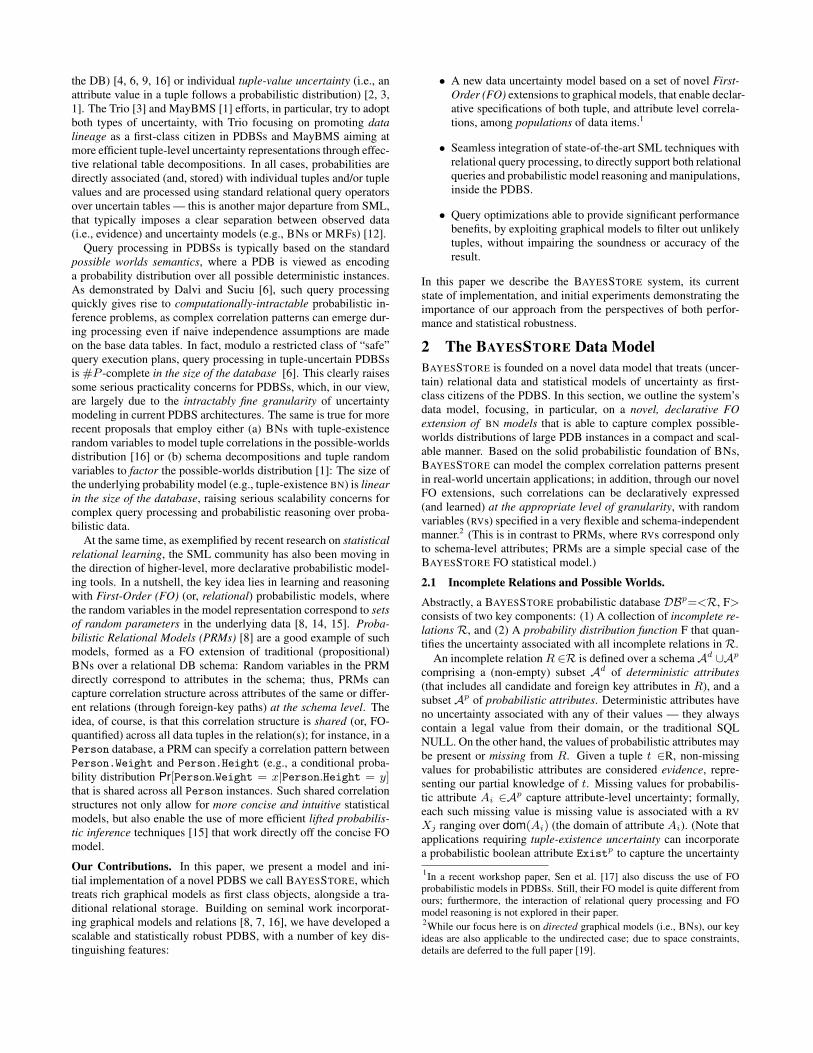
EXAMPLE 1. Suppose there are two sets of environmental sen-sors in different rooms of a hotel. The first set of sensors monitorstemperature and light levels; while the second monitors humidityand light levels. Sensor readings are inherently noisy – readingsmay be dropped due to sensor malfunctions or power fluctuations,or even garbled by radio interference from other equipment. Forthe ease of exposition, we assume that sensor readings are dis-cretized into binary values; Cold and Hot for temperature, Drk(Dark) andBrt (Bright) for light, andHigh andLow for humiditylevels. We regard all collected readings from the two sets of sen-sors being stored in a database DBpof two incomplete relations:Sensor1(Time(T), Room(R), Sid, tempp(Tp), lightp(L)), andSensor2(Time(T), Room(R), humidityp(H), lightp(L)), respectively.Probabilistic attributes are denoted with superscript p, while theattributes constituting the primary key are underlined. In this ex-ample, neither relation is associated with tuple-level existence un-certainty. Figure 1(a) depicts an instance of these relations. Blankcells correspond to missing values, and are represented by a RV foreach, taking values from the domain of the corresponding proba-bilistic attribute. Each RV can be referred to by its tuple identifierand attribute name (e.g. ε1.Tp is the RV of the missing value oftuple ε1). In this snapshot ofDBp, the possible worlds distribution

ε1.L ε1.Tp p

Brt Hot 0.8Drk Hot 0.2Drk Cold 0.8

Brt Cold 0.2

MBN: Bayesian Network

ε1.Tp

ε2.Lε2.Tp

ε1.L

CPT (ε1.L | ε1.Tp)

(a)

(b)Hot321

BrtDrk

Lp

221121

Cold311Cold211

111

TppSidRT

Incomplete Relation: Sensor1p

ε1ε2ε3ε4

ε5ε6

Incomplete Relation: Sensor2p

Drk

Lp

High2111

HpRT

ε1’ε2’

ε1

ε2

ε3

ε4

ε5

ε6

(b)

ε2’

ε1’

(c)

Figure 1: (a) Incomplete Relations Sensor1 and Sensor2. Eachtuple is referred to by its identifier (εi). (b) An exampleBayesian Network representation of the probabilistic distribu-tion of tuples ε1, ε2, and the CPT associated with RV ε1.L.(c) The mapping between the entity sets of two stripes, STp andSH , from Sensor1 and Sensor2 respectively, involved in a child-parent relationship.

F can be captured by an 8-dimensional distribution table, over the8 RVs associated with the uncertain quantities of the relations.

2.2 Bayesian Networks: A Quick Primer

Over the past 20 years, Bayesian Networks (BNs) have emerged asa widely-used SML model to efficiently represent and reason aboutmulti-variate probabilistic distributions [12]. A BN is a directedacyclic graph G = (V,E) with nodes representing a set of RVsX1, X2, . . . , X|V |, and edges denoting conditional dependencerelationships between RVs. In a nutshell, the structure of the BN en-codes the assertion that each node is conditionally independent ofits non-descendants, given its parents. This allows us to model theprobability distribution of a RV Xi, locally, as a Conditional Prob-ability Table (CPT) or factor Pr[Xi|Pa(Xi)] that specifies howXi

depends probabilistically on the values of its parent nodes Pa(Xi).It is not difficult to see that the overall joint probability distributioncan be factored into the product of all local models in the DAG; thatis, Pr[X1, ..., X|V |] =

Q|V |i=1 Pr[Xi|Pa(Xi)]. Given that the di-

mensionality of local correlation models is typically much smallerthan |V |, this factored BN representation can be orders of magni-tude more efficient than a straightforward |V |-dimensional proba-bility distribution.

Thus, a natural, first approach to compress the multi-variate dis-tribution F of a BAYESSTORE database DBp, is to encode it usinga BN: Every probabilistic attribute value in DBpis represented byone RV in the BN, and local CPT models capture probabilistic cor-relations across these values. Here, note that we are slightly gen-eralizing our earlier description of the BAYESSTORE probabilisticmodel by associating a RV with every probabilistic attribute value,either missing or not. Such a generalized model essentially ac-knowledges the potential for uncertainty in all probabilistic values,and is closer to the traditional SML point of view where models forall random quantities are learned from historical training quantitiesand further manipulated on the basis of current observations. In ad-dition, note that the required possible-worlds distribution functionF over just missing-value RVs can be obtained using conventionalSML techniques for conditioning the BN on the observed evidencevalues provided in the incomplete relations3.

3BNs can also accommodate continuous, or combinations of con-

Finally, we make a conceptual distinction between two types ofcorrelations (i.e., edges in the BN). A correlation involving RVsmapping to attribute values in the same tuple, is termed a hori-zontal correlation; otherwise (i.e., if the correlation associates RVsfrom distinct tuples), it is termed a vertical correlation. As we willsee, the distinction between the two is sometimes important duringquery processing in BAYESSTORE.

EXAMPLE 2. Figure 1(b) depicts a simple BN, representing thejoint Pr[ε1.Tp, ε1.L, ε2.Tp, ε2.L] of the 4 RVs that correspondto the probabilistic values of tuples ε1 and ε2. The local modelfor each RV is given by a conditional probability table (CPT). Thefigure shows only the CPT of RV ε1.L. The RV ε2.Tp is consid-ered an observed RV, as its value is fixed to Cold, from the evi-dence provided in Sensor1. The joint distribution F of Sensor1 canbe computed by calculating the probability Pr[ε1.Tp, ε1.L, ε2.L|ε2.Tp = Cold] over the BN. The edge between ε1.Tp and ε2.Tpconstitutes a vertical correlation; the rest are horizontal.

2.3 The BAYESSTORE FO Bayesian Network Model

Even with the use of a factored representation that exploits condi-tional independence among tuple variables, the size of the resultingtuple-based BN model (also referred to as a propositional BN) re-mains problematic: The model requires one RV per probabilisticattribute, per tuple, per relation! Such huge propositional BN mod-els are clearly not useful as an intuitive representation of the uncer-tainty in the data; furthermore, the cost of probabilistic reasoningover these models is bound to be prohibitive for non trivially-sizeddomains [16].

To overcome these problems, BAYESSTORE employs a novel re-finement of recent ideas in the area of First-Order (FO) probabilis-tic models [8, 14, 15]. More specifically, the BAYESSTORE prob-abilistic model is based on a novel class of First-Order BayesianNetwork (FOBN) models. In general, a FOBN model MFOBN

extends traditional (propositional) BN structures by capturing inde-pendence relationships between sets of RVs. This allows correlationstructures that are shared across multiple propositional RVs to becaptured in a concise manner. More formally, aMFOBN encodesa joint probability distribution by a set of FO factors MFOBN

= φ1, ..., φn — each such factor φi represents the local CPTmodel of a population of (propositional) RVs. For instance, thepopular Probabilistic Relational Models (PRMs) [8] are an instanceof FOBN models specified over a given relational schema: First-order RVs in a PRM directly correspond to schema attributes, andthe correlation structure specified is shared across all propositionalinstances in the relation (which are assumed to be independentacross tuples — i.e., no vertical correlations). Attributes in differ-ent relation schemas can also be correlated along key/foreign-keypaths [8].

The BAYESSTORE FOBN model is based on a non-trivial exten-sion to PRMs that allows correlation structure to be specified andshared across first-order RVs corresponding to arbitrary, declara-tively specified, sub-populations of tuples in a relational schema.Thus, unlike PRMs, shared correlation structures in BAYESSTOREcan be specified in a very flexible manner, without being tied to aspecific relational schema design. This flexibility can, in turn, en-able concise, intuitive representations of probabilistic information.The key, of course, is to ensure that such flexibly-defined FO cor-relation structures are also guaranteed to map to a valid probabilis-tic model over the base (propositional) RVs in the BAYESSTORE

tinuous and discrete RVs. In the interest of space, we restrict ourattention to discrete distributions, and refer the interested reader tostandard textbooks on the subject [5].

database. (Such a mapping is known as FO model “grounding” inthe SML literature.) In what follows, we give a brief overview ofsome of the key concepts underlying the BAYESSTORE FOBN un-certainty model, and how they ensure a valid mapping to a possible-worlds distribution.

First-Order RVs in BAYESSTORE: Entities, Entity Sets, andStripes. The following definition provides a declarative means ofspecifying arbitrary sub-populations of tuples by selecting “slices”of the deterministic part of an incomplete relation R.

DEFINITION 2.1. [Entity Set R.E ] An Entity Set (R.E) of anincomplete relation R with deterministic attributes K1, . . . ,Kn, isthe deterministic relation R.E (K′) (where K′ ⊆ K1, . . . ,Kn),defined as a relational algebra query which performs a selectionand a subsequent projection on any part K′ of K1, . . . ,Kn:R.E def

= πK′(σcondition onK′( R )).

The elements of an entity set essentially identify a number of“entities” at arbitrary granularities – tuples or tuple groups – whichcontain some probabilistic attributes that we intend to model. Notethat, in general, since entity sets are defined as projections on partsof R’s superkey, a particular entity ε can correspond to a set oftuples in R. The probabilistic attribute RV associated with ε corre-sponds, in fact, to the same RV across all R tuples correspondingto ε; in other words, in any possible world, a probabilistic attributeassociated with an entity is instantiated to the same value for all tu-ples in the entity’s extent. Thus, intuitively, entities define the gran-ularity of the base, propositional RVs in the BAYESSTORE model.An entity set then naturally specifies the granularity of first-orderRVs (quantified over all entities in the set).

Various entity sets can be specified for the same relation, de-pending on the level in which entities are captured. Among those,the maximal entity set of R, which associates an entity with eachtuple in R, can be obtained by projecting on any key of R— forour Sensor1 table example: Sensor1 .EM = πR,T,Sid(Sensor1 ).Each entity ε in Sensor1 .EM (i.e. each sensor reading tuple) is as-sociated with two uncertain quantities, its temperature (ε.Tp) andlight readings (ε.L), which can be represented by the RVs ε.XTp

and ε.XL, that model the stochastic process of assigning values toε.Tp and ε.L, respectively.

Coarser entity definitions are also useful when we need to asso-ciate the same RV for several tuples in an incomplete relation, i.e.,tuples that always have the same probabilistic attribute value in anypossible-world instantiation. Such situations arise naturally, for in-stance, when values of a probabilistic attribute are redundantly re-peated in a table or during the processing of cross-product and joinoperations over probabilistic attributes (Section 3.3).

Having specified the concept of entity sets, we can now naturallydefine the notion of first-order RVs in BAYESSTORE. Such FO RVs(termed stripes) represent the values of a probabilistic attribute fora population of entities that share the same probabilistic character-istics.

DEFINITION 2.2. [Stripe S <R.Ap, E >] A stripe S <R.Ap,E > over an entity set E of an incomplete relation R, represents aset of random variables, one per entity from E , which models thestochastic process of assigning values to the probabilistic attributeAp of that entity.

First-Order Factors and FOBNs in BAYESSTORE. As men-tioned earlier, a FO factor in a FOBN captures the shared cor-relation structure (CPT) for a group of underlying propositionalRVs (i.e., entities). Using our earlier definitions, we can define

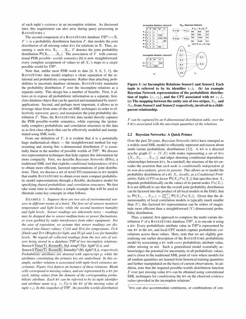
BAYESSTORE FO factor φ (S|Pa(S)), as a local CPT model thatdescribes the conditional dependence relationship between a childstripe S and its parent stripes Pa(S). For example, if for all en-tities in of the incomplete relation Sensor1 , the RV correspondingto light, Li, conditionally depends on the temperature, Tpi, of thesame entity εi (i.e., Tpi → Li), and this correlation pattern (i.e.,CPT) is shared across all entities, then this situation can be capturedconcisely by two stripes: STp =< Sensor.Tp, πR,T,SidSensor >and SL =< Sensor.L, πR,T,SidSensor >, and a FO factorover them: φ (SL|STp).

In the above example, we implicitly assumed the existence of aone-to-one mapping between entities in the child stripe (SL) andentities in its parent stripe (STp); i.e., each (propositional) RV Li ∈SL will have as a parent its corresponding Tpi ∈ STp. Althoughthis is often the case, non-bijective types of stripe mappings can bedefined as well.

DEFINITION 2.3. [Mapping between Stripes f [Sp, Sc]] A map-ping f between two stripes – a child stripe Sc < R.Ap

c , Ec > anda parent stripe Sp < R.Ap

p, Ep >, is a surjective function from theentity set Ec to Ep, f[Sp, Sc]: Ec → Ep, expressed as a first-orderlogic formula over the schemata Kc and Kp of the entity sets Ec

and Ep, whereKp ⊆ Kc. For the mapping to be valid, the selectionpredicates of the relational algebra expressions used to define Ec

and Ep respectively, need to be the same.

Definition 2.3 formalizes the association of the individual ele-ments (RVs) of two stripes involved in a “child-parent” relationship(Sp → Sc) at a per-instance level. In essence, it requires that everyRV from Sc will have a single corresponding parent RV from Sp. Inaddition, it ensures the minimality of the parent stripe Sp, throughthe constraint of surjectivity, as every RV in Sp has to be associatedwith at least one RV from Sc. From the above, while it is permis-sible for an RV from Sp to be parent of more than one RV fromSc, a child RV from Sc cannot have more than one parent (sincesuch multi-variable correlations cannot be captured by a single FOedge).

The last requirement of definition 2.3 essentially states that be-tween the entity set attributes of the child and the parent stripes,there is a key-foreign key relationship, so that the entities betweenthe two sets can be unambiguously associated with each other. Tocontinue the previous example, the “1-1” mapping between thestripe SL and its parent STp, can be expressed as:

(∀εL ∈ SL.E , ∀εTp ∈ STp.E)Pa(r.εL) = r.εTp, s.t.:εL.T = εTp.T ∧ εL.R = εTp.R ∧ εL.Sid = εTp.Sid

(1)

where r.εL signifies the RV associated with the entity εL fromstripe SL’s entity set, and Pa(r.εL) the parent RV of r.εL.

Up to this point we have tacitly assumed that we can expresscorrelations only among stripes of the same incomplete relation.Nevertheless, conditional dependence relationships can be formedbetween stripes of different relations. As noted earlier, the two rela-tions must be involved in a key-foreign key relationship, the foreignkey of the parent incomplete relation should be part of the primarykey of the child, and the selection predicates (if any), populatingthe entity sets of the stripes must be the same, for the last conditionof Definition 2.3 to be satisfied.

Following the running example of Figure 1, we assume that at-tributes T and R of Sensor form a foreign key for Sensor2. More-over, assume that for each room and timestamp, the temperaturereadings of the 3 different sensors in that room depend condition-ally on the (single) humidity reading for that timestamp (i.e., H →Tp), and that this correlation pattern is quantified by the same CPT

MFOBN: First-order Bayesian Network

S1:<Sensor1.Tp, T,R,Sid (σSid≠2 Sensor1)>

S2:<Sensor1,Tp, T,R,Sid Sensor1>

S3:<Sensor1.L, T,R,Sid Sensor1>

φ1 (S1):φ2 (S3|S2):

CPT2

CPT1S1 S2 S3

S5:<Sensor1.Tp,T,R,Sid (σSid=2 Sensor1)>

S4:<Sensor.Tp, T,R,Sid (σSid=1 Sensor1)>

φ3 (S5|S4):CPT3

S4 S5

Figure 2: First-order Bayesian Network model over the incom-plete relation Sensor1 in Figure 1.

across all such groups of RVs. That can be expressed by defining2 stripes, STp =< Sensor.Tp, πR,T,SidSensor > for temper-ature and SH =< Sensor2.H, πR,TSensor2 > for humidity,and a first order factor φ(STp|SH) which is made explicit throughthe one-to-many mapping:

(∀εTp ∈ STp.E ,∀εH ∈ SH .E)Pa(r.εTp) = r.εH , s.t.εTp.T = εH .T ∧ εTp.R = εH .R

(2)

The mapping f [STp, SH ] is graphically depicted in Figure 1(c). Inthis example we can see the application of Definition 2.3 in its fullgenerality; each entity of the parent stripe SH is associated with its3 corresponding entities from the child stripe STp, which can beuniquely defined because of the key-foreign key relationships thatcharacterize the two entity sets.

We are now ready to formally define a first-order factor.

DEFINITION 2.4. [First-order Factor φ (Si,fi,CPT)] A first-order factor φ represents the conditional dependency of a childstripe Sc on a set of parent stripes Pa(Sc) = Sp1 , . . . , Spn,φ (Sc|π(Sc)). It consists of:

• A child stripe Sc and a (possibly empty) ordered list of parentstripes Sp1 , . . . , Spn.

• A (possibly empty) ordered list of stripe mappings fi[Sc,Spi ], (i = 1, . . . , n), each one associating the entities ofthe child stripe with those of the corresponding parent stripe.

• A conditional probability table (CPT), quantifying the com-mon local model, that holds for all the RV associations thatare defined by the set of mappings fi[Sc, Spi ], among theentities of the stripes involved, P (Sc|π(Sc)).

A BAYESSTORE FOBN modelMFOBN can now be defined asa set of first-order factors Φ = φ1, ..., φn, where each φi de-fines a local CPT model for the corresponding child stripe. Notethat our definitions of stripes and stripe mappings are sufficient toguarantee that each individual FO factor can be grounded to a validcollection of local CPTs over propositional RVs (entities). In thepresence of multiple FO factors (and possible connections acrossfactors), ensuring that the globalMFOBN model can be groundedto a valid probabilistic distribution over entities is a little trickier.More specifically, note that even distinct stripes in factors can over-lap (see Example 3 below), and additional structural constraintsmust be imposed on the model to guarantee grounding to an acyclicBN model. Due to space constraints, details are deferred to the fullversion [19] of this paper.

EXAMPLE 3. Figure 2 shows an exampleMFOBN for our sen-sornet probabilistic database. There are three first-order factors:

φ1, φ2, φ3. For φ1, the child stripe φ1.S1 is defined over the at-tribute Tpp, and with an entity set of all the entities with Sid 6= 2.For φ2, both the child and parent stripes are defined over the maxi-mal entity set of the Sensor1 relation (i.e. for all tuples in Sensor1).Finally, for φ3, the child stripe is defined over the attribute Tpp ofall the entities with Sid = 2, and the parent stripe is defined overTpp of all the entities with Sid = 1. In all cases, “1-1” mappingfunctions are assumed, which along with the corresponding CPTs,are omitted from the figure in the interest of space.

Learning the shared correlation structure and the parameters ofa FO probabilistic model from data is known to be a challengingtask [18]. In an earlier workshop paper [13], we have discussed thecomplications of the learning process, and how it can be facilitatedover a hierarchical version of FOBNs. Developing a complete, ef-ficient learning solution for the BAYESSTORE FOBN model is inour immediate plans.

3 Query ProcessingHaving presented BAYESSTORE’s probabilistic model, in this sec-tion we consider basic query processing algorithms from the stan-dard SQL repertoire, namely selection, projection and join, ex-tended with inference operations over the incomplete relations ina probabilistic database DBp=< R, F >.

Unlike their relational counterparts, which operate only over de-terministic relations, operators over aDBphave to process both thedata in the incomplete relations and the possible-worlds distribu-tion. A naive approach to query processing is to perform tradi-tional relational operations on the set Ω of the exponentially manyworlds, to compute a new set of possible worlds Ω′, and correctlymap probabilities from F to F ’. Since this computation is clearlyintractable, the core challenge is to develop query execution tech-niques which, prior to operating on the data of DBp’s incompleterelations, manipulate the first-order model accordingly. This pre-processing step guarantees that the resulting probability distribu-tion F ’, encoded by the modified MFOBN , will be compatiblewith the new state of DBp.

3.1 SelectionWe focus our discussion on the use of a selection predicate %, thatis a conjunction of atomic predicates (% = ∧%i), whose operatorsinvolve arithmetic comparisons Θ ∈ <,>,6,>,= between aprobabilistic or deterministic attribute and a constant (% = AΘct).BAYESSTORE also supports other forms of atomic predicates, suchas % = ApΘBp (presented in Section 3.3, where probabilistic joinsare discussed), as well as boolean expressions involving disjunc-tions and negations, but details are omitted due to space restric-tions.

The techniques for performing selection over the model (as wecall the MFOBN modification process) which will be discussednext, have proven to be quite fundamental for all the relational op-erations described in this section. On the other hand, selection overthe tuples of R is not a trivial process either, as the filtering of theincompatible to % tuples is no longer deterministic. Section 3.1.2introduces a basic algorithm for selecting incomplete data tuples,as well as two optimizations, which attempt to reduce the size ofthe resulting incomplete relation R’, without affecting the validityof the selection output.

3.1.1 Selection over ModelMFOBN

In a deterministic DB, selection over a relation R reduces it to con-tain only the tuples that satisfy the selection predicate. Should Rbe an incomplete relation (e.g., the Sensor1 relation of Figure 1, inwhich some temperature and light readings are missing), a selection

with predicate % : (Sensor1 .Lp = Brt), apart from removing thetuples that have a light value different than Brt, affects the distri-bution of possible worlds F as well, since worlds where L = Drk

cannot be generated by %.In statistical model terms, this probabilistic selection operation

resembles that of computing the conditional distribution Pr[−→X |Y1 =

y1, . . . , Yn = yn] of a set of RVs−→X , given that RVs Yin1 ∈

−→X ,

have specific values y1, . . . , yn. Thus, it seems tempting to cal-culate the new possible-worlds distributionF ’ over the set of exam-ple RVs

−→XSensor = Tp1, . . . , Tpn, L1, . . . , Ln, by condition-

ing on all the RVs that correspond to Sensor1 .L = Brt. Unfortu-nately, this operation does not result in the correct possible worldsdistribution: In a nutshell, the problem here is that conditioning(and other standard model manipulations, such as marginalization)cannot by themselves express possible worlds with different num-bers of tuples — even under the conditioned/marginalized model,the number of tuples in each possible completion of an incompleterelation R is going to be the same (i.e., |R|). In contrast, apply-ing the selection operation over the possible worlds can obviouslyresult in worlds with different numbers of tuples, by filtering outtuples that do not satisfy the selection predicate; essentially, prob-abilistic selection introduces tuple-existence uncertainty (i.e., theexistence of a tuple in a possible world becomes uncertain).

Continuing with our example, a given tuple t ∈ Sensor1 appearsonly in the possible worlds where the attribute L = Brt, and inall the rest it is filtered out completely. On the other hand, by sim-ply calculating the conditional Pr[

−→XSensor|L1 = Brt, . . . , Ln =

Brt] directly over the model, the possible worlds correspondingto the resulting joint pdf all have the same number of tuples (i.e.,the number of tuples in Sensor1 with L 6= Drk) all having L =Brt. (It should also be intuitively clear that this (conjuctive) con-ditioning does not have the right semantics for our selection op-eration.) The fact that the cardinality of tuples between possibleworlds can vary cannot be directly expressed by standard condi-tioning/marginalization operations on the model.

We capture tuple existence uncertainty by introducing the prob-abilistic attribute Existp in the schema of the incomplete rela-tion being selected, if it is not contained already. Depending onwhether the selection predicate % involves a deterministic Ad, or aprobabilistic attributeAp, the corresponding selection over a modelσ(MFOBN ) behaves differently.

The atomic predicate % : (AdΘct), restricts the entity set towhich the predicate % applies. For example, % : (Sid = 3 ∧ Tp =Hot) restricts the entity set of predicate % to only include the enti-ties with Sid equals 3. Entities with Sid 6= 3 cannot exist in theresulting relation (i.e., their Existp=0).

Existence uncertainty is introduced in the model when % involvesa probabilistic attribute Ap. For example, if a predicate Tp = Hot

is applied to a tuple t with a missing Tp value, the presence of tin the output becomes probabilistically dependent on t.Tp’s value.Intuitively, this operation corresponds to changing the local modelof the factor that corresponds to R’s Existp attribute, to be depen-dent on that probabilistic attribute (for our example, Tp).

Figure 3 shows the select-model algorithm, based on a predi-cate % of the formAdΘ1ct1∧ApΘ2ct2. For example, % = (Sid =3 ∧ Tp = Hot). The algorithm can be easily extended to processa conjunctive predicate % with any number of atomic predicates.(Join predicates (e.g., AΘB) are discussed in Section 3.3.)

Lines 1-2 define the entity set on which the selection predicateapplies: %.E . The presence of the deterministic attribute inside %(Sid = 3) essentially restricts its entity set %.E (e.g., to all tupleswith Sid = 3); otherwise, the predicate applies to any entity within

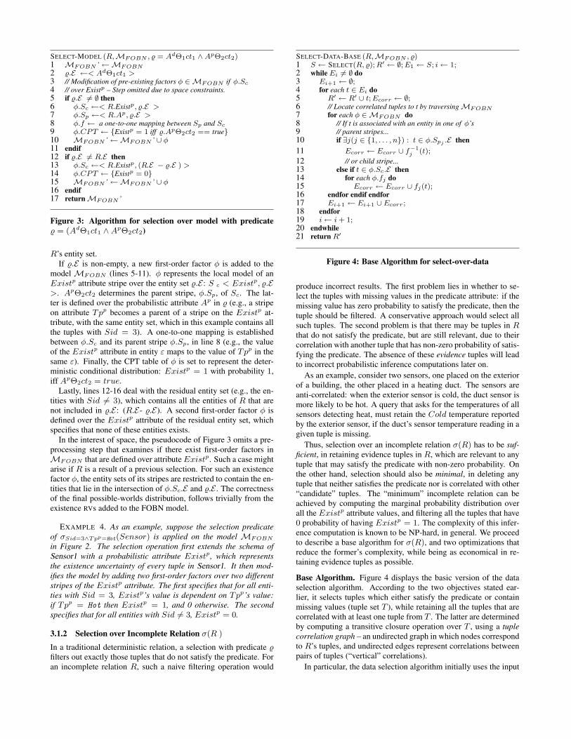
SELECT-MODEL (R,MFOBN , % = AdΘ1ct1 ∧ApΘ2ct2)1 MFOBN ’←MFOBN

2 %.E ←< AdΘ1ct1 >3 // Modification of pre-existing factors φ ∈MFOBN if φ.Sc

4 // over Existp – Step omitted due to space constraints.5 if %.E 6= ∅ then6 φ.Sc ←< R.Existp, %.E >7 φ.Sp ←< R.Ap, %.E >8 φ.f ← a one-to-one mapping between Sp and Sc

9 φ.CPT ← Existp = 1 iff %.ApΘ2ct2 == true10 MFOBN ’←MFOBN ’ ∪ φ11 endif12 if %.E 6= R.E then13 φ.Sc ←< R.Existp, (R.E − %.E ) >14 φ.CPT ← Existp = 015 MFOBN ’←MFOBN ’ ∪ φ16 endif17 returnMFOBN ’

Figure 3: Algorithm for selection over model with predicate% = (AdΘ1ct1 ∧ApΘ2ct2)

R’s entity set.If %.E is non-empty, a new first-order factor φ is added to the

model MFOBN (lines 5-11). φ represents the local model of anExistp attribute stripe over the entity set %.E : S c < Existp, %.E>. ApΘ2ct2 determines the parent stripe, φ.Sp, of Sc. The lat-ter is defined over the probabilistic attribute Ap in % (e.g., a stripeon attribute Tpp becomes a parent of a stripe on the Existp at-tribute, with the same entity set, which in this example contains allthe tuples with Sid = 3). A one-to-one mapping is establishedbetween φ.Sc and its parent stripe φ.Sp, in line 8 (e.g., the valueof the Existp attribute in entity ε maps to the value of Tpp in thesame ε). Finally, the CPT table of φ is set to represent the deter-ministic conditional distribution: Existp = 1 with probability 1,iff ApΘ2ct2 = true.

Lastly, lines 12-16 deal with the residual entity set (e.g., the en-tities with Sid 6= 3), which contains all the entities of R that arenot included in %.E : (R.E- %.E). A second first-order factor φ isdefined over the Existp attribute of the residual entity set, whichspecifies that none of these entities exists.

In the interest of space, the pseudocode of Figure 3 omits a pre-processing step that examines if there exist first-order factors inMFOBN that are defined over attributeExistp. Such a case mightarise if R is a result of a previous selection. For such an existencefactor φ, the entity sets of its stripes are restricted to contain the en-tities that lie in the intersection of φ.Sc.E and %.E . The correctnessof the final possible-worlds distribution, follows trivially from theexistence RVs added to the FOBN model.

EXAMPLE 4. As an example, suppose the selection predicateof σSid=3∧Tpp=Hot(Sensor) is applied on the model MFOBN

in Figure 2. The selection operation first extends the schema ofSensor1 with a probabilistic attribute Existp, which representsthe existence uncertainty of every tuple in Sensor1. It then mod-ifies the model by adding two first-order factors over two differentstripes of the Existp attribute. The first specifies that for all enti-ties with Sid = 3, Existp’s value is dependent on Tpp’s value:if Tpp = Hot then Existp = 1, and 0 otherwise. The secondspecifies that for all entities with Sid 6= 3, Existp = 0.

3.1.2 Selection over Incomplete Relation σ(R )

In a traditional deterministic relation, a selection with predicate %filters out exactly those tuples that do not satisfy the predicate. Foran incomplete relation R, such a naive filtering operation would

SELECT-DATA-BASE (R,MFOBN , %)1 S ← SELECT(R, %);R′ ← ∅;E1 ← S; i← 1;2 while Ei 6= ∅ do3 Ei+1 ← ∅;4 for each t ∈ Ei do5 R′ ← R′ ∪ t;Ecorr ← ∅;6 // Locate correlated tuples to t by traversingMFOBN

7 for each φ ∈MFOBN do8 // If t is associated with an entity in one of φ’s9 // parent stripes...10 if ∃j(j ∈ 1, . . . , n) : t ∈ φ.Spj .E then11 Ecorr ← Ecorr ∪ f−1

j (t);

12 // or child stripe...13 else if t ∈ φ.Sc.E then14 for each φ.fj do15 Ecorr ← Ecorr ∪ fj(t);16 endfor endif endfor17 Ei+1 ← Ei+1 ∪ Ecorr;18 endfor19 i← i+ 1;20 endwhile21 return R′

Figure 4: Base Algorithm for select-over-data

produce incorrect results. The first problem lies in whether to se-lect the tuples with missing values in the predicate attribute: if themissing value has zero probability to satisfy the predicate, then thetuple should be filtered. A conservative approach would select allsuch tuples. The second problem is that there may be tuples in Rthat do not satisfy the predicate, but are still relevant, due to theircorrelation with another tuple that has non-zero probability of satis-fying the predicate. The absence of these evidence tuples will leadto incorrect probabilistic inference computations later on.

As an example, consider two sensors, one placed on the exteriorof a building, the other placed in a heating duct. The sensors areanti-correlated: when the exterior sensor is cold, the duct sensor ismore likely to be hot. A query that asks for the temperatures of allsensors detecting heat, must retain the Cold temperature reportedby the exterior sensor, if the duct’s sensor temperature reading in agiven tuple is missing.

Thus, selection over an incomplete relation σ(R) has to be suf-ficient, in retaining evidence tuples in R, which are relevant to anytuple that may satisfy the predicate with non-zero probability. Onthe other hand, selection should also be minimal, in deleting anytuple that neither satisfies the predicate nor is correlated with other“candidate” tuples. The “minimum” incomplete relation can beachieved by computing the marginal probability distribution overall the Existp attribute values, and filtering all the tuples that have0 probability of having Existp = 1. The complexity of this infer-ence computation is known to be NP-hard, in general. We proceedto describe a base algorithm for σ(R), and two optimizations thatreduce the former’s complexity, while being as economical in re-taining evidence tuples as possible.

Base Algorithm. Figure 4 displays the basic version of the dataselection algorithm. According to the two objectives stated ear-lier, it selects tuples which either satisfy the predicate or containmissing values (tuple set T ), while retaining all the tuples that arecorrelated with at least one tuple from T . The latter are determinedby computing a transitive closure operation over T , using a tuplecorrelation graph – an undirected graph in which nodes correspondto R’s tuples, and undirected edges represent correlations betweenpairs of tuples (“vertical” correlations).

In particular, the data selection algorithm initially uses the input

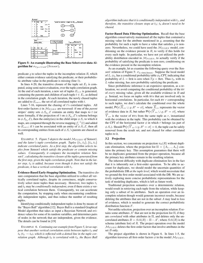
Figure 5: An example illustrating the Base Select-over-data Al-gorithm for σTp=‘Cold′(Sensor).

predicate % to select the tuples in the incomplete relation R, whicheither contain evidence satisfying the predicate, or their probabilis-tic attribute value in the predicate is missing (line 1).

In lines 4-20, the transitive closure of the tuple set E1 is com-puted, using semi-naive evaluation, over the tuple correlation graph.At the end of each iteration, a new set of tuples Ei+1 is generated,containing the parents and children of each tuple t ∈ Ei, as definedin the correlation graph. At each iteration, the newly chased tuplesare added to Ecorr , the set of all correlated tuples with t.

Lines 7-16, represent the chasing of t’s correlated tuples. Allfirst-order factors φ inMFOBN are traversed: if one of the parentstripes’ entity sets φ.Spj .E contains an entity that maps to t (ormore formally, if the projection of t on φ.Spj .E’s schema belongsin φ.Spj .E), then the entity(ies) in the child stripe φ.Sc to which itmaps, are computed through the reverse mapping f−1

j (t) and addedto Ecorr; if t can be associated with an entity of φ.Sc.E , then allits corresponding entities from each of φ.Sc’s parents are chased aswell.

EXAMPLE 5. Figure 5 depicts the modelMFOBN of Sensor1,and the latter’s tuple correlation graph. Tuples t1, t2, t4, t5indicate correlated pairs. As a first step, the algorithm selects tu-ples from Sensor1 which satisfy the predicate or contain missingvalues. Consequently, it computes the incomplete relation Sen-sor1’, calculating the transitive closure of the tuples generated fromthe first step, given the tuple correlation graph. Note that in the lat-ter step, t2 is added, because even though it does not satisfy thepredicate, it has a vertical correlation with t1.

Evidence-Based Early-Stopping Optimization. The transitive clo-sure computation that the base algorithm utilized to collect all ver-tically correlated tuples, despite its correctness, might conserva-tively select more tuples than necessary. However, two tuples t1and t2 may be conditionally independent, even if there exists a ver-tical correlation between them. Consequently, we can acceleratethe computation, by stopping early when encountering condition-ally independent tuples, and thus reduce the number of resultingtuples.

Identifying conditionally independent tuples is done by means ofthe “Bayes Ball” algorithm [12]. Bayes Ball is a standard GraphicalModel algorithm that takes as input a Bayesian Network and evi-dence values for some of its random variables, and determines pairsof nodes in the network that are independent, given the evidence.The details can be found in [19]

EXAMPLE 6. Continuing our example from Figure 5, let us sup-pose that another vertical correlation exists between tuples t2 andt6 (t2 → t6), which is reflected with a dotted line in the tuple cor-relation graph. Although t6 is correlated with t2, the Bayes Ball

algorithm indicates that it is conditionally independent with t1, andtherefore, the transitive closure stops at t2; t6 doesn’t need to bechased.

Factor-Based Data Filtering Optimization. Recall that the basealgorithm conservatively maintained all the tuples that contained amissing value for the attribute mentioned in %, assuming that theprobability for such a tuple to have a value that satisfies % is non-zero. Nevertheless, we could have used theMFOBN model, con-ditioning on the evidence present in R, to verify if this holds forevery such tuple. In particular, we have not yet utilized the prob-ability distribution encoded in MFOBN , to actually verify if theprobability of satisfying the predicate is non-zero, conditioning onthe evidence present in the incomplete relation.

As an example, let us examine the following query over the Sen-sor1 relation of Figure 5: σL=Drk(Sensor). Suppose the local modelof L, φ2, has a conditional probability table φ2.CPT, indicating thatprobability of L = Drk is zero when Tp = Hot. Thus t2, with itsL value missing, has zero probability satisfying the predicate.

Since probabilistic inference is an expensive operation, as a re-laxation, we avoid computing the conditional probability of the RVof every missing value, given all the available evidence in R and%. Instead, we focus on tuples with RVs that are involved only inhorizontal correlations. In particular, for each RV r correspondingto such tuples, we don’t calculate the conditional over the wholemodel, Pr[r|

−→X ev ∪ %.Ap = ct], where

−→X ev represents the vector

of evidence data in R, but rather Pr[r|−→Y ev ∪ %.Ap = ct], where

−→Y ev is the vector of RVs from the same tuple as r, instantiatedwith the evidence in the tuple. This probability can be obtained bythe CPT of the horizontal factor φ in which r belongs (as part ofφ.Sc). Should Pr[r|

−→Y ev ∪%.Ap = ct] = 0, the tuple can be safely

removed from the result set, and not chased for other correlatedtuples to it.

3.2 ProjectionIn this section, we concentrate on projection πΠ(R) without dupli-cate elimination, where the projection list Π = A1, .., An con-tains the primary key. This assumption guarantees that there willbe no duplicates generated from the project operation, because allthe primary key attributes remain in the resulting relation.

The inherent difficulty with duplicate elimination lies in the factthat it is inherently not a first-order operation. To be able to ac-count for duplicates, we should model the uncertain quantities ofthe probabilistic DB at the tuple level, which would necessitate thatwe ground the first order model associated with the DB. We are ac-tively exploring more concise probabilistic representations for thetask of modeling duplicates, which is left as future work.

Traditional projection semantics over a deterministic relation,would result in retrieving each tuple from the relation, while keep-ing only a subset of its attributes. Such an operation over an in-complete relation though would generate incorrect results, becausedeleting the attributes that are not in the subset A may lead to lossof evidence, which is needed to generate the correct probabilisticdistribution function F .

Not unlike selection, projection over an incomplete relationR re-tains some attributes A∗ that are not in the projection list Π, if theyare correlated with other attributes in Π, and deletes only the un-correlated attributesB = Sch(R)−Π−A∗, where Sch(R) is theschema (attribute list) of R. The project operation over the modelMFOBN deletes the first-order factors that involve attributes in theset B only.

The project algorithm is shown in Figure 6. In lines 1-5, thealgorithm traverses all first-order factors φ in the modelMFOBN .

PROJECT (R,MFOBN ,Π)1 MFOBN ’←MFOBN

2 for each φ ∈MFOBN do3 if ∃i, j : φ.Si.A

p ∈ Π && φ.Sj .Bp /∈ Π then

4 Π← Π ∪Bp

5 endif endfor6 for each φ ∈MFOBN do7 if ∀i, φ.Si.A

p /∈ Π then8 MFOBN ’←MFOBN ’− φ;9 endif endfor10 R′ ← ∅11 for each t ∈ R do12 R′ ← R′ ∪ t(Π)13 endfor14 returnR′,MFOBN ’

Figure 6: Projection algorithm over Incomplete Relations

If φ involves two attributes Ap and Bp, where Ap belongs in theproject list (Ap ∈ Π), and Bp does not (Bp /∈ Π), then Ap and Bp

are correlated by factor φ. Thus, on line 3, the algorithm retainsBp in project attribute set Π. In lines 6-9, the algorithm traversesall the first-order factors a second time, and processes the modelMFOBN ’ to remove first-order factors that only involve attributeswhich are not in the newly computed set Π. In lines 11-13, thealgorithm iterates through every tuple in the incomplete relationR,and performs a traditional projection of each tuple on the attributesthat remained in Π.

EXAMPLE 7. Using the example in Figure 5, suppose we havea new probabilistic attribute Humidity H , and a new first-orderfactor φ4, which represents a prior probability table for all at-tribute values in H . Suppose we are to perform the projectionπT,R,Sid,L on this modified incomplete relation Sensor1. Sincethe first-order factor φ2 encodes a correlation between attributesTp and L, Tp is then included in the projection attribute set Π. At-tributeH is not included in Π, because it is not correlated with anyattribute in Π. Thus, the model of Sensor1 is modified by deletingφ4, because it only involves attribute H . Finally, the new incom-plete relation is generated by projecting every tuple of Sensor1 onthe subset of attributes Π = T,R, Sid, Tp, L.

3.3 JoinWe now turn our attention on binary selection predicates. In par-ticular, we will examine how the join operator (./%) between twoincomplete relations R1 and R2, whose entities’ correlation pat-terns are captured by the first order model MFOBN , determinesthe contents of the resulting incomplete relation R = R1 ./% R2,as well as the necessary modifications toMFOBN . We will con-centrate on join predicates of the form: % = (R1.A

pΘR2.Bp),

where attributes A and B are probabilistic.

3.3.1 Join over ModelMFOBN

The modifications toMFOBN which are required to maintain theconsistency of the probability distribution F with respect to R, arequite similar to those that the selection over the model algorithmperforms. As in Section 3.1.1, we need to capture the existence un-certainty of every joinable pair of tuples r1 ∈ R1 and r2 ∈ R2, inthe final result. The possible universe of these pairs corresponds toR1×R2. Nevertheless, these possibilities are restricted by the joinpredicate %. Hence, the challenge, as in selection, lies in capturingthe existence uncertainty of all probable tuple pair combinations ina first order fashion.

To accomplish this, we extendMFOBN by adding a first-orderfactor overR.Existp, which depends on the probabilistic attributes

JOIN (R1(K, . . . , Ap), R2(K′, . . . , Bp),MFOBN , %)

1 R← R1 ./% R2;2 %.E ← π

K∪K′ (R1 ×R2)

3 // Assign unique names to the stripes of the factors inMFOBN

4 for each φ ∈MFOBN do5 φ.Sc ← RENAME(φ.Sc, Sch(R))6 for each parent stripe φ.Spi , i = 1, . . . , n do7 φ.Spi ← RENAME(φ.Spi , Sch(R))8 endfor endfor910 // Create an existence factor11 φ.Sc ←< R.Existp, %.E >12 φ.Sp1 ←< R1.Ap, R1.E >13 φ.Sp2 ←< R2.Bp, R2.E >14 φ.f1 ← ∀εc ∈ φ.Sc.E , ∃ε1 ∈ φ.Sp1 .E , φ.f1(εc) = ε1 : εc.K = ε1.K

15 φ.f2 ← ∀εc ∈ φ.Sc.E , ∃ε2 ∈ φ.Sp2 .E , φ.f2(εc) = ε2 : εc.K′

= ε2.K′

16 φ.CPT ← Existp = 1 iff % == true17 M′FOBN ←MFOBN ∪ φ18 return R,M′FOBN

Figure 7: Join algorithm over ModelMFOBN .

Ap and Bp that participate in %. The algorithm is described in Fig-ure 7. Initially, as a preprocessing step (lines 4–8), we rename theattributes in the schema of R, Sch(R), to be able to refer to eachattribute of R by a unique name. This renaming step needs to becarried over the attributes of the stripes of each first-order factor inMFOBN as well, so that the correspondence ofMFOBN ’s stripeswith the probabilistic attributes of R is maintained.

Lines 10–17 define the new existence first-order factor φ. Essen-tially, the entity set of φ’s child stripe, φ.Sc.E corresponds to thecross product of the entities of the relations to be joined,R1(K, . . . , Ap)

and R2(K, . . . , Bp), where K and K′

are the sets of attributescomprising the primary keys of R1 and R2 respectively, as indi-cated by line 2. φ.Sc’s parents are the stripes φ.Sp1 and φ.Sp2 ,representing the populations of RVs for the join attributes R1.A

p

andR1.Bp. Each entity εc from φ.Sc.E is associated with the orig-

inal “copies” of the two entities, ε1 and ε2, from which it was gen-erated – one from each respective parent stripe. This many-to-oneassociation between an entity of one of the two initial relations, andits multiple copies in the entity set of φ.Sc, is captured by the map-ping functions φ.f1 and φ.f2 (lines 14–15). Finally, the CPT ofthis new factor represents the deterministic conditional distributionExistp = 1 with probability 1, iff R1.A

pΘR2.Bp = true.

As a special case, if R1 or R2 are a result of a previous selec-tion, in which caseMFOBN contains existence factor(s) already,a similar process takes place, which extends the entity sets of thechild and parent stripes involved, as well as the condition definingthe factors’ CPTs, to the resulting cross-product domain of the join.A detailed description of this special case can be found in the fullversion of the paper, [19].

3.3.2 Joining Incomplete Relations

As in the case of selection, the presence of missing values for theprobabilistic attributes of an incomplete relation, causes compli-cations when the latter is to participate in a join. In particular,when the attributes participating in a join predicate are probabilistic(R1.A

pΘR2.Bp), each tuple of R1 (equivalently for R2) that has

a missing value for Ap, may satisfy % and thus participate in thejoin result, depending on the possible values it can take, accordingto theMFOBN and the evidence present in R1 and R2. Followingthe same intuition as in section 3.1.2, all such tuples from both re-lations should be considered “joinable” conservatively, as the joinoperation per se becomes uncertain.

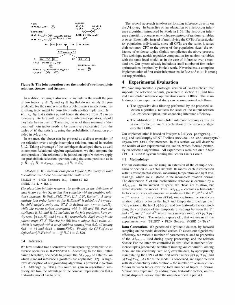
Figure 8: The join operation over the model of two incompleterelations, Sensor1 and Sensor2.

In addition, we might also need to include in the result the joinof two tuples r1 ∈ R1 and r2 ∈ R2 that do not satisfy the joinpredicate, for the same reason this problem arises in selection; thisresulting tuple might be correlated with another tuple from R =R1 ./% R2 that satisfies %, and hence its absence from R can er-roneously interfere with probabilistic inference operators, shouldthey later be run over it. Therefore, the set of these seemingly “dis-qualified” join tuples needs to be transitively calculated from thetuples of R′ that satisfy %, using the probabilistic information pro-vided inMFOBN .

In essence, the above can be phrased as a direct extension ofthe selection over a single incomplete relation, studied in section3.1.2. Taking advantage of the techniques developed there, as wellas common Relational Algebra equivalences, we first compute thecross product of the relations to be joined, on top of which we applyour probabilistic selection operator, using the same predicate as in%: R1 ./% R2 = σ%=(R1.AΘR2.B)(R1 ×R2).

EXAMPLE 8. Given the example in Figure 8, the query we wantto evaluate over these two incomplete relations is:SELECT * FROM Sensor1 R1, Sensor2 R2

WHERE R1.L = R2.L

The algorithm initially renames the attributes in the definition ofeach factor’s stripe Si, so that they coincide with the resulting rela-tion’s schema: R(Sid1, Sid2, Tpp, L1p, L2p, Existp). A deter-ministic first-order factor φ4 for R.Existp is added toMFOBN .Its child stripe’s entity set, S7.E is defined as: πSid1,Sid2R,while the parent stripes associated with it, S5 and S6, over theattributes R.L1 and R.L2 included in the join predicate, have en-tity sets: πSid1R and πSid2R respectively. Each entity in theparent stripe S5.E (likewise for S6) has a unique Sid1 value, s1,which is mapped with a set of children entities from S.E , all havingSid1 = s1 and Sid2 ∈ dom(Sid2). Finally, the CPT of φ4 isdefined as:(R.Existp = 1, iff R.L1 = R.L2).

3.4 Inference

We have studied two alternatives for incorporating probabilistic in-ference operators in BAYESSTORE. According to the first, rathernaive alternative, one needs to ground theMFOBN to a flat BN, onwhich standard inference algorithms are applicable [12]. A high-level description of our grounding algorithm is provided in Section2.3. Although by taking this route we gain in algorithmic sim-plicity, we lose the advantage of the compact representation that afirst-order model has to offer.

The second approach involves performing inference directly ontheMFOBN . Its basis lies on an adaptation of a first-order infer-ence algorithm, introduced by Poole in [15]. The first-order infer-ence algorithm, operates on whole populations of random variablesat once. Essentially, instead of multiplying the CPTs of a particularRV population individually, since all CPTs are the same, it raisestheir common CPT to the power of the population sizes; the ex-istence of evidence tuples slightly complicates the above process.This technique avoids repetitive computation for random variableswith the same local model, as in the case of inference over a stan-dard BN. Our system already includes a small number of first-orderoptimizations, inspired by Poole’s work. Nevertheless, a completeimplementation of first-order inference inside BAYESSTORE is amongour top priorities.

4 Experimental EvaluationWe have implemented a prototype version of BAYESSTORE thatsupports the selection variants, presented in section 3.1, and lim-ited First-Order inference optimizations over FOBNs. The mainfindings of our experimental study can be summarized as follows:

• The aggressive data filtering performed by the proposed se-lection algorithms, reduces the sizes of the output relation(i.e., evidence tuples), thus enhancing inference efficiency.

• The utilization of First-Order inference techniques resultsin even further, dramatic acceleration of the inference stageover the FOBN.

Our implementation is based on Postgres 8.2.4 (www.postgresql.-org) and uses Murphy’s BNT Toolbox (www.cs.ubc.ca/∼murphyk/-Bayes/bnt.html) for inference. In this section we will describethe results of our experimental evaluation, which focused primar-ily on selection algorithms. All experiments were run on a 2.8GzCPU, 1GB RAM system running the Fedora Linux Core 5.

4.1 MethodologyFor our evaluation we are using an extension of the example sce-nario of Section 2 – a hotel DB with 10 rooms, each instrumentedwith 8 environmental sensors, measuring temperature and light levelreadings, which are all stored in the incomplete relation Sensor.The distribution F of this probabilistic database is captured by aMFOBN . In the interest of space, we chose not to show, butrather describe the model. Thus, MFOBN contains 4 first-orderfactors: a prior for all temperature readings of the 1st, 3rd and 5th

– 8th sensor for every room φ(Tp), one capturing the same cor-relation pattern between the light and temperature readings overevery sensor in the hotel φ(L|Tp), and two first-order factors mod-eling the correlation of the temperature readings between the 1st

and 2nd, and 3rd and 4th sensor pairs in every room, φ(Tp2|Tp1)and φ(Tp4|Tp3). The selection query Q1, that we use in all theexperiments, was: ‘SELECT * FROM Sensor WHERE L=’Drk’’.

Data Generation. We generated a synthetic dataset, by forwardsampling on the model described earlier. To assess our algorithms’efficiency, we varied a number of parameters related to propertiesof the MFOBN used during query processing, and the relationSensor. For the latter, we controlled its size ‘size’ in number of ev-idence tuples generated, the ratio of missing values ‘mratio’ amongthem, and the selectivity ‘sel ’ of Q over the data, by appropriatelymanipulating the CPTs of the first order factors φ(Tp2|Tp1) andφ(Tp4|Tp3). As far as the model is concerned, we experimentedwith its connectivity ratio ‘cratio’ – the number of vertical corre-lations between tuples over the total number of tuples in Sensor.‘cratio’ was expressed by adding more first-order factors, on dif-ferent stripes of Sensor, than the ones described in par. 4.1.

Execution TimeSELECT * FROM Sensor WHERE L='Dark' INFER joint-distr

0

10

20

30

40

50

60

NaiveSel PlainSel FactorSel EvidenceSel FullSel

time(

sec)

Inference Inference with First-order Sharing

Figure 10: Inference execution time for query Q′. size =10000,sel =0.01, cratio =7/8, mratio =0.01.

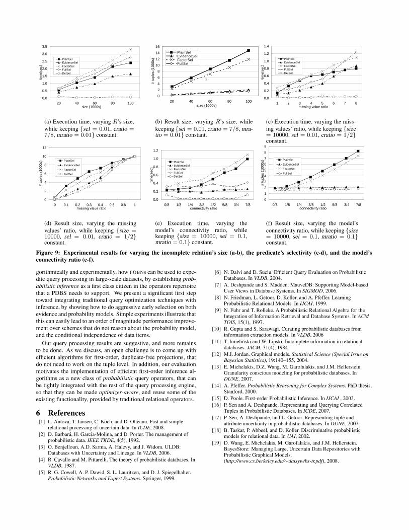
Algorithms and Metrics. In this section, we present our experi-mental setting, which includes four selection algorithms over in-complete relations, incorporating the optimizations presented inSection 3.1.2. Algorithm PlainSel filters data tuples of an incom-plete relation R using the traditional selection operator, and gener-ates evidence tuples, resorting to full transitive closure over R andthe model structure. EvidenceSel uses the “evidence-based early-stopping” technique on top of PlainSel, while FactorSel ex-tends PlainSel by incorporating the “factor-based early-stopping”technique. Lastly, FullSeluses both optimizations.

We also use two baseline algorithms; NaiveSel, which keeps alltuples in the incomplete relation as evidence, and DetSel, whichapplies a traditional over R. As we argued in Section 3, DetSelwill not produce correct answers. Nevertheless, we included it inour experimentation to compare its execution time (expected to bethe smallest) against the proposed algorithms.

4.2 Scalability

In this first experiment, we varied the size of Sensor, while keep-ing the selectivity (0.01), the connectivity (7/8), and the ‘mratio’(0.01) constant. Because “evidence-based early-stopping” reducesthe cost of the transitive closure computation and the size of theresult relation, EvidenceSel and FullSel have shorter executiontimes (as in Fig. 9(a)) and smaller result sizes (as in Fig. 9(b)) thanthe PlainSel and FactorSel variants. By comparing FactorSeland PlainSel, we observe that the “factor-based data-filtering”technique employed by the former decreases the result size, but itincreases the execution time. As expected, DetSel, has always thelowest cost, yet producing incorrect results.

4.3 Data Uncertainty

We also experimented by varying the ratio of missing values ‘mra-tio’ in Sensor, while keeping its size to 10000 tuples, Q’s selec-tivity to 0.01, and MFOBN ’s connectivity ratio to 0.5. As indi-cated in Fig. 9(c), the execution time of the algorithms utilizingthe “evidence-based early-stopping” technique grows more rapidlythan the rest, as ‘mratio’ increases. This behavior is justifiable,as a higher number of missing values indicates less evidence onwhich these algorithms can be based. Thus, on the higher end ofthe spectrum, EvidenceSel proves to be more expensive than theNaiveSel, and likewise FullSel is more expensive than FactorSel.

4.4 Model’s Connectivity Ratio

The third parameter we varied was the model’s connectivity ratio,keeping this time Sensor’s size (10000) and ‘mratio’ (0.1), andQ’sselectivity (0.1) constant. Figures 9(e) and 9(f) clearly demonstratethat the execution time and the result relation’s size of PlainSeland FactorSel increase linearly with respect to connectivity, be-cause they do not utilize the “evidence-based early-stopping” tech-

nique. On the other hand, ‘cratio’ of the model has little effect onEvidenceSel and FullSel, with a minimal increase in the resultsize of around 10%.

4.5 Inference

One of BAYESSTORE’s major objectives is the integration of rela-tional queries with probabilistic inference operators. In our finalexperiment, we make use of an SQL extension which computesthe joint distribution F of the RVs that correspond to the miss-ing values of Sensor, for all the readings that satisfy the conditionL=’Drk’. A presentation of our proposed SQL extension can befound in the extended version of our paper. Thus, we are execut-ing the query Q′: ‘SELECT * FROM Sensor WHERE L=’Dark’

INFER joint-distr’, which according to our query semantics,will produce a new incomplete relation Sensor’ and modelMFOBN ’.

The selection of Q′ operates both on the modelMFOBN , usingthe Select-Model algorithm of paragraph 3.1.1, and on Sensor,using the different data selection algorithms of our experimentalframework. The resulting model MFOBN ’ is grounded to a flatBayesian Network, so that standard inference algorithms can beapplied. Due to time limitations, rather than integrating an infer-ence operator in our prototype, we used the implementation of theVariable Elimination algorithm from Kevin Murphy’s BNT tool-box. On top of it, as we briefly describe in Section 3.4, we im-plemented one of the First-Order inference techniques discussedin [15] (FirstorderSharing technique), which allow us to sharethe inference computation over a population of instances with thesame model template, without fully grounding the model. Supposea sensor deployment, where every sensor has an independent andidentical probabilistic model. The inference computation is identi-cal, and thus can be shared among all sensor readings with the sameprobabilistic attribute values.

Fig. 10 shows the total execution time of Q′, using our vari-ous data selection algorithms, with and without our first-order op-timizations. The latter result to reduction on the query executiontime. The execution time decreases as we apply more complicatedoptimizations in the selection algorithm. With FirstorderSharing,NaiveSel, which keeps the full incomplete relation as evidence,takes the most processing time. FullSel completes in only halfthe time, compared to NaiveSel. The decrease is more dramaticwithout first-order optimization. These results indicate that dataand evidence filtering techniques manage to reduce the time of theinference operator, as a welcome effect of the incomplete relation’ssize reduction. The increased cost for the select operation is almostten times less than the reduced cost for the inference operation.

5 Conclusions and Future WorkIn this paper we presented BAYESSTORE, a Probabilistic DatabaseSystem that draws results from the Statistical Learning literature, toefficiently express and reason about correlations among uncertaindata items, in a concise and statistically sound way. BAYESSTOREis based on a novel data model, comprised of a set of IncompleteRelations and a probability distribution over those relations. Thus,our PDBS manages to fully expose both the incomplete relationsand their distribution to the user, as a unified, robust probabilis-tic representation that can be jointly manipulated. Furthermore, itrepresents one of the first successful attempts to seamlessly inte-grate state of the art Statistical Machine Learning techniques withrelational query processing.

To represent probability distributions compactly, we use First-Order Bayesian Networks (FOBNs), which use a small set of first-order factors to capture correlation patterns between entire popula-tions of uncertain entities. Furthermore, we have illustrated both al-

0.0

0.5

1.0

1.5

2.0

2.5

3.0

3.5

20 40 60 80 100size (1000s)

time(

sec)

PlainSelEvidenceSelFactorSelFullSelDetSel

(a) Execution time, varying R’s size,while keeping sel = 0.01, cratio =7/8, mratio = 0.01 constant.

0

2

4

6

8

10

12

14

16

20 40 60 80 100size (1000s)

# tu

ples

(100

0s)

PlainSelEvidenceSelFactorSelFullSel

x

(b) Result size, varying R’s size, whilekeeping sel = 0.01, cratio = 7/8, mra-tio = 0.01 constant.

0.0

0.2

0.4

0.6

0.8

1.0

1.2

1.4

1 2 3 4 5 6 7 8missing value ratio

time(

sec)

PlainSelEvidenceSelFactorSelFullSelDetSel

(c) Execution time, varying the miss-ing values’ ratio, while keeping size= 10000, sel = 0.01, cratio = 1/2constant.

0

2

4

6

8

10

12

0 0.1 0.2 0.3 0.4 0.6 0.8 1missing value ratio

# tu

ples

(100

0s) PlainSel

EvidenceSelFactorSelFullSel

(d) Result size, varying the missingvalues’ ratio, while keeping size =10000, sel = 0.01, cratio = 1/2constant.

0.0

0.2

0.4

0.6

0.8

1.0

1.2

0/8 1/8 1/4 3/8 1/2 5/8 3/4 7/8connectivity ratio

time(

sec)

PlainSelEvidenceSelFactorSelFullSelDetSel

(e) Execution time, varying themodel’s connectivity ratio, whilekeeping size = 10000, sel = 0.1,mratio = 0.1 constant.

0123456789

0/8 1/8 1/4 3/8 1/2 5/8 3/4 7/8connectivity ratio

# tu

ples

(100

0s) PlainSel

EvidenceSelFactorSelFullSel

(f) Result size, varying the model’sconnectivity ratio, while keeping size= 10000, sel = 0.1, mratio = 0.1constant.

Figure 9: Experimental results for varying the incomplete relation’s size (a-b), the predicate’s selectivity (c-d), and the model’sconnectivity ratio (e-f).

gorithmically and experimentally, how FOBNs can be used to expe-dite query processing in large-scale datasets, by establishing prob-abilistic inference as a first class citizen in the operators repertoirethat a PDBS needs to support. We present a significant first steptoward integrating traditional query optimization techniques withinference, by showing how to do aggressive early selection on bothevidence and probability models. Simple experiments illustrate thatthis can easily lead to an order of magnitude performance improve-ment over schemes that do not reason about the probability model,and the conditional independence of data items.

Our query processing results are suggestive, and more remainsto be done. As we discuss, an open challenge is to come up withefficient algorithms for first-order, duplicate-free projections, thatdo not need to work on the tuple level. In addition, our evaluationmotivates the implementation of efficient first-order inference al-gorithms as a new class of probabilistic query operators, that canbe tightly integrated with the rest of the query processing engine,so that they can be made optimizer-aware, and reuse some of theexisting functionality, provided by traditional relational operators.

6 References[1] L. Antova, T. Jansen, C. Koch, and D. Olteanu. Fast and simple

relational processing of uncertain data. In ICDE, 2008.[2] D. Barbara, H. Garcia-Molina, and D. Porter. The management of

probabilistic data. IEEE TKDE, 4(5), 1992.[3] O. Benjelloun, A.D. Sarma, A. Halevy, and J. Widom. ULDB:

Databases with Uncertainty and Lineage. In VLDB, 2006.[4] R. Cavallo and M. Pittarelli. The theory of probabilistic databases. In

VLDB, 1987.[5] R. G. Cowell, A. P. Dawid, S. L. Lauritzen, and D. J. Spiegelhalter.

Probabilistic Networks and Expert Systems. Springer, 1999.

[6] N. Dalvi and D. Suciu. Efficient Query Evaluation on ProbabilisticDatabases. In VLDB, 2004.

[7] A. Deshpande and S. Madden. MauveDB: Supporting Model-basedUser Views in Database Systems. In SIGMOD, 2006.

[8] N. Friedman, L. Getoor, D. Koller, and A. Pfeffer. LearningProbabilistic Relational Models. In IJCAI, 1999.

[9] N. Fuhr and T. Rolleke. A Probabilistic Relational Algebra for theIntegration of Information Retrieval and Database Systems. In ACMTOIS, 15(1), 1997.

[10] R. Gupta and S. Sarawagi. Curating probabilistic databases frominformation extraction models. In VLDB, 2006

[11] T. Imielinski and W. Lipski. Incomplete information in relationaldatabases. JACM, 31(4), 1984.

[12] M.I. Jordan. Graphical models. Statistical Science (Special Issue onBayesian Statistics), 19:140–155, 2004.

[13] E. Michelakis, D.Z. Wang, M. Garofalakis, and J.M. Hellerstein.Granularity conscious modeling for probabilistic databases. InDUNE, 2007.

[14] A. Pfeffer. Probabilistic Reasoning for Complex Systems. PhD thesis,Stanford, 2000.

[15] D. Poole. First-order Probabilistic Inference. In IJCAI , 2003.[16] P. Sen and A. Deshpande. Representing and Querying Correlated

Tuples in Probabilistic Databases. In ICDE, 2007.[17] P. Sen, A. Deshpande, and L. Getoor. Representing tuple and

attribute uncertainty in probabilistic databases. In DUNE, 2007.[18] B. Taskar, P. Abbeel, and D. Koller. Discriminative probabilistic

models for relational data. In UAI, 2002.[19] D. Wang, E. Michelakis, M. Garofalakis, and J.M. Hellerstein.

BayesStore: Managing Large, Uncertain Data Repositories withProbabilistic Graphical Models.(http://www.cs.berkeley.edu/∼daisyw/bs-tr.pdf), 2008.