bayes&voice recognition

Intro to Pattern Recognition : Bayesian Decision Theory

- Introduction

- Bayesian Decision Theory–Continuous Features

Materials used in this course were taken from the textbook “Pattern Classification” by Duda et al., John Wiley & Sons, 2001.

Credits and Acknowledgments • Materials used in this course were taken from the textbook “Pattern Classification” by Duda

et al., John Wiley & Sons, 2001 with the permission of the authors and the publisher; and also from

• Other material on the web:

– Dr. A. Aydin Atalan, Middle East Technical University, Turkey – Dr. Djamel Bouchaffra, Oakland University – Dr. Adam Krzyzak, Concordia University – Dr. Joseph Picone, Mississippi State University – Dr. Robi Polikar, Rowan University – Dr. Stefan A. Robila, University of New Orleans – Dr. Sargur N. Srihari, State University of New York at Buffalo – David G. Stork, Stanford University – Dr. Godfried Toussaint, McGill University – Dr. Chris Wyatt, Virginia Tech – Dr. Alan L. Yuille, University of California, Los Angeles – Dr. Song-Chun Zhu, University of California, Los Angeles

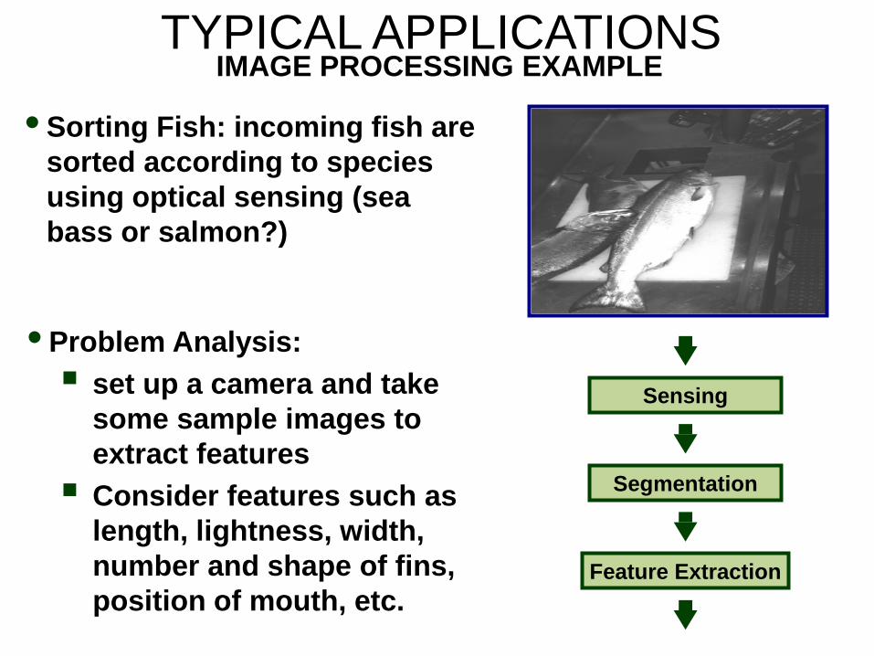
TYPICAL APPLICATIONS IMAGE PROCESSING EXAMPLE

• Sorting Fish: incoming fish are sorted according to species using optical sensing (sea bass or salmon?)

Feature Extraction

Segmentation

Sensing

• Problem Analysis: set up a camera and take

some sample images to extract features Consider features such as

length, lightness, width, number and shape of fins, position of mouth, etc.

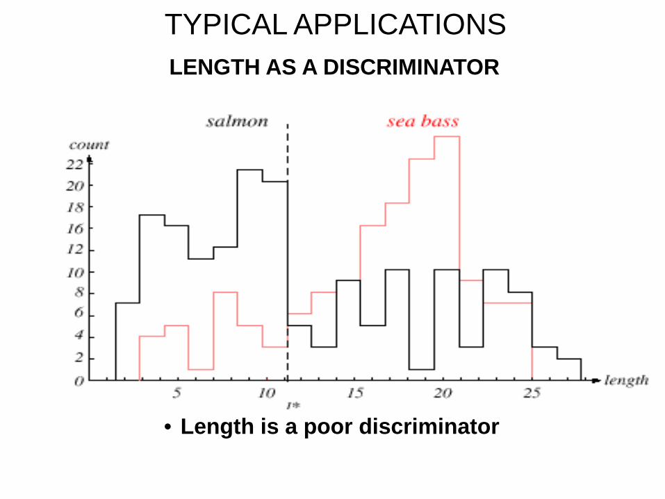
TYPICAL APPLICATIONS LENGTH AS A DISCRIMINATOR

• Length is a poor discriminator

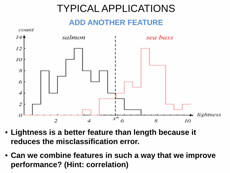
TYPICAL APPLICATIONS ADD ANOTHER FEATURE

• Lightness is a better feature than length because it reduces the misclassification error.

• Can we combine features in such a way that we improve performance? (Hint: correlation)

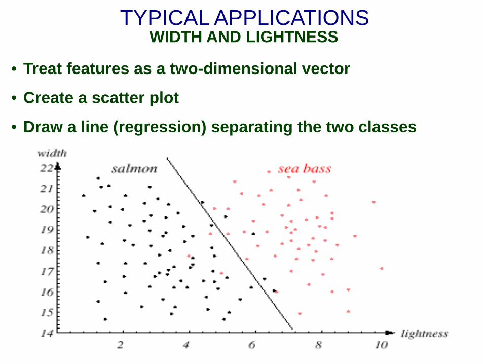
TYPICAL APPLICATIONS WIDTH AND LIGHTNESS

• Treat features as a two-dimensional vector

• Create a scatter plot

• Draw a line (regression) separating the two classes

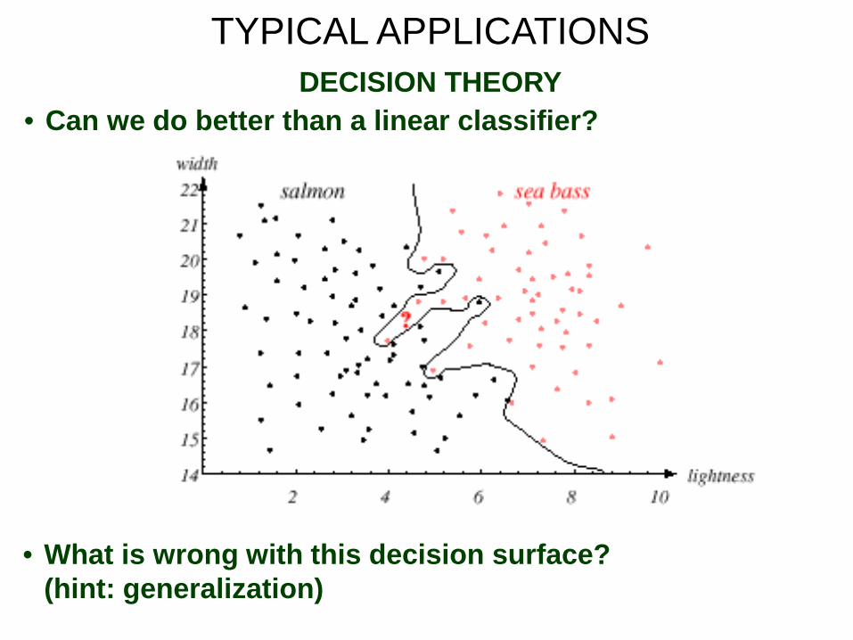
TYPICAL APPLICATIONS DECISION THEORY

• Can we do better than a linear classifier?

• What is wrong with this decision surface? (hint: generalization)

TYPICAL APPLICATIONS GENERALIZATION AND RISK

• Why might a smoother decision surface be a better choice?

• This course investigates how to find such “optimal” decision surfaces and how to provide system designers with the tools to make intelligent trade-offs.

Thomas Bayes

• At the time of his death, Rev. Thomas Bayes (1702 –1761) left behind two unpublished essays attempting to determine the probabilities of causes from observed effects. Forwarded to the British Royal Society, the essays had little impact and were soon forgotten.

• When several years later, the French

mathematician Laplace independently rediscovered a very similar concept, the English scientists quickly reclaimed the ownership of what is now known as the “Bayes Theorem”.

Bayesian decision theory is a fundamental statistical approach to the problem of pattern classification.

Quantify the tradeoffs between various classification decisions using probability and the costs that accompany these decisions.

Assume all relevant probability distributions are known (later we will learn how to estimate these from data).

Can we exploit prior knowledge in our fish classification problem: Are the sequence of fish predictable? (statistics) Is each class equally probable? (uniform priors) What is the cost of an error? (risk, optimization)

BAYESIAN DECISION THEORY PROBABILISTIC DECISION THEORY

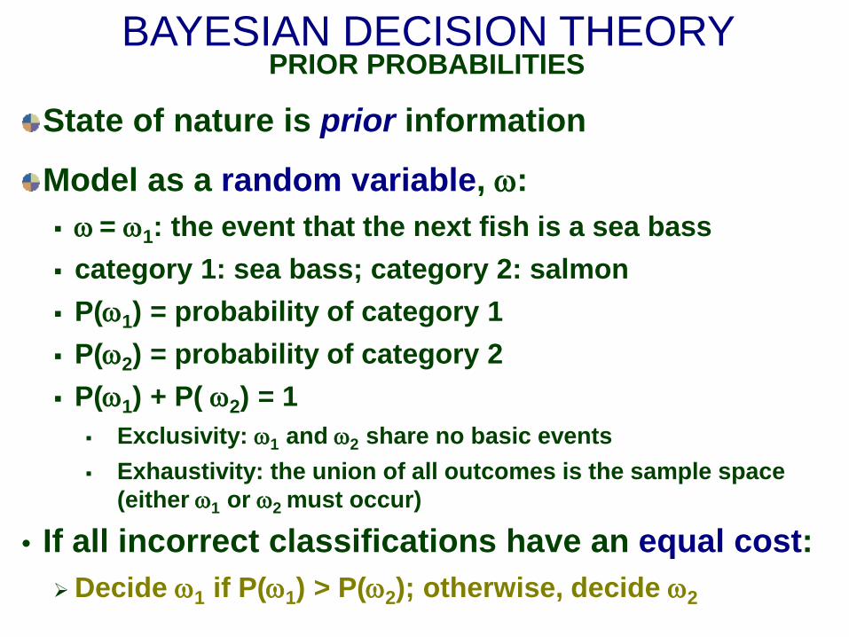
State of nature is prior information

Model as a random variable, ω: ω = ω1: the event that the next fish is a sea bass category 1: sea bass; category 2: salmon P(ω1) = probability of category 1 P(ω2) = probability of category 2 P(ω1) + P( ω2) = 1

Exclusivity: ω1 and ω2 share no basic events Exhaustivity: the union of all outcomes is the sample space

(either ω1 or ω2 must occur)

• If all incorrect classifications have an equal cost: Decide ω1 if P(ω1) > P(ω2); otherwise, decide ω2

BAYESIAN DECISION THEORY PRIOR PROBABILITIES

BAYESIAN DECISION THEORY CLASS-CONDITIONAL PROBABILITIES

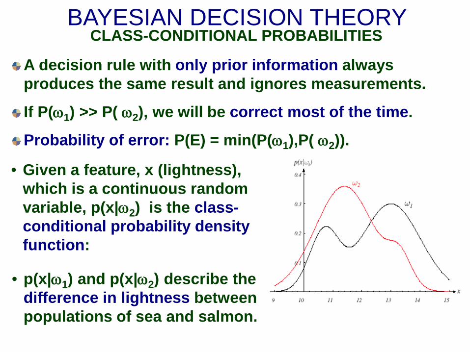
A decision rule with only prior information always produces the same result and ignores measurements.

If P(ω1) >> P( ω2), we will be correct most of the time.

Probability of error: P(E) = min(P(ω1),P( ω2)).

• Given a feature, x (lightness), which is a continuous random variable, p(x|ω2) is the class-conditional probability density function:

• p(x|ω1) and p(x|ω2) describe the difference in lightness between populations of sea and salmon.

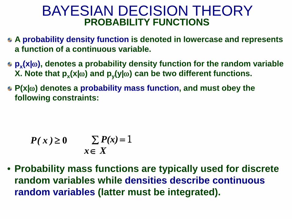
A probability density function is denoted in lowercase and represents a function of a continuous variable.

px(x|ω), denotes a probability density function for the random variable X. Note that px(x|ω) and py(y|ω) can be two different functions.

P(x|ω) denotes a probability mass function, and must obey the following constraints:

BAYESIAN DECISION THEORY PROBABILITY FUNCTIONS

1=∑∈ Xx

P(x)0≥)x(P

• Probability mass functions are typically used for discrete random variables while densities describe continuous random variables (latter must be integrated).

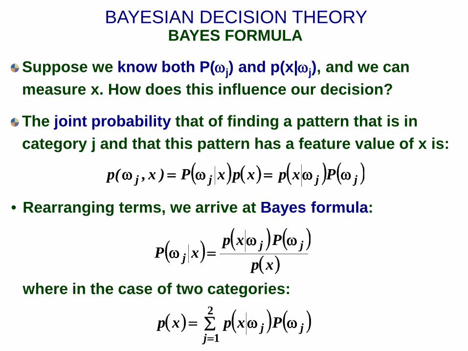
Suppose we know both P(ωj) and p(x|ωj), and we can measure x. How does this influence our decision?

The joint probability that of finding a pattern that is in category j and that this pattern has a feature value of x is:

( ) ( ) ( )( )xp

PxpxP jj

jωω

=ω

BAYESIAN DECISION THEORY BAYES FORMULA

( ) ( ) ( )jj

j Pxpxp ω∑ ω==

2

1

where in the case of two categories:

( ) ( ) ( ) ( )jjjj PxpxpxP)x,(p ωω=ω=ω

• Rearranging terms, we arrive at Bayes formula:

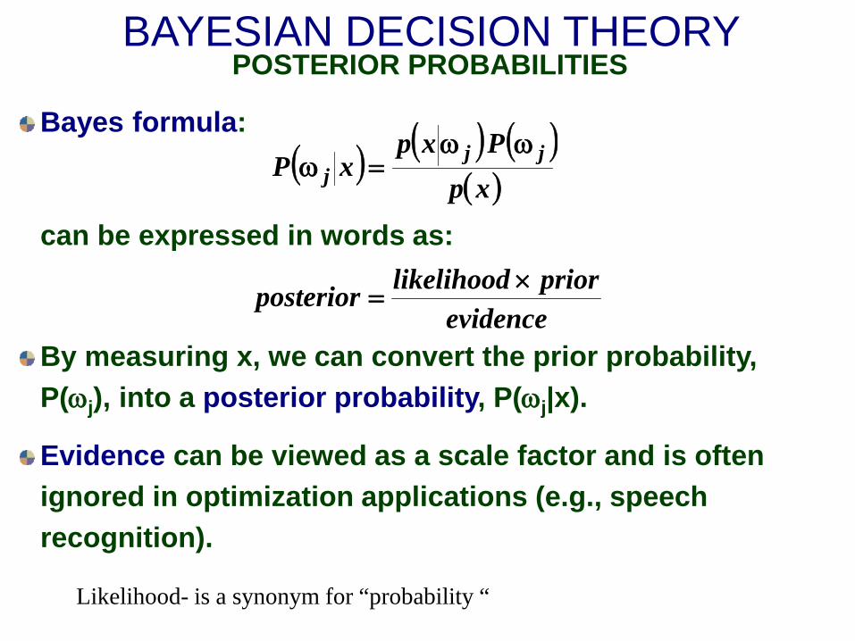
Bayes formula:

can be expressed in words as:

By measuring x, we can convert the prior probability, P(ωj), into a posterior probability, P(ωj|x).

Evidence can be viewed as a scale factor and is often ignored in optimization applications (e.g., speech recognition).

BAYESIAN DECISION THEORY POSTERIOR PROBABILITIES

( ) ( ) ( )( )xp

PxpxP jj

jωω

=ω

evidencepriorlikelihoodposterior ×

=

Likelihood- is a synonym for “probability “

BAYESIAN DECISION THEORY POSTERIOR PROBABILITIES

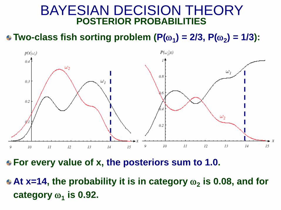
For every value of x, the posteriors sum to 1.0.

At x=14, the probability it is in category ω2 is 0.08, and for category ω1 is 0.92.

Two-class fish sorting problem (P(ω1) = 2/3, P(ω2) = 1/3):

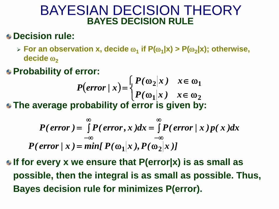
Decision rule: For an observation x, decide ω1 if P(ω1|x) > P(ω2|x); otherwise,

decide ω2

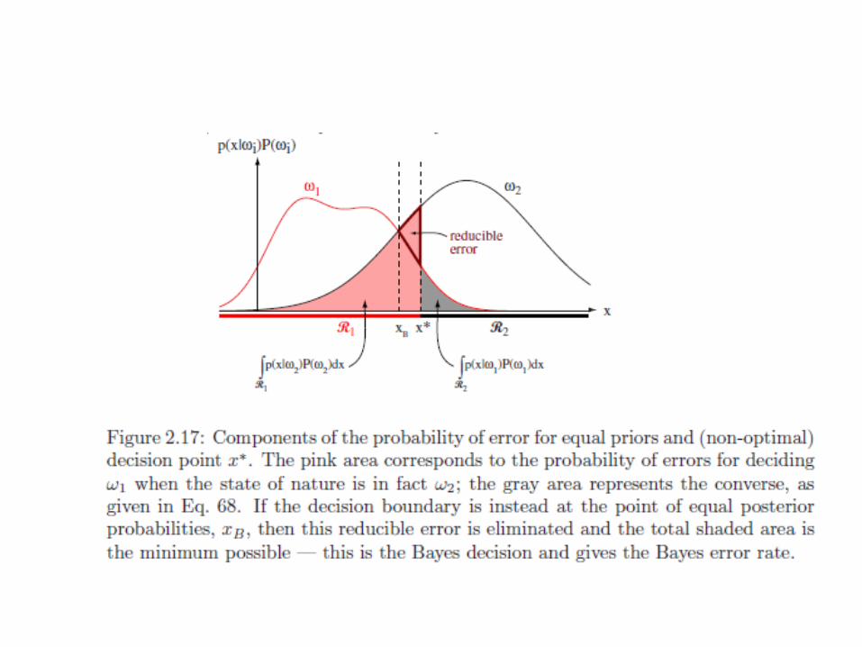
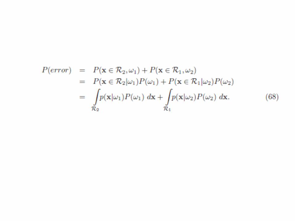
Probability of error:

The average probability of error is given by:

If for every x we ensure that P(error|x) is as small as possible, then the integral is as small as possible. Thus, Bayes decision rule for minimizes P(error).

BAYESIAN DECISION THEORY BAYES DECISION RULE

( )

ω∈ωω∈ω

=21

12

x)x(Px)x(P

x|errorP

∫∫ ==∞

∞−

∞

∞−dx)x(p)x|error(Pdx)x,error(P)error(P

)]x(P),x(Pmin[)x|error(P 21 ωω=

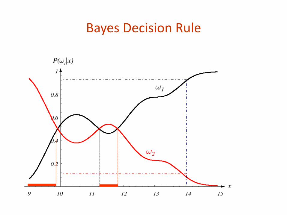
Bayes Decision Rule

BAYESIAN DECISION THEORY EVIDENCE

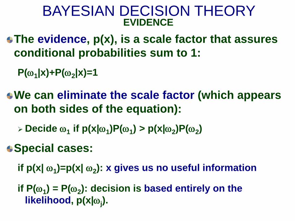
The evidence, p(x), is a scale factor that assures conditional probabilities sum to 1: P(ω1|x)+P(ω2|x)=1

We can eliminate the scale factor (which appears on both sides of the equation): Decide ω1 if p(x|ω1)P(ω1) > p(x|ω2)P(ω2)

Special cases: if p(x| ω1)=p(x| ω2): x gives us no useful information

if P(ω1) = P(ω2): decision is based entirely on the likelihood, p(x|ωj).

Generalization of the preceding ideas: Use of more than one feature

(e.g., length and lightness) Use more than two states of nature

(e.g., N-way classification) Allowing actions other than a decision to decide on the

state of nature (e.g., rejection: refusing to take an action when alternatives are close or confidence is low)

Introduce a loss of function which is more general than the probability of error (e.g., errors are not equally costly)

Let us replace the scalar x by the vector x in a d-dimensional Euclidean space, Rd, called the feature space.

CONTINUOUS FEATURES GENERALIZATION OF TWO-CLASS PROBLEM

CONTINUOUS FEATURES LOSS FUNCTION

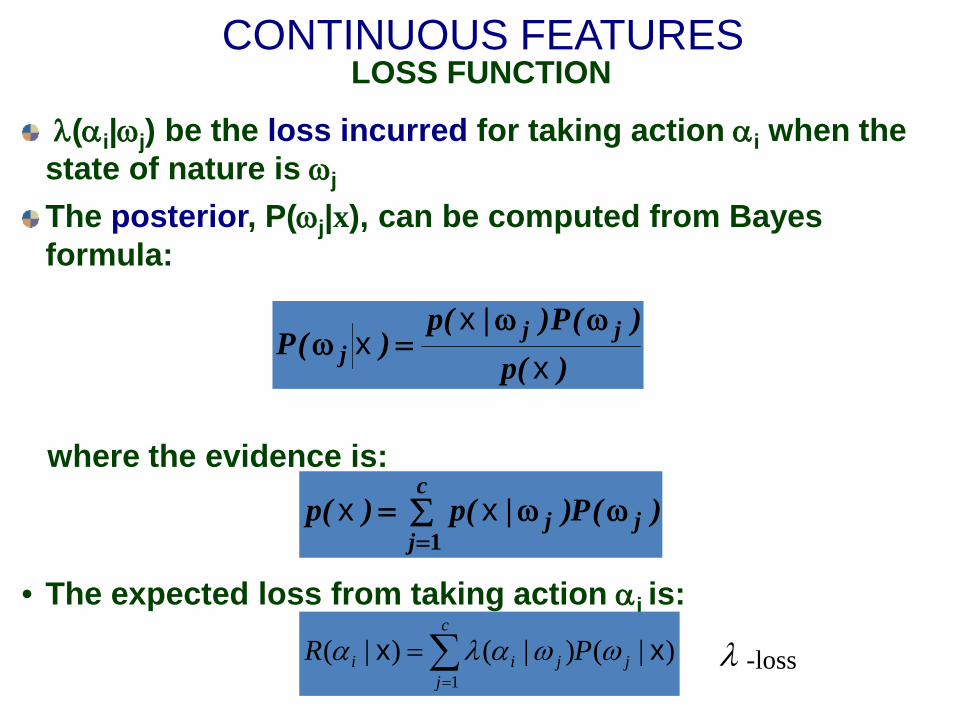
λ(αi|ωj) be the loss incurred for taking action αi when the state of nature is ωj

The posterior, P(ωj|x), can be computed from Bayes formula:

)(p)(P)|(p

)(P jjj x

xx

ωω=ω

where the evidence is: )(P)|(p)(p j

c

jj ω∑ ω=

=1xx

• The expected loss from taking action αi is: )|()|()|(

1xx j

c

jjii PR ωωαλα ∑

=

= λ -loss

CONTINUOUS FEATURES BAYES RISK

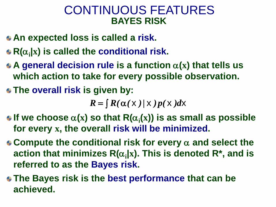
An expected loss is called a risk. R(αi|x) is called the conditional risk. A general decision rule is a function α(x) that tells us which action to take for every possible observation. The overall risk is given by:

∫ α= xxxx d)(p)|)((RRIf we choose α(x) so that R(αi(x)) is as small as possible for every x, the overall risk will be minimized. Compute the conditional risk for every α and select the action that minimizes R(αi|x). This is denoted R*, and is referred to as the Bayes risk. The Bayes risk is the best performance that can be achieved.

CONTINUOUS FEATURES TWO-CATEGORY CLASSIFICATION

Let α1 correspond to ω1, α2 to ω2, and λij = λ(αi|ωj) The conditional risk is given by:

R(α1|x) = λ11P(ω1|x) + λ12P(ω2|x) R(α2|x) = λ21P(ω1|x) + λ22P(ω2|x)

Our decision rule is: choose ω1 if: R(α1|x) < R(α2|x);

otherwise decide ω2 This results in the equivalent rule:

choose ω1 if: (λ21- λ11) P(ω1|x) > (λ12- λ22) P(ω2|x); otherwise decide ω2

If the loss incurred for making an error is greater than that incurred for being correct, the factors (λ21- λ11) and (λ12- λ22) are positive, and the ratio of these factors simply scales the posteriors.

CONTINUOUS FEATURES LIKELIHOOD

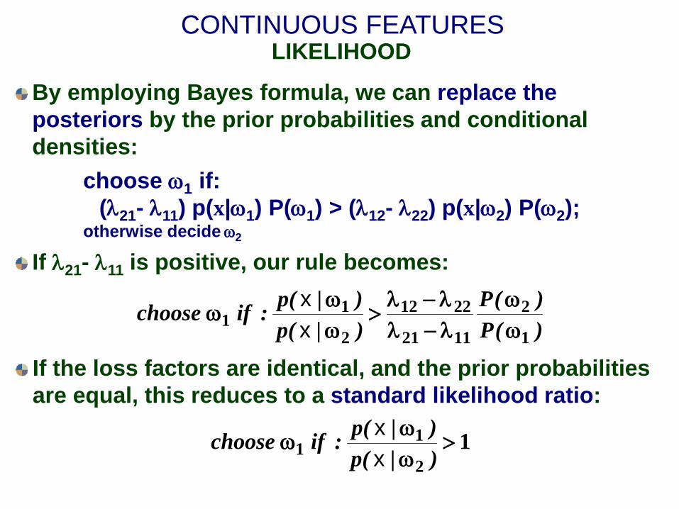
By employing Bayes formula, we can replace the posteriors by the prior probabilities and conditional densities:

choose ω1 if: (λ21- λ11) p(x|ω1) P(ω1) > (λ12- λ22) p(x|ω2) P(ω2);

otherwise decide ω2

If λ21- λ11 is positive, our rule becomes:

)(P)(P

)|(p)|(p:ifchoose

1

2

1121

2212

2

11 ω

ωλ−λλ−λ

>ωω

ωxx

If the loss factors are identical, and the prior probabilities are equal, this reduces to a standard likelihood ratio:

12

11 >

ωω

ω)|(p)|(p:ifchoose

xx

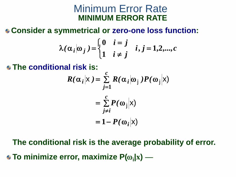
Consider a symmetrical or zero-one loss function:

Minimum Error Rate

=≠=

=ωαλ c,...,,j,ijiji

)( ji 2110

MINIMUM ERROR RATE

The conditional risk is:

x)

x)

x)x

j

jj

i

c

ij

c

jii

(P

(P

(P)(R)(R

ω−=

ω∑=

ω∑ ωα=α

≠

=

1

1

The conditional risk is the average probability of error.

To minimize error, maximize P(ωi|x) —

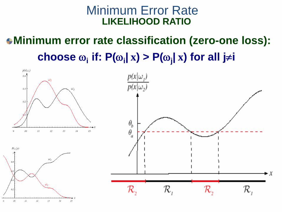
Minimum Error Rate LIKELIHOOD RATIO

Minimum error rate classification (zero-one loss): choose ωi if: P(ωi| x) > P(ωj| x) for all j≠i

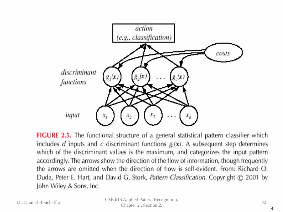
Classifiers, Discriminant Functions and Decision Surfaces

• The multi-category case – Set of discriminant functions gi(x), i = 1,…, c

– The classifier assigns a feature vector x to class ωi if gi(x) > gj(x) for all j ≠ i

Dr. Djamel Bouchaffra CSE 616 Applied Pattern Recognition, Chapter 2 , Section 2. 32

4


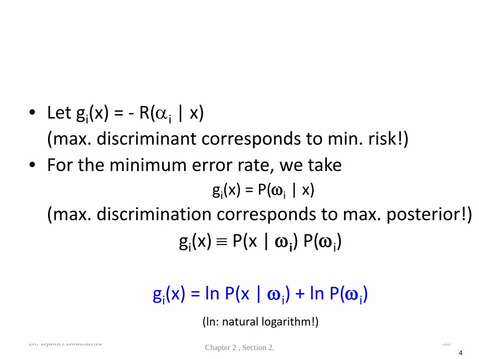
• Let gi(x) = - R(αi | x) (max. discriminant corresponds to min. risk!) • For the minimum error rate, we take

gi(x) = P(ωi | x) (max. discrimination corresponds to max. posterior!)

gi(x) ≡ P(x | ωi) P(ωi)

gi(x) = ln P(x | ωi) + ln P(ωi) (ln: natural logarithm!)

4


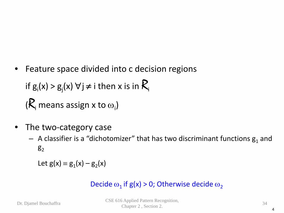
• Feature space divided into c decision regions

if gi(x) > gj(x) ∀j ≠ i then x is in Ri

(Ri means assign x to ωi)

• The two-category case – A classifier is a “dichotomizer” that has two discriminant functions g1 and

g2

Let g(x) ≡ g1(x) – g2(x)

Decide ω1 if g(x) > 0; Otherwise decide ω2

4


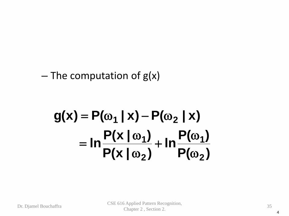
– The computation of g(x)

)(P)(Pln

)|x(P)|x(Pln

)x|(P)x|(P)x(g

2

1

2

1

21

ωω

+ωω

=

ω−ω=

4


4


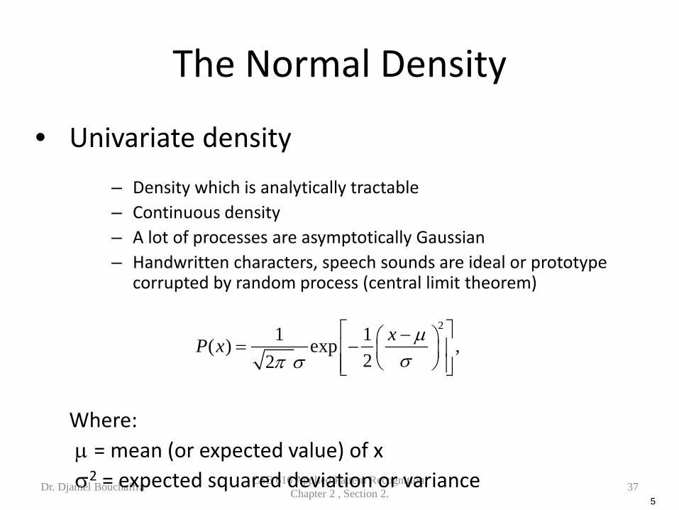
The Normal Density

• Univariate density

– Density which is analytically tractable – Continuous density – A lot of processes are asymptotically Gaussian – Handwritten characters, speech sounds are ideal or prototype

corrupted by random process (central limit theorem)

Where: µ = mean (or expected value) of x σ2 = expected squared deviation or variance

21 1( ) exp ,22

xP x µσπ σ

− = −

5


5

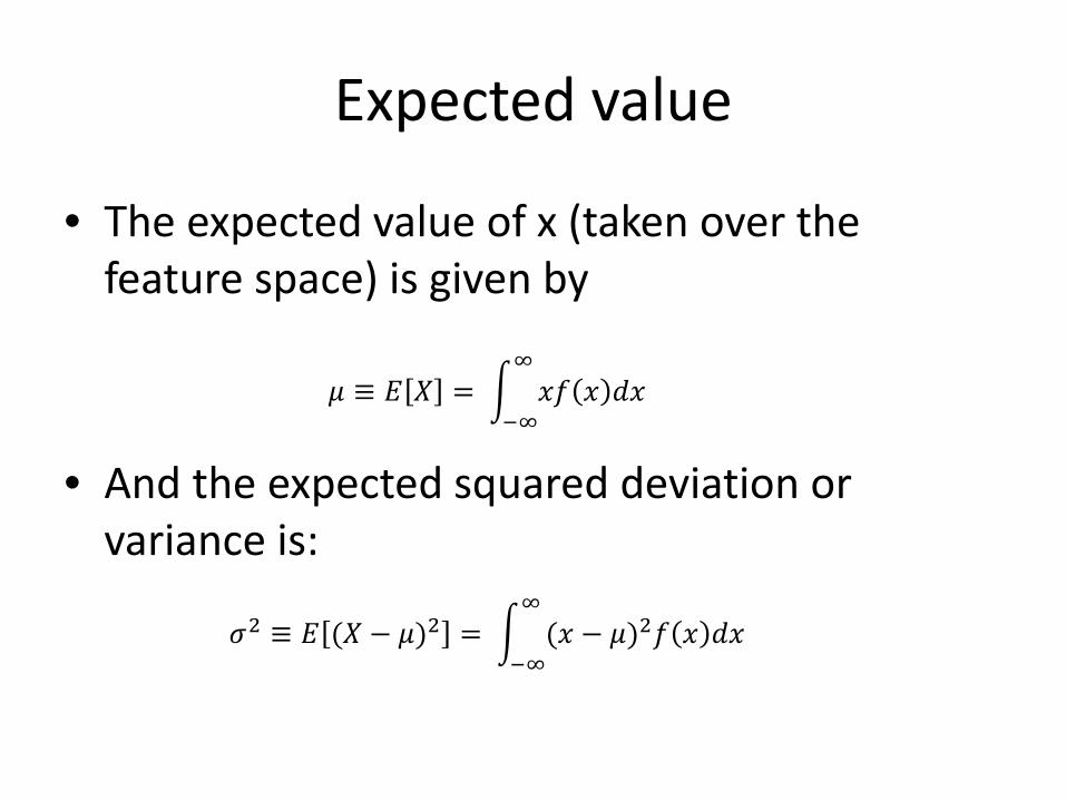
Expected value

• The expected value of x (taken over the feature space) is given by

• And the expected squared deviation or

variance is:

𝜇 ≡ 𝐸 𝑋 = � 𝑥𝑥 𝑥 𝑑𝑥∞

−∞

𝜎2 ≡ 𝐸 (𝑋 − 𝜇)2 = � (𝑥 − 𝜇)2𝑥 𝑥 𝑑𝑥∞

−∞


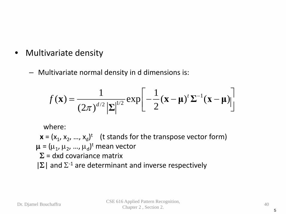
• Multivariate density – Multivariate normal density in d dimensions is:

where: x = (x1, x2, …, xd)t (t stands for the transpose vector form) µ = (µ1, µ2, …, µd)t mean vector Σ = dxd covariance matrix |Σ| and Σ-1 are determinant and inverse respectively

11/2/2

1 1( ) exp ( ) ( )2(2 )

td

fπ

− = − − − x x μ Σ x μ

Σ

5

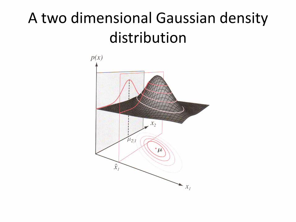
A two dimensional Gaussian density distribution

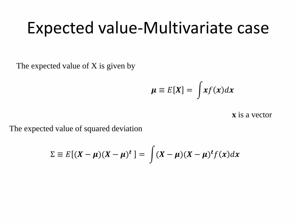
Expected value-Multivariate case

The expected value of X is given by

x is a vector

𝝁 ≡ 𝐸 𝑿 = �𝒙𝑥 𝒙 𝑑𝒙

The expected value of squared deviation

Σ ≡ 𝐸 (𝑿 − 𝝁)(𝑿 − 𝝁)𝒕 = �(𝑿 − 𝝁)(𝑿 − 𝝁)𝒕𝑥 𝒙 𝑑𝒙

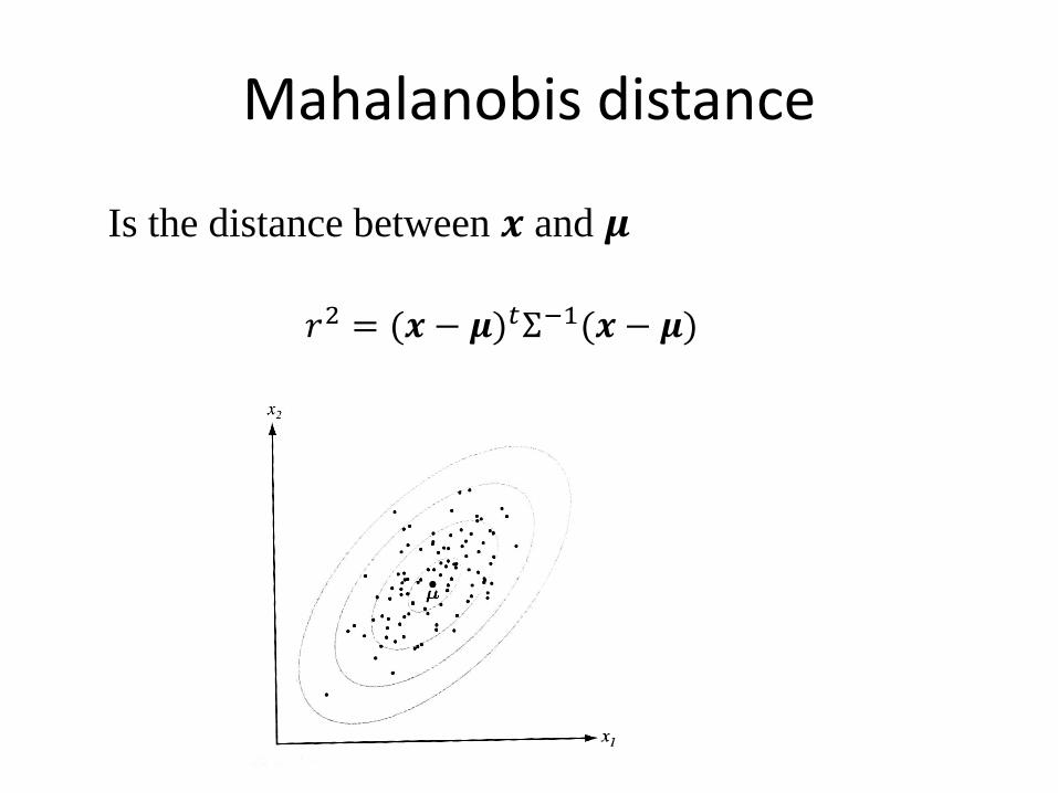
Mahalanobis distance

Is the distance between 𝒙 and 𝝁

𝑟2 = (𝒙 − 𝝁)𝑡Σ−1(𝒙 − 𝝁)

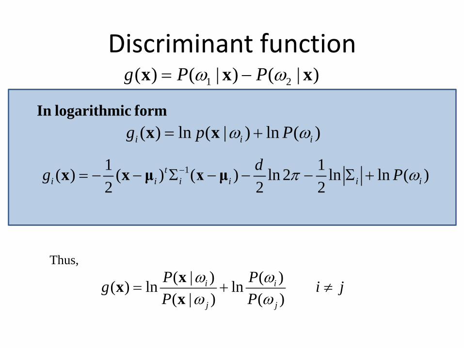
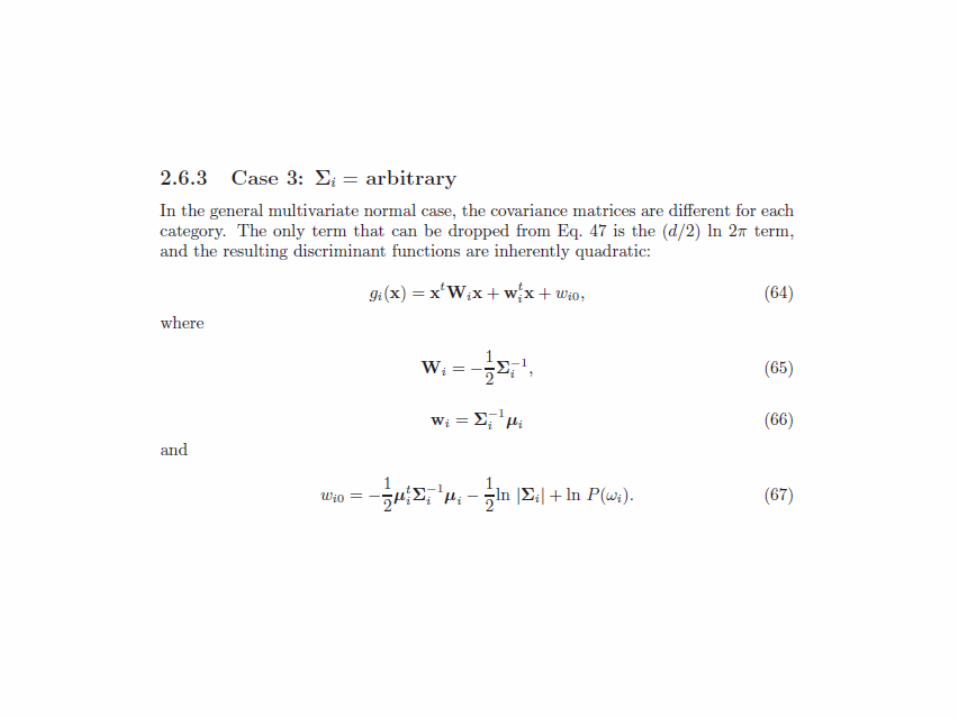
Discriminant function

( ) ln ( | ) ln ( )i i ig p Pω ω= +x x

11 1( ) ( ) ( ) ln 2 ln ln ( )2 2 2

ti i i i i i

dg Pπ ω−= − − Σ − − − Σ +x x μ x μ

1 2( ) ( | ) ( | )g P Pω ω= −x x x

In logarithmic form

Thus, ( | ) ( )( ) ln ln

( | ) ( )i i

j j

P Pg i jP P

ω ωω ω

= + ≠xxx

Case 1: Σi = σ2I Features are statistically independent, and all features have the

same variance: Distributions are spherical in d dimensions.

di

2

2

2

2

...00.........00...0000

σ

σ

σσ

=

=∑

6

Ii )/1( 21 σ=∑ −

i oft independen is2Ii σ=∑

GAUSSIAN CLASSIFIERS

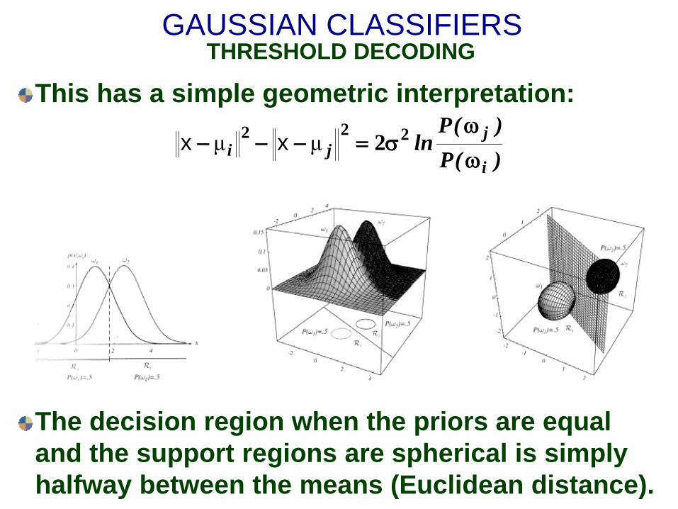
GAUSSIAN CLASSIFIERS THRESHOLD DECODING

This has a simple geometric interpretation:

)(P)(P

lni

jji ω

ωσ=−−− 222 2μμ xx

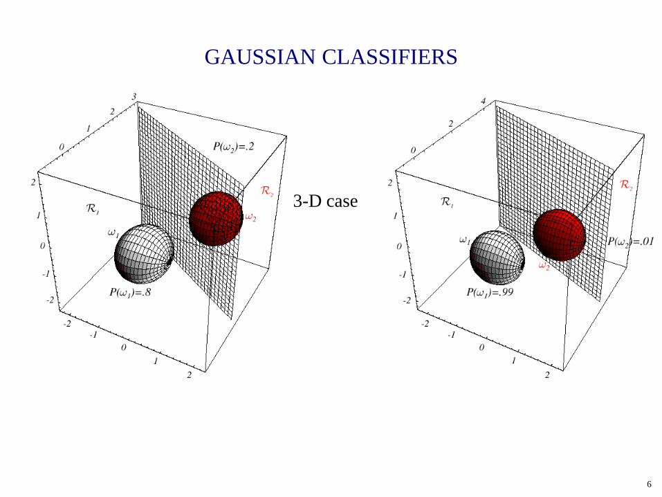
The decision region when the priors are equal and the support regions are spherical is simply halfway between the means (Euclidean distance).

6

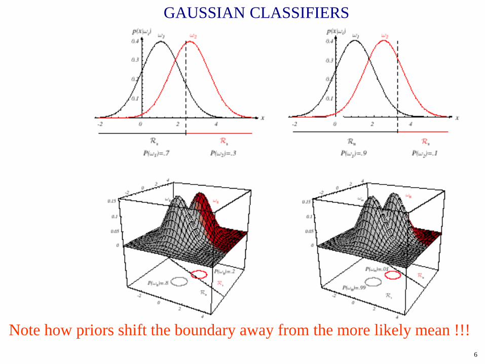
Note how priors shift the boundary away from the more likely mean !!!


6

3-D case


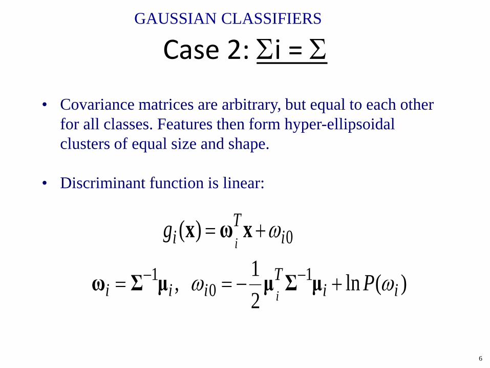
Case 2: Σi = Σ

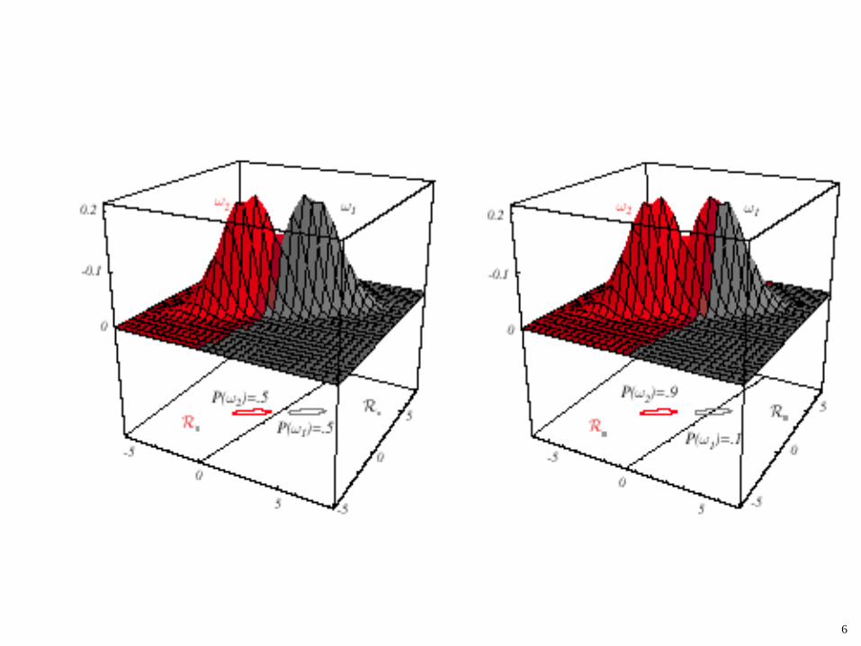
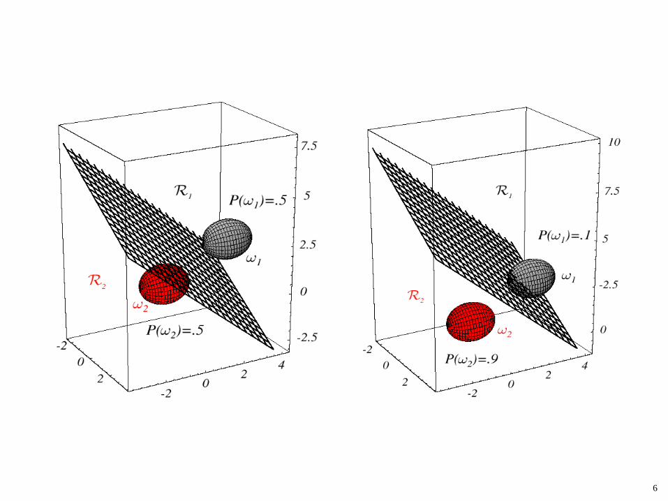
• Covariance matrices are arbitrary, but equal to each other for all classes. Features then form hyper-ellipsoidal clusters of equal size and shape.

• Discriminant function is linear:

6

0)( iT

i ig ω+= xωx

)(ln21 , 1

01

iiT

iii Pi

ωω +−== −− μΣμμΣω


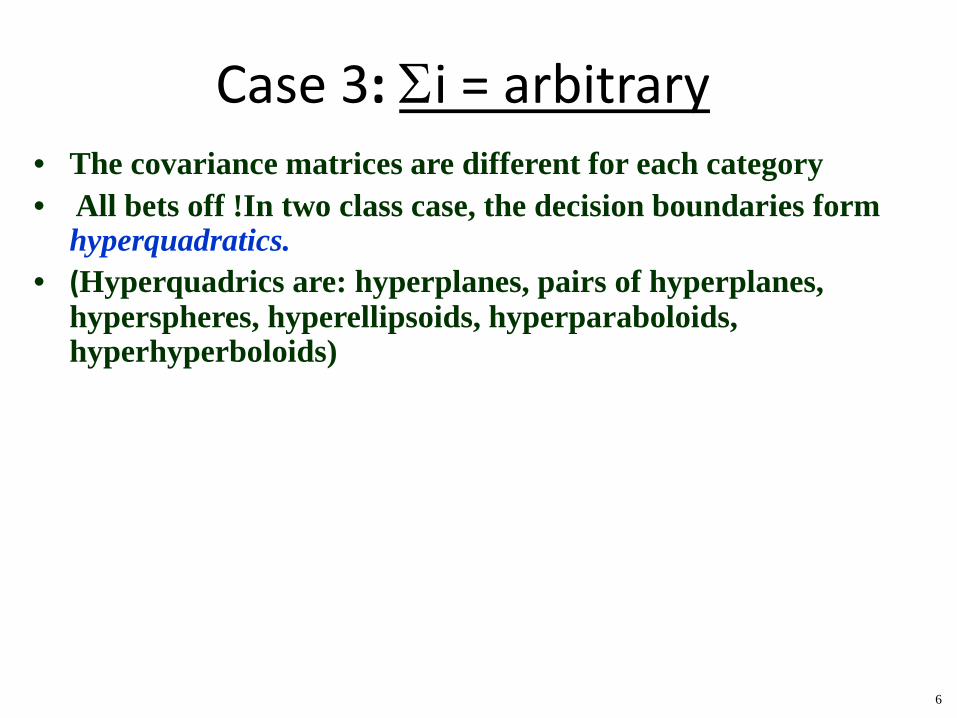
Case 3: Σi = arbitrary • The covariance matrices are different for each category • All bets off !In two class case, the decision boundaries form

hyperquadratics. • (Hyperquadrics are: hyperplanes, pairs of hyperplanes,

hyperspheres, hyperellipsoids, hyperparaboloids, hyperhyperboloids)

6

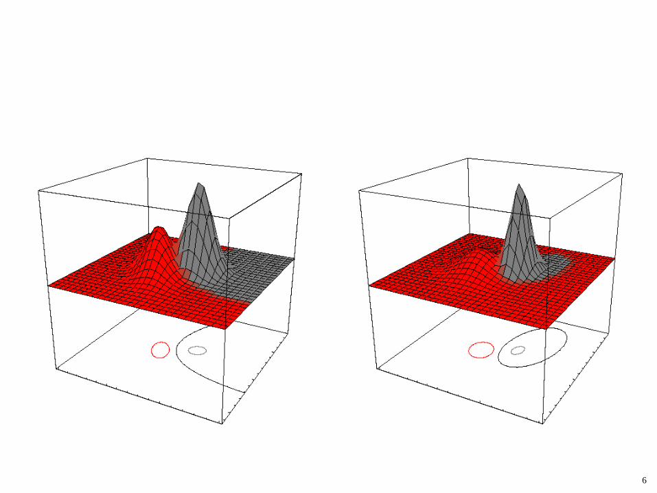
GAUSSIAN CLASSIFIERS ARBITRARY COVARIANCES

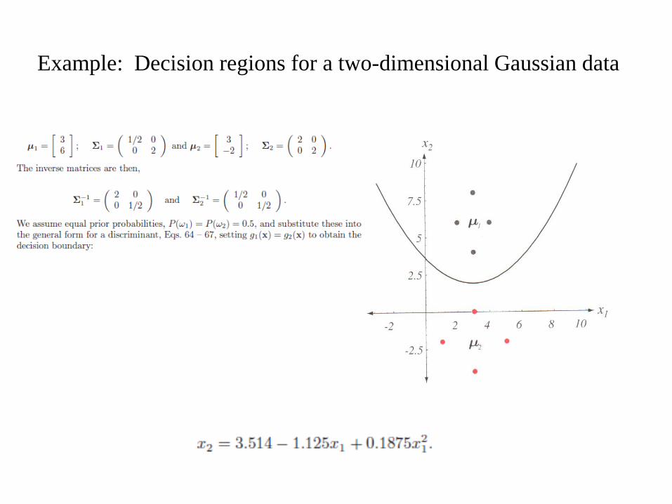
Example: Decision regions for a two-dimensional Gaussian data

Chi-Square Goodness-of-fit test

A special type of hypothesis test that is often used to test the equivalence of a probability density function of sampled data to some theoretical

density function is called the chi-squared goodness-of-fit test.

The procedure involves:

1. To use a statistics with an approximate chi-square distribution

2. To determine the degree of discrepancy between the observed and theoretical

3. To test an hypothesis of equivalence

Procedure

Consider a sample of N independent observations from a random variable x with a probability density p(x). Let N observations be grouped into K intervals, called class intervals, which together form a frequency histogram. The number of observations falling within the ith class interval is called the observed frequency fi. The theoretical numbers if the true pdf is po(x) is called the expected frequency, Fi

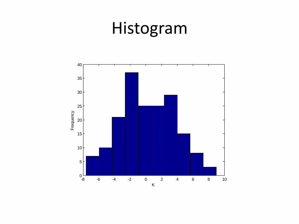
Histogram

-8 -6 -4 -2 0 2 4 6 8 100

5

10

15

20

25

30

35

40

K

Freq

uenc

y

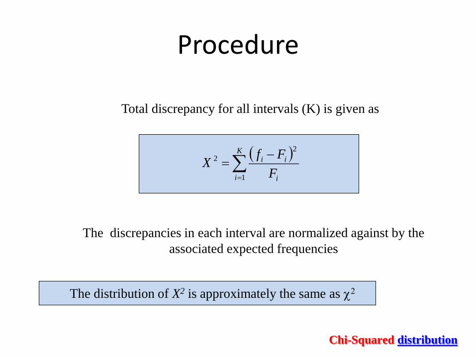
Procedure

Total discrepancy for all intervals (K) is given as

( )∑=

−=

K

i i

ii

FFfX

1

22

The discrepancies in each interval are normalized against by the associated expected frequencies

The distribution of X2 is approximately the same as χ2

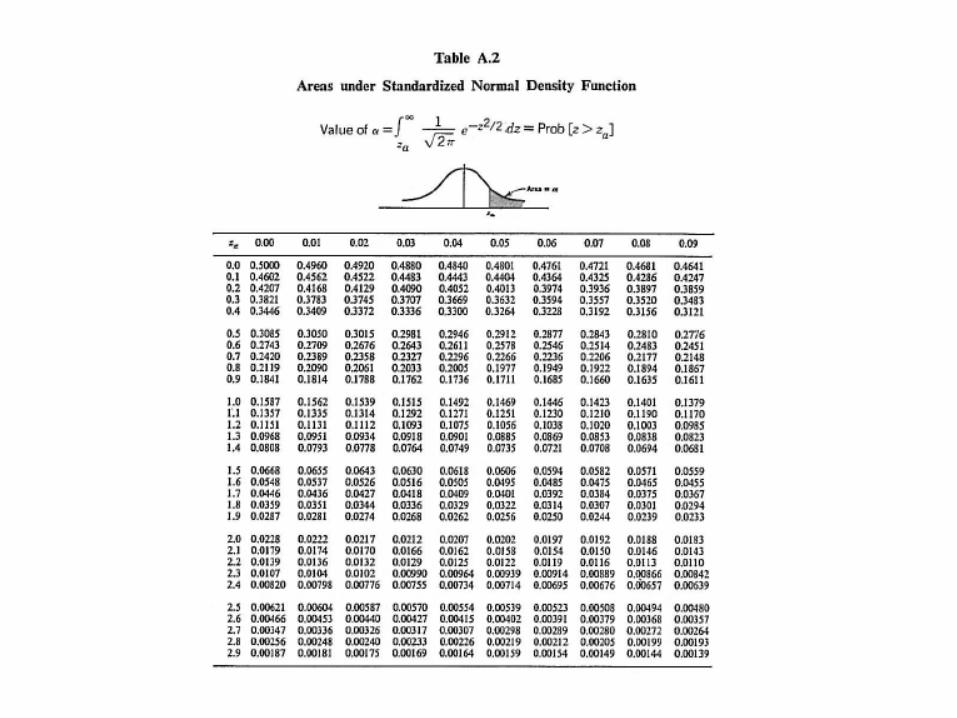
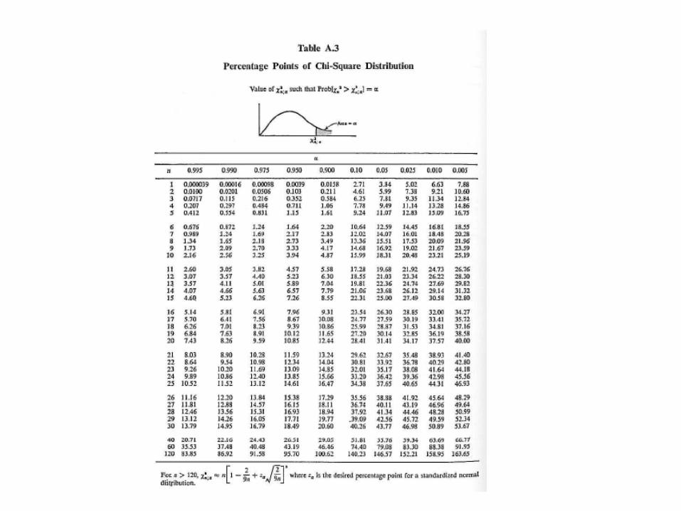
Chi-Squared distribution

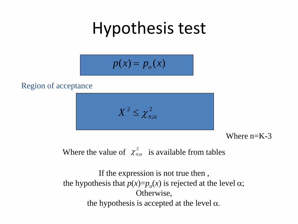
Hypothesis test

2;

2αχnX ≤

Where the value of is available from tables 2;αχn

If the expression is not true then , the hypothesis that p(x)=po(x) is rejected at the level α;

Otherwise, the hypothesis is accepted at the level α.

Where n=K-3

Region of acceptance

)()( xpxp o=

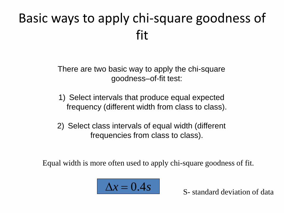
Basic ways to apply chi-square goodness of fit

There are two basic way to apply the chi-square goodness–of-fit test:

1) Select intervals that produce equal expected

frequency (different width from class to class).

2) Select class intervals of equal width (different frequencies from class to class).

Equal width is more often used to apply chi-square goodness of fit.

sx 4.0=∆ S- standard deviation of data

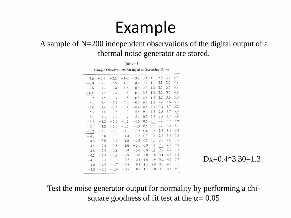
Example A sample of N=200 independent observations of the digital output of a

thermal noise generator are stored.

Test the noise generator output for normality by performing a chi-square goodness of fit test at the α= 0.05

Dx=0.4*3.30=1.3

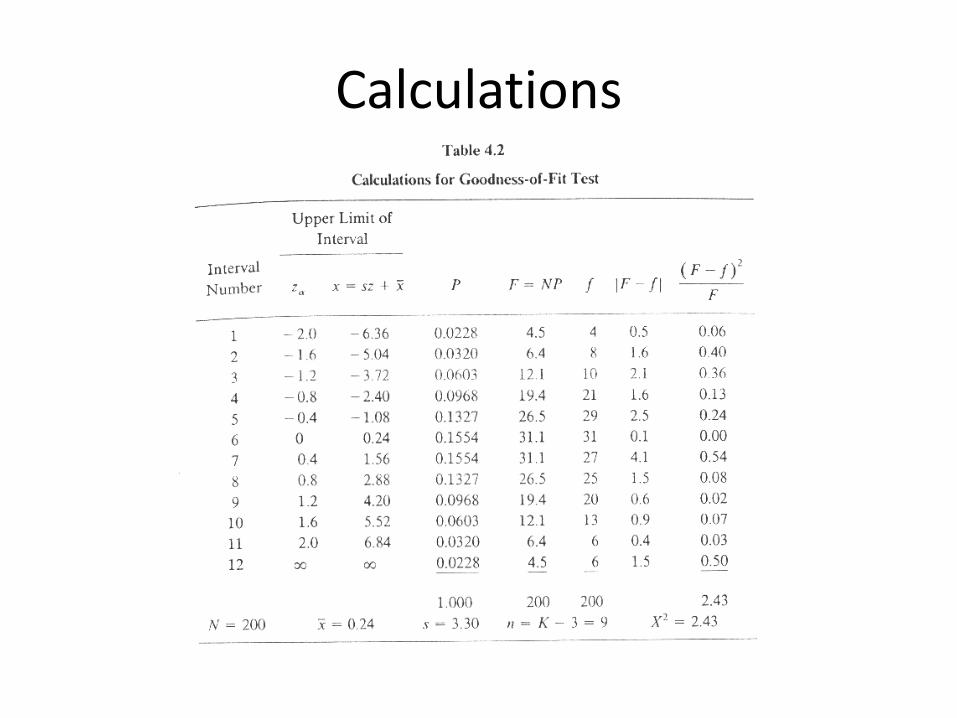
Calculations

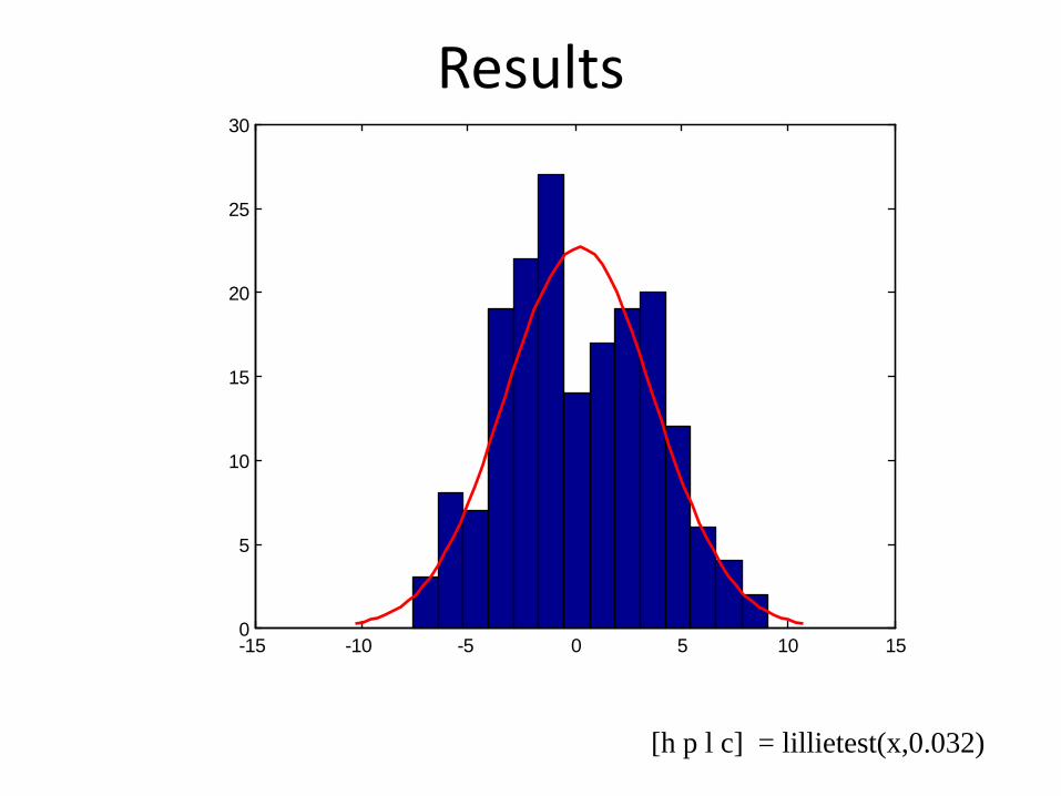
Results

-15 -10 -5 0 5 10 150

5

10

15

20

25

30

[h p l c] = lillietest(x,0.032)

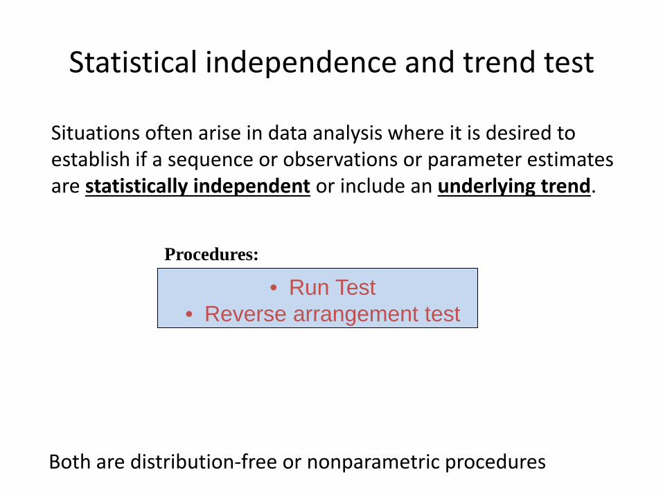
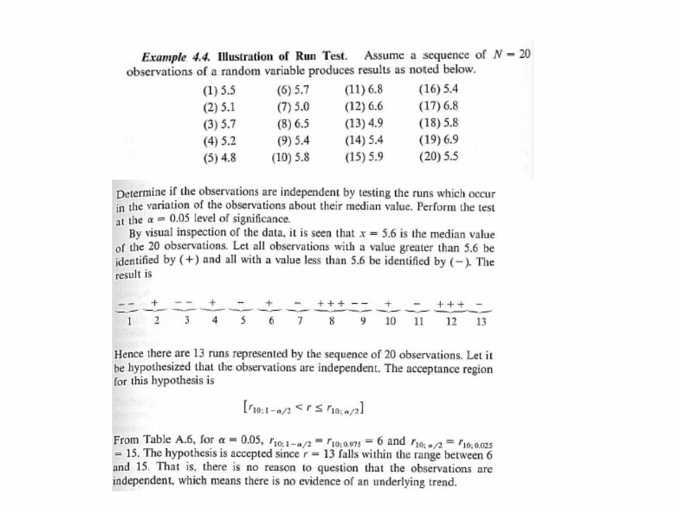
Statistical independence and trend test

Situations often arise in data analysis where it is desired to establish if a sequence or observations or parameter estimates are statistically independent or include an underlying trend.

• Run Test • Reverse arrangement test

Procedures:

Both are distribution-free or nonparametric procedures

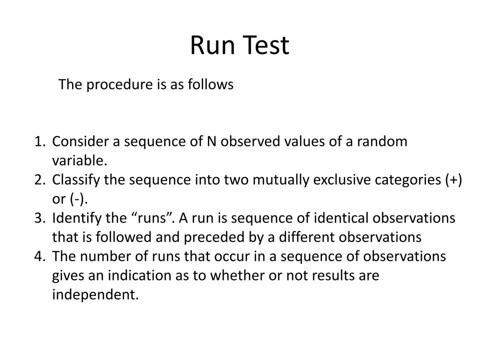
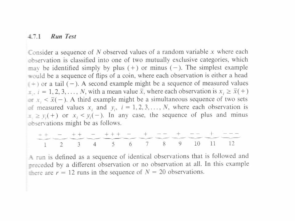
Run Test The procedure is as follows

1. Consider a sequence of N observed values of a random variable.

2. Classify the sequence into two mutually exclusive categories (+) or (-).

3. Identify the “runs”. A run is sequence of identical observations that is followed and preceded by a different observations

4. The number of runs that occur in a sequence of observations gives an indication as to whether or not results are independent.

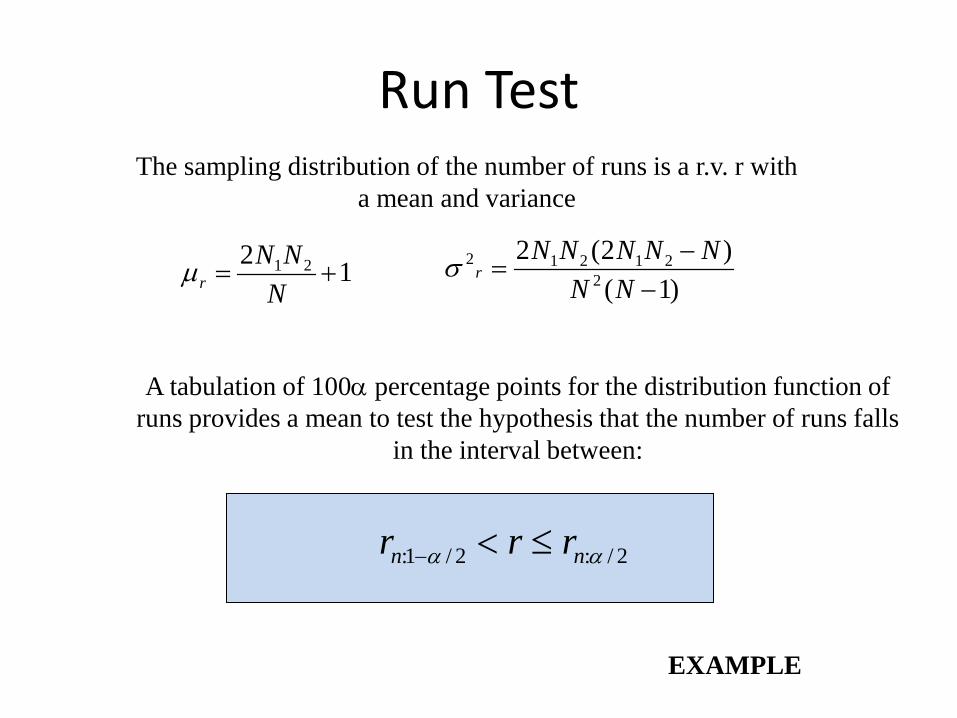
Run Test The sampling distribution of the number of runs is a r.v. r with

a mean and variance

12 21 +=N

NNrµ )1(

)2(22

21212

−−

=NN

NNNNNrσ

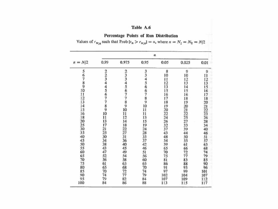
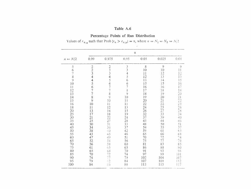
A tabulation of 100α percentage points for the distribution function of runs provides a mean to test the hypothesis that the number of runs falls

in the interval between:

2/:2/1: αα nn rrr ≤<−

EXAMPLE

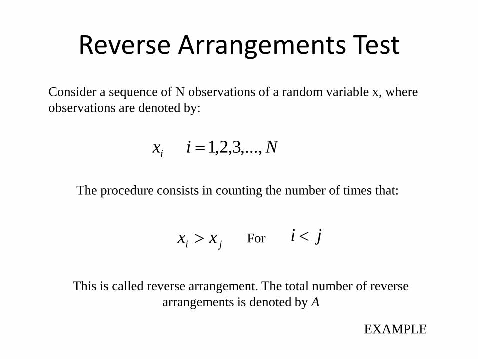
Reverse Arrangements Test Consider a sequence of N observations of a random variable x, where observations are denoted by:

Nixi ,...,3,2,1 =

The procedure consists in counting the number of times that:

ji xx > For ji <

This is called reverse arrangement. The total number of reverse arrangements is denoted by A

EXAMPLE

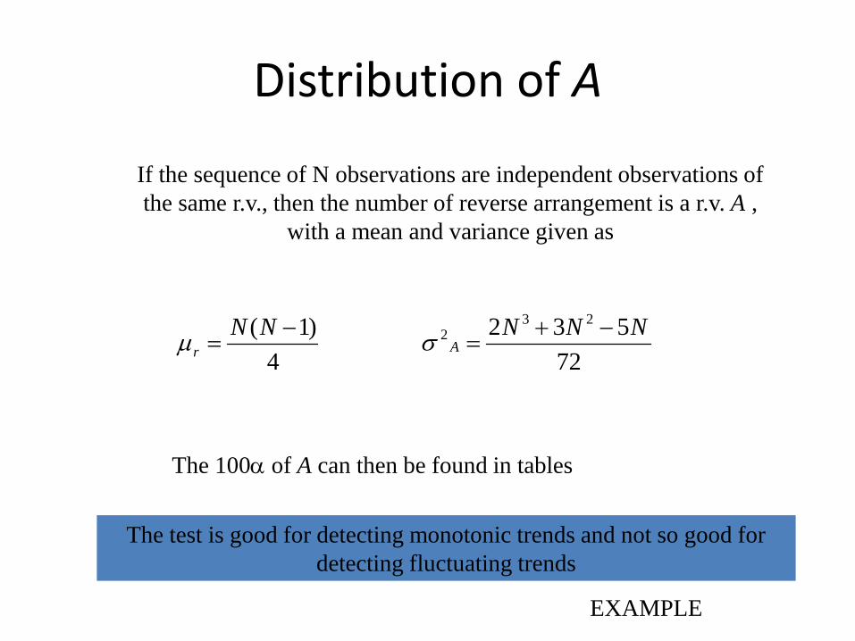
Distribution of A

If the sequence of N observations are independent observations of the same r.v., then the number of reverse arrangement is a r.v. A ,

with a mean and variance given as

4)1( −

=NN

rµ72

532 232 NNN

A−+

=σ

The 100α of A can then be found in tables

The test is good for detecting monotonic trends and not so good for detecting fluctuating trends

EXAMPLE

bayes&voice recognition

Documents