Bazaar: Enabling Predictable Performance in Datacenters

Virajith Jalaparti, Hitesh Ballani, Paolo Costa, Thomas Karagiannis, Antony RowstronMSR Cambridge, UK

Technical ReportMSR-TR-2012-38

Microsoft ResearchMicrosoft Corporation

One Microsoft WayRedmond, WA 98052

http://www.research.microsoft.com

1. INTRODUCTIONThe resource elasticity offered by cloud providers is of-

ten touted as a key driver for cloud adoption. Providersexpose a minimal interface– users or tenants simply askfor the compute instances they require and are chargedon a pay-as-you-go basis. Such resource elasticity en-ables elastic application performance; tenants can de-mand more or less compute instances to match perfor-mance needs.

While simple and elegant, there is a disconnect be-tween this low-level interface exposed by providers andwhat tenants actually require. Tenants are primarily in-terested in predictable performance and costs for theirapplications [1,2]; for instance, satisfying constraints re-garding their application completion time [3,4,5]. Withtoday’s setup, tenants bear the burden of translatingthese high-level goals into the corresponding resourcerequirements. Given the multiplicity of resources in adatacenter (compute instances, network, storage), sucha mapping requires determining how application perfor-mance scales with individual resources, which is oftennon-trivial.

The difficulty of mapping tenant goals is further exac-erbated by shared datacenter resources. While tenantsget dedicated compute instances with today’s cloud of-ferings, other resources like the internal network andthe cloud storage are shared and their performance canvary significantly [6,7,8]. This leads to unpredictableperformance for a wide-variety of applications, includ-ing user-facing online services [9,7], data analytics [7,10]and HPC applications [11]. Therefore, the task of de-termining the resources needed to achieve tenant goalswith today’s setup is intractable.

Apart from hurting cloud usability, the disconnect be-tween tenants and providers impedes cloud efficiencytoo. A lot of applications running in cloud datacen-ters are malleable in their resource requirements withmultiple resource combinations yielding the same per-formance. For instance, a completion time goal for aMapReduce job may be achieved through a few virtualmachines (VMs) with a lot of network bandwidth be-tween them, a lot of VMs with a little network band-width, or somewhere in between these extremes. Ten-ants making resource choices in isolation so as to satisfytheir goals can result in sub-optimal choices that reducesystem throughput.

Overall, the skewed division of functionality betweentenants and providers imposed by today’s setup hurtsboth entities; tenants cannot achieve predictable per-formance while providers lose revenue due to inefficientoperation.

The problem of unpredictable performance has promptedefforts to provide guaranteed performance atop shareddatacenter resources like the internal network [2,12,13]and cloud storage [14,15]. These proposals allow ten-

ants to explicitly request for resources beyond com-pute instances, thus enabling true multi-resource elas-ticity. While necessary, these techniques are not suffi-cient. Even with guaranteed resources, automaticallyinferring how the performance of an arbitrary applica-tion scales with various resources is hard. Expecting aprogrammer to explicitly understand and describe howthe program scales with each resource is also impracti-cal.

In this paper, we take a first stab at enabling pre-dictable application performance in cloud datacenters.Our examination of typical cloud applications from threedifferent domains (data analytics, web-facing, MPI) showsthat they exhibit both resource malleability and perfor-mance predictability, two key conditions that our tar-get applications must satisfy. For such applications, wedevise mechanisms to choose the resource combinationthat can achieve tenant performance goals and is mostsuitable for the provider. Thus, the impetus of this pa-per is on ensuring predictable performance while capi-talizing on resource malleability.

We illustrate these mechanisms in the context of dataanalytics by focusing on MapReduce as an examplecloud application. We designed Bazaar, a system thattakes tenant constraints regarding the completion time(or cost) for their MapReduce job and determines theresource combination most amenable to the providerthat satisfies the constraints. Our choice of MapReducewas motivated by the fact that data analytics representa significant workload for cloud infrastructures [16,17],with some multi-tenant datacenters having entire clus-ters dedicated to running them [18,19,20]. Further, themalleability and predictability conditions described abovehold very well for MapReduce.

Though our core ideas apply to general multi-resourcesettings, we begin by focusing on two specific resources,compute instances (N) and the network bandwidth (B)between them. Bazaar uses a performance predictioncomponent to determine the resource tuples < N,B >that can achieve the desired completion time. As mul-tiple resource tuples may achieve the same completiontime, they are ranked in terms of the provider’s costto accommodate the tuple. Bazaar selects the resourcetuple with the least provider cost, thus improving pro-vider efficiency. Overall, this paper makes the followingcontributions:

• We measure the malleability of representative cloudapplications, and show that different combinations ofcompute and network resources can achieve the sameapplication performance.

• We present a gray-box approach to predict how theperformance of a MapReduce job scales in terms ofmultiple resources. The prediction is fast, low over-head and has good accuracy (<12% average error).

1

• We devise a metric for the cost of multi-resource re-quests from the provider’s perspective. This allowsone resource tuple to be compared against another.

• We present the design and implementation of Bazaar,and use it to illustrate how tenants can achieve theirperformance goals in a multi-resource setting.

Using extensive large-scale simulations and deploy-ment on a small testbed, we show that smart resourceselection to satisfy tenant goals can yield significantgains for the provider. The provider can accept 3-14%more requests. Further, bigger (resource intensive) re-quests can be accepted which improves the datacentergoodput by 7-87%.

Since there are no well established pricing models formulti-resource requests like the ones considered here,this paper intentionally focuses on completion time goalsand datacenter goodput. Towards the end of the paper,we briefly discuss a novel pricing model that, when cou-pled with Bazaar, can allow tenants to achieve their costgoals too. We also discuss how exploiting malleabilityof more than two resources can be accomodated withBazaar, and, as an example, provide a case-study ex-ploiting malleability along the time domain. Our find-ings show that exploiting time malleability can furtherreduce median job completion time by more than 50%.Overall, we argue that the higher-level tenant-providerinterface enabled by Bazaar benefits both entities. Ten-ants achieve their goals, while the resource selectionflexibility improves datacenter goodput and hence, pro-vider revenue.

On a broader note, the resource elasticity enabled bycloud computing can allow tenants to trade-off highercosts for better performance. Bazaar makes this trade-off explicit for MapReduce-like applications. We believethat if such elasticity of performance and costs were tobe extended to a broader set of applications, it wouldremove a major hurdle to cloud adoption.

2. BACKGROUND AND MOTIVATIONCloud providers today allow tenants to ask for vir-

tual machines or VMs on demand. The VMs can varyin size– small, medium or large VMs are typically of-fered reflecting the available processing power, memoryand local storage. For ease of exposition, the discussionhere assumes a single VM class. A tenant request canbe characterized by N , the number of VMs requested.Tenants pay a fixed amount per hour per VM; thus,renting N VMs for T hours costs $kv ∗NT , where kv isthe hourly VM price. For Amazon EC2, kv = $0.08 forsmall VMs.

Data analytics in the cloud. Analysis of big datasets underlies many web businesses [21,16,17] migrat-ing to the cloud. Data-parallel frameworks like MapRe-duce [22], Dryad [23], or Scope [19] cater to such data

analytics, and form a key component of cloud work-loads. Despite a few differences, these frameworks arebroadly similar and operate as follows: Each job typi-cally consists of three phases, (i). reading input data andapplying a grouping function, (ii). shuffling intermediatedata among the compute nodes across the network, (iii).applying an aggregation function to generate the finaloutput. For example, in the case of MapReduce, thesephases are known as map, shuffle, and reduce phases.Computation may involve a series of such jobs.

Predictable performance. The parallelism providedby data parallel frameworks is an ideal match for theresource elasticity offered by cloud computing since thecompletion time of a job can be tuned by varying the re-sources devoted to it. Tenants often have high-level per-formance or cost requirements for their data-analytics.Such requirements may dictate, for example, that a jobneeds to finish in a timely fashion. However, with to-day’s setup, tenants are responsible for mapping suchhigh-level completion time goals down to specific re-sources needed for their jobs [3,4]. This has led to aslew of proposals for optimization, mostly focusing onMapReduce– determining good configuration parame-ters [4], storage and compute resources [3], and betterscheduling [24]. Recent efforts like Elasticiser [5] addressthe problem at a higher-level and strive to determine thenumber and type of VMs needed to ensure a MapRe-duce job achieves the desired completion time.

Yet, the performance of most data analytic jobs de-pends on factors well-beyond the number of VMs de-voted to them. For instance, apart from the actual pro-cessing of data, a job running in the cloud also in-volves reading input data off the cloud storage serviceand shuffling data between VMs over the internal net-work. Since the storage service and the internal networkare shared resources, their performance can vary signif-icantly [6,7,8]. This, in turn, impacts application per-formance, irrespective of the number of assigned VMs.For instance, Schad et al. [7] found that the completiontime of the same job executing on the same numberof VMs on Amazon EC2 can vary considerably, withthe underlying network contributing significantly to thevariation. Thus, without accounting for resources beyondsimply the compute units, the goal of determining thenumber of VMs needed to achieve a desired completiontime is practically infeasible. We show evidence of thisin § 4.2.2.

At the same time, ignoring the tenant’s requirementshurts providers as well. For instance, it results in poorVM placement and high contention across the internaldatacenter network. This leads to poor performing jobsthat prevent the provider from accepting subsequenttenant requests. Such outliers have been shown to dragdown the system throughput and, hence, the providerrevenue by as much as 60% [2].

2

Multi-resource elasticity. Performance issues withshared resources, such as the ones described above, haveprompted a slew of proposals that offer guaranteed per-formance atop such resources [2,12,13,14,15]. With these,tenants can request resources beyond just VMs; for in-stance, [2,12,13] allow tenants to specify the networkbandwidth between their VMs. We note that provid-ing tenants with a guaranteed amount of individual re-sources makes the problem of achieving high-level per-formance goals tractable.

This paper exploits such multi-resource elasticity andbuilds upon efforts that provide guaranteed resources.We consider a two resource tenant-provider interfacewhereby tenants can ask for VMs and internal networkbandwidth. As proposed in [2,12], a tenant request ischaracterized by a two tuple <N,B> which gives thetenant N VMs, each with an aggregate network band-width of B Mbps to other VMs of the same tenant.However, before discussing how such resource elasticitycan be exploited, we first quantify its impact on typicalcloud applications.

2.1 Malleability of data-analytics applicationsWe first focus on data analytic frameworks, and use

MapReduce as a running example. Our goal is to studyhow its performance is affected when varying differentresources.

Hadoop Job Input Data Set

Sort 200GB using Hadoop’s RandomWriterWordCount 68GB of Wikipedia articlesGridmix 200GB using Hadoop’s RandomTextWriterTF-IDF 68GB of Wikipedia articles

LinkGraph 10GB of Wikipedia articles

Table 1: MapReduce jobs and the size of theirinput data

We experimented with the small yet representativeset of MapReduce jobs listed in Table 1. These jobscapture the use of data analytics in different domainsand the varying complexity of such workloads (throughmulti-stage jobs). Sort and WordCount are popular forMapReduce performance benchmarking, not to mentiontheir use in business data processing and text anal-ysis respectively [25]. Gridmix is a synthetic bench-mark modeling production workloads, Term Frequency-Inverse Document Frequency or TF-IDF is used in infor-mation retrieval, and LinkGraph is used to create largehyperlink graphs. Of these, Gridmix, LinkGraph, andTF-IDF are multi-stage jobs.

We used Hadoop MapReduce on Emulab to executethe jobs while varying the number of nodes devoted tothem (N). We also used rate-limiting on the nodes tocontrol the network bandwidth between them (B). Foreach <N,B> tuple, we executed a job fives times tomeasure the completion time for the job and its indi-vidual phases. While the experiment setup is further

0

100

200

300

400

500

600

50 100 150 200 250 300

Com

ple

tion T

ime (

sec)

Network Bandwidth (Mbps)

N=10N=20

(a) LinkGraph

0

2000

4000

6000

8000

50 100 150 200 250 300

Com

ple

tion T

ime (

sec)

Network Bandwidth (Mbps)

N=10N=20

(b) Sort

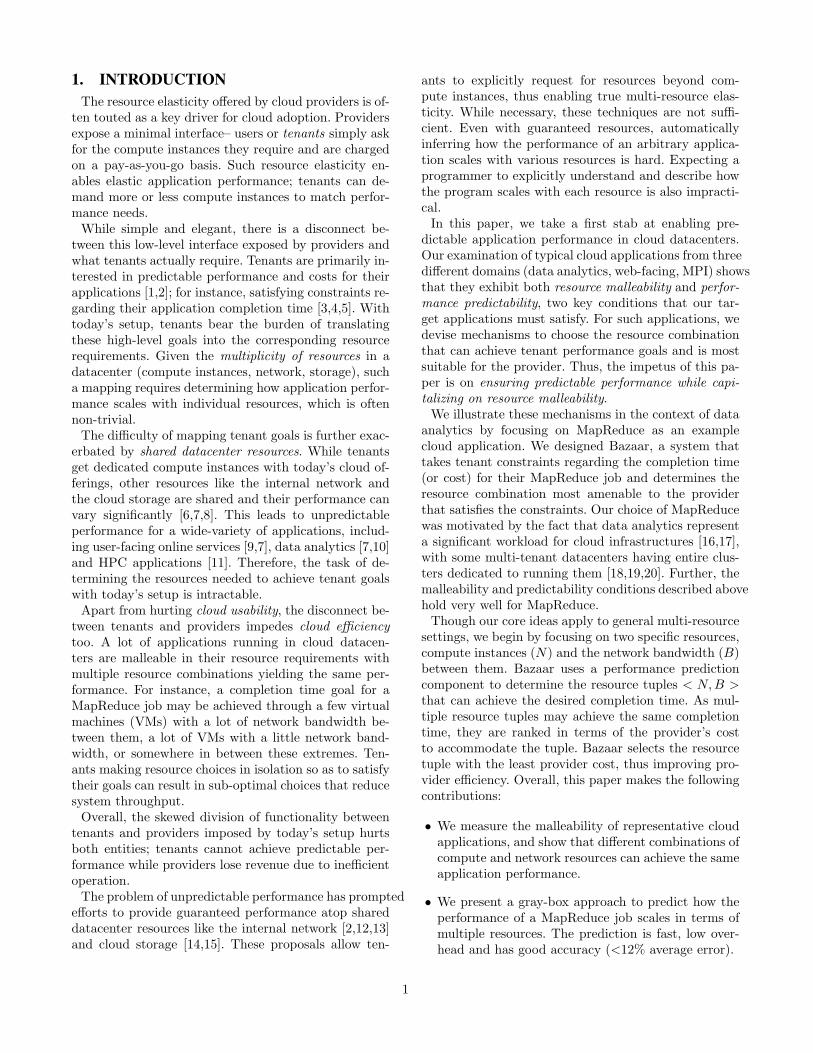
Figure 1: Completion time for jobs with varyingnetwork bandwidth. Error bars represent Min–Max values.

detailed in §4.1, here we just focus on the performancetrends.

Figure 1(a) shows the completion time for LinkGraphon a cluster with 10 and 20 nodes and varying net-work bandwidth. As the bandwidth between the nodesincreases, the time to shuffle the intermediate data be-tween map and reduce tasks shrinks, and thus, the com-pletion time reduces. However, the total completion timestagnates beyond 250 Mbps. This is because the localdisk on each node provides an aggregate bandwidth of250 Mbps. Hence, increasing the network bandwidth be-yond this value does not help since the job completiontime is dictated by the disk performance. This is an ar-tifact of the disks on the testbed nodes. If the disks wereto offer higher bandwidth, increasing the network band-width beyond this value would still shrink the comple-tion time. This was also confirmed by the experimentsthat we ran on our testbed (see Section 4.3) where weused in-memory data shuffle to avoid incurring the diskbottleneck.

The same trend holds for the other jobs we tested. Forinstance, Figure 1(b) shows that the completion timefor Sort reduces as the number of nodes and the net-work bandwidth between the nodes is increased. Notehowever that the precise impact of either resource is job-specific. For instance, we found that the relative dropin completion time with increasing network bandwidthis greater for Sort than for WordCount. This is becauseSort is I/O intensive with a lot of data shuffled whichmeans that its performance is heavily influenced by thenetwork bandwidth between the nodes.

Apart from varying network bandwidth, we also exe-cuted the jobs with varying number of nodes. While theresults are detailed in Section 4.1 (Figures 6(a) and 7(a)),we find that the completion time for a job is inverselyproportional to the number of nodes devoted to it. Thisis a direct consequence of the data-parallel nature ofMapReduce.

2.2 Malleability of other cloud applicationsThe findings in the previous section extend to other

3

0 50

100 150 200 250 300 350 400 450 500

100 1000

Thro

ughput

(req

s/se

c)

Network Bandwidth (Mbps)

N=4N=2N=1

(a) Web application

0

2000

4000

6000

8000

10000

10 100 1000

Com

ple

tion T

ime (

sec)

Network Bandwidth (Mbps)

N=8N=12N=16

(b) MPI application

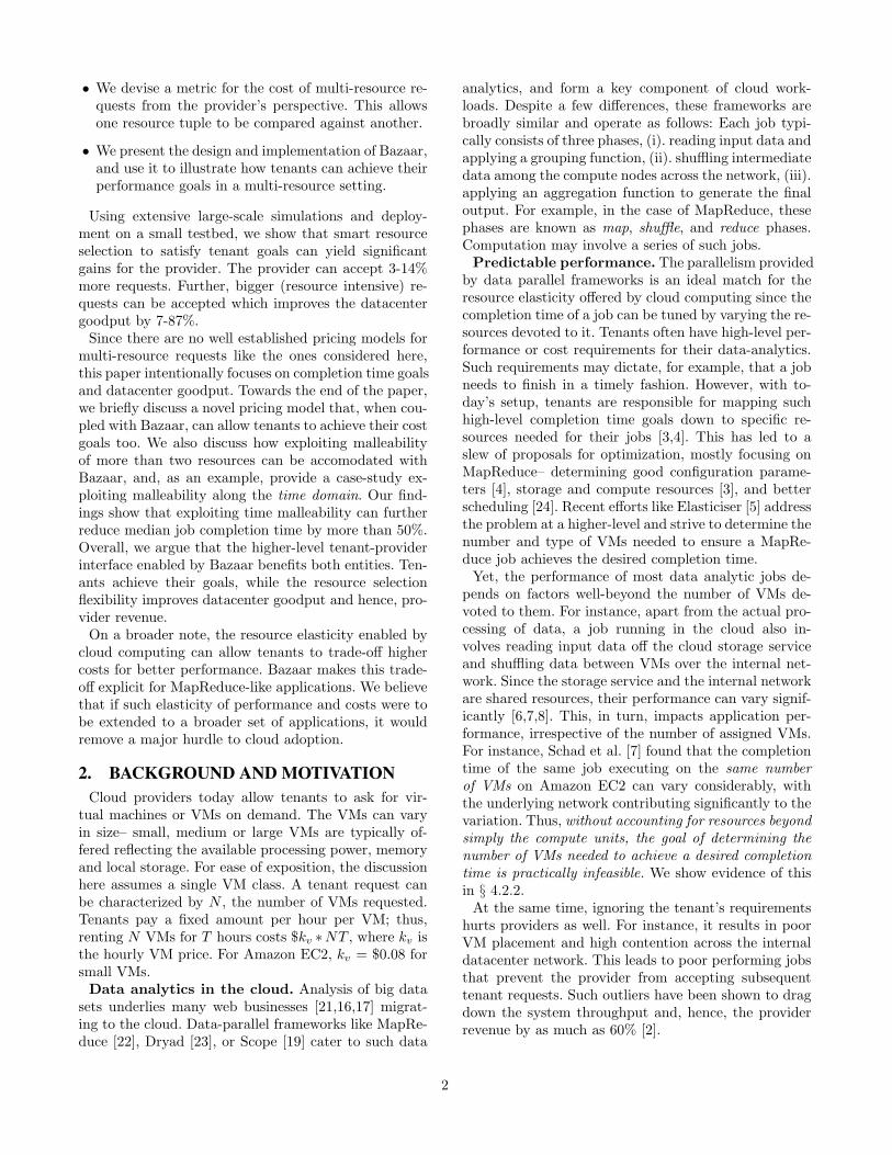
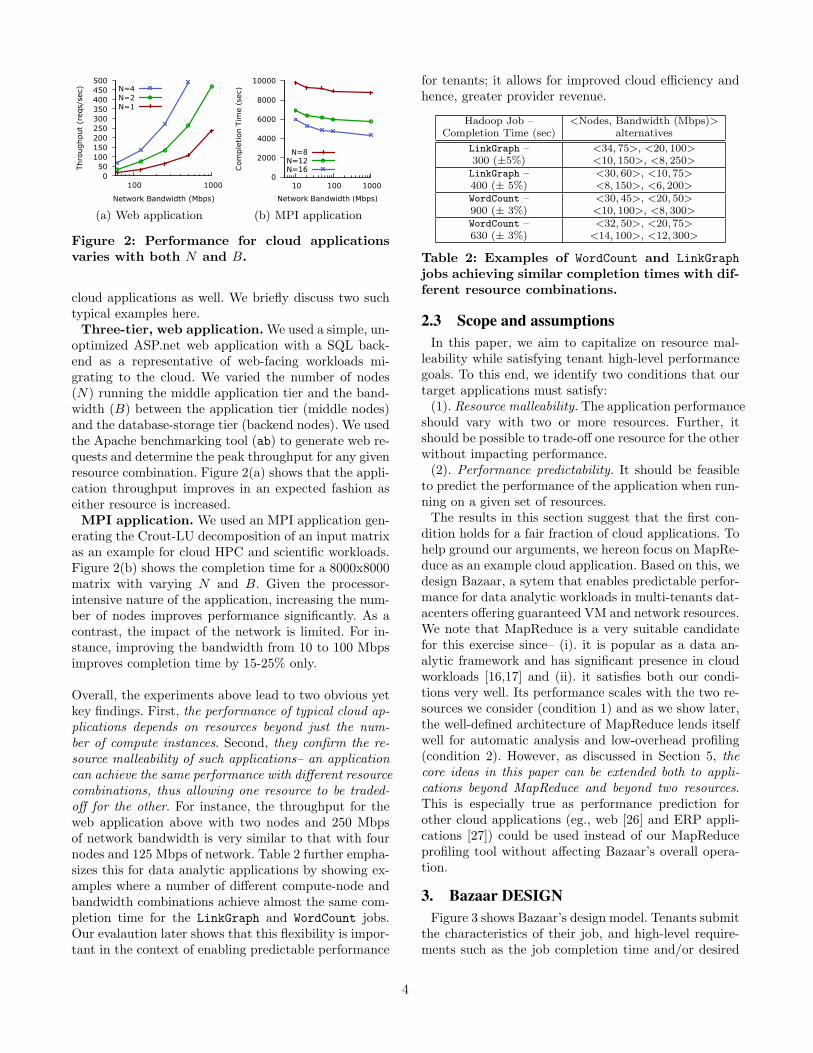
Figure 2: Performance for cloud applicationsvaries with both N and B.

cloud applications as well. We briefly discuss two suchtypical examples here.

Three-tier, web application. We used a simple, un-optimized ASP.net web application with a SQL back-end as a representative of web-facing workloads mi-grating to the cloud. We varied the number of nodes(N) running the middle application tier and the band-width (B) between the application tier (middle nodes)and the database-storage tier (backend nodes). We usedthe Apache benchmarking tool (ab) to generate web re-quests and determine the peak throughput for any givenresource combination. Figure 2(a) shows that the appli-cation throughput improves in an expected fashion aseither resource is increased.

MPI application. We used an MPI application gen-erating the Crout-LU decomposition of an input matrixas an example for cloud HPC and scientific workloads.Figure 2(b) shows the completion time for a 8000x8000matrix with varying N and B. Given the processor-intensive nature of the application, increasing the num-ber of nodes improves performance significantly. As acontrast, the impact of the network is limited. For in-stance, improving the bandwidth from 10 to 100 Mbpsimproves completion time by 15-25% only.

Overall, the experiments above lead to two obvious yetkey findings. First, the performance of typical cloud ap-plications depends on resources beyond just the num-ber of compute instances. Second, they confirm the re-source malleability of such applications– an applicationcan achieve the same performance with different resourcecombinations, thus allowing one resource to be traded-off for the other. For instance, the throughput for theweb application above with two nodes and 250 Mbpsof network bandwidth is very similar to that with fournodes and 125 Mbps of network. Table 2 further empha-sizes this for data analytic applications by showing ex-amples where a number of different compute-node andbandwidth combinations achieve almost the same com-pletion time for the LinkGraph and WordCount jobs.Our evalaution later shows that this flexibility is impor-tant in the context of enabling predictable performance

for tenants; it allows for improved cloud efficiency andhence, greater provider revenue.

Hadoop Job – <Nodes, Bandwidth (Mbps)>Completion Time (sec) alternatives

LinkGraph – <34, 75>, <20, 100>300 (±5%) <10, 150>, <8, 250>LinkGraph – <30, 60>, <10, 75>400 (± 5%) <8, 150>, <6, 200>WordCount – <30, 45>, <20, 50>900 (± 3%) <10, 100>, <8, 300>WordCount – <32, 50>, <20, 75>630 (± 3%) <14, 100>, <12, 300>

Table 2: Examples of WordCount and LinkGraphjobs achieving similar completion times with dif-ferent resource combinations.

2.3 Scope and assumptionsIn this paper, we aim to capitalize on resource mal-

leability while satisfying tenant high-level performancegoals. To this end, we identify two conditions that ourtarget applications must satisfy:

(1). Resource malleability. The application performanceshould vary with two or more resources. Further, itshould be possible to trade-off one resource for the otherwithout impacting performance.

(2). Performance predictability. It should be feasibleto predict the performance of the application when run-ning on a given set of resources.

The results in this section suggest that the first con-dition holds for a fair fraction of cloud applications. Tohelp ground our arguments, we hereon focus on MapRe-duce as an example cloud application. Based on this, wedesign Bazaar, a sytem that enables predictable perfor-mance for data analytic workloads in multi-tenants dat-acenters offering guaranteed VM and network resources.We note that MapReduce is a very suitable candidatefor this exercise since– (i). it is popular as a data an-alytic framework and has significant presence in cloudworkloads [16,17] and (ii). it satisfies both our condi-tions very well. Its performance scales with the two re-sources we consider (condition 1) and as we show later,the well-defined architecture of MapReduce lends itselfwell for automatic analysis and low-overhead profiling(condition 2). However, as discussed in Section 5, thecore ideas in this paper can be extended both to appli-cations beyond MapReduce and beyond two resources.This is especially true as performance prediction forother cloud applications (eg., web [26] and ERP appli-cations [27]) could be used instead of our MapReduceprofiling tool without affecting Bazaar’s overall opera-tion.

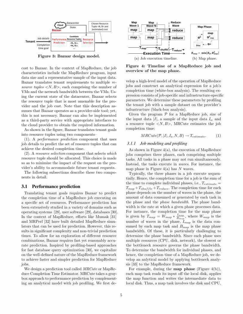
3. Bazaar DESIGNFigure 3 shows Bazaar’s design model. Tenants submit

the characteristics of their job, and high-level require-ments such as the job completion time and/or desired

4

TenantJob details

Completion time goal

PerformancePrediction

ResourceSelection

Cloud

CandidateResource Tuples

<N1, B1>, <N2, B2>,

….

Bazaar

Datacenter

State

Chosen Resource Tuple <N, B> and (estimated) cost

Figure 3: Bazaar design model.

cost to Bazaar. In the context of MapReduce, the jobcharacteristics include the MapReduce program, inputdata size and a representative sample of the input data.Bazaar translates tenant requirements to multiple re-source tuples <N,B>, each comprising the number ofVMs and the network bandwidth between the VMs. Us-ing the current state of the datacenter, Bazaar selectsthe resource tuple that is most amenable for the pro-vider and the job cost. Note that this description as-sumes that Bazaar operates as a provider-side tool; yet,this is not necessary. Bazaar can also be implementedas a third-party service with appropriate interfaces tothe cloud provider to obtain the required information.

As shown in the figure, Bazaar translates tenant goalsinto resource tuples using two components–

(1). A performance prediction component that usesjob details to predict the set of resource tuples that canachieve the desired completion time.

(2). A resource selection component that selects whichresource tuple should be allocated. This choice is madeso as to minimize the impact of the request on the pro-vider’s ability to accommodate future tenant requests.

The following subsections describe these two compo-nents in detail.

3.1 Performance predictionTranslating tenant goals requires Bazaar to predict

the completion time of a MapReduce job executing ona specific set of resources. Performance prediction hasbeen extensively studied in a variety of domains such asoperating systems [28], user software [29], databases [30].In the context of MapReduce, efforts like Mumak [31]and MRPerf [32] have built detailed MapReduce simu-lators that can be used for prediction. However, this re-sults in significant complexity and non-trivial predictiontimes. To allow for an exploration of different resourcecombinations, Bazaar requires fast yet reasonably accu-rate prediction. Inspired by profiling-based approachesfor fast database query optimization [30], we capitalizeon the well-defined nature of the MapReduce frameworkto achieve faster and simpler prediction for MapReducejobs.

We design a prediction tool called MRCute or MapRe-duce Completion Time Estimator. MRCute takes a gray-box approach to performance prediction by complement-ing an analytical model with job profiling. We first de-

Map

Wave 1

map

map

.

.

.

Map

Wave N

map

map

.

.

.

...

Reduce

Wave

Execution Time

reduce

reduce

.

.

.

Tmap Treduce Tshuffle

(a) Job execution timeline.

Map Phase

BD

map

BP

map

𝑩𝒎𝒂𝒑 = 𝐦𝐢𝐧 𝑩𝑫, 𝑩𝒎𝒂𝒑𝑷

BDDisc

(b) Map phase.

Figure 4: Timeline of a MapReduce job andoverview of the map phase.

velop a high-level model of the operation of MapReducejobs and construct an analytical expression for a job’scompletion time (white-box analysis). The resulting ex-pression consists of job-specific and infrastructure-specificparameters. We determine these parameters by profilingthe tenant job with a sample dataset on the provider’sinfrastructure (black-box analysis).

Given the program P for a MapReduce job, size ofthe input data |I|, a sample of the input data Is, anda resource tuple <N,B>, MRCute estimates the jobcompletion time:

MRCute(P, |I|, Is, N,B)→ Testimate. (1)

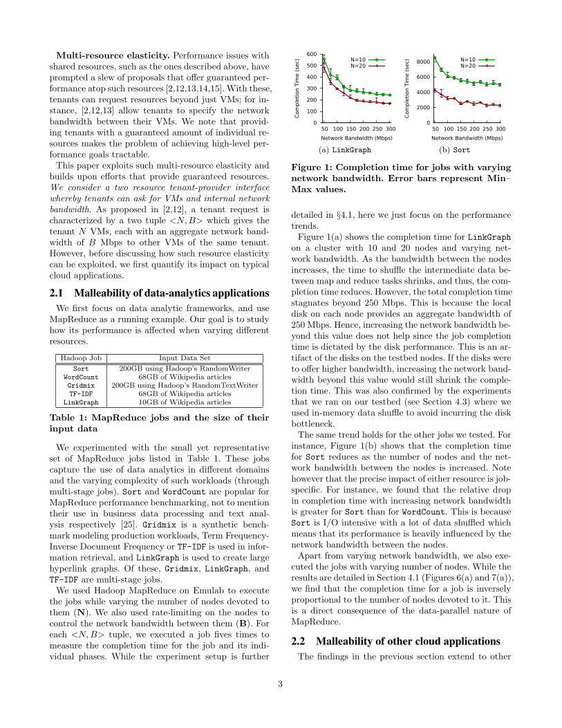
3.1.1 Job modeling and profilingAs shown in Figure 4(a), the execution of MapReduce

jobs comprises three phases, each comprising multipletasks. All tasks in a phase may not run simultaneously.Instead, the tasks execute in waves. For instance, themap phase in Figure 4(a) has N waves.

Typically, the three phases in a job execute sequen-tially. Hence, the completion time for a job is the sum ofthe time to complete individual phases, i.e., Testimate =Tmap+Tshuffle+Treduce. The completion time for eachphase depends on the number of waves in the phase, theamount of data consumed or generated by each task inthe phase and the phase bandwidth. The phase band-width is the rate at which a given phase processes data.For instance, the completion time for the map phaseis given by Tmap = Wmap ∗ Imap

Bmap, where Wmap is the

number of waves in the phase, Imap is the data con-sumed by each map task and Bmap is the map phasebandwidth. Of these, it is particularly challenging todetermine the phase bandwidth. Since each phase usesmultiple resources (CPU, disk, network), the slowest orthe bottleneck resource governs the phase bandwidth.To determine the bandwidth for individual phases, andhence, the completion time of a MapReduce job, we de-velop an anlytical model by applying bottleneck analy-sis [33] to the MapReduce framework.

For example, during the map phase (Figure 4(b)),each map task reads its input off the local disk, appliesthe map function and writes the intermediate data tolocal disk. Thus, a map task involves the disk and CPU,

5

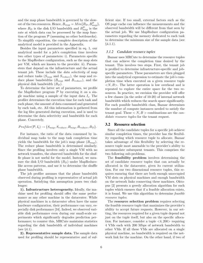
and the map phase bandwidth is governed by the slow-est of the two resources. Hence,Bmap = Min{BD, BPmap},where BD is the disk I/O bandwidth and BPmap is therate at which data can be processed by the map func-tion of the program P (assuming no other bottlenecks).To simplify exposition, the complete description of theanalytical model is provided in the Appendix.

Besides the input parameters specified in eq. 1, ouranalytical model for a job’s completion time involvestwo other types of parameters: i). Parameters specificto the MapReduce configuration, such as the map slotsper VM, which are known to the provider. ii). Param-eters that depend on the infrastructure and the actualtenant job. These include the data selectivity of mapand reduce tasks (Smap and Sreduce), the map and re-duce phase bandwidths (Bmap and Breduce), and thephysical disk bandwidth (BD).

To determine the latter set of parameters, we profilethe MapReduce program P by executing it on a sin-gle machine using a sample of the input data Is. Theprofiler determines the execution time for each task andeach phase, the amount of data consumed and generatedby each task, etc. All this information is gathered fromthe log files generated during execution, and is used todetermine the data selectivity and bandwidth for eachphase. Concretely,

Profiler(P, Is)→ {Smap, Sreduce, Bmap, Breduce, BD}.

For instance, the ratio of the data consumed by in-dividual map tasks to the map task completion timeyields the bandwidth for the job’s map phase (Bmap).The reduce phase bandwidth is determined similarly.Since the profiling involves only a single VM with nonetwork transfers, the observed bandwidth for the shuf-fle phase is not useful for the model. Instead, we mea-sure the disk I/O bandwidth (BD) under MapReduce-like access patterns, and use it to determine the shufflephase bandwidth.

The job profiler assumes that the phase bandwidthobserved during profiling is representative of actual joboperation. Satisfying this assumption poses two chal-lenges:

1). Infrastructure heterogeneity. Ideally, the ma-chine used for profiling should offer the same perfor-mance as any other machine in the datacenter. Whilephysical machines in a datacenter often have the samehardware configuration, their performance can vary, es-pecially disk performance [34]. Indeed, we observed vari-able disk performance even during our small-scale ex-periments which significantly degrades prediction per-formance; to counter this, MRCute maintains statisticsregarding the disk bandwidth of individual machines(see §4.1).

2). Representative sample data. The sample dataused for profiling should be representative and of suf-

ficient size. If too small, external factors such as theOS page cache can influence the measurements and theobserved bandwidth will be different from that seen bythe actual job. We use MapReduce configuration pa-rameters regarding the memory dedicated to each taskto determine the minimum size of the sample data (see§4.1.1).

3.1.2 Candidate resource tuplesBazaar uses MRCute to determine the resource tuples

that can achieve the completion time desired by thetenant. This involves two steps. First, the tenant jobis profiled to determine infrastructure-specific and job-specific parameters. These parameters are then pluggedinto the analytical expression to estimate the job’s com-pletion time when executed on a given resource tuple<N,B>. The latter operation is low overhead and isrepeated to explore the entire space for the two re-sources. In practice, we envision the provider will offera few classes (in the order of 10-20) of internal networkbandwidth which reduces the search space significantly.For each possible bandwidth class, Bazaar determinesthe number of compute instances needed to satisfy thetenant goal. These < N,B > combinations are the can-didate resource tuples for the tenant request.

3.2 Resource selectionSince all the candidate tuples for a specific job achieve

similar completion times, the provider has the flexibil-ity regarding which resource tuple to allocate. Bazaartakes advantage of this flexibility by selecting the re-source tuple most amenable to the provider’s ability toaccommodate subsequent tenants. This comprises thetwo following sub-problems.

The feasibility problem involves determining theset of candidate resource tuples that can actually beallocated in the datacenter, given its current utiliza-tion. For our two dimensional resource tuples, this re-quires ensuring that there are both enough unoccupiedVM slots on physical machines and enough bandwidthon the network links connecting these machines. Okto-pus [2] presents a greedy allocation algorithm for suchtuples which ensures that if a feasible allocation exists,it is found. We use this algorithm to determine feasibleresource tuples.

The resource selection problem requires selectingthe feasible resource tuple that maximizes the provider’sability to accept future requests. However, in our set-ting, the resources required for a given tuple depend notjust on the tuple itself, but also on the specific alloca-tion. For instance, consider a tuple <4, 200> requiring4 VMs each with 200 Mbps of network bandwidth toother VMs. If all these VMs are allocated on a singlephysical machine, no bandwidth is required on the net-work link for the machine. On the other hand, if two of

6

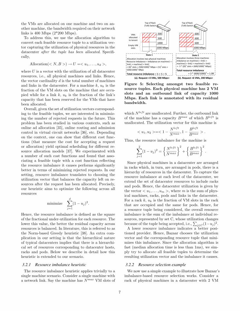
the VMs are allocated on one machine and two on an-other machine, the bandwidth required on their networklinks is 400 Mbps (2*200 Mbps).

To address this, we use the allocation algorithm toconvert each feasible resource tuple to a utilization vec-tor capturing the utilization of physical resources in thedatacenter after the tuple has been allocated. Specifi-cally,

Allocation(< N,B >)→ U =< u1, . . . , ud >,

where U is a vector with the utilization of all datacenterresources, i.e., all physical machines and links. Hence,the vector cardinality d is the total number of machinesand links in the datacenter. For a machine k, uk is thefraction of the VM slots on the machine that are occu-pied while for a link k, uk is the fraction of the link’scapacity that has been reserved for the VMs that havebeen allocated.

Overall, given the set of utilization vectors correspond-ing to the feasible tuples, we are interested in minimiz-ing the number of rejected requests in the future. Thisproblem has been studied in various contexts, such asonline ad allocation [35], online routing and admissioncontrol in virtual circuit networks [36], etc. Dependingon the context, one can show that different cost func-tions (that measure the cost for accepting a requestor allocation) yield optimal scheduling for different re-source allocation models [37]. We experimented witha number of such cost functions and found that asso-ciating a feasible tuple with a cost function reflectingthe resource imbalance it causes performs significantlybetter in terms of minimizing rejected requests. In oursetting, resource imbalance translates to choosing theutilization vector that balances the capacity left on re-sources after the request has been allocated. Precisely,our heuristic aims to optimize the following across allresources

minimized∑j=1

(1− uj)2.

Hence, the resource imbalance is defined as the squareof the fractional under-utilization for each resource. Thelower this value, the better the residual capacity acrossresources is balanced. In literature, this is referred to asthe Norm-based Greedy heuristic [38]. An extra com-plication in our setting is that the hierarchical natureof typical datacenters implies that there is a hierarchi-cal set of resources corresponding to datacenter hosts,racks and pods. Below we describe in detail how thisheuristic is extended to our scenario.

3.2.1 Resource imbalance heuristicThe resource imbalance heuristic applies trivially to a

single machine scenario. Consider a single machine witha network link. Say the machine has Nmax VM slots of

600

600

1000 Mbps

600500

500

1000

1000 Mbps

State 1

Allocation involves two physical machinesResource Imbalance = Imbalance on machine1 + link1 + machine2 + link2= (0)2 slots + (500/1000)2 Mbps + (½)2 slots + (500/1000)2 Mbps

Total resource imbalance = ¼ + ½ = ¾

VMs allocated to tenant

Empty VM slots

Top of Rack(ToR) Switch

Top of Rack(ToR) Switch

(a). Request <3 VMs, 500 Mbps> (b). Request <6 VMs, 200 Mbps>

State 2Allocation involves three machinesImbalance on machine1 + link1 + machine2 + link2 + machine3 + link3 = 3 * {(0)2 slots + (600/1000)2 Mbps}

Total resource imbalance = 3 * (600/1000)2 = 1.08

Figure 5: Selecting amongst two feasible re-source tuples. Each physical machine has 2 VMslots and an outbound link of capacity 1000Mbps. Each link is annotated with its residualbandwidth.

which N left are unallocated. Further, the outbound linkof the machine has a capacity Bmax of which Bleft isunallocated. The utilization vector for this machine is

< u1, u2 >=< 1− N left

Nmax, 1− Bleft

Bmax> .

Thus, the resource imbalance for the machine is

2∑j=1

(1− uj)2 ={N left

Nmax

}2

+{Bleft

Bmax

}2

.

Since physical machines in a datacenter are arrangedin racks which, in turn, are arranged in pods, there is ahierarchy of resources in the datacenter. To capture theresource imbalance at each level of the datacenter, weextend the set of datacenter resources to include racksand pods. Hence, the datacenter utilization is given bythe vector < u1, . . . , um >, where m is the sum of phys-ical machines, racks, pods and links in the datacenter.For a rack k, uk is the fraction of VM slots in the rackthat are occupied and the same for pods. Hence, fora resource tuple being considered, the overall resourceimbalance is the sum of the imbalance at individual re-sources, represented by set C, whose utilization changesbecause of the tuple being accepted, i.e.,

∑j∈C(1−uj)2.

A lower resource imbalance indicates a better posi-tioned provider. Hence, Bazaar chooses the utilizationvector and the corresponding resource tuple that mini-mizes this imbalance. Since the allocation algorithm isfast (median allocation time is less than 1ms), we sim-ply try to allocate all feasible tuples to determine theresulting utilization vector and the imbalance it causes.

3.2.2 Resource selection exampleWe now use a simple example to illustrate how Bazaar’s

imbalance-based resource selection works. Consider arack of physical machines in a datacenter with 2 VM

7

slots and a Gigabit link per machine. Also, imagine atenant request with two feasible tuples <N,B> (B inMbps): <3, 500> and <6, 200>. Figure 5 shows allo-cations for these two resource tuples. Network links inthe figure are annotated with the (unreserved) residualbandwidth on the link after the allocation. The figurealso shows the imbalance values for the resulting data-center states. The former tuple has a lower imbalanceand is chosen by Bazaar.

To understand this choice, we focus on the resourcesleft in the datacenter after the allocations. After theallocation of the <3, 500> tuple, the provider is leftwith five empty VM slots, each with an average net-work bandwidth of 500 Mbps (state-1). As a contrast,the allocation of <6, 200> results in two empty VMslots, again with an average network bandwidth of 500Mbps (state-2). We note that any subsequent tenantrequest that can be accommodated by the provider instate-2 can also be accommodated in state-1. However,the reverse is not true. For instance, a future tenant re-quiring the tuple <3, 400> can be allocated in state-1but not state-2. Hence, the first tuple is more desirablefor the provider and is the one chosen by the resourceimbalance metric.

4. EVALUATIONIn this section, we evaluate Bazaar focusing on its twomain components, namely MRCute, and resource selec-tion. Our evaluation combines MapReduce experiments,simulations and a testbed deployment. Specifically:

(1). We quantify the accuracy of MRCute. Resultsindicate that MRCute accurately determines the re-sources required to achieve tenant goals with low over-head and an average prediction error of less than 12%(§4.1).

(2). We use large scale simulations to evaluate thebenefits of Bazaar. Capitalizing on resource malleabilitysignificantly improves datacenter goodput (§4.2).

(3). We deploy and benchmark our prototype on asmall scale 26-node cluster. We further use this deploy-ment to cross-validate our simulation results (§4.3).

4.1 Performance predictionWe use MRCute to predict the job completion of the

five MapReduce jobs described in §2.1 (Table 1). Foreach job, MRCute predicts the completion time for vary-ing number of nodes (N) and the network bandwidthbetween them (B). As detailed in §3.1, the predictioninvolves profiling the job with sample data on a singlenode, and using the resulting job parameters to drivethe analytical model.

To determine actual completion times, we executedeach job on a 35-node Emulab cluster with Cloudera’sdistribution of Hadoop MapReduce. Each node has aquad-core Intel Xeon 2.4GHz processor, 12 GB RAM

0

4000

8000

12000

16000

20000

24000

4 8 12 16 20 24 28 32

Com

ple

tion T

ime (

sec)

Number of nodes

50Mbps (obs)50Mbps (pred)300Mbps (obs)

300Mbps (pred)

(a) Varying Nodes

0

2000

4000

6000

8000

10000

12000

50 100 150 200 250 300

Com

ple

tion

Tim

e (

sec)

Network Bandwidth (Mbps)

N=10 (obs)N=10 (pred)N=20 (obs)

N=20 (pred)

(b) Varying Bandwidth

Figure 6: Predicted completion time for Sort, anI/O intensive job, matches the observed time.

0

500

1000

1500

2000

2500

3000

4 8 12 16 20 24 28 32

Com

ple

tion T

ime (

sec)

Number of nodes

50Mbps (obs)50Mbps (pred)300Mbps (obs)

300Mbps (pred)

(a) Varying Nodes

0

200

400

600

800

1000

1200

1400

1600

50 100 150 200 250 300

Com

ple

tion

Tim

e (

sec)

Network Bandwidth (Mbps)

N=10 (obs)N=10 (pred)N=20 (obs)

N=20 (pred)

(b) Varying Bandwidth

Figure 7: Predicted completion time for Word-Count, a processing intensive job, matches theobserved time.

and a 1Gbps network interface. The unoptimized jobswere run with default Hadoop configuration parameters.The number of mappers and reducers per node is 8 and2 respectively, HDFS block size is 128 MB, and the to-tal number of reducers is twice the number of nodesused. While parameter tuning can improve job perfor-mance significantly [5], our focus here is not improvingindividual jobs, but rather predicting the performancefor a given configuration. Hence, the results presentedhere apply as long as the same parameters are used forjob profiling and for the actual execution. In the nextparagraphs, we examine in detail the prediction resultsof the various jobs, and the factors introducing errorsin our model.

We first focus on the results for Sort and WordCount,two jobs at extreme ends of the spectrum. Sort is anI/O intensive job while WordCount is processor inten-sive. Figures 6 and 7 plot the observed and predictedcompletion time for five runs of these jobs when vary-ing N and B. The figures show that the predicted andobserved completion times are close throughout, with8.9% prediction error on average for Sort and 20.5% atthe 95th percentile.

To understand the root cause of the prediction er-rors, we look at the per-phase completion time. Fig-ure 8 presents this breakdown for Sort with varyingnumber of nodes. The bars labeled Obs and Pred rep-resent the observed and predicted completion time re-spectively. The figure shows that the predicted time for

8

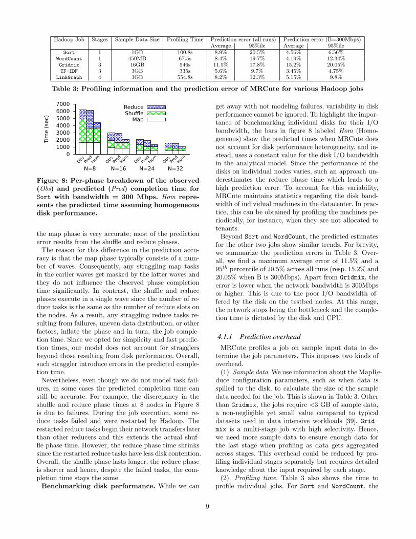
Hadoop Job Stages Sample Data Size Profiling Time Prediction error (all runs) Prediction error (B=300Mbps)Average 95%ile Average 95%ile

Sort 1 1GB 100.8s 8.9% 20.5% 4.56% 6.56%WordCount 1 450MB 67.5s 8.4% 19.7% 4.19% 12.34%Gridmix 3 16GB 546s 11.5% 17.8% 15.2% 20.05%TF-IDF 3 3GB 335s 5.6% 9.7% 3.45% 4.75%

LinkGraph 4 3GB 554.8s 8.2% 12.3% 5.15% 9.8%

Table 3: Profiling information and the prediction error of MRCute for various Hadoop jobs

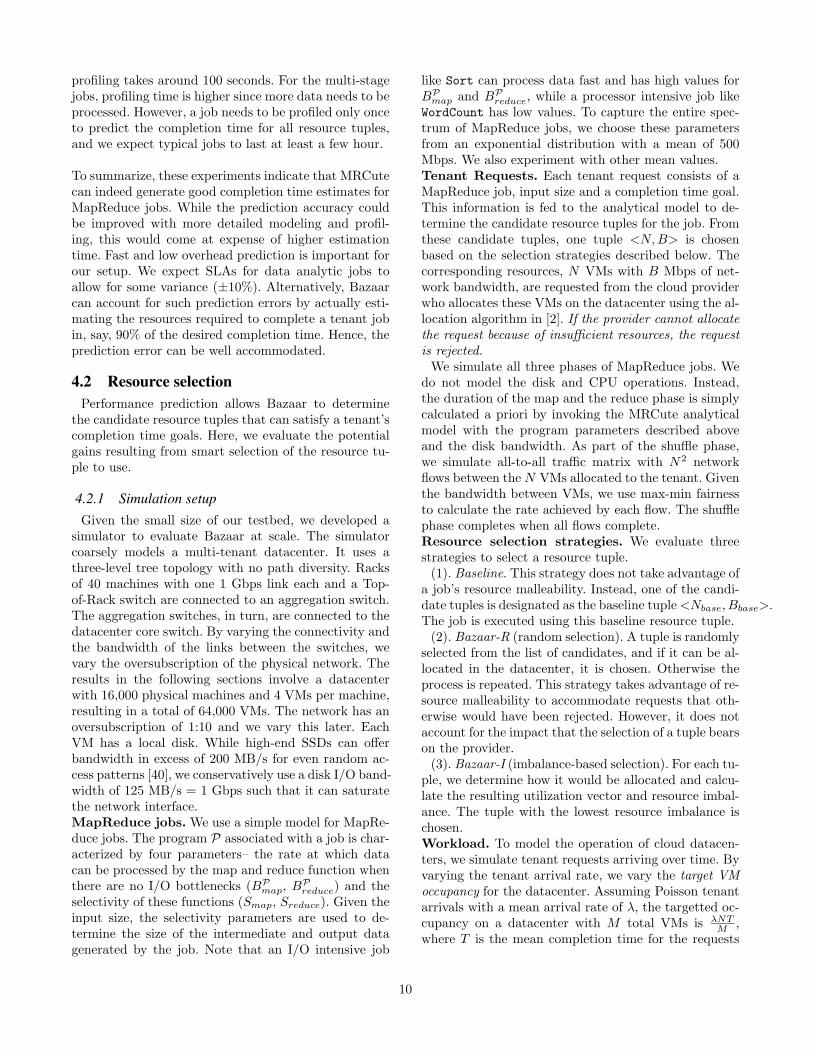
0 1000 2000 3000 4000 5000 6000 7000

Obs Pred

Hom Obs Pred

Hom Obs Pred

Hom Obs Pred

Hom

Tim

e (

sec)

ReduceShuffle

Map

N=32N=24N=16N=8

Figure 8: Per-phase breakdown of the observed(Obs) and predicted (Pred) completion time forSort with bandwidth = 300 Mbps. Hom repre-sents the predicted time assuming homogeneousdisk performance.

the map phase is very accurate; most of the predictionerror results from the shuffle and reduce phases.

The reason for this difference in the prediction accu-racy is that the map phase typically consists of a num-ber of waves. Consequently, any straggling map tasksin the earlier waves get masked by the latter waves andthey do not influence the observed phase completiontime significantly. In contrast, the shuffle and reducephases execute in a single wave since the number of re-duce tasks is the same as the number of reduce slots onthe nodes. As a result, any straggling reduce tasks re-sulting from failures, uneven data distribution, or otherfactors, inflate the phase and in turn, the job comple-tion time. Since we opted for simplicity and fast predic-tion times, our model does not account for stragglersbeyond those resulting from disk performance. Overall,such straggler introduce errors in the predicted comple-tion time.

Nevertheless, even though we do not model task fail-ures, in some cases the predicted completion time canstill be accurate. For example, the discrepancy in theshuffle and reduce phase times at 8 nodes in Figure 8is due to failures. During the job execution, some re-duce tasks failed and were restarted by Hadoop. Therestarted reduce tasks begin their network transfers laterthan other reducers and this extends the actual shuf-fle phase time. However, the reduce phase time shrinkssince the restarted reduce tasks have less disk contention.Overall, the shuffle phase lasts longer, the reduce phaseis shorter and hence, despite the failed tasks, the com-pletion time stays the same.

Benchmarking disk performance. While we can

get away with not modeling failures, variability in diskperformance cannot be ignored. To highlight the impor-tance of benchmarking individual disks for their I/Obandwidth, the bars in figure 8 labeled Hom (Homo-geneous) show the predicted times when MRCute doesnot account for disk performance heterogeneity, and in-stead, uses a constant value for the disk I/O bandwidthin the analytical model. Since the performance of thedisks on individual nodes varies, such an approach un-derestimates the reduce phase time which leads to ahigh prediction error. To account for this variability,MRCute maintains statistics regarding the disk band-width of individual machines in the datacenter. In prac-tice, this can be obtained by profiling the machines pe-riodically, for instance, when they are not allocated totenants.

Beyond Sort and WordCount, the predicted estimatesfor the other two jobs show similar trends. For brevity,we summarize the prediction errors in Table 3. Over-all, we find a maximum average error of 11.5% and a95th percentile of 20.5% across all runs (resp. 15.2% and20.05% when B is 300Mbps). Apart from Gridmix, theerror is lower when the network bandwidth is 300Mbpsor higher. This is due to the poor I/O bandwidth of-fered by the disk on the testbed nodes. At this range,the network stops being the bottleneck and the comple-tion time is dictated by the disk and CPU.

4.1.1 Prediction overheadMRCute profiles a job on sample input data to de-

termine the job parameters. This imposes two kinds ofoverhead.

(1). Sample data. We use information about the MapRe-duce configuration parameters, such as when data isspilled to the disk, to calculate the size of the sampledata needed for the job. This is shown in Table 3. Otherthan Gridmix, the jobs require <3 GB of sample data,a non-negligible yet small value compared to typicaldatasets used in data intensive workloads [39]. Grid-mix is a multi-stage job with high selectivity. Hence,we need more sample data to ensure enough data forthe last stage when profiling as data gets aggregatedacross stages. This overhead could be reduced by pro-filing individual stages separately but requires detailedknowledge about the input required by each stage.

(2). Profiling time. Table 3 also shows the time toprofile individual jobs. For Sort and WordCount, the

9

profiling takes around 100 seconds. For the multi-stagejobs, profiling time is higher since more data needs to beprocessed. However, a job needs to be profiled only onceto predict the completion time for all resource tuples,and we expect typical jobs to last at least a few hour.

To summarize, these experiments indicate that MRCutecan indeed generate good completion time estimates forMapReduce jobs. While the prediction accuracy couldbe improved with more detailed modeling and profil-ing, this would come at expense of higher estimationtime. Fast and low overhead prediction is important forour setup. We expect SLAs for data analytic jobs toallow for some variance (±10%). Alternatively, Bazaarcan account for such prediction errors by actually esti-mating the resources required to complete a tenant jobin, say, 90% of the desired completion time. Hence, theprediction error can be well accommodated.

4.2 Resource selectionPerformance prediction allows Bazaar to determine

the candidate resource tuples that can satisfy a tenant’scompletion time goals. Here, we evaluate the potentialgains resulting from smart selection of the resource tu-ple to use.

4.2.1 Simulation setupGiven the small size of our testbed, we developed a

simulator to evaluate Bazaar at scale. The simulatorcoarsely models a multi-tenant datacenter. It uses athree-level tree topology with no path diversity. Racksof 40 machines with one 1 Gbps link each and a Top-of-Rack switch are connected to an aggregation switch.The aggregation switches, in turn, are connected to thedatacenter core switch. By varying the connectivity andthe bandwidth of the links between the switches, wevary the oversubscription of the physical network. Theresults in the following sections involve a datacenterwith 16,000 physical machines and 4 VMs per machine,resulting in a total of 64,000 VMs. The network has anoversubscription of 1:10 and we vary this later. EachVM has a local disk. While high-end SSDs can offerbandwidth in excess of 200 MB/s for even random ac-cess patterns [40], we conservatively use a disk I/O band-width of 125 MB/s = 1 Gbps such that it can saturatethe network interface.MapReduce jobs. We use a simple model for MapRe-duce jobs. The program P associated with a job is char-acterized by four parameters– the rate at which datacan be processed by the map and reduce function whenthere are no I/O bottlenecks (BPmap, B

Preduce) and the

selectivity of these functions (Smap, Sreduce). Given theinput size, the selectivity parameters are used to de-termine the size of the intermediate and output datagenerated by the job. Note that an I/O intensive job

like Sort can process data fast and has high values forBPmap and BPreduce, while a processor intensive job likeWordCount has low values. To capture the entire spec-trum of MapReduce jobs, we choose these parametersfrom an exponential distribution with a mean of 500Mbps. We also experiment with other mean values.Tenant Requests. Each tenant request consists of aMapReduce job, input size and a completion time goal.This information is fed to the analytical model to de-termine the candidate resource tuples for the job. Fromthese candidate tuples, one tuple <N,B> is chosenbased on the selection strategies described below. Thecorresponding resources, N VMs with B Mbps of net-work bandwidth, are requested from the cloud providerwho allocates these VMs on the datacenter using the al-location algorithm in [2]. If the provider cannot allocatethe request because of insufficient resources, the requestis rejected.

We simulate all three phases of MapReduce jobs. Wedo not model the disk and CPU operations. Instead,the duration of the map and the reduce phase is simplycalculated a priori by invoking the MRCute analyticalmodel with the program parameters described aboveand the disk bandwidth. As part of the shuffle phase,we simulate all-to-all traffic matrix with N2 networkflows between the N VMs allocated to the tenant. Giventhe bandwidth between VMs, we use max-min fairnessto calculate the rate achieved by each flow. The shufflephase completes when all flows complete.Resource selection strategies. We evaluate threestrategies to select a resource tuple.

(1). Baseline. This strategy does not take advantage ofa job’s resource malleability. Instead, one of the candi-date tuples is designated as the baseline tuple<Nbase, Bbase>.The job is executed using this baseline resource tuple.

(2). Bazaar-R (random selection). A tuple is randomlyselected from the list of candidates, and if it can be al-located in the datacenter, it is chosen. Otherwise theprocess is repeated. This strategy takes advantage of re-source malleability to accommodate requests that oth-erwise would have been rejected. However, it does notaccount for the impact that the selection of a tuple bearson the provider.

(3). Bazaar-I (imbalance-based selection). For each tu-ple, we determine how it would be allocated and calcu-late the resulting utilization vector and resource imbal-ance. The tuple with the lowest resource imbalance ischosen.Workload. To model the operation of cloud datacen-ters, we simulate tenant requests arriving over time. Byvarying the tenant arrival rate, we vary the target VMoccupancy for the datacenter. Assuming Poisson tenantarrivals with a mean arrival rate of λ, the targetted oc-cupancy on a datacenter with M total VMs is λNT

M ,where T is the mean completion time for the requests

10

0

5

10

15

20

25

30

10 25 50 75 100

Rej

ecte

d r

eques

ts (

%)

Target Occupancy (%)

BaselineBazaar-RBazaar-I

(a) Mean BW = 500Mbps

0

5

10

15

20

25

30

100 300 500 700 900

Rej

ecte

d r

eques

ts (

%)

Bandwidth (Mbps)

BaselineBazaar-RBazaar-I

(b) Target Occupancy = 75%

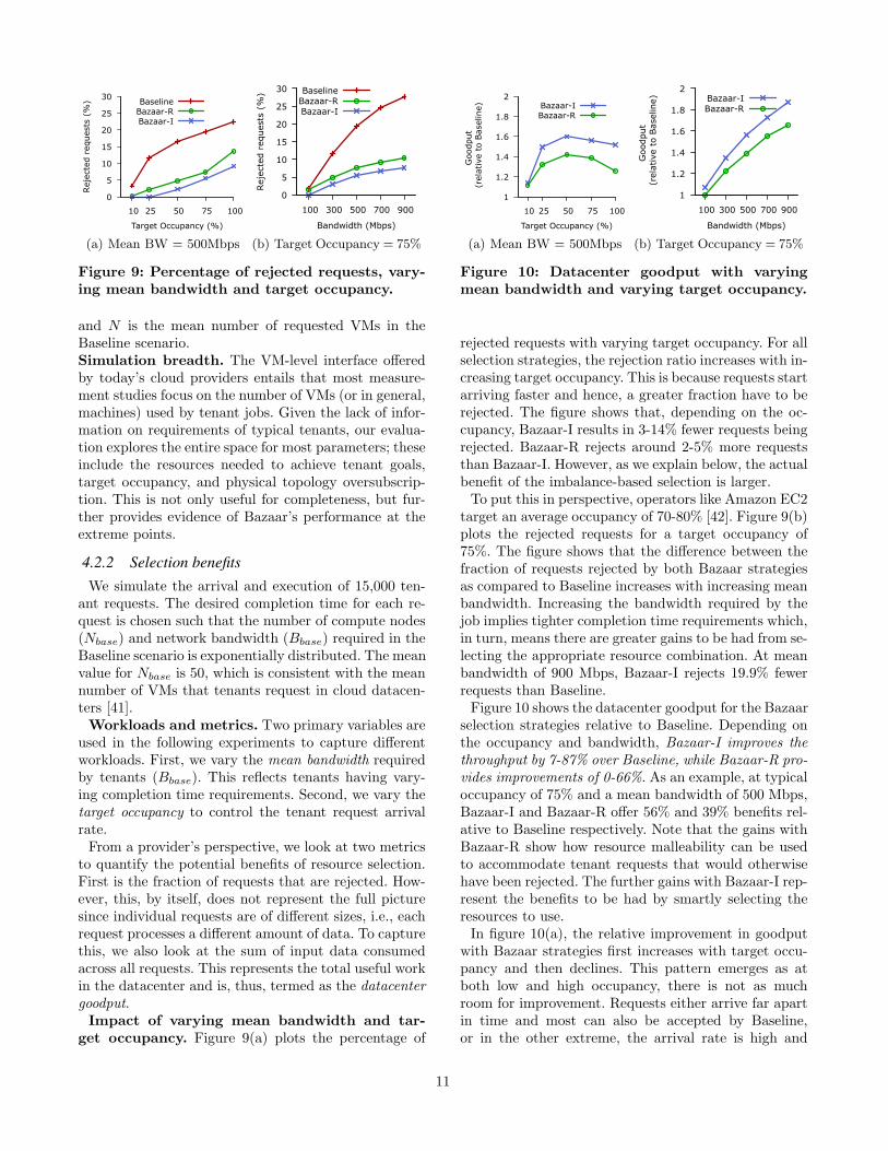
Figure 9: Percentage of rejected requests, vary-ing mean bandwidth and target occupancy.

and N is the mean number of requested VMs in theBaseline scenario.Simulation breadth. The VM-level interface offeredby today’s cloud providers entails that most measure-ment studies focus on the number of VMs (or in general,machines) used by tenant jobs. Given the lack of infor-mation on requirements of typical tenants, our evalua-tion explores the entire space for most parameters; theseinclude the resources needed to achieve tenant goals,target occupancy, and physical topology oversubscrip-tion. This is not only useful for completeness, but fur-ther provides evidence of Bazaar’s performance at theextreme points.

4.2.2 Selection benefitsWe simulate the arrival and execution of 15,000 ten-

ant requests. The desired completion time for each re-quest is chosen such that the number of compute nodes(Nbase) and network bandwidth (Bbase) required in theBaseline scenario is exponentially distributed. The meanvalue for Nbase is 50, which is consistent with the meannumber of VMs that tenants request in cloud datacen-ters [41].

Workloads and metrics. Two primary variables areused in the following experiments to capture differentworkloads. First, we vary the mean bandwidth requiredby tenants (Bbase). This reflects tenants having vary-ing completion time requirements. Second, we vary thetarget occupancy to control the tenant request arrivalrate.

From a provider’s perspective, we look at two metricsto quantify the potential benefits of resource selection.First is the fraction of requests that are rejected. How-ever, this, by itself, does not represent the full picturesince individual requests are of different sizes, i.e., eachrequest processes a different amount of data. To capturethis, we also look at the sum of input data consumedacross all requests. This represents the total useful workin the datacenter and is, thus, termed as the datacentergoodput.

Impact of varying mean bandwidth and tar-get occupancy. Figure 9(a) plots the percentage of

1

1.2

1.4

1.6

1.8

2

10 25 50 75 100

Goo

dput

(re

lative

to

Bas

elin

e)

Target Occupancy (%)

Bazaar-IBazaar-R

(a) Mean BW = 500Mbps

1

1.2

1.4

1.6

1.8

2

100 300 500 700 900

Goo

dput

(re

lative

to

Bas

elin

e)

Bandwidth (Mbps)

Bazaar-IBazaar-R

(b) Target Occupancy = 75%

Figure 10: Datacenter goodput with varyingmean bandwidth and varying target occupancy.

rejected requests with varying target occupancy. For allselection strategies, the rejection ratio increases with in-creasing target occupancy. This is because requests startarriving faster and hence, a greater fraction have to berejected. The figure shows that, depending on the oc-cupancy, Bazaar-I results in 3-14% fewer requests beingrejected. Bazaar-R rejects around 2-5% more requeststhan Bazaar-I. However, as we explain below, the actualbenefit of the imbalance-based selection is larger.

To put this in perspective, operators like Amazon EC2target an average occupancy of 70-80% [42]. Figure 9(b)plots the rejected requests for a target occupancy of75%. The figure shows that the difference between thefraction of requests rejected by both Bazaar strategiesas compared to Baseline increases with increasing meanbandwidth. Increasing the bandwidth required by thejob implies tighter completion time requirements which,in turn, means there are greater gains to be had from se-lecting the appropriate resource combination. At meanbandwidth of 900 Mbps, Bazaar-I rejects 19.9% fewerrequests than Baseline.

Figure 10 shows the datacenter goodput for the Bazaarselection strategies relative to Baseline. Depending onthe occupancy and bandwidth, Bazaar-I improves thethroughput by 7-87% over Baseline, while Bazaar-R pro-vides improvements of 0-66%. As an example, at typicaloccupancy of 75% and a mean bandwidth of 500 Mbps,Bazaar-I and Bazaar-R offer 56% and 39% benefits rel-ative to Baseline respectively. Note that the gains withBazaar-R show how resource malleability can be usedto accommodate tenant requests that would otherwisehave been rejected. The further gains with Bazaar-I rep-resent the benefits to be had by smartly selecting theresources to use.

In figure 10(a), the relative improvement in goodputwith Bazaar strategies first increases with target occu-pancy and then declines. This pattern emerges as atboth low and high occupancy, there is not as muchroom for improvement. Requests either arrive far apartin time and most can also be accepted by Baseline,or in the other extreme, the arrival rate is high and

11

the datacenter is heavily utilized. In figure 10(b), thegains increase with increasing bandwidth. As explainedabove, this results from shrinking completion time re-quirements which allow Bazaar strategies to accept morerequests as compared to Baseline. Further, Bazaar isable to accept bigger requests resulting in even higherrelative gains.

Impact of simulation parameters. We also deter-mined the impact of other simulation parameters onBazaar performance and the results stay qualitativelythe same. Due to space constraints, we only show theresults of varying oversubscription and briefly discussthe impact of varying the mean disk and map and re-duce bandwidth below.

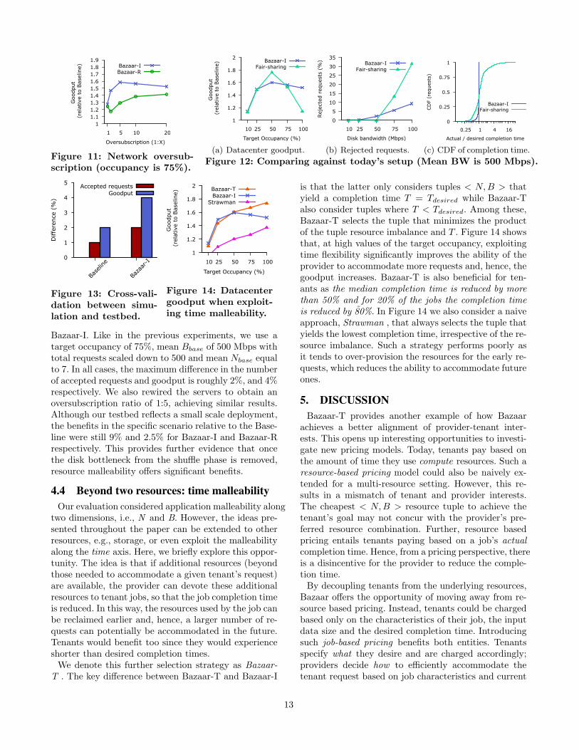
Figure 11 shows the relative goodput with varyingnetwork oversubscription. Even in a network with nooversubscription [43,44], Bazaar-I is able to accept 10%more requests and improves the goodput by 27% rela-tive to Baseline. Further, the relative improvement withBazaar increases with increasing oversubscription be-fore flattening out. This is because the physical net-work becomes more constrained and Bazaar can benefitby reducing the network requirements of tenants whileincreasing their VMs.

We also ran experiments using different values of thedisk bandwidth. As expected, low values of the diskbandwidth reduce the benefits of Bazaar-I. When thedisk bandwidth is extremely low (250 Mbps), increasingthe network bandwidth beyond this value does not im-prove performance (2% over baseline). Thus, there arevery few candidate resource tuples and the gains withBazaar are small. However, as the disk bandwidth im-proves, there are more candidate tuples to choose fromand, hence, the performance of Bazaar improves.

Finally, we varied the mean task bandwidth (map andreduce) and also the datacenter size (up to a maximumof 32,000 servers and 128,000 VMs) and the results con-firmed the trends observed in Figure 9 and 10.

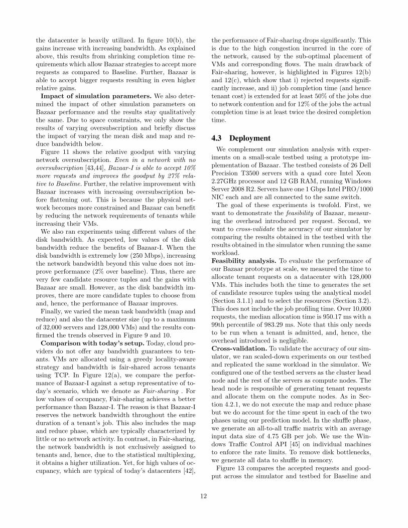
Comparison with today’s setup. Today, cloud pro-viders do not offer any bandwidth guarantees to ten-ants. VMs are allocated using a greedy locality-awarestrategy and bandwidth is fair-shared across tenantsusing TCP. In Figure 12(a), we compare the perfor-mance of Bazaar-I against a setup representative of to-day’s scenario, which we denote as Fair-sharing . Forlow values of occupancy, Fair-sharing achieves a betterperformance than Bazaar-I. The reason is that Bazaar-Ireserves the network bandwidth throughout the entireduration of a tenant’s job. This also includes the mapand reduce phase, which are typically characterized bylittle or no network activity. In contrast, in Fair-sharing,the network bandwidth is not exclusively assigned totenants and, hence, due to the statistical multiplexing,it obtains a higher utilization. Yet, for high values of oc-cupancy, which are typical of today’s datacenters [42],

the performance of Fair-sharing drops significantly. Thisis due to the high congestion incurred in the core ofthe network, caused by the sub-optimal placement ofVMs and corresponding flows. The main drawback ofFair-sharing, however, is highlighted in Figures 12(b)and 12(c), which show that i) rejected requests signifi-cantly increase, and ii) job completion time (and hencetenant cost) is extended for at least 50% of the jobs dueto network contention and for 12% of the jobs the actualcompletion time is at least twice the desired completiontime.

4.3 DeploymentWe complement our simulation analysis with exper-

iments on a small-scale testbed using a prototype im-plementation of Bazaar. The testbed consists of 26 DellPrecision T3500 servers with a quad core Intel Xeon2.27GHz processor and 12 GB RAM, running WindowsServer 2008 R2. Servers have one 1 Gbps Intel PRO/1000NIC each and are all connected to the same switch.

The goal of these experiments is twofold. First, wewant to demonstrate the feasibility of Bazaar, measur-ing the overhead introduced per request. Second, wewant to cross-validate the accuracy of our simulator bycomparing the results obtained in the testbed with theresults obtained in the simulator when running the sameworkload.Feasibility analysis. To evaluate the performance ofour Bazaar prototype at scale, we measured the time toallocate tenant requests on a datacenter with 128,000VMs. This includes both the time to generates the setof candidate resource tuples using the analytical model(Section 3.1.1) and to select the resources (Section 3.2).This does not include the job profiling time. Over 10,000requests, the median allocation time is 950.17 ms with a99th percentile of 983.29 ms. Note that this only needsto be run when a tenant is admitted, and, hence, theoverhead introduced is negligible.Cross-validation. To validate the accuracy of our sim-ulator, we ran scaled-down experiments on our testbedand replicated the same workload in the simulator. Weconfigured one of the testbed servers as the cluster headnode and the rest of the servers as compute nodes. Thehead node is responsible of generating tenant requestsand allocate them on the compute nodes. As in Sec-tion 4.2.1, we do not execute the map and reduce phasebut we do account for the time spent in each of the twophases using our prediction model. In the shuffle phase,we generate an all-to-all traffic matrix with an averageinput data size of 4.75 GB per job. We use the Win-dows Traffic Control API [45] on individual machinesto enforce the rate limits. To remove disk bottlenecks,we generate all data to shuffle in memory.

Figure 13 compares the accepted requests and good-put across the simulator and testbed for Baseline and

12

1 1.1 1.2 1.3 1.4 1.5 1.6 1.7 1.8 1.9

1 5 10 20

Goo

dput

(re

lative

to

Bas

elin

e)

Oversubscription (1:X)

Bazaar-IBazaar-R

Figure 11: Network oversub-scription (occupancy is 75%).

1

1.2

1.4

1.6

1.8

2

10 25 50 75 100

Goo

dput

(re

lative

to

Bas

elin

e)

Target Occupancy (%)

Bazaar-IFair-sharing

(a) Datacenter goodput.

0

5

10

15

20

25

30

35

10 25 50 75 100

Rej

ecte

d r

eques

ts (

%)

Disk bandwidth (Mbps)

Bazaar-IFair-sharing

(b) Rejected requests.

0

0.25

0.5

0.75

1

0.25 1 4 16

CD

F (r

eques

ts)

Actual / desired completion time

Bazaar-IFair-sharing

(c) CDF of completion time.

Figure 12: Comparing against today’s setup (Mean BW is 500 Mbps).

0

1

2

3

4

5

Base

line

Baza

ar-I

Diffe

rence

(%

)

Accepted requestsGoodput

Figure 13: Cross-vali-dation between simu-lation and testbed.

1

1.2

1.4

1.6

1.8

2

10 25 50 75 100

Goo

dput

(re

lative

to

Bas

elin

e)

Target Occupancy (%)

Bazaar-TBazaar-I

Strawman

Figure 14: Datacentergoodput when exploit-ing time malleability.

Bazaar-I. Like in the previous experiments, we use atarget occupancy of 75%, mean Bbase of 500 Mbps withtotal requests scaled down to 500 and mean Nbase equalto 7. In all cases, the maximum difference in the numberof accepted requests and goodput is roughly 2%, and 4%respectively. We also rewired the servers to obtain anoversubscription ratio of 1:5, achieving similar results.Although our testbed reflects a small scale deployment,the benefits in the specific scenario relative to the Base-line were still 9% and 2.5% for Bazaar-I and Bazaar-Rrespectively. This provides further evidence that oncethe disk bottleneck from the shuffle phase is removed,resource malleability offers significant benefits.

4.4 Beyond two resources: time malleabilityOur evaluation considered application malleability along

two dimensions, i.e., N and B. However, the ideas pre-sented throughout the paper can be extended to otherresources, e.g., storage, or even exploit the malleabilityalong the time axis. Here, we briefly explore this oppor-tunity. The idea is that if additional resources (beyondthose needed to accommodate a given tenant’s request)are available, the provider can devote these additionalresources to tenant jobs, so that the job completion timeis reduced. In this way, the resources used by the job canbe reclaimed earlier and, hence, a larger number of re-quests can potentially be accommodated in the future.Tenants would benefit too since they would experienceshorter than desired completion times.

We denote this further selection strategy as Bazaar-T . The key difference between Bazaar-T and Bazaar-I

is that the latter only considers tuples < N,B > thatyield a completion time T = Tdesired while Bazaar-Talso consider tuples where T < Tdesired. Among these,Bazaar-T selects the tuple that minimizes the productof the tuple resource imbalance and T . Figure 14 showsthat, at high values of the target occupancy, exploitingtime flexibility significantly improves the ability of theprovider to accommodate more requests and, hence, thegoodput increases. Bazaar-T is also beneficial for ten-ants as the median completion time is reduced by morethan 50% and for 20% of the jobs the completion timeis reduced by 80%. In Figure 14 we also consider a naiveapproach, Strawman , that always selects the tuple thatyields the lowest completion time, irrespective of the re-source imbalance. Such a strategy performs poorly asit tends to over-provision the resources for the early re-quests, which reduces the ability to accommodate futureones.

5. DISCUSSIONBazaar-T provides another example of how Bazaar

achieves a better alignment of provider-tenant inter-ests. This opens up interesting opportunities to investi-gate new pricing models. Today, tenants pay based onthe amount of time they use compute resources. Such aresource-based pricing model could also be naively ex-tended for a multi-resource setting. However, this re-sults in a mismatch of tenant and provider interests.The cheapest < N,B > resource tuple to achieve thetenant’s goal may not concur with the provider’s pre-ferred resource combination. Further, resource basedpricing entails tenants paying based on a job’s actualcompletion time. Hence, from a pricing perspective, thereis a disincentive for the provider to reduce the comple-tion time.

By decoupling tenants from the underlying resources,Bazaar offers the opportunity of moving away from re-source based pricing. Instead, tenants could be chargedbased only on the characteristics of their job, the inputdata size and the desired completion time. Introducingsuch job-based pricing benefits both entities. Tenantsspecify what they desire and are charged accordingly;providers decide how to efficiently accommodate thetenant request based on job characteristics and current

13

datacenter utilization. Further, since the final price doesnot depend on the completion time, providers now havean incentive to complete tenant jobs on time, possiblyeven earlier than the desired time as in Bazaar-T.

Bazaar, when combined with job-based pricing, canenable a symbiotic tenant provider relationship wheretenants benefit due to fixed costs upfront and better-than-desired performance while providers use the in-creased flexibility to improve goodput and, consequently,total revenue. By serving as a conduit for exchange ofinformation between tenants and providers, Bazaar pro-vides benefits for both entities.

6. REFERENCES[1] Michael Armburst et al., “Above the Clouds: A Berkeley

View of Cloud Computing,” University of California,Berkeley, Tech. Rep., 2009.

[2] H. Ballani, P. Costa, T. Karagiannis, and A. Rowstron,“Towards Predictable Datacenter Networks,” inSIGCOMM, 2011.

[3] A. Wieder, P. Bhatotia, A. Post, and R. Rodrigues,“Conductor: Orchestrating the Clouds,” in LADIS, 2010.

[4] K. Kambatla, A. Pathak, and H. Pucha, “TowardsOptimizing Hadoop Provisioning in the Cloud,” inHotCloud, 2009.

[5] H. Herodotou, F. Dong, and S. Babu, “No One (Cluster)Size Fits All: Automatic Cluster Sizing for Data-intensiveAnalytics,” in ACM SOCC, 2011.

[6] A. Li, X. Yang, S. Kandula, and M. Zhang, “CloudCmp:comparing public cloud providers,” in IMC, 2010.

[7] J. Schad, J. Dittrich, and J.-A. Quiane-Ruiz, “Runtimemeasurements in the cloud: observing, analyzing, andreducing variance,” in VLDB, 2010.

[8] “Measuring EC2 system performance,”http://bit.ly/48Wui.

[9] A. Iosup, N. Yigitbasi, and D. Epema, “On thePerformance Variability of Production Cloud Services,”Delft University of Technology, Tech. Rep., 2010.

[10] M. Zaharia, A. Konwinski, A. D. Joseph, Y. Katz, andI. Stoica, “Improving MapReduce Performance inHeterogeneous Environments,” in OSDI, 2008.

[11] Q. He, S. Zhou, B. Kobler, D. Duffy, and T. McGlynn,“Case study for running HPC applications in publicclouds,” in HPDC, 2010.

[12] P. Soares, J. Santos, N. Tolia, and D. Guedes,“Gatekeeper: Distributed Rate Control for VirtualizedDatacenters,” HP Labs, Tech. Rep. HP-2010-151, 2010.

[13] C. Guo, G. Lu, H. J. Wang, S. Yang, C. Kong, P. Sun,W. Wu, and Y. Zhang, “SecondNet: A Data CenterNetwork Virtualization Architecture with BandwidthGuarantees,” in CoNEXT, 2010.

[14] A. Gulati, I. Ahmad, and C. A. Waldspurger, “PARDA:proportional allocation of resources for distributed storageaccess,” in FAST, 2009.

[15] M. Karlsson, C. Karamanolis, and X. Zhu, “Triage:Performance differentiation for storage systems usingadaptive control,” ACM Trans. Storage, vol. 1, 2005.

[16] “Hadoop Wiki: PoweredBy,” http://goo.gl/Bbfu.

[17] “Amazon Elastic MapReduce,”http://aws.amazon.com/elasticmapreduce/.

[18] A. Thusoo, Z. Shao, S. Anthony, D. Borthakur, N. Jain,J. Sen Sarma, R. Murthy, and H. Liu, “Data Warehousingand Analytics Infrastructure at Facebook,” in SIGMOD,2010.

[19] R. Chaiken, B. Jenkins, P.-A. Larson, B. Ramsey,D. Shakib, S. Weaver, and J. Zhou, “SCOPE: easy andefficient parallel processing of massive data sets,” inVLDB, 2008.

[20] “Amazon Cluster Compute,” Jan. 2011,http://aws.amazon.com/ec2/hpc-applications/.

[21] “Big Data @ Foursquare ,” http://goo.gl/FAmpz.

[22] J. Dean and S. Ghemawat, “MapReduce: Simplified DataProcessing on Large Clusters,” in OSDI, 2004.

[23] M. Isard, M. Budiu, Y. Yu, A. Birrell, and D. Fetterly,“Dryad: Distributed Data-Parallel Programs fromSequential Building Blocks,” in EuroSys, 2007.

[24] M. Zaharia, D. Borthakur, J. Sen Sarma, K. Elmeleegy,S. Shenker, and I. Stoica, “Delay Scheduling: a SimpleTechnique for Achieving Locality and Fairness in ClusterScheduling,” in EuroSys, 2010.

[25] T. White, Hadoop: The Definitive Guide. O’Reilly, 2009.

[26] Z. Li, M. Zhang, Z. Zhu, Y. Chen, A. Greenberg, andY.-M. Wang, “Webprophet: automating performanceprediction for web services,” in NSDI, 2010.

[27] D. Tertilt and H. Krcmar, “Generic PerformancePrediction for ERP and SOA Applications,” in ECIS, 2011.

[28] N. Joukov, A. Traeger, R. Iyer, C. P. Wright, andE. Zadok, “Operating system profiling via latencyanalysis,” in OSDI, 2006.

[29] B. M. Cantrill, M. W. Shapiro, and A. H. Leventhal,“Dynamic instrumentation of production systems,” inUSENIX ATC, 2004.

[30] M. Kremer and J. Gryz, “A Survey of Query Optimizationin Parallel Databases,” York University, Tech. Rep., 1999.

[31] “Mumak: Map-Reduce Simulator,” http://bit.ly/MoOax.

[32] G. Wang, A. R. Butt, P. Pandey, and K. Gupta, “ASimulation Approach to Evaluating Design Decisions inMapReduce Setups,” in MASCOTS, 2009.

[33] E. Lazowska, J. Zahorjan, S. Graham, and K. Sevcik,Quantitative system performance: computer systemanalysis using queuing network models, 1984.

[34] E. Krevat, J. Tucek, and G. R. Ganger, “Disks Are LikeSnowflakes: No Two Are Alike,” in HotOS, 2011.

[35] N. R. Devanur, K. Jain, B. Sivan, and C. A. Wilkens,“Near optimal online algorithms and fast approximationalgorithms for resource allocation problems,” in EC, 2011.

[36] A. Kamath, O. Palmon, and S. Plotkin, “Routing andadmission control in general topology networks withpoisson arrivals,” in ACM-SIAM SODA, 1996.

[37] A. Borodin and R. El-Yaniv, Online Computation andCompetitive Analysis. Cambridge University Press, 2005.

[38] S. Lee, R. Panigrahy, V. Prabhakaran,V. Ramasubramanian, K. Talwar, L. Uyeda, andU. Wieder, “Validating Heuristics for Virtual MachinesConsolidation,” MSR, Tech. Rep. MSR-TR-2011-9, 2011.

[39] J. Dean and S. Ghemawat, “MapReduce: Simplified DataProcessing on Large Clusters,” Comm.of ACM, 51(1),2008.

[40] “Tom’s Hardware Blog,” http://bit.ly/rkjJwX.

[41] A. Shieh, S. Kandula, A. Greenberg, and C. Kim, “Sharingthe Datacenter Network,” in NSDI, 2011.

[42] “Amazon’s EC2 Generating 220M,” http://bit.ly/8rZdu.

[43] A. Greenberg, J. R. Hamilton, N. Jain, S. Kandula,C. Kim, P. Lahiri, D. A. Maltz, P. Patel, and S. Sengupta,“VL2: a scalable and flexible data center network,” inSIGCOMM, 2009.

[44] M. Al-Fares, A. Loukissas, and A. Vahdat, “A scalable,commodity data center network architecture,” inSIGCOMM, 2008.

[45] “Traffic Control API,” http://bit.ly/nyzcLE.

[46] G. Ananthanarayanan, S. Kandula, A. Greenberg,I. Stoica, Y. Lu, B. Saha, and E. Harris, “Reining in theOutliers in Map-Reduce Clusters using Mantri,” in OSDI,2010.

APPENDIX1). Phase bandwidth. We described the model of themap phase in Section 3.1.1. Following the same logic forthe reduce phase, Breduce = Min{BD, BPreduce}. Dur-

14

BN

network

Disc

BD B

D

Reduce

BP

reduce BD

Reduce PhaseShuffle Phase

𝑩𝒓𝒆𝒅𝒖𝒄𝒆 = 𝐦𝐢𝐧 𝑩𝑫, 𝑩𝒓𝒆𝒅𝒖𝒄𝒆𝑷

merge

𝑩𝒔𝒉𝒖𝒇𝒇𝒍𝒆 = {𝟏

𝐦𝐢𝐧 𝑩𝑵, 𝑩𝑫 +

𝟏

𝑩𝑫}−𝟏

Disc

merge

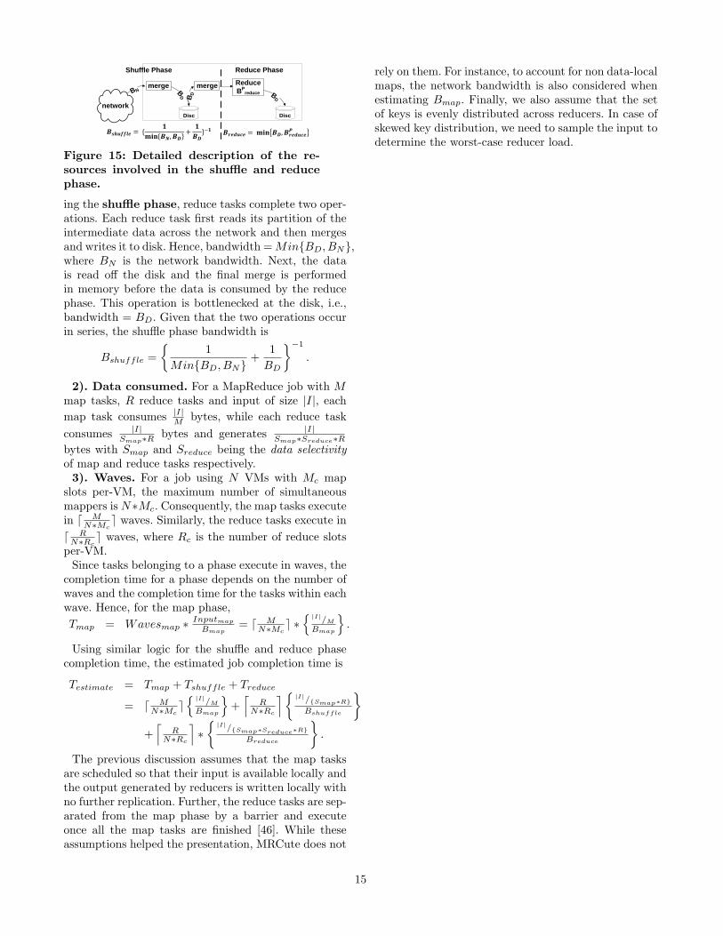
Figure 15: Detailed description of the re-sources involved in the shuffle and reducephase.

ing the shuffle phase, reduce tasks complete two oper-ations. Each reduce task first reads its partition of theintermediate data across the network and then mergesand writes it to disk. Hence, bandwidth =Min{BD, BN},where BN is the network bandwidth. Next, the datais read off the disk and the final merge is performedin memory before the data is consumed by the reducephase. This operation is bottlenecked at the disk, i.e.,bandwidth = BD. Given that the two operations occurin series, the shuffle phase bandwidth is

Bshuffle ={

1Min{BD, BN}

+1BD

}−1

.

2). Data consumed. For a MapReduce job with Mmap tasks, R reduce tasks and input of size |I|, eachmap task consumes |I|M bytes, while each reduce taskconsumes |I|

Smap∗R bytes and generates |I|Smap∗Sreduce∗R

bytes with Smap and Sreduce being the data selectivityof map and reduce tasks respectively.

3). Waves. For a job using N VMs with Mc mapslots per-VM, the maximum number of simultaneousmappers is N ∗Mc. Consequently, the map tasks executein d M

N∗Mce waves. Similarly, the reduce tasks execute in

d RN∗Rc

e waves, where Rc is the number of reduce slotsper-VM.

Since tasks belonging to a phase execute in waves, thecompletion time for a phase depends on the number ofwaves and the completion time for the tasks within eachwave. Hence, for the map phase,Tmap = Wavesmap ∗ Inputmap

Bmap= d M

N∗Mce ∗{ |I|/M

Bmap

}.

Using similar logic for the shuffle and reduce phasecompletion time, the estimated job completion time is

Testimate = Tmap + Tshuffle + Treduce

= d MN∗Mc

e{ |I|/M

Bmap

}+⌈

RN∗Rc

⌉{ |I|/{Smap∗R}Bshuffle

}+⌈

RN∗Rc

⌉∗{|I|/{Smap∗Sreduce∗R}

Breduce

}.

The previous discussion assumes that the map tasksare scheduled so that their input is available locally andthe output generated by reducers is written locally withno further replication. Further, the reduce tasks are sep-arated from the map phase by a barrier and executeonce all the map tasks are finished [46]. While theseassumptions helped the presentation, MRCute does not

rely on them. For instance, to account for non data-localmaps, the network bandwidth is also considered whenestimating Bmap. Finally, we also assume that the setof keys is evenly distributed across reducers. In case ofskewed key distribution, we need to sample the input todetermine the worst-case reducer load.

15